Classical Stückelberg interferometry of a nanomechanical two-mode system

Abstract

The transition from classical to quantum mechanics has intrigued scientists in the past and remains one of the most fundamental conceptual challenges in state-of-the-art physics. Beyond the quantum mechanical correspondence principle, quantum-classical analogies have attracted considerable interest. In this work, we present classical two-mode interference for a nanomechanical two-mode system, realizing classical Stückelberg interferometry. In the past, Stückelberg interferometry has been investigated exclusively in quantum mechanical two-level systems. Here, we experimentally demonstrate a classical analog of Stückelberg interferometry taking advantage of coherent energy exchange between two-strongly coupled, high quality factor nanomechanical resonator modes. Furthermore, we provide an exact theoretical solution for the double passage Stückelberg problem which reveals the analogy of the return probabilities in the quantum mechanical and the classical version of the problem. This result qualifies classical two-mode systems at large as a testbed for quantum mechanical interferometry.

I Introduction

In 1932, Stückelberg Stückelberg (1932) investigated the dynamics of a quantum two-level system undergoing a double passage through an avoided crossing. For a given energy splitting, an interference pattern arises that depends on the transit time and the rate at which the energy of the system is changed. This discovery lead to the advent of Stückelberg interferometry that allows for characterizing the parameters of a two-level system or for achieving quantum control over the system Shevchenko et al. (2010). Stückelberg interferometry has been intensively studied in a variety of quantum systems, e.g., Rydberg atoms Yoakum et al. (1992), ultracold atoms and molecules Mark et al. (2007), dopants Dupont-Ferrier et al. (2013), nanomagnets Wernsdorfer et al. (2000), quantum dots Petta et al. (2010); Gaudreau et al. (2012); Ribeiro et al. (2013); Forster et al. (2014) and superconducting qubits Oliver et al. (2005); Sillanpää et al. (2006); Lahaye et al. (2009); Shevchenko et al. (2012); Gong et al. (2016) as well as theoretically in a semi-classical optomechanical approach Heinrich et al. (2010). Here, we experimentally study a classical analog of Stückelberg interferometry, the coherent energy exchange of two strongly coupled classical high Q nanomechanical resonator modes, which can be seen as two high occupancy phonon states. We employ the analytical solution Vitanov and Garraway (1996) of the Landau-Zener problem describing the single passage through the avoided crossing Landau (1932); Zener (1932); Stückelberg (1932); Majorana (1932) to analyze the Stückelberg problem, demonstrating that the classical coherent exchange of energy follows the same dynamics as the coherent tunnelling of a quantum mechanical two-level system.
The past years have seen the advent of highly versatile nanomechanical systems based on strongly coupled, high quality factor modes Okamoto et al. (2013); Faust et al. (2013); Shkarin et al. (2014). The strong coupling generates a pronounced avoided crossing of the classical mechanical modes realizing a nanomechanical two-mode system that can be employed as a testbed for the dynamics at energy level crossings Okamoto et al. (2013); Faust et al. (2013); Shkarin et al. (2014); Faust et al. (2012a).
In the case of a quantum two-level system, e.g. a spin-1/2, a single passage through the avoided crossing results in Landau-Zener dynamics originating from the tunnelling of a quantum mechanical excitation between two quantum states Landau (1932). In the classical case, the exchange of excitation energy between two strongly coupled mechanical modes represents a well established analogy to this process Maris and Xiong (1988); Shore et al. (2009). From a quantum mechanical point of view, the two classical modes can be described as high occupancy states with billions of phonons residing in the respective resonator mode, where the discrete bosonic energy levels are thermally smeared out orders of magnitude larger than their level spacing.
During a double passage through the avoided crossing within the coherence time of the system, phase is accumulated, leading to self-interference. This interference results in oscillations of the return probability, in a quantum mechanical context well-known as Stückelberg oscillations Stückelberg (1932), which have previously been studied in many quantum systems Petta et al. (2010); Gaudreau et al. (2012); Ribeiro et al. (2013); Gong et al. (2016); Sun et al. (2011). In the classical case, the return probability is analogous to the probability that the excitation, namely oscillation energy, coherently returns to the same mechanical mode. We experimentally demonstrate that phenomenon and present an exact theoretical solution of the classical Stückelberg problem, which demonstrates that the classical flow in the coherent classical system follows the same dynamics as the unitary evolution operator of a quantum mechanical two-level system. In this way, classical Stückelberg interferometry opens up a path to further investigate the transition from quantum to classical systems as has recently been demonstrated in the framework of ultracold atom experiments Lohse et al. (2016); Kaufman et al. (2016); Neuzner et al. (2016).

II Nanomechanical two-mode system

We experimentally explore a purely classical, mechanical two-mode system, consisting of two orthogonally polarized fundamental flexural modes of a nanomechanical resonator (Fig. 1 (a)). The flexural modes belong to the in-plane and out-of-plane vibration of a 50 µm long, 270 nm wide and 100 nm thick doubly clamped, high-stress silicon nitride (SiN) string resonator. Dielectric drive and control via electric gradient fields Rieger et al. (2012) as well as the microwave cavity enhanced, heterodyne dielectric detection scheme Faust et al. (2012b); Rieger et al. (2012); Faust et al. (2013) is provided via two adjacent gold electrodes as detailed in appendix A. Applying a dc voltage to the electrodes induces an electric polarization in the silicon nitride string, which, in turn, couples to the electric field gradient resulting in a quadratic resonance frequency shift with the applied voltage Rieger et al. (2012). The electric field gradients along the in- and out-of-plane direction have opposing signs, and hence an inverse tuning behavior. Whereas the out-of-plane oscillation shifts to higher mechanical resonant frequencies, the in-plane oscillation decreases in frequency with the applied dc voltage Rieger et al. (2012). Hence, the inherent frequency offset of in-plane and out-of-plane oscillation, induced by the rectangular cross-section of the string, can be compensated. Furthermore, the applied inhomogeneous electric field induces a strong coupling between the two modes Faust et al. (2012a). Near resonance, they hybridize into normal modes Faust et al. (2013), diagonally polarized along $\pm 45$°. A pronounced avoided crossing with level splitting $\Delta/2\pi$ reflects the strong mutual coupling of the flexural mechanical modes as depicted in Fig. 1 (b). In order to study Stückelberg interferometry, we perform a double passage through the avoided crossing using a fast triangular voltage ramp. We initialize the system at voltage $U_{i}$ in the lower branch of the avoided crossing via a resonant sinusoidal drive tone at the resonance frequency $\omega_{\mathrm{1}}(U_{\mathrm{i}})/2\pi$ of the out-of-plane oscillation (cf. Fig. 1 (b)). As illustrated in Fig. 1 (c), at time $t=0$, a fast triangular voltage ramp with voltage sweep rate $\beta$ up to the peak voltage $U_{\mathrm{p}}$, and back to the read-out voltage $U_{\mathrm{f}}$ is applied to tune the system through the avoided crossing. Note that the ramp detunes the system from the resonant drive and the mechanical energy starts to decay exponentially. At $U_{\mathrm{f}}$, we measure the exponential decay of the mechanical oscillation in the lower branch after time $t=\vartheta+\varepsilon$, where $\vartheta$ is the duration of the ramp, i.e. the propagation time, and $\varepsilon$ serves as temporal offset to avoid transient effects. The signal is extrapolated and evaluated at time $\vartheta$ by an exponential fit and normalized to the signal intensity at the initialization point ($t=0$), consequently yielding a normalized squared return amplitude. The return signal has to be measured at the read-out voltage $U_{\mathrm{f}}$ at $\omega_{1}(U_{\mathrm{f}})/2\pi$ since the fixed rf drive tone at $\omega_{1}(U_{\mathrm{i}})/2\pi$ cannot be turned off during the measurement. The presented voltage sequence is analogous to the one employed in Ref. Sun et al. (2011) and differs from the frequently performed periodic driving scheme in Stückelberg interferometry experiments Shevchenko et al. (2010).

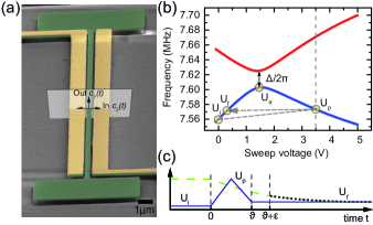
Figure 1: Nanomechanical resonator and measurement scheme. (a) False color scanning electron micrograph of the 50 µm long, 270 nm wide and 100 nm thick silicon nitride string (green) flanked by two adjacent gold electrodes in oblique view. Arrows indicate the flexural mode polarizations out-of-plane (Out) and in-plane (In). The normalized amplitude of the respective mode is denoted $c_{1}(t)$ for out-of-plane polarization and $c_{2}(t)$ for in-plane polarization as explained in the text. (b) Avoided mode crossing of sample A exhibiting a frequency splitting of $\Delta/2\pi=22.614$ kHz at the avoided crossing voltage $U_{\mathrm{a}}=U_{\mathrm{i}}+1.471$ V$=9.371$ V. The lower (out-of-plane) mode is excited at frequency $\omega_{\mathrm{1}}(U_{\mathrm{i}})/2\pi=7.560$ MHz defined by the initialization voltage $U_{\mathrm{i}}$. An additional sweep voltage applies a triangular voltage ramp rising to a maximum of $U_{\mathrm{p}}$ and back to the read-out voltage $U_{\mathrm{f}}=U_{\mathrm{i}}+0.2$ V$=8.1$ V, thus transgressing the avoided crossing twice. The sweep voltage also decouples the mode from the fixed-frequency drive, consequently inducing an exponential decay of the amplitude. (c) Time evolution of the sweep voltage beginning at $t=0$, increasing to $U_{\mathrm{p}}$ and returning to $U_{\mathrm{f}}$ after interval $\vartheta$. The mechanical signal power (green dashed line) is measured after a delay $\varepsilon$ and a fit (black dotted line) is used to extract its magnitude at time $t=\vartheta$. The measured return signal is normalized to the mechanical signal power at $t=0$.

III Finite time Stückelberg theory

We follow the work of Novotny Novotny (2010) to derive the classical flow (Hamiltonian flow Arnold (1989)) describing the dynamics of the system in the vicinity of the avoided crossing. We start with Newton’s equation of motion for the displacement

$$m\ddot{u}_{1}(t) =-k_{1}u_{1}(t)-\kappa\left[u_{1}(t)-u_{2}(t)\right],$$ (1)

$$m\ddot{u}_{2}(t) =-k_{2}u_{2}(t)+\kappa\left[u_{1}(t)-u_{2}(t)\right],$$

with $u_{j}(t)$ ($j=1,2$) describing, respectively, the out-of-plane ($j=1$) and in-plane ($j=2$) displacement of the center of mass of the oscillator, $k_{j}$ is the spring constant of mode $j$, $\kappa$ the coupling constant between the two modes and $m$ is the effective mass of the oscillator. We look for solutions of the form $u_{j}(t)=c_{j}(t)\exp[i\omega_{1}t]$ with $c_{j}(t)$ a normalized amplitude, i.e. $\left|c_{1}(t)\right|^{2}+\left|c_{2}(t)\right|^{2}=1$. In the experimentally relevant limit where $\kappa/k_{1}\ll 1$, the amplitudes $c_{j}(t)$ are slowly varying in time as compared to the oscillatory function $\exp[i\omega_{1}t]$. As a consequence, it is possible to neglect the second derivates $\ddot{c}_{j}(t)$ in the equations describing the motion of $c_{j}(t)$, which are obtained by replacing the ansatz for $u_{j}(t)$ in Eq. (1). Thus, the system of coupled differential equations describing the evolution of the normalized amplitudes is

$$\begin{cases}i\dot{c}_{1}=\frac{\kappa}{2\omega_{1}m}c_{2},\\ i\dot{c}_{2}=\frac{\kappa}{2\omega_{1}m}c_{1}-\frac{(\omega_{2}-\omega_{1})^{2}}{2\omega_{1}}c_{2},\end{cases}$$ (2)

with $\omega_{\mathrm{j}}=\sqrt{k_{j}/m}$ the bare resonance frequency of mode $j$ in units of $2\pi$. In the vicinity of the avoided crossing, where the modes can exchange energy, we have $\omega_{2}\simeq\omega_{1}$ such that $(\omega_{2}-\omega_{1})^{2}/2\omega_{1}\simeq\omega_{2}-\omega_{1}$. If we further assume $\omega_{2}-\omega_{1}\simeq\alpha t$, with $\alpha$ the frequency sweep rate, and define $\Delta=\left|\lambda\right|=\kappa/(m\omega_{1})$, Eq. (2) reduces to

$$i\dot{\mathbf{c}}(t)=H(t)\mathbf{c}(t),$$ (3)

with $\mathbf{c}(t)=(c_{1}(t)\,c_{2}(t))^{\mathrm{T}}$ and

$$H(t)=\begin{pmatrix}0&&\frac{\lambda}{2}\\ \frac{\lambda}{2}&&-\alpha t\end{pmatrix}.$$ (4)

Since we are interested in multiple passages through the avoided crossing, we look for the classical flow $\varphi(t,t_{\mathrm{i}})$ defining the state of the system at time $t$ given that we know its state at some prior time $t_{\mathrm{i}}$, $\mathbf{c}(t)=\varphi(t,t_{\mathrm{i}})\mathbf{c}(t_{\mathrm{i}})$. Typically, $\mathbf{c}(t_{\mathrm{i}})$ is the initial condition of the system. One can show that the classical flow obeys the same differential equation as $\mathbf{c}(t)$, $i\dot{\varphi}(t,t_{\mathrm{i}})=H(t)\varphi(t,t_{\mathrm{i}})$. By applying the time-dependent unitary transformation $S(t)=\exp[i\alpha t^{2}/4]\mathbbm{1}_{2}$ to the classical flow, i.e. $\varphi(t,t_{\mathrm{i}})=S(t)\tilde{\varphi}(t,t_{\mathrm{i}})S^{\dagger}(t_{\mathrm{i}})$, we find that $\tilde{\varphi}(t,t_{\mathrm{i}})$ obeys the differential equation,

$$i\dot{\tilde{\varphi}}(t,t_{\mathrm{i}}) =\left(S^{\dagger}(t)H(t)S(t)-iS^{\dagger}(t)\dot{S}(t)\right)\tilde{\varphi}(t,t_{\mathrm{i}})$$ (5)

$$=\tilde{H}(t)\tilde{\varphi}(t,t_{\mathrm{i}}),$$

with

$$\tilde{H}(t)=\begin{pmatrix}\frac{\alpha t}{2}&&\frac{\lambda}{2}\\ \frac{\lambda}{2}&&-\frac{\alpha t}{2}\end{pmatrix},$$ (6)

where $\mathbbm{1}_{2}$ denotes the unity operator in two dimensions. Equation (5) coincides with the Schrödinger equation for the unitary evolution operator of the Landau-Zener problem with $\hbar$ set to 1, for which an exact finite-time solution is known Vitanov and Garraway (1996) (see also appendix B). With the help of the classical flow, one can easily calculate the state of the system after a double passage through the avoided crossing (Stückelberg problem). We find

$$\mathbf{c}(t)=\varphi_{\mathrm{b}}(t,-t_{\mathrm{p}})\varphi(t_{\mathrm{p}},t_{\mathrm{i}})\mathbf{c}(t_{\mathrm{i}}),$$ (7)

with $\varphi_{\mathrm{b}}(t,t_{\mathrm{i}})=\sigma_{x}\varphi(t,t_{\mathrm{i}})\sigma_{x}$ describing the evolution of the system during the back sweep (see appendix B) where $\sigma_{x}$ denotes the Pauli matrix in x-direction and $t_{\mathrm{p}}$ labels the time at which the forward (backward) sweep stops (starts). From Eq. (7), one can obtain the return probability to mode 1,

$$P_{1\to 1}=$$ (8)

$$\left|\varphi_{11}(t_{\mathrm{p}},t_{\mathrm{i}})\varphi_{11}^{\ast}(t,-t_{\mathrm{p}})+\varphi_{12}^{\ast}(t_{\mathrm{p}},t_{\mathrm{i}})\varphi_{12}^{\ast}(t,-t_{\mathrm{p}})\right|^{2},$$

with $\varphi_{ij}(t,t_{\mathrm{i}})$ the matrix elements of $\varphi(t,t_{\mathrm{i}})$. Note that we use the frequency sweep rate $\alpha$ in the theory, which is converted to the experimentally accessible voltage sweep rate $\beta$ via a conversion factor $\zeta=55.042$ kHz/V as elucidated in appendix C.
The analogy between the unitary evolution operator and the classical flow, both expressed in the basis of uncoupled states (modes), allows one to draw the analogy to the quantum mechanical return probability in Stückelberg interferometry. In principle, this corresponds to the averaging over all possible Fock states in the phonon distribution of the mechanical resonator mode. The normalized amplitudes are associated with the normalized energy in each resonator mode and differ conceptually from the probability that a quantum mechanical two-level system is found in either of the two quantum states. Nevertheless, the dynamics of the normalized amplitudes in classical Stückelberg interferometry is analogous to the dynamics of the quantum mechanical probabilities in the sense that the coherent exchange of oscillation energy between two coupled modes can be associated with the transfer of population between two quantum states. A more detailed discussion and comparison of our theoretical approach to previous models  Maris and Xiong (1988); Vitanov and Garraway (1996); Shore et al. (2009); Shevchenko et al. (2010) will be published elsewhere Seitner et al. (2016).
Note that Stückelberg interferometry does in the contrary not apply to the case of two coupled quantum harmonic oscillators in a general quantum state. In that case, the effective model describing the dynamics would resemble that of the multiple-crossings Landau-Zener problem Usuki (1997), which leads to a much more complex dynamics than the standard Stückelberg dynamics. Only in the case of a singly populated quantum level, i.e., the single phonon Fock state, and if the Hamiltonian of the system conserves the number of excitations, the discussed result is recovered.

IV Classical Stückelberg interferometry

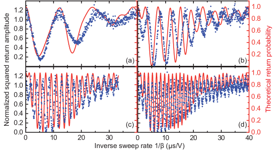
Figure 2: Classical Stückelberg oscillations. Normalized squared return amplitude (left axis, blue dots) and theoretically calculated return probability (right axis, red line) versus inverse sweep rate for fixed peak voltages of $U_{\mathrm{p}}=2.5$ V (a), $U_{\mathrm{p}}=3.5$ V (b), $U_{\mathrm{p}}=4.5$ V (c) and $U_{\mathrm{p}}=5.0$ V (d) measured on sample A.

Experimentally, we investigate classical Stückelberg oscillations with two different samples in a vacuum of $\leq$ $10^{-4}$ mbar. Sample A is investigated at 10 K in a temperature-stabilized pulse tube cryostat which offers a greatly enhanced stability of the electromechanical system against temperature fluctuations. Sample B is explored at room temperature in order to confirm the results and to check their stability under ambient temperature fluctuations. Note that in both experiments, the system operates deeply in the classical regime Faust et al. (2013) and does not exhibit any quantum mechanical properties. Sample A exhibits a mechanical quality factor $Q=\omega/\Gamma\approx 2\times 10^{5}$ and linewidth $\Gamma/2\pi\approx 40$ Hz at resonance frequency $\omega_{1}(U_{\mathrm{i}})/2\pi=7.560$ MHz of the 50 µm long string resonator ensuring classical coherence times in the millisecond regime Faust et al. (2013). The level splitting $\Delta/2\pi=22.614$ kHz exceeds the mechanical linewidth by almost three orders of magnitude, which puts the system deep into the strong coupling regime. We initialize the system at $U_{\mathrm{i}}=7.9$ V and apply triangular voltage ramps with different voltage sweep rates $\beta$ for a set of peak voltages $U_{\mathrm{p}}$. Figure 2 depicts the normalized squared return amplitude for different peak voltages and the theoretical return probabilities calculated without any free parameters. The normalized squared return amplitude may exceed a value of unity due to normalization artefacts which arise from the different signal magnitudes at the initialization and read-out voltages in addition to measurement errors. We observe clear oscillations in the return signal in good agreement with the theoretical predictions for lower peak voltages. As the number of oscillations increases for higher peak voltages, the deviation from the theoretical prediction is more pronounced. We attribute this to uncertainties and fluctuations of the characteristic sweep parameters of the system, which change under application of the voltage ramp and over time as discussed in appendices D and E. A further deviation arises from the assumption that a linear change of the voltage leads to a linear change of the difference in frequency. This is only an approximation since the mechanical resonance frequencies tune quadratically with the applied voltage Rieger et al. (2012). However, since most of the energy exchange happens in the vicinity of the avoided crossing, where the difference in frequency is linearized, one expects to see noticeable deviations from theory only for higher peak voltages.

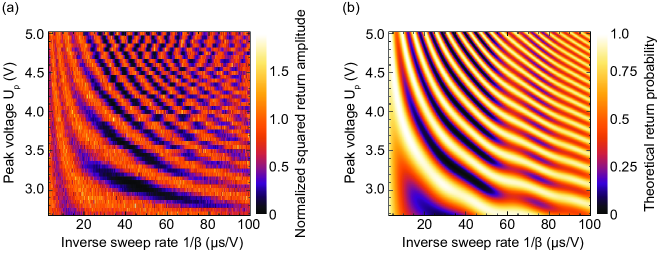
Figure 3: Comparison of experimental data and the theoretical model. (a) Color-coded normalized squared return amplitude versus inverse sweep rate and peak voltage measured on sample B. The dataset is not interpolated. (b) Color-coded theoretical return probability given by Eq. (9) versus inverse sweep rate and peak voltage for the equivalent data range. The theory is calculated with a single set of parameters, extracted from the avoided crossing illustrated in appendix C (Fig. C.1) and contains no free parameters.

In order to reproduce the experimental data and to test the stability of classical Stückelberg interferometry against fluctuations, we repeat the experiment on a second sample of the same design at room temperature (sample B, denoted by index ”B”). The now 55 µm long resonator has a mechanical linewidth of $\Gamma_{\mathrm{B}}/2\pi\approx 25$ Hz at frequency $\omega_{\mathrm{B,1}}(U_{\mathrm{B,i}})/2\pi=6.561$ MHz, which results in a quality factor of $Q_{\mathrm{B}}\approx 2.6\times 10^{5}$ at the initialization voltage $U_{\mathrm{B,i}}=10.4$ V and hence an improved mechanical lifetime of 6.21 ms. Furthermore, the sample exhibits a mode splitting of $\Delta_{\mathrm{B}}/2\pi=6.322$ kHz and a conversion factor of $\zeta_{\mathrm{B}}=19.224$ kHz/V. Figure 3 depicts a color-coded two-dimensional map of the normalized squared return amplitude as a function of the inverse voltage sweep rate $\beta$ and the peak voltage $U_{\mathrm{p}}$ alongside the theoretical return probability of the classical Stückelberg oscillations, again calculated with no free parameters. We investigate double passages up to a total propagation time of $\vartheta=1.0$ ms in the experiments conducted on sample B. To account for the decay of both modes when tuned away from the drive for the considerably longer ramps applied to sample B, we model the mechanical damping by an exponential decay with an averaged decay time $t_{0}=5.7\,\mathrm{ms}$. After a measurement time $t_{m}$, the probability to measure an excitation of mode $j$ is given by

$$\left|c_{j}(t_{m})\right|^{2}=\exp[-t_{m}/t_{0}]P_{1\to j},$$ (9)

with $P_{1\to 1}$ given by Eq. (8) and $P_{1\to 2}=1-P_{1\to 1}$. The experimental data shows remarkably good agreement with the theoretical predictions, despite temperature fluctuations of several kelvin per hour, which shift the mechanical resonance frequency up to 40 linewidths. In order to initialize the system at the same resonance frequency in each measurement, a feedback loop regulates the initialization voltage $U_{\mathrm{i}}$ (see appendix D). Consequently, the recording of a single horizontal scan at a fixed peak voltage in Fig. 3 (a) takes up to 16 hours, incorporating a non-negligible amount of fluctuations of the system parameters, such as e.g. the center voltage of the avoided crossing $U_{\mathrm{a}}$, which imposes considerable uncertainties on the parameters used for the theoretical calculations. To further illustrate the influence of fluctuations, Fig. 4 (a) and Fig. 4 (b) depict horizontal and vertical line-cuts of the two-dimensional map in Fig. 3 at $U_{\mathrm{p}}=3.3$ V and at inverse sweep rate $1/\beta=51.6$ µs/V, respectively. For small inverse sweep rates, i.e. very fast sweeps, the experimental data in Fig. 4 (a) deviates from the theoretical model due to a flattening of the voltage ramps in the room temperature experiment (see appendix E). For sweeps with $1/\beta\geq 50$ µs/V, the experimentally observed Stückelberg oscillations exhibit good agreement with the theoretical predictions even for the line-cut along the vertical peak voltage axis (cf. Fig. 4 (b)). Note that Fig. 4 depicts the best results from all datasets at room temperature. Further exemplary line-cuts are provided in appendix E, also exhibiting a clear oscillatory behavior in the normalized squared return amplitude, but incorporating larger deviations from theory in certain regions and therefore revealing fluctuations of system parameters over time, predominately induced by temperature drifts.

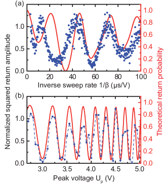
Figure 4: Exemplary classical Stückelberg oscillations of sample B. Line-cuts of Fig. 3 (a) and Fig. 3 (b). (a) Normalized squared return amplitude (left axis, blue dots) and theoretically calculated return probability given by Eq. (9) (right axis, red line) versus inverse sweep rate for a fixed peak voltage $U_{\mathrm{p}}=3.3$ V. (b) Same quantities as above but plotted as a function of peak voltage for a fixed inverse sweep rate $1/\beta=51.6$ µs/V. Blue dots are joined by blue dashed lines for illustration reasons.

V Conclusion and Outlook

In conclusion, we have demonstrated classical Stückelberg oscillations which have previously been experimentally observed exclusively in the framework of quantum mechanics Shevchenko et al. (2010); Petta et al. (2010); Gaudreau et al. (2012); Sun et al. (2011). Providing an exact solution for the Stückelberg problem Stückelberg (1932), we have established the analogy between the quantum mechanical and the classical return probability. In this way, we have demonstrated that the coherent exchange of energy between two strongly coupled classical nanomechanical resonator modes follows the same dynamics as the exchange of excitations in a quantum mechanical two-level system in the framework of Stückelberg interferometry. However, this analogy generally breaks down if the two coupled harmonic oscillators start to enter the quantum regime due to multilevel population transfer effects Usuki (1997). This aspect will allow for the future investigation of dissimilarities, homologies and analogies of classical and quantum mechanical systems as recently studied in ultracold atoms Lohse et al. (2016); Kaufman et al. (2016); Neuzner et al. (2016). Overall, we have found remarkably good agreement between experiment and theory. However, parameter regimes yielding larger deviations are reminiscent of the sensitivity of the exact Stückelberg solution to the initial system parameters, such as the position of the avoided crossing, and hence to fluctuations in the system. This circumstance, in turn, might be exploited for future investigations in resonator metrology of decoherence and noise, adapting the approach to employ Stückelberg interferometry to characterize the coherence of a qubit Forster et al. (2014). Furthermore, the possibility to create a superposition state of two mechanical modes may allow for future application as highly sensitive nanomechanical interferometers Xu et al. (2016); Rossi et al. (2016); Mercier de Lépinay et al. (2016) analogous to the applications with cold atom and molecule matter-wave interferometers Andrews et al. (1997); Castin and Dalibard (1997); Mark et al. (2007); Kohstall et al. (2011), whereas the presence and implications of, e.g., phase noise Maillet et al. (2015) can be resolved by a change in resonator population and interference pattern. Classical Stückelberg interferometry should not be limited to the presented strongly coupled, high quality factor nanomechanical string resonator modes Faust et al. (2013), but can in principle be observed in every classical two-mode system exhibiting the possibility of a double passage through an avoided crossing within the classical coherence time.

Appendix A The nanoelectromechanical system

The nanomechanical device and experimental set-up are depicted in Fig. A.1. The sample investigated at a temperature of 10 K (sample A) consists of a 50 µm long, 270 nm wide and 100 nm thick doubly clamped silicon nitride (SiN) string resonator. The room temperature measurements were conducted on a similar sample (sample B), differing only in its resonator length of 55 µm. As stated in the main text, the temperature does not affect the purely classical character of the system. The string resonators exhibit a high intrinsic tensile pre-stress of $\sigma_{\mathrm{SiN}}=1.46$ GPa resulting from the LPCVD deposition of the SiN film on the fused silica substrate. This high stress translates into large intrinsic mechanical quality factors of up to $Q\approx 500,000$, which reduce quadratically with the applied dc tuning voltage in the experiment as a result of dielectric damping Rieger et al. (2012). Dielectric drive, detection and control are provided via two adjacent gold electrodes in an all integrated microwave cavity enhanced transduction scheme Faust et al. (2012b, a); Rieger et al. (2012); Faust et al. (2013).

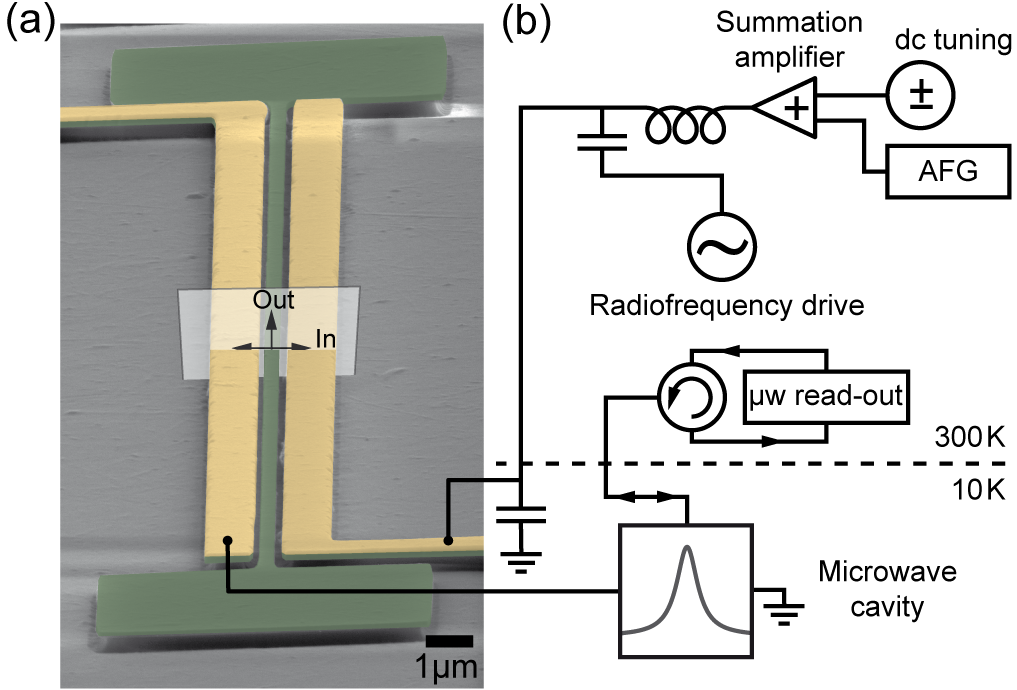
Figure A.1: Nanoelectromechanical system. (a) False color scanning electron micrograph of the 50 µm long, 270 nm wide and 100 nm thick silicon nitride string (green) in oblique view. The adjacent 1 µm wide gold electrodes (yellow) are processed on top of the silicon nitride layer. Arrows indicate the flexural mode polarizations out-of-plane (Out) and in-plane (In). (b) Electrical transduction set-up. The arbitrary function generator (AFG) ramp voltage and the dc tuning voltage are added via a summation amplifier and then combined with the rf drive using a bias tee. The microwave read-out is bypassed by the second capacitor, acting as ground path for the microwave cavity.

In the experiment, we consider the two orthogonally polarized fundamental flexural modes of the nanomechanical string resonator, namely the oscillation perpendicular to the sample plane (out-of-plane) and the oscillation parallel to the sample plane (in-plane). Applying a dc voltage to one of the two gold electrodes induces an electric polarization in the silicon nitride string resonator, which couples to the field gradient of the inhomogeneous electric field. Consequently, the mechanical resonance frequencies tune quadratically with the applied dc voltage as depicted in Fig. A.2. Whereas the out-of-plane resonance (Out) tunes towards higher resonance frequencies as a function of dc voltage, the resonance frequency of the in-plane mode (In) decreases Rieger et al. (2012). Dielectrical tuning of both modes into resonance reveals a pronounced avoided crossing originating from the strong mutual coupling induced by the inhomogeneous electric field. In the coupling region, the mechanical modes hybridize into diagonally ($\pm$45°) polarized eigenmodes of the strongly coupled system.

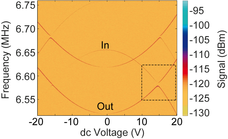
Figure A.2: Dielectric frequency tuning. Color-coded frequency spectrum of sample B as a function of applied dc tuning voltage. The resonance frequency of the 55 µm long resonator’s fundamental out-of-plane oscillation (Out) increases quadratically as a function of dc voltage. The resonance frequency of the corresponding in-plane mode (In) decreases quadratically. Tuning both modes into resonance, they exhibit a pronounced avoided crossing indicated by the black dashed rectangle. This particular region is displayed in Fig. C.1 (a). The additional resonances in the spectrum originate from a different mechanical resonator which is coupled to the same microwave cavity.

Appendix B Theoretical Model

In this section, we derive an exact expression for the classical return probability. A detailed discussion and comparison of our theoretical approach to previous models will be published elsewhere Seitner et al. (2016).
We start by solving the system of first-order differential equations defined in Eq. (5) of the main text. Since these equations are formally identical to the Schrödinger equation for the (quantum) Landau-Zener problem, we can follow the work of Vitanov et al.  Vitanov and Garraway (1996) to derive the classical flow, $\mathbf{\tilde{c}}(\tau)=\tilde{\varphi}(\tau,\tau_{\mathrm{i}})\mathbf{\tilde{c}}(\tau_{\mathrm{i}})$ with $\mathbf{\tilde{c}}(\tau)=(\tilde{c}_{1}(\tau)\,\,\tilde{c}_{2}(\tau))^{\mathrm{T}}$. Here, $\tau=\sqrt{\alpha}t$ is a dimensionless time and $\tau_{\mathrm{i}}$ the initial dimensionless time. Note that we use dimensionless times in this chapter in order to provide a derivation which is consistent with the work of Vitanov et al.  Vitanov and Garraway (1996). The equations in dependence of times in the main text can be recovered by replacement of the dimensionless times following the above definition. In appendix C, we provide the explicit conversion from experimentally accessible parameters to the dimensionless times. We find

$$\begin{pmatrix}\tilde{c}_{1}(\tau)\\ \tilde{c}_{2}(\tau)\end{pmatrix}=\begin{pmatrix}\tilde{\varphi}_{11}(\tau,\tau_{\mathrm{i}})&&\tilde{\varphi}_{12}(\tau,\tau_{\mathrm{i}})\\ -\tilde{\varphi}_{12}^{\ast}(\tau,\tau_{\mathrm{i}})&&\tilde{\varphi}_{11}^{\ast}(\tau,\tau_{\mathrm{i}})\end{pmatrix}\begin{pmatrix}\tilde{c}_{1}(\tau_{\mathrm{i}})\\ \tilde{c}_{2}(\tau_{\mathrm{i}}),\end{pmatrix}$$ (10)

with

$$\tilde{\varphi}_{11}(\tau,\tau_{\mathrm{i}})=$$ (11)

$$\frac{\Gamma\left(1+i\frac{\eta^{2}}{4}\right)}{\sqrt{2\pi}}\left[D_{-1-i\frac{\eta^{2}}{4}}\left(\mathrm{e}^{-i\frac{3\pi}{4}}\tau_{\mathrm{i}}\right)D_{-i\frac{\eta^{2}}{4}}\left(\mathrm{e}^{i\frac{\pi}{4}}\tau\right)\right.$$

$$\phantom{=}+\left.D_{-1-i\frac{\eta^{2}}{4}}\left(\mathrm{e}^{i\frac{\pi}{4}}\tau_{\mathrm{i}}\right)D_{-i\frac{\eta^{2}}{4}}\left(\mathrm{e}^{-i\frac{3\pi}{4}}\tau\right)\right],$$

and

$$\tilde{\varphi}_{12}(\tau,\tau_{\mathrm{i}})=$$ (12)

$$\frac{\Gamma\left(1+i\frac{\eta^{2}}{4}\right)}{\sqrt{2\pi}}\frac{2}{\eta}\mathrm{e}^{-i\frac{\pi}{4}}\left[D_{-i\frac{\eta^{2}}{4}}\left(\mathrm{e}^{-i\frac{3\pi}{4}}\tau_{\mathrm{i}}\right)D_{-i\frac{\eta^{2}}{4}}\left(\mathrm{e}^{i\frac{\pi}{4}}\tau\right)\right.$$

$$\phantom{=}-\left.D_{-i\frac{\eta^{2}}{4}}\left(\mathrm{e}^{i\frac{\pi}{4}}\tau_{\mathrm{i}}\right)D_{-i\frac{\eta^{2}}{4}}\left(\mathrm{e}^{-i\frac{3\pi}{4}}\tau\right)\right].$$

Here, $\eta=\lambda/\sqrt{\alpha}$ is the dimensionless coupling, $\Gamma(z)$ is the Gamma function, and $D_{\nu}(z)$ is the parabolic cylinder function. To find the flow describing the evolution of the amplitudes defined in Eq. (2), we apply the unitary transformation defined in the main text, $\varphi(\tau,\tau_{\mathrm{i}})=S(\tau)\tilde{\varphi}(\tau,\tau_{\mathrm{i}})S^{\dagger}(\tau_{\mathrm{i}})$, with

$$S(\tau)=\exp\left[\frac{i}{4}\tau^{2}\right]\mathbbm{1}_{2}.$$ (13)

We find

$$\varphi(\tau,\tau_{\mathrm{i}})=\exp\left[\frac{i}{4}(\tau^{2}-\tau_{\mathrm{i}}^{2})\right]\tilde{\varphi}(\tau,\tau_{\mathrm{i}}).$$ (14)

The flow $\varphi(\tau,\tau_{\mathrm{i}})$ describes the evolution of the normalized amplitudes for a forward sweep; the frequency of mode $1$ ($2$) increases (decreases) with time. This implies that the back sweep cannot be described by $\varphi(\tau,\tau_{\mathrm{i}})$ since during the evolution the frequency of mode $1$ ($2$) decreases (increases). Hence, the system of coupled differential equations describing the dynamics during the backward sweep (denoted by index ”b”) is given by

$$i\begin{pmatrix}\dot{\tilde{c}}_{\mathrm{1,b}}\\ \dot{\tilde{c}}_{\mathrm{2,b}}\end{pmatrix}=\begin{pmatrix}-\frac{\alpha t}{2}&&\frac{\lambda}{2}\\ \frac{\lambda}{2}&&\frac{\alpha t}{2}\end{pmatrix}\begin{pmatrix}\tilde{c}_{\mathrm{1,b}}\\ \tilde{c}_{\mathrm{2,b}}\end{pmatrix}.$$ (15)

The solutions of Eq. (15) can be obtained analogously to the forward flow since the matrices appearing in Eq. (6) of the main text and Eq. (15) are related by a unitary transformation. We find

$$\tilde{\varphi}_{\mathrm{b}}(\tau,\tau_{\mathrm{i}}) =\sigma_{x}\tilde{\varphi}(\tau,\tau_{\mathrm{i}})\sigma_{x}$$ (16)

$$=\begin{pmatrix}\tilde{\varphi}_{11}^{\ast}(\tau,\tau_{\mathrm{i}})&&-\tilde{\varphi}_{12}^{\ast}(\tau,\tau_{\mathrm{i}})\\ \tilde{\varphi}_{12}(\tau,\tau_{\mathrm{i}})&&\tilde{\varphi}_{11}(\tau,\tau_{\mathrm{i}})\end{pmatrix},$$

where $\sigma_{x}$ denotes the Pauli matrix in the $x$-direction. The flow describing the evolution of the amplitudes $c_{1}(t)$ and $c_{2}(t)$ during the back sweep is obtained as previously, we have

$$\varphi_{\mathrm{b}}(\tau,\tau_{\mathrm{i}})=\exp\left[\frac{i}{4}(\tau^{2}-\tau_{\mathrm{i}}^{2})\right]\tilde{\varphi}_{\mathrm{b}}(\tau,\tau_{\mathrm{i}}).$$ (17)

The state of the system after a double sweep is given by

$$\mathbf{c}(\tau)=\varphi_{\mathrm{b}}(\tau,-\tau_{\mathrm{p}})\varphi(\tau_{\mathrm{p}},\tau_{\mathrm{i}})\mathbf{c}(\tau_{\mathrm{i}}),$$ (18)

where $\tau_{\mathrm{p}}$ labels the time at which the first sweep stops and $-\tau_{\mathrm{p}}$ corresponds to the initial time of the back sweep (cf. Eq. (7) of the main text). As stated in Eq. (8) of the main text, the probability to return to mode $1$ is then given by

$$P_{1\to 1}(\tau,\tau_{\mathrm{p}},\tau_{\mathrm{i}})=$$ (19)

$$\left|\varphi_{11}(\tau_{\mathrm{p}},\tau_{\mathrm{i}})\varphi_{11}^{\ast}(\tau,-\tau_{\mathrm{p}})+\varphi_{12}^{\ast}(\tau_{\mathrm{p}},\tau_{\mathrm{i}})\varphi_{12}^{\ast}(\tau,-\tau_{\mathrm{p}})\right|^{2}.$$

Appendix C Conversion factor calibration

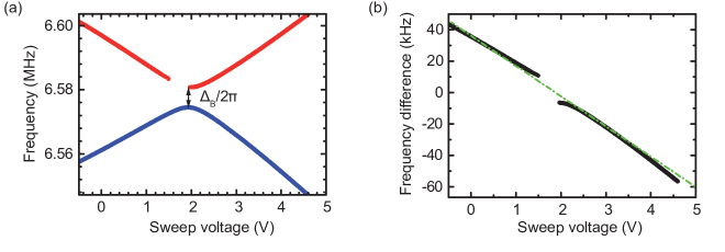
Figure C.1: Calibration of the conversion factor. (a) Avoided crossing region of sample B. A sweep voltage equal to zero corresponds to the initialization point $U_{\mathrm{i}}=10.4$ V. The two modes exhibit a frequency splitting of $\Delta_{\mathrm{B}}/2\pi=6.322$ kHz at the avoided crossing voltage $U_{\mathrm{a}}=U_{\mathrm{i}}+1.958$ V$=12.358$ V. The gap in the upper branch (red) results from a signal detection efficiency of the particular mode polarization below the noise level. (b) Frequency difference of the two modes (black) and averaged slope of the linearized frequency tuning illustrated by green dash-dotted line.

In the theoretical model, the state of the system after a double passage through the avoided crossing depends on characteristic sweep times. Experimentally, we realize this double passage by the application of fast triangular voltage ramps, tuning the resonant frequency of the mechanical modes Rieger et al. (2012). In the following, we focus on sample B to illustrate how the different times are obtained.
We initialize the resonance in the lower frequency branch at the voltage $U_{\mathrm{i}}=10.4$ V, where we apply a continuous sinusoidal drive tone at $\omega_{\mathrm{1}}(U_{\mathrm{i}})/2\pi=6.561$ MHz. We then ramp the sweep voltage up to the peak voltage $U_{\mathrm{p}}$ across the avoided crossing at voltage $U_{\mathrm{a}}=U_{\mathrm{i}}+1.958$ V$=12.358$ V and then back to the read-out voltage $U_{\mathrm{f}}=U_{\mathrm{i}}+0.5$ V$=10.9$ V, where the oscillation energy is read-out again in the lower frequency branch. The offset of the read-out voltage with respect to the initialization voltage is necessary since we cannot stop the sinusoidal drive tone at $\omega_{\mathrm{1}}(U_{\mathrm{i}})/2\pi$ during the experiment. For a fixed peak voltage $U_{\mathrm{p}}$ the voltage sweep is performed for different voltage sweep rates $\beta$, given in the experimental units $[\beta]=\,$V/s. In the theoretical model, the frequency difference of the two modes in units of 2$\pi$ is approximated by $\omega_{2}-\omega_{1}\simeq\alpha t$, where the sweep rate $\alpha$ has the dimensions $[\alpha]=2\pi\times$ Hz/s. Consequently, we introduce the conversion factor $\zeta$ from voltage to frequency, defined via the relation

$$\alpha=2\pi\times\zeta\beta.$$ (20)

Figure C.1 illustrates the calibration of the conversion factor. As conventional in experiments on Stückelberg interferometry, the frequency difference of the two mechanical modes is approximated to be linear in time, i.e. linear in sweep voltage. In our particular system the resonance frequencies of the mechanical flexural modes tune quadratically with voltage outside of the avoided crossing (see Fig. A.2). Nevertheless, for the designated region around the avoided crossing, the two frequency branches can be linearized as follows. We take the frequency difference of both modes before and after the avoided crossing (cf. Fig. C.1 (b)), respectively, and extract the slopes via a linear fit. The two different slopes on the left and the right hand side of the avoided crossing are averaged, yielding an effective conversion factor (dash-dotted green line)

$$\zeta=19.224\,\mathrm{\frac{kHz}{V}}.$$ (21)

Depending on the specific peak voltage $U_{\mathrm{p}}$, one could take into account a weighted average of the two slopes in order to mitigate the deviation of the quadratic frequency tuning from the linear approximation. Here, one has to point out deliberately that we neglect any weighted average, but take solely the above conversion factor for the calculation of the theoretical return probabilities. We are well aware of the fact that this linearization translates into a direct discrepancy between the theoretical model and the experimental results. Nevertheless, in our opinion, these discrepancies are prevailed by the benefits of a closed theoretical calculation using a single set of parameters which is supported by the remarkably good agreement between experiment and theory. Hence, we express the characteristic sweep times in the theoretical model by the following parameters extracted from the avoided crossing in Fig. C.1 (a):

$$\begin{aligned} &t_{\mathrm{i}}=-\frac{1}{\beta}(U_{\mathrm{a}}-U_{\mathrm{i}})=\frac{\tau_{\mathrm{i}}}{\sqrt{\alpha}}\\ &t_{\mathrm{p}}=\frac{1}{\beta}(\widetilde{U}_{\mathrm{p}}-U_{\mathrm{a}})=\frac{\tau_{\mathrm{p}}}{\sqrt{\alpha}}\\ &t_{\mathrm{f}}=\frac{1}{\beta}(U_{\mathrm{a}}-U_{\mathrm{f}})=\frac{\tau_{\mathrm{f}}}{\sqrt{\alpha}},\end{aligned}$$ (22)

where $\widetilde{U}_{\mathrm{p}}=U_{\mathrm{i}}+U_{\mathrm{p}}$. As explained above, the return probability is measured at the read-out voltage $U_{\mathrm{f}}\neq U_{\mathrm{i}}$. Consequently, we replace $\tau$ by $\tau_{\mathrm{f}}$ in the back sweep of the theory, which modifies Eq. (19) to

$$P_{1\to 1}(\tau_{\mathrm{f}},\tau_{\mathrm{p}},\tau_{\mathrm{i}})=$$ (23)

$$\left|\varphi_{11}(\tau_{\mathrm{p}},\tau_{\mathrm{i}})\varphi_{11}^{\ast}(\tau_{\mathrm{f}},-\tau_{\mathrm{p}})+\varphi_{12}^{\ast}(\tau_{\mathrm{p}},\tau_{\mathrm{i}})\varphi_{12}^{\ast}(\tau_{\mathrm{f}},-\tau_{\mathrm{p}})\right|^{2}.$$

Appendix D Temperature fluctuations

As stated in the main text, the measurement of the normalized squared return amplitude for various voltage sweep rates $\beta$ at a particular peak voltage $U_{\mathrm{p}}$ takes up to 16 hours. During this time, the ambient temperature undergoes fluctuations of $\pm 2$ K per hour due to insufficient air conditioning. Since the mechanical resonance frequency shifts due to thermal expansion of the silicon nitride by approximately 500 Hz/K, both resonances shift by approximately 40 linewidths. In order to initialize the system at the same resonance frequency for every particular measurement, we implement a feedback loop which regulates the initialization voltage. Therefore, the initialization voltage slightly shifts from measurement to measurement, reflecting the temperature fluctuations. Figure D.1 depicts the initialization voltage shift versus inverse sweep rate for the dataset of peak voltage $U_{\mathrm{p}}=3.3$ V, which corresponds to the measurement depicted in Fig. 4 (a) of the main text. Each point represents a single measurement for a particular sweep rate. The first measurement is performed at an inverse sweep rate of 100 µs/V at the initialization voltage $U_{\mathrm{i}}=10.4$ V and therefore corresponds to a shift of zero volts. Clearly, the temperature fluctuations not only affect the initialization voltage required to obtain the desired resonance frequency, but will also alter other system parameters, such as the position of the avoided crossing $U_{\mathrm{a}}$, that greatly affect the theory (cf. appendix C). Consequently, the temperature fluctuations lead to deviations between experiment and theory, since we calculate the return probability with a single set of parameters. In turn, these deviations might be used to infer fluctuations of the system in future applications of Stückelberg interferometry.

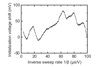
Figure D.1: Temperature fluctuations. Initialization voltage shift versus inverse sweep rate for the dataset depicted in Fig. 4 (a) ($U_{\mathrm{p}}=3.3$ V) of the main text. Each point corresponds to the measurement of the normalized squared return amplitude for a given inverse sweep rate. The first measurement is performed at 1/$\beta=100$ µs/V, representing the initialization at resonance frequency $\omega_{\mathrm{i}}(U_{\mathrm{i}})/2\pi$ for voltage $U_{\mathrm{i}}=10.4$ V. The implemented feedback loop regulates the initialization voltage in order to compensate the temperature fluctuations of the mechanical resonance. Consequently, the voltage shift illustrates the fluctuations of the ambient temperature.

Appendix E Experimental uncertainties

In Fig. E.1 we provide additional horizontal and vertical line-cuts from Fig. 3 of the main text. We observe pronounced oscillations in the normalized squared return amplitude (blue dots) as well as in the theoretically calculated return probability (red line). Nevertheless, the deviations between experiment and theory are more apparent, especially for Fig. E.1 (b), which depicts a vertical line-cut for a fixed inverse sweep rate of $1/\beta=60$ µs/V, i.e. within the ”plateau” in Fig. 3 (b) of the main text. Whereas the normalized squared return amplitude exhibits destructive interference, with the signal dropping close to zero, the minima in the return probability saturate at a value of approximately 0.3. This discrepancy is supposed to originate from the high sensitivity of the theoretical model to the input parameters. Experimental uncertainties and fluctuations deter the system from interference with the same constant parameters throughout all individual measurements. Since the ”plateau” in the theory is characteristic for a particular set of exact and constant parameters, it cannot be recovered under the given experimental conditions.

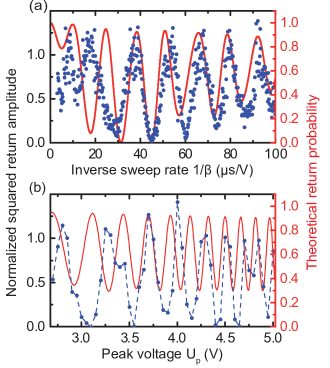
Figure E.1: Classical Stückelberg oscillations. (a) Normalized squared return amplitude (left axis, blue dots) and theoretically calculated return probability given by Eq. (9)  of the main text (right axis, red line) versus inverse sweep rate for a fixed peak voltage $U_{\mathrm{p}}=3.85$ V. (b) Same quantities as above but plotted as a function of peak voltage for a fixed inverse sweep rate $1/\beta=60$ µs/V. Blue dots are joined by blue dashed lines for illustration reasons.

The experimental uncertainties arise not solely from the temperature fluctuations. The voltage ramp also affects the characteristic parameters, such as the exact position of the avoided crossing $U_{\mathrm{a}}$. As previously stated, the dc voltage induces dipoles in the silicon nitride string resonator, which couple to the electric field gradient. A variation in dc voltage changes the inhomogeneous electric field at the same time, to which the nanoelectromechanical system needs to equilibrate. Consequently, the resonance frequencies of the mechanical modes drift towards the equilibrium position of the system. This drift, in turn, alters the characteristic system parameters, i.e. the characteristic voltages used for the theoretical calculations, and depends on the magnitude of the peak voltage $U_{\mathrm{p}}$. Concerning the initialization voltage, we simultaneously account for this effect via the initialization feedback loop (see section IV). Nevertheless, the exact position of the avoided crossing $U_{\mathrm{a}}$ varies slightly due to this retardation effect. Experimentally, we mitigate the influence of this drift by means of a ”thermalization” break of 10 seconds after each voltage ramp.
Another possible uncertainty arises from the imprecision in the value of the peak voltage $U_{\mathrm{p}}$ at the sample. The output amplitude uncertainty of the arbitrary function generator used in the room temperature experiments is classified by the manufacturer as $\pm$1 % of the nominal output voltage. Consequently, the maximum uncertainty in the peak voltage corresponds to $\pm$0.05 V for a maximum peak voltage of $U_{\mathrm{p}}=5.0$ V, which is equal to the voltage step size between two horizontal lines of Fig. 3 (a) in the main text.
As stated in the main text, we observed additional deviations in the experimental data of sample B from the theory for very fast voltage sweeps ($1/\beta\leq 50$ µs/V). These deviations originate from a flattening of the triangular voltage ramps. Records of the triangular voltage pulse taken by an oscilloscope revealed a flattening of the voltage apex depending on the peak voltage $U_{\mathrm{p}}$, which becomes significant for very fast sweeps. This flattening translates into a peak voltage cut-off and hence a different value of $U_{\mathrm{p}}$, which is transduced to the sample. We attribute this to the limited bandwidth of the summation amplifier, which reduces the pulse fidelity for very short ramp times. In the experiments conducted on sample A, a high performance summation amplifier has been employed together with a different arbitrary function generator. The latter exhibits a greatly enhanced bandwidth and sampling rate (nearly one order of magnitude) compared to the device employed in the room temperature experiment. As a consequence, the flattening of the voltage pulse apex is less pronounced and we find good agreement between the experimental data and the theory for inverse voltage sweep rates $1/\beta\leq 50$ µs/V.

References

- Stückelberg (1932) E. C. G. Stückelberg, “Theorie der unelastischen Stösse zwischen Atomen,” Helvetica Physica Acta 5, 369 (1932).
- Shevchenko et al. (2010) S. N. Shevchenko, S. Ashhab, and F. Nori, “Landau-Zener-Stückelberg interferometry,” Physics Reports 492, 1–30 (2010) .
- Yoakum et al. (1992) S. Yoakum, L. Sirko, and P. M. Koch, “Stueckelberg oscillations in the multiphoton excitation of helium Rydberg atoms: Observation with a pulse of coherent field and suppression by additive noise,” Physical Review Letters 69, 1919–1922 (1992).
- Mark et al. (2007) M. Mark, T. Kraemer, P. Waldburger, J. Herbig, C. Chin, H.-C. Nägerl, and R. Grimm, ““Stückelberg Interferometry” with Ultracold Molecules,” Physical Review Letters 99, 113201 (2007) .
- Dupont-Ferrier et al. (2013) E. Dupont-Ferrier, B. Roche, B. Voisin, X. Jehl, R. Wacquez, M. Vinet, M. Sanquer, and S. De Franceschi, “Coherent Coupling of Two Dopants in a Silicon Nanowire Probed by Landau-Zener-Stückelberg Interferometry,” Physical Review Letters 110, 136802 (2013).
- Wernsdorfer et al. (2000) W. Wernsdorfer, R. Sessoli, A. Caneschi, D. Gatteschi, and A. Cornia, “Nonadiabatic Landau-Zener tunneling in Fe8 molecular nanomagnets,” EPL (Europhysics Letters) 50, 552–558 (2000) .
- Petta et al. (2010) J. R. Petta, H. Lu, and A. C. Gossard, “A Coherent Beam Splitter for Electronic Spin States,” Science 327, 669– (2010) .
- Gaudreau et al. (2012) L. Gaudreau, G. Granger, A. Kam, G. C. Aers, S. A. Studenikin, P. Zawadzki, M. Pioro-Ladriere, Z. R. Wasilewski, and A. S. Sachrajda, “Coherent control of three-spin states in a triple quantum dot,” Nature Physics 8, 54–58 (2012).
- Ribeiro et al. (2013) H. Ribeiro, G. Burkard, J. R. Petta, H. Lu, and A. C. Gossard, “Coherent Adiabatic Spin Control in the Presence of Charge Noise Using Tailored Pulses,” Physical Review Letters 110, 086804 (2013) .
- Forster et al. (2014) F. Forster, G. Petersen, S. Manus, P. Hänggi, D. Schuh, W. Wegscheider, S. Kohler, and S. Ludwig, “Characterization of Qubit Dephasing by Landau-Zener-Stückelberg-Majorana Interferometry,” Physical Review Letters 112, 116803 (2014) .
- Oliver et al. (2005) W. D. Oliver, Y. Yu, J. C. Lee, K. K. Berggren, L. S. Levitov, and T. P. Orlando, “Mach-Zehnder Interferometry in a Strongly Driven Superconducting Qubit,” Science 310, 1653–1657 (2005) .
- Sillanpää et al. (2006) M. Sillanpää, T. Lehtinen, A. Paila, Y. Makhlin, and P. Hakonen, “Continuous-Time Monitoring of Landau-Zener Interference in a Cooper-Pair Box,” Physical Review Letters 96, 187002 (2006) .
- Lahaye et al. (2009) M. D. Lahaye, J. Suh, P. M. Echternach, K. C. Schwab, and M. L. Roukes, “Nanomechanical measurements of a superconducting qubit,” Nature 459, 960–964 (2009).
- Shevchenko et al. (2012) S. N. Shevchenko, S. Ashhab, and F. Nori, “Inverse Landau-Zener-Stückelberg problem for qubit-resonator systems,” Physical Review B 85, 094502 (2012) .
- Gong et al. (2016) M. Gong, Y. Zhou, D. Lan, Y. Fan, J. Pan, H. Yu, J. Chen, G. Sun, Y. Yu, S. Han, and P. Wu, “Landau-Zener-Stückelberg-Majorana interference in a 3D transmon driven by a chirped microwave,” Applied Physics Letters 108, 112602 (2016) .
- Heinrich et al. (2010) G. Heinrich, J. G. E. Harris, and F. Marquardt, “Photon shuttle: Landau-Zener-Stückelberg dynamics in an optomechanical system,” Physical Review A 81, 011801 (2010) .
- Vitanov and Garraway (1996) N. V. Vitanov and B. M. Garraway, “Landau-Zener model: Effects of finite coupling duration,” Physical Review A 53, 4288–4304 (1996).
- Landau (1932) L. D. Landau, “Zur Theorie der Energieübertragung. II,” Physics of the Soviet Union 2, 46 (1932).
- Zener (1932) C. Zener, “Non-Adiabatic Crossing of Energy Levels,” Proceedings of the Royal Society of London Series A 137, 696–702 (1932).
- Majorana (1932) E. Majorana, “Atomi orientati in campo magnetico variabile,” Nuovo Cimento 9, 43 (1932).
- Okamoto et al. (2013) H. Okamoto, A. Gourgout, C.-Y. Chang, K. Onomitsu, I. Mahboob, E. Y. Chang, and H. Yamaguchi, “Coherent phonon manipulation in coupled mechanical resonators,” Nature Physics 9, 480–484 (2013) .
- Faust et al. (2013) T. Faust, J. Rieger, M. J. Seitner, J. P. Kotthaus, and E. M. Weig, “Coherent control of a classical nanomechanical two-level system,” Nature Physics 9, 485–488 (2013) .
- Shkarin et al. (2014) A. B. Shkarin, N. E. Flowers-Jacobs, S. W. Hoch, A. D. Kashkanova, C. Deutsch, J. Reichel, and J. G. E. Harris, “Optically Mediated Hybridization between Two Mechanical Modes,” Physical Review Letters 112, 013602 (2014) .
- Faust et al. (2012a) T. Faust, J. Rieger, M. J. Seitner, P. Krenn, J. P. Kotthaus, and E. M. Weig, “Nonadiabatic Dynamics of Two Strongly Coupled Nanomechanical Resonator Modes,” Physical Review Letters 109, 037205 (2012a) .
- Maris and Xiong (1988) H. J. Maris and Q. Xiong, “Adiabatic and nonadiabatic processes in classical and quantum mechanics,” American Journal of Physics 56, 1114–1117 (1988).
- Shore et al. (2009) B. W. Shore, M. V. Gromovyy, L. P. Yatsenko, and V. I. Romanenko, “Simple mechanical analogs of rapid adiabatic passage in atomic physics,” American Journal of Physics 77, 1183–1194 (2009).
- Sun et al. (2011) G. Sun, X. Wen, B. Mao, Y. Yu, J. Chen, W. Xu, L. Kang, P. Wu, and S. Han, “Landau-Zener-Stückelberg interference of microwave-dressed states of a superconducting phase qubit,” Physical Review B 83, 180507 (2011) .
- Lohse et al. (2016) M. Lohse, C. Schweizer, O. Zilberberg, M. Aidelsburger, and I. Bloch, “A Thouless quantum pump with ultracold bosonic atoms in an optical superlattice,” Nature Physics 12, 350–354 (2016).
- Kaufman et al. (2016) A. M. Kaufman, M. E. Tai, A. Lukin, M. Rispoli, R. Schittko, P. M. Preiss, and M. Greiner, “Quantum thermalization through entanglement in an isolated many-body system,” ArXiv e-prints (2016), arXiv:1603.04409 [quant-ph] .
- Neuzner et al. (2016) A. Neuzner, M. Körber, O. Morin, S. Ritter, and G. Rempe, “Interference and dynamics of light from a distance-controlled atom pair in an optical cavity,” Nature Photonics 10, 303–306 (2016).
- Rieger et al. (2012) J. Rieger, T. Faust, M. J. Seitner, J. P. Kotthaus, and E. M. Weig, “Frequency and Q factor control of nanomechanical resonators,” Applied Physics Letters 101, 103110 (2012) .
- Faust et al. (2012b) T. Faust, P. Krenn, S. Manus, J. P. Kotthaus, and E. M. Weig, “Microwave cavity-enhanced transduction for plug and play nanomechanics at room temperature,” Nature Communications 3, 728 (2012b) .
- Novotny (2010) L. Novotny, “Strong coupling, energy splitting, and level crossings: A classical perspective,” American Journal of Physics 78, 1199–1202 (2010).
- Arnold (1989) V.I. Arnold, Mathematical Methods of Classical Mechanics, 2nd ed., Part III, Chapter 8, section 38 (Springer, 1989).
- Seitner et al. (2016) M. J. Seitner, H. Ribeiro, J. Kölbl, T. Faust, J. P. Kotthaus, and E.M. Weig, “Finite time Stückelberg interferometry in nanomechanics,” In preparation (2016).
- Usuki (1997) T. Usuki, “Theoretical study of Landau-Zener tunneling at the M+N level crossing,” Physical Review B 56, 13360–13366 (1997).
- Xu et al. (2016) H. Xu, D. Mason, L. Jiang, and J. G. E. Harris, “Topological energy transfer in an optomechanical system with exceptional points,” ArXiv e-prints (2016), arXiv:1602.06881 [physics.optics] .
- Rossi et al. (2016) N. Rossi, F. R. Braakman, D. Cadeddu, D. Vasyukov, G. Tütüncüoglu, A. F. i Morral, and M. Poggio, “Vectorial scanning force microscopy using a nanowire sensor,” ArXiv e-prints (2016), arXiv:1604.01073 [cond-mat.mes-hall] .
- Mercier de Lépinay et al. (2016) L. Mercier de Lépinay, B. Pigeau, B. Besga, P. Vincent, P. Poncharal, and O. Arcizet, “Universal Vectorial and Ultrasensitive Nanomechanical Force Field Sensor,” ArXiv e-prints (2016), arXiv:1604.01873 [cond-mat.mes-hall] .
- Andrews et al. (1997) MR Andrews, CG Townsend, H-J Miesner, DS Durfee, DM Kurn, and W Ketterle, “Observation of interference between two bose condensates,” Science 275, 637–641 (1997).
- Castin and Dalibard (1997) Yvan Castin and Jean Dalibard, “Relative phase of two bose-einstein condensates,” Physical Review A 55, 4330 (1997).
- Kohstall et al. (2011) C. Kohstall, S. Riedl, E. R. Sánchez Guajardo, L. A. Sidorenkov, J. Hecker Denschlag, and R. Grimm, “Observation of interference between two molecular Bose-Einstein condensates,” New Journal of Physics 13, 065027 (2011) .
- Maillet et al. (2015) O. Maillet, F. Vavrek, A. D. Fefferman, O. Bourgeois, and E. Collin, “Classical decoherence in a nanomechanical resonator,” ArXiv e-prints (2015), arXiv:1511.02120 [cond-mat.mes-hall] .