Lensing-induced morphology changes in CMB temperature maps in modified gravity theories

Abstract

Lensing of the Cosmic Microwave Background (CMB) changes the morphology of pattern of temperature fluctuations, so topological descriptors such as Minkowski Functionals can probe the gravity model responsible for the lensing. We show how the recently introduced two-to-two and three-to-one kurt-spectra (and their associated correlation functions), which depend on the power spectrum of the lensing potential, can be used to probe modified gravity theories such as $f({R})$ theories of gravity and quintessence models. We also investigate models based on effective field theory, which include the constant-$\Omega$ model, and low-energy Hořava theories. Estimates of the cumulative signal-to-noise for detection of lensing-induced morphology changes, reaches ${\cal O}(10^{3})$ for the future planned CMB polarization mission COrE⁺. Assuming foreground removal is possible to $\ell_{max}=3000$, we show that many modified gravity theories can be rejected with a high level of significance, making this technique comparable in power to galaxy weak lensing or redshift surveys. These topological estimators are also useful in distinguishing lensing from other scattering secondaries at the level of the four-point function or trispectrum. Examples include the kinetic Sunyaev-Zel’dovich (kSZ) effect which shares, with lensing, a lack of spectral distortion. We also discuss the complication of foreground contamination from unsubtracted point sources.

1 Introduction

The all-sky multi-frequency Cosmic Microwave Background (CMB) missions, such as WMAP, Planck[1] and further in future the proposed Experimental Probe of Inflationary Cosmology (EPIC) survey or ESAs Cosmic Origin Explorer (COrE, [2]), a fourth generation CMB satellite mission concept, are very important in furthering our knowledge of the Universe. The current generation of ground-based observations, namely the Atacama Cosmology Telescope (ACT; see ref.[4] for ACTPol) as well as the South Pole Telesecope (SPT; see ref.[5] for SPTPol) are already providing important clues especially of the CMB secondary anisotropy at smaller angular scales, below a few arc minutes. Secondary anisotropies, such as the thermal Sunyaev-Zel’dovich (tSZ) effect and Integrated Sachs-Wolfe (ISW) effect, tell us about the low-redshift Universe and can be a valuable source of cosmological information. In this paper, we focus on another secondary effect, the gravitational lensing of the CMB by the intervening matter. On the one hand, lensing is a source of nuisance for probing $B$-mode polarization arising from inflationary gravity waves[7, 6], but on the other hand, lensing of the CMB allows us to probe the matter distribution at an intermediate redshift ($z\approx 2$), beyond the typical reach of galaxy lensing surveys. The study of CMB lensing can tighten constraints on the contents and dynamics of the Universe, including the dark energy equation of state, neutrino mass hierarchy [8, 9, 10, 11] and modified theories of gravity [12]. It is the last effect that is the subject of this paper.

Lensing does not change the total power, but it redistributes power preferentially towards smaller angular scale [13], and the effects are most prominent below a few arc minutes. It is challenging to detect since the lensed field has the same spectrum as the unlensed CMB, and detection through the angular power spectrum is difficult. There are other ways to detect the lensing signal, for example through cross-correlation with external data sets[15, 14], and more recently internally using CMB data alone [18, 16, 17], and the most recent results from the Planck collaboration include a $40\sigma$ detection of the lensing potential[19]. The lensing has a quantitatively similar effect on CMB polarization spectra which may however be significant at larger angular scales for magnetic or $B$-mode polarization and is of considerable observational interest [20, 21]; a map of $B$-mode polarization has recently been released [22].

In addition to introducing a characteristic $B$-mode polarization, lensing generates secondary non-Gaussianity (non-Gaussianity) in temperature and polarization. While primordial non-Gaussianity can help to constrain inflation theory[23], similar studies for secondaries can provide useful clues to structure formation scenarios. In the absence of any frequency information, information from non-Gaussianity is helpful in separating out lensing. Early works in this area were carried out in real-space [24, 26, 25] or in the harmonic domain using multispectra [28, 27]. In the case of an ideal experiment, with infinite resolution, one-point statistics such as the PDF, lower-order moments will not change due to lensing. This too is related to the fact that lensing does not create power but simply redistributes it. However, experimental beam smoothing, or any other artificial smoothing, can introduce non-Gaussianity in even multispectra. For a Gaussian lensing potential, non-Gaussianity is introduced by lensing alone only the trispectrum at lowest order, whereas coupling of lensing with secondary anisotropies such as the ISW and SZ effects induces a non-zero bispectrum[31, 32, 29, 30].

Minkowski Functionals (MFs) are morphological descriptors that are commonly used in studying non-Gaussianity in cosmological datasets [33, 34]. In the CMB, they have already been applied for the analysis of WMAP 3-year data [35], Boomerang [36], and more recently to WMAP 7-year data [37]. These studies use a perturbative expansion to express MFs in terms of the multi-spectra [38]. In general the MFs can be expressed as a function of one-point (generalised) skewness parameters or their higher order analogues. In recent papers the concept of one-point moments such as skewness and kurtosis, was generalised to related power-spectra, skew-spectra and kurt-spectra, which carry more information[40, 39, 41]. This extra information is valuable in separating out individual contributions to the MFs at a given order, as well as to keep a control on systematics. The aim of this paper is to extend the results of recent work [42, 43] where lensing-induced mode-coupling of the lensing potential and secondaries were considered, as well as their effect on the morphology of CMB maps to the next order, i.e. to the level of the trispectrum. In this paper, we apply these statistics to study their ability to constrain modified gravity (MG) theories and the dark energy (DE) equation of state. For motivation and other cosmological probes of MG theories [see e.g. ref. 44, and references therein].

Following ref.[45], we will generalise the concept of kurt-spectrum and show how they can be used to reconstruct the MFs up to the fourth order. Kurt-spectra are useful as they can be used to separate lensing from the other secondaries such as the kinetic Sunyaev-Zel’dovich (kSZ) effect [46]. Similar analysis for frequency-cleaned tSZ maps and weak lensing observations were recently reported in ref.[47] and ref.[48] respectively. Reconstructing MFs from individual contributions is also important from a different perspective: the MFs are model-independent statistics and hence care must be taken to avoid any serendipitous detection from yet unexplored source of non-Gaussianity. Throughout, we will use spherical harmonics as basis as lensing of CMB is sensitive to lensing potential fluctuations at large angular scale $\ell<100$ and high $\ell$ (Limber’s) approximation is not adequate.

This paper is organized as follows. In §2 we review modified theories of gravity in the context of Effective Field Theory. In §3 we discuss the theoretical aspects of lensing-induced secondary non-Gaussianity in CMB maps. In §4 we provide details of MFs and related kurt-spectra for CMB lensing. In §5 estimators are developed, that can work with realistic mask, noise and beam. Finally §6 is reserved for discussion of our results and the conclusions are presented in §7. In Appendix A we provide explicit derivations of the two estimators as well as their Gaussian counterparts. In Appendix B we show how the one-point kurtosis are recovered from both kurt-spectra. In Appendix C we discuss the possibility of constructing sub-optimal estimators for lensing reconstruction.

2 Modified Gravity Scenarios in an Effective Field Theory Framework

The effective field theory (EFT) approach to dark energy/modified gravity (DE/MG) was recently proposed  [50, 49]. An action is built in the Jordan frame and unitary gauge by considering the operators which are invariant under time-dependent spatial diffeomorphisms. It is able to unify all of the viable single scalar field theories of DE/MG which have a well defined Jordan frame representation, such as $f(R)$ gravity, quintessence, Horndeski models, etc. (see ref.[51] for a review of the models). In this approach, the additional scalar degree of freedom representing DE/MG is eaten by the metric via a foliation of space-time into space-like hyper-surfaces. Up to the quadratic order, the action reads

$$\mathcal{S}_{\rm EFT}=\int d^{4}x \sqrt{-g}\bigg{\{}\frac{m_{0}^{2}}{2}\left[1+\Omega(\tau)\right]R+\Lambda(\tau)-c(\tau)\,a^{2}\delta g^{00}{}$$

$$+\frac{M_{2}^{4}(\tau)}{2}\left(a^{2}\delta g^{00}\right)^{2}-\frac{\bar{M}_{1}^{3}(\tau)}{2}\,a^{2}\delta g^{00}\,\delta\tensor{K}{{}^{\mu}_{\mu}}-\frac{\bar{M}_{2}^{2}(\tau)}{2}\left(\delta\tensor{K}{{}^{\mu}_{\mu}}\right)^{2}$$

$$-\frac{\bar{M}_{3}^{2}(\tau)}{2}\,\delta\tensor{K}{{}^{\mu}_{\nu}}\,\delta\tensor{K}{{}^{\nu}_{\mu}}+m_{2}^{2}(\tau)\left(g^{\mu\nu}+n^{\mu}n^{\nu}\right)\partial_{\mu}(a^{2}g^{00})\partial_{\nu}(a^{2}g^{00})$$

$$+\frac{\hat{M}^{2}(\tau)}{2}\,a^{2}\delta g^{00}\,\delta\mathcal{R}+\ldots\bigg{\}}+S_{m}[g_{\mu\nu},\chi_{m}],$$ (2.1)

where $R$ is the four-dimensional Ricci scalar, $\delta g^{00}$, $\delta\tensor{K}{{}^{\mu}_{\nu}}$, $\delta\tensor{K}{{}^{\mu}_{\mu}}$ and $\delta\mathcal{R}$ are respectively the perturbations of the upper time-time component of the metric, the extrinsic curvature and its trace and the three dimensional spatial Ricci scalar. Finally, $S_{m}$ is the matter action. Since the choice of the unitary gauge breaks time diffeomorphism invariance, each operator in the action can be multiplied by a time-dependent coefficient; in our convention, $\{\Omega,\Lambda,c,M_{2}^{4},\bar{M}_{1}^{3},\bar{M}_{2}^{2},\bar{M}_{2}^{2},\bar{M}_{3}^{2},m_{2}^{2},\hat{M}^{2}\}$ are unknown functions of the conformal time, $\tau$, and we will refer to them as EFT functions. We can read that up to the quadratic order, we only have 9 functions. Furthermore, three of them, namely $\{\Omega,c,\Lambda\}$, are the only functions contributing both to the dynamics of the background and of the perturbations, while the others play a role only at level of perturbations. Due to the theoretical degeneracies at the kinematic background level, the philosophy of EFT is to fix the cosmic background evolution in a priori manner, then focus on the linear perturbation dynamics which are consistent with the given background history. Fixing the time evolution of $H(z)$ and $\dot{H}(z)$ helps us to reduce two of the background EFT functions, normally chosen to be $c,\Lambda$, thus reducing the total number of independent EFT functions to seven.

After writing down the generic formula Eq.(2.1), we can see that the only unknown parts of this action are these EFT functions. There are basically two ways to parametrize them, namely covariant mapping parametrization and phenomenological parametrization. The former one is suitable for studying well-known models, which are written in the covariant formalism, while the latter can be used to study the phenomenological models which are inspired by observation.

In the action Eq.(2.1), the extra scalar degree of freedom is hidden inside the metric perturbations. However, in order to study the dynamics of linear perturbations and investigate the stability of a given model, it is more convenient to make it explicit by means of the St$\ddot{\text{u}}$kelberg technique i.e. performing an infinitesimal coordinate transformation such that $\tau\rightarrow\tau+\pi$, where the new field $\pi$ is the St$\ddot{\text{u}}$kelberg field, which describes the extra propagating degree of freedom. Varying the action with respect to the $\pi$-field one obtains a dynamical perturbative equation for the extra degree of freedom which allows direct control of the stability of the theory, as discussed at length in ref. [52].

In refs. [52, 53] the EFT framework has been implemented into CAMB/CosmoMC [54, 55] creating the EFTCAMB/EFTCosmoMC patches, which are publicly available (see ref. [56] for technical details). EFTCAMB evolves the full equations for linear perturbations without relying on any quasi-static approximation. In addition to the standard matter components (i.e. dark matter, baryon, radiation and massless neutrinos), massive neutrinos have also been included [57]. As mentioned above, EFTCAMB allows the study of perturbations in a phenomenological way (usually referred to as pure EFT mode), investigating the cosmological implications of the different operators in action Eq.(2.1). It can also be used to study the exact dynamics for specific models, after the mapping of the given model into the EFT language has been worked out (usually referred to as mapping mode). In the latter case one can treat the background via a designer approach, i.e. fixing the expansion history and reconstructing the specific model in terms of EFT functions; or full mapping approach, i.e. one can solve the full background and linear perturbation equations of a particular model. Furthermore, the code has a powerful built-in module that investigates whether a chosen model is viable, through a set of general conditions of mathematical and physical stability. In particular, the physical requirements include the avoidance of ghost and gradient instabilities for both the scalar and the tensor degrees of freedom. The stability requirements are translated into viability priors on the parameter space when using EFTCosmoMC to interface EFTCAMB with cosmological data, and they can sometimes dominate over the constraining power of data [53].

In this paper, we select a few models both from the pure EFT mode and also mapping mode described above. We choose, for the former, the constant-$\Omega$ [58] models, and for the latter, the designer quintessence [56], $f(R)$ model [59, 52] and low-energy Hořava gravity [60, 61]. In the rest part of this section, we will briefly describe these models.

2.1 Pure EFT models

For the pure EFT models, we select the constant-$\Omega$ model, which consist in taking a constant value for the conformal coupling $\Omega(a)=\Omega_{0}^{\rm EFT}$ and requiring the expansion history to be exactly that of the $\Lambda$CDM model. This requirement will then fix, through the Friedmann equations, the time dependence of the operators $c$ and $\Lambda$. We emphasize here that the constant-$\Omega$ model is not a simple redefinition of the gravitational constant. In fact the requirement of having a $\Lambda$CDM background with a non-vanishing $\Omega$, that would change the expansion history, means that a scalar field is sourced in order to compensate this change. This scalar field will then interact with the other matter fields and modify the behaviour of cosmological perturbations and consequently the CMB power spectra and the growth of structure. For instance, it is easy to show that in the constant-$\Omega$ model, $c(\tau)=\Omega(\rho_{m}+P_{m})/2$, which is vanishing in general relativity, is non-zero.

Another general remark we would like to make on the models that we consider here, is that they display a radically different cosmology, as they correspond to two different behaviours of the perturbation’s effective gravitational constant. Viable models, in the $f(R)$ case, correspond to an enhancement of the gravitational constant which in turn results in the amplification of the growth of structure that enhances substantially the lensing of the CMB. In the constant-$\Omega$ model, if $\Omega$ is negative, the model will have an enhanced effective gravitational constant with a phenomenology similar to that of $f(R)$ models. Hereafter, we dubbed it as “${\rm EFT}_{1}$”. On the other hand, if $\Omega$ is positive the model will be characterized by a smaller effective gravitational constant resulting in a suppression of the growth and consequently a suppression of the CMB lensing. In this paper, we dubbed it as “${\rm EFT}_{2}$”. In details, we fix $\Omega_{0}^{\rm EFT}=-0.1$ and $+0.1$ for “${\rm EFT}_{1}$” and “${\rm EFT}_{2}$”, respectively.

2.2 Mapping models

For the mapping models, we select three models, namely the designer quintessence, $f(R)$ model and low-energy Hořava gravity. As demonstrated above, one of the advantages of the EFT approach is its ability to unify the languages which describe the linear dynamics of most of the viable single scalar field DE/MG models.

Via the mapping procedure, we are allowed to design the functional form of the quintessence potential (with canonical kinetic term) to reproduce the input background evolution. Generally speaking, in the minimally-coupled quintessence model, the effect on the growth factor from the quintessence field is sub-dominant compared with its modification to the background expansion. Physically, this is because the Jeans length of the quintessence field is a super-horizon scale, so, there is no significant clustering effect from the scalar degree of freedom. We suggest ref.[56] for readers who are interested in the details of this model. In the following calculation, we fix $w_{0}=-0.9$ and $w_{a}=0.25$ and refer to it as the “Q” model.

On the other hand, in the $f(R)$ gravity, the linear perturbation dynamics are more important than its background kinematics. This is because the effective gravitational constant is enhanced by a factor $4/3$ on the scales which are smaller than the Compton wavelength, $B_{0}\sim 6f_{RR}H^{2}/(1+f_{R})$, of the scalar field. This will magnify the lensing effect significantly, as we will show later. In the following calculation, we fix $B_{0}=0.1$.

The last modified gravity models we selected are the low-energy Hořava models. The basic model was first proposed in ref.[60] to solve the UV complete problem of quantum gravity, then it was embedded in the EFT approach in ref.[61] to study cosmic late-time acceleration. Basically, its phenomenology on the background is simply rescaling the Hubble parameter; and on the perturbation level, due to the strong coupling with the gravity sector, the scalar field perturbations could suppress the linear structure formation rate substantially. In this paper, we select two Hořava models, one with three parameters ($\lambda=1.4$, $\xi=0.9$, $\eta=1.0$), the other with two ($\lambda=1.4$, $\eta=1.0$). Hereafter, we dubbed them as “${\rm H}_{3}$” and “${\rm H}_{2}$” models, respectively. Compared with the “${\rm H}_{3}$” model, the “${\rm H}_{2}$” are designed to evade the PPN constraint.

Finally, we take the $\Lambda$CDM model (“$\Lambda$”) as the baseline model, and all the vanilla cosmological parameters are the same as the ones from the Planck-2015 [62] data release.

3 Lensing induced non-Gaussianity in CMB Temperature Maps

In this section we will briefly review certain aspects of lensing of the CMB [63, 64, 27]. For a full review see ref.[13].

3.1 Lensing in Temperature Maps

In the context of CMB lensing, the surface of last scattering can be thought of as a single source plane. The projected lensing potential $\phi({\hat{\Omega}})$ towards an angular direction ${\hat{\Omega}}=(\theta,\phi)$ can be expressed in terms of a line of sight integration of the 3D potential $\Phi({\bf r})=\Phi(r,{\hat{\Omega}})$:

$$\phi({\hat{\Omega}})=-2\int_{0}^{r_{0}}dr{{d_{A}(r-r)}\over d_{A}(r)d_{A}(r_{0})}\Phi(r,{\hat{\Omega}}).$$ (3.1)

Here $r_{0}$ is the comoving conformal distance to the surface of last scattering and $d_{A}(r)$ is the comoving angular diameter distance out to $r$. Lensing effectively redistributes the temperature $\Theta({\hat{\Omega}})=[\delta T({\hat{\Omega}})/T_{0}]$ on the surface of the sky through the angular deflections resulting along the photon path, $\alpha({\hat{\Omega}})=\nabla\phi({\hat{\Omega}})$ such that $\Theta({\hat{\Omega}})=\bar{\Theta}({\hat{\Omega}}+\alpha)$, where $\Theta$ is the lensed CMB sky and $\bar{\Theta}$ corresponds to the temperature distribution in the absence of lensing, and $\nabla$ is the covariant derivative on the surface of the unit sphere. For the following discussion we will ignore the secondary contribution. Coupling of lensing with secondaries and resulting impact on morphological properties of CMB maps have been discussed in detail in [42]. Expanding the above expression in a Taylor series we can write [31, 32]:

$$\Theta({\hat{\Omega}})=\bar{\Theta}({\hat{\Omega}}+\alpha)\approx\bar{\Theta}({\hat{\Omega}})+\nabla_{i}\phi({\hat{\Omega}})\nabla^{i}\bar{\Theta}({\hat{\Omega}})+{\cal O}(\phi^{2});$$ (3.2)

$$\delta\Theta({\hat{\Omega}})=\Theta({\hat{\Omega}})-\bar{\Theta}({\hat{\Omega}})\approx\nabla_{i}\phi({\hat{\Omega}})\nabla^{i}\bar{\Theta}({\hat{\Omega}}).$$ (3.3)

In the harmonic domain, using spherical harmonics $Y_{lm}({\hat{\Omega}})$ as the basis function, we can express the multipole of lensing induced temperature anisotropy $\delta\Theta_{lm}$ in terms of multipoles of lensing potential $\phi_{LM}$ and multipole of the unlensed CMB temperature anisotropy $\bar{\Theta}_{lm}$ respectively:

$$\delta\Theta_{\ell m}=\int d{\hat{\Omega}}Y^{*}_{\ell m}({\hat{\Omega}})\nabla_{i}\phi({\hat{\Omega}})\nabla^{i}\bar{\Theta}({\hat{\Omega}}){}$$

$$=\int d{\hat{\Omega}}Y^{*}_{\ell m}({\hat{\Omega}})\nabla_{i}\left[\sum_{LM}\phi_{LM}Y^{*}_{LM}({\hat{\Omega}})\right]\nabla^{i}\left[\sum_{\ell^{\prime}m^{\prime}}\bar{\Theta}_{\ell^{\prime}m^{\prime}}Y^{*}_{\ell^{\prime}m^{\prime}}({\hat{\Omega}})\right]{}$$

$$=\sum_{LM}\sum_{\ell^{\prime}m^{\prime}}(-1)^{m}\phi_{LM}\bar{\Theta}_{\ell^{\prime}m^{\prime}}\;{}_{0}F_{\ell\ell^{\prime}L}\left(\begin{array}[]{ c c c }\ell&\ell^{\prime}&L\\ m&-m^{\prime}&-M\end{array}\right);$$ (3.6)

where we have used the Gaunt integral [65] to arrive at the last line. The following notations were introduced:

$${}_{\pm s}F_{\ell L\ell^{\prime}}\equiv{1\over 2}{}_{\pm s}I_{\ell\ell^{\prime}L}\Lambda_{\ell\ell^{\prime}L}={1\over 2}{}_{\pm s}I_{\ell\ell^{\prime}L}[\Pi_{L}+\Pi_{\ell^{\prime}}-\Pi_{\ell}];\quad$$ (3.7)

$${}_{\pm s}I_{\ell\ell^{\prime}L}=\sqrt{\Pi_{\ell}\Pi_{\ell^{\prime}}\Pi_{L}\over 4\pi}\left(\begin{array}[]{ c c c }\ell&\ell^{\prime}&L\\ \pm s&\mp s&0\end{array}\right),$$ (3.10)

where $\Pi_{\ell}\equiv\ell(\ell+1)$ and the last matrix is a Wigner $3j$ symbol. The function ${}_{\pm s}F_{l_{1}Ll_{2}}$ encodes the rotationally-invariant part of the coupling between three multipoles $(l_{1},l_{2},L)$. To simplify our notation, as is common in the literature, we will denote ${}_{0}I_{\ell\ell^{\prime}\ell^{\prime\prime}}$ as $I_{\ell\ell^{\prime}\ell^{\prime\prime}}$ by dropping the $s$ index.

The analytical modelling of higher-order correlation functions is most naturally done in the harmonic domain where they are represented by the multi-spectra. It is known that lensing of CMB only induces even-order multi-spectra. Thus the lowest-order departure from Gaussianity, in case of CMB lensing, is characterized by the connected part of the four-point correlation function (or equivalently the trispectrum in the harmonic domain) defined through the relation:

$$\langle\Theta_{\ell_{1}m_{1}}\Theta_{\ell_{2}m_{2}}\Theta_{\ell_{3}m_{3}}\Theta_{\ell_{4}m_{4}}\rangle=\langle\Theta_{\ell_{1}m_{1}}\Theta_{\ell_{2}m_{2}}\Theta_{\ell_{3}m_{3}}\Theta_{\ell_{4}m_{4}}\rangle_{\rm c}+\langle\Theta_{\ell_{1}m_{1}}\Theta_{\ell_{2}m_{2}}\Theta_{\ell_{3}m_{3}}\Theta_{\ell_{4}m_{4}}\rangle_{\rm G};$$ (3.11)

where the subscripts _G and _c correspond to Gaussian and non-Gaussian (or connected) contributions to the four-point correlation function. The connected part of the four-point correlation function in real-space is related to the trispectrum $T^{\ell_{1}\ell_{2}}_{\ell_{3}\ell_{4}}(\ell)$ through the following relation:

$$\langle\Theta_{\ell_{1}m_{1}}\Theta_{\ell_{2}m_{2}}\Theta_{\ell_{3}m_{3}}\Theta_{\ell_{4}m_{4}}\rangle_{c}{}=$$

$$\sum_{\ell m}(-1)^{m}T^{\ell_{1}\ell_{2}}_{\ell_{3}\ell_{4}}(\ell)\left(\begin{array}[]{ c c c }\ell_{1}&\ell_{2}&\ell\\ m_{1}&-m_{2}&-m\end{array}\right)\left(\begin{array}[]{ c c c }\ell_{3}&\ell_{4}&\ell\\ m_{3}&-m_{4}&-m\end{array}\right).$$ (3.16)

To impose the symmetry inherent in the trispectrum it is expressed in terms of its “pairing matrix” $P^{\ell_{1}\ell_{2}}_{\ell_{3}\ell_{4}}(\ell)$.

$$T^{\ell_{1}\ell_{2}}_{\ell_{3}\ell_{4}}(\ell)=P^{\ell_{1}\ell_{2}}_{\ell_{3}\ell_{4}}(\ell) +\Xi_{\ell}\Big{[}\sum_{l^{\prime}}(-1)^{\ell_{2}+\ell_{3}}\left\{\begin{array}[]{ c c c }\ell_{1}&\ell_{2}&\ell\\ \ell_{4}&\ell_{3}&\ell^{\prime}\end{array}\right\}P^{\ell_{1}\ell_{3}}_{\ell_{2}\ell_{4}}(\ell^{\prime}){}$$ (3.22)

$$+\sum_{\ell^{\prime}}(-1)^{L+L^{\prime}}\left\{\begin{array}[]{ c c c }\ell_{1}&\ell_{2}&\ell\\ \ell_{3}&\ell_{4}&\ell^{\prime}\end{array}\right\}P^{\ell_{1}\ell_{4}}_{\ell_{3}\ell_{2}}(\ell^{\prime})\Big{]},$$

where $\Xi_{\ell}\equiv 2\ell+1$, and the matrices in curly brackets are Wigner $6j$-symbols which are defined in terms of $3j$ symbols (see ref.[65]). The “pairing matrix” can be further decomposed in terms of the reduced trispectrum $\tau^{\ell_{1}\ell_{2}}_{\ell_{3}\ell_{4}}(\ell)$:

$$P^{\ell_{1}\ell_{2}}_{\ell_{3}\ell_{4}}(\ell)=\tau^{\ell_{1}\ell_{2}}_{\ell_{3}\ell_{4}}(\ell)+(-1)^{\Sigma_{U}}\tau^{\ell_{2}\ell_{1}}_{\ell_{3}\ell_{4}}(\ell)+(-1)^{\Sigma_{L}}\tau^{\ell_{1}\ell_{2}}_{\ell_{4}\ell_{3}}(\ell)+(-1)^{\Sigma_{L}+\Sigma_{U}}\tau^{\ell_{2}\ell_{1}}_{\ell_{4}\ell_{3}}(\ell);{}$$

$$\quad\Sigma_{L}=\ell_{1}+\ell_{2}+\ell;\quad\Sigma_{U}=\ell_{3}+\ell_{4}+\ell.$$ (3.23)

In the case of weak lensing of CMB the reduced trispectrum $\tau$ depends only on the power-spectrum of the lensing potential ${\cal C}_{\ell}^{\phi\phi}=\langle\phi_{\ell m}\phi^{*}_{\ell m}\rangle$ and the power spectrum of temperature anisotropy ${\cal C}^{T}_{\ell}$:

$$\tau^{\ell_{1}\ell_{2}}_{\ell_{3}\ell_{4}}(\ell)={\cal C}_{\ell}^{\phi\phi}\bar{\cal C}^{T}_{\ell_{2}}\bar{\cal C}^{T}_{\ell_{4}}\;{}_{0}F_{\ell_{1}\ell\ell_{2}}\;{}_{0}F_{\ell_{3}\ell\ell_{4}}$$ (3.24)

Previous studies have already shown that the pairing matrix $P^{\ell_{1}\ell_{2}}_{\ell_{3}\ell_{4}}(\ell)$ can very accurately describe the trispectrum $\tau^{\ell_{1}\ell_{2}}_{\ell_{3}\ell_{4}}(\ell)$:

$$T^{\ell_{3}\ell_{4}}_{\ell_{1}\ell_{2}}(\ell)\approx P^{\ell_{3}\ell_{4}}_{\ell_{1}\ell_{2}}(\ell) = {\cal C}_{\ell}^{\phi\phi}\left(\bar{\cal C}^{T}_{\ell_{2}}{}_{0}F_{\ell_{1}\ell\ell_{2}}+\bar{\cal C}^{T}_{\ell_{1}}{}_{0}F_{\ell_{2}\ell\ell_{1}}\right)\left(\bar{\cal C}^{T}_{\ell_{4}}{}_{0}F_{\ell_{3}\ell\ell_{4}}+\bar{\cal C}^{T}_{\ell_{3}}{}_{0}F_{\ell_{4}\ell\ell_{3}}\right)$$ (3.25)

$$= {\cal C}_{\ell}^{\phi\phi}f_{\ell_{1}\ell\ell_{2}}f_{\ell_{3}\ell\ell_{4}}$$ (3.26)

This is the approximation which we will use in our study.

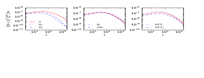
Figure 1: CMB Lensing potential power sepctrum ${\cal C}^{\phi\phi}_{\ell}$ as a function of $\ell$ for various Modified Gravity theories. In left panel we show two Hořava theories denoted as $\rm H_{2}$ (dot-dashed line) and $\rm H_{3}$ (dashed line). The standard $\Lambda$CDM prediction is depicted as a solid-line in each panel. In the middle panel we compare results for a quintessence model (dot-dashed) and $f(R)$ theory (dashed) results. In the right panel we show results from two different EFT caclulations EFT₁ (dot-dashed) and EFT₂ (dashed). See text for more details.

3.2 Gaussian Component

The Gaussian component of the four-point correlation function defined in Eq.(3.11) can also be expressed as follows:

$$\langle\Theta_{\ell_{1}m_{1}}\Theta_{\ell_{2}m_{2}}\Theta_{\ell_{3}m_{3}}\Theta_{\ell_{4}m_{4}}\rangle_{\rm G}{}$$

$$=\sum_{\ell m}(-1)^{m}G_{\ell_{3}\ell_{4}}^{\ell_{1}\ell_{2}}(\ell)\left(\begin{array}[]{ c c c }\ell_{1}&\ell_{2}&\ell\\ m_{1}&-m_{2}&-m\end{array}\right)\left(\begin{array}[]{ c c c }\ell_{3}&\ell_{4}&\ell\\ m_{3}&-m_{4}&-m\end{array}\right)$$ (3.31)

The Gaussian component of the trispectrum defined above $G^{{\ell}_{1}{\ell}_{2}}_{{\ell}_{3}{\ell}_{4}}({\ell})$ representing the disjoint contribution to our-point correlation function is determined completely by the (unlensed) CMB power spectrum $\bar{\cal C}_{\ell}^{T}$:

$$G^{\ell_{1}\ell_{2}}_{\ell_{3}\ell_{4}}(\ell) = (-1)^{\ell_{2}+\ell_{3}}\sqrt{\Xi_{\ell_{1}}\Xi_{\ell_{3}}}{\cal C}^{T}_{\ell_{1}}{\cal C}^{T}_{\ell_{3}}\delta_{\ell_{1}\ell_{3}}\delta_{\ell_{2}\ell_{4}}\delta_{\ell 0}{}$$ (3.32)

$$+\Xi_{\ell}\;{\cal C}^{T}_{\ell_{1}}{\cal C}^{T}_{\ell_{2}}\left[(-1)^{\ell_{1}+\ell_{2}+\ell}\delta_{\ell_{1}\ell_{3}}\delta_{\ell_{2}\ell_{4}}+\delta_{\ell_{1}\ell_{4}}\delta_{\ell_{2}\ell_{3}}\right]$$

Henceforth, we will ignore the $\ell=0$ mode as it does not contribution to the deflection of photons.

3.3 Foregrounds

In addition to cosmological sources of non-Gaussianity both primary and secondary, foreground such as the unsubtracted point-sources can also make a significant contribution.

The bispectrum and trispectrum from extragalactic radio and infra-red sources with fluxes ${F}$ smaller than a certain detection threshold ${F}_{\rm d}$ is simple to estimate if Poisson distributed. The trispectrum for the unsubtracted point source distribution then has a constant amplitude $t_{\rm ps}$:

$$T^{\ell_{3}\ell_{4}}_{\ell_{1}\ell_{2}}(\ell)=t_{\rm ps}\,I_{\ell_{1}\ell_{2}\ell}I_{\ell_{3}\ell_{4}\ell}.$$ (3.33)

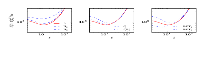
Figure 2: CMB temperature power spectra for the models shown in Figure-1. The line styles representing various models remain the same.

Following the procedure outlines in ref.[23] we obtain the following expression for $t^{\rm ps}$:

$$t_{\rm ps}={(2-\beta)^{2}\over\beta(4-\beta)}[n(<{F}_{\rm d})]^{-1}[{\cal C}_{\rm ps}]^{2}.$$ (3.34)

Here ${\cal C}_{\rm ps}$ is the $\ell$ independent power spectrum for the point sources which has the following expression:

$${\cal C}_{\rm ps}=g^{2}(x){\beta\over 2-\beta}n(<{F}_{\rm d}){F}_{\rm d}^{2}.$$ (3.35)

Here $d{\rm n}/d{\rm F}$ is the differential source count per unit solid angle and we have defined $n(<F_{d})=\int_{0}^{F_{d}}d{F}{d{\rm n}/d{F}}$. It is generally assumed to be a power-law, $dn/{dF}\propto{F}^{-\beta-1}$. For example, for Euclidean source counts $\beta=3/2$. We have defined $x={h\nu/k_{B}{\rm T}}\approx(\nu/56.80{\rm GHz})({\rm T}/2.726)^{-1}$ and $g(x)=2\,(hc)^{2}/({k_{B}\rm T})^{3}[{\rm sinh}(x/2)/x^{2}]^{2}$. For the 217 GHz assuming $n(<{F}_{\rm d})=100$ we obtain $t_{\rm ps}\approx 2\times 10^{-38}$ and for $90$ GHz assuming $n(<{F}_{d})=7$ we get $t_{\rm ps}\approx 2\times 10^{-34}$. These results should only be considered a very crude order of magnitude estimates.

4 Morphological Estimators

We outline our estimators in this section and relate them to morphological statistics such as the Minkowski Functionals.

4.1 Minkowski Functionals

The MFs are well known morphological descriptors which are used in the study of random fields. Morphological properties are the properties that remain invariant under rotation and translation (see ref.[66] for more formal introduction). They are defined over an excursion set $\Sigma$ for a given threshold $\nu$. The three MFs that we will use for two dimensional (2D) temperature anisotropy $\Theta({\hat{\Omega}})$ defined on the surface of the sky can be expressed as:

$${\cal V}_{0}(\nu)=\int_{\Sigma}da;\quad{\cal V}_{1}(\nu)={1\over 4}\int_{\partial\Sigma}dl;\quad{\cal V}_{2}(\nu)={1\over 2\pi}\int_{\partial\Sigma}\kappa dl;\quad\nu={\Theta\over\sigma_{0}}.$$ (4.1)

Here $da$, $dl$ are the elements for the excursion set $\Sigma$ and its boundary $\partial\Sigma$. The MFs ${\cal V}_{k}(\nu)$ correspond to the area of the excursion set $\Sigma$, the length of its boundary $\partial\Sigma$ as well as the integral curvature along its boundary which is related to the genus $g$ and hence the Euler characteristics $\chi$.

The MFs for a random Gaussian field are well known and given by Tomita’s formula [67] and are completely defined by the corresponding power spectrum ${\cal C}_{\ell}$. A perturbative analysis was suggested to go beyond the Gaussian distribution in ref.[38]:

$${\cal V}_{k}(\nu)={1\over(2\pi)^{(k+1)/2}}{\omega_{2}\over\omega_{2-k}\omega_{k}}\exp\left(-{\nu^{2}\over 2}\right)\left(\sigma_{1}\over\sqrt{2}\sigma_{0}\right)^{k}v_{k}(\nu);$$ (4.2)

$$v_{k}(\nu)=\left[v_{k}^{(0)}(\nu)+v_{k}^{(1)}(\nu)\sigma_{0}+v_{k}^{(2)}(\nu)\sigma_{0}^{2}+\cdots\right];$$ (4.3)

$$\sigma_{j}^{2}={1\over 4\pi}\sum_{\ell}\,\Xi_{\ell}\,\Pi_{\ell}^{j}\,{\cal C}_{\ell}b_{\ell}^{2}(\theta_{0});$$ (4.4)

$${\Pi}_{\ell}=\ell(\ell+1);\quad b_{\ell}(\theta_{0})=\exp\left[-\Pi_{\ell}{\theta_{b}^{2}}\right];\quad\theta_{b}={\theta_{0}\over\sqrt{16\ln 2}}.$$ (4.5)

$$H_{-1}(\nu)=\sqrt{\pi\over 2}e^{\nu^{2}/2}{\rm erfc}\left({\nu\over 2}\right);$$ (4.6)

$$H_{0}(\nu)=1;\quad H_{1}(\nu)=\nu;\quad H_{2}(\nu)=\nu^{2}-1;$$ (4.7)

$$H_{3}(\nu)=\nu^{3}-3\nu;\quad H_{4}(\nu)=\nu^{4}-6\nu^{2}+3;$$ (4.8)

$$H_{n}(\nu)=(-1)^{n}\exp\left({\nu^{2}\over 2}\right){d^{n}\over d\nu^{n}}\exp\left(-{\nu^{2}\over 2}\right).$$ (4.9)

We have assumed a Gaussian beam $b_{\ell}(\theta_{0})$ with FWHM $=\theta_{0}$. The constant $\omega_{k}$ introduced above is the volume of the unit sphere in k-dimension. $w_{k}={\pi^{k/2}/\Gamma(k/2+1)}$ in 2D we will only need $\omega_{0}=1$, $\omega_{1}=2$ and $\omega_{2}=\pi$. For a purely Gaussian distribution $v_{k}^{(0)}(\nu)=H_{k-1}(\nu)$ and all higher order terms vanish. We notice that $\sigma_{0}^{2}=\langle\delta\Theta^{2}\rangle$ and $\sigma_{1}^{2}=\langle|\nabla\Theta|^{2}\rangle$.

4.2 Kurtosis Spectra

The leading order terms that signify non-Gaussianity of MFs depend on the bispectrum or equivalently a set of three generalised skewness parameters. The next to the leading order order correction terms depend on a set of four generalised kurtosis parameters $K^{(i)}$ that are fourth order statistics. In general the kurtosis parameters are collapsed fourth order one-point cumulants and probe the trispectrum with varying weights [68]. The four different kurtosis parameters that are related to the MFs are a natural generalisation of the ordinary kurtosis $K^{(0)}$ which is routinely applied in many cosmological studies. We will denote these generalised kurtosis parameters by $K^{(i)};i=1,2,3$. These parameters are constructed from the derivative field of the original map $\Theta({\hat{\Omega}})$ and its derivatives $|\nabla_{i}\Theta({\hat{\Omega}})|^{2}=[\nabla_{i}\Theta({\hat{\Omega}})\nabla^{i}\Theta({\hat{\Omega}})]$ and $[\nabla^{2}\Theta({\hat{\Omega}})]$.

$$K^{(0)}\equiv{\langle\Theta^{4}\rangle_{c}\over\sigma_{0}^{6}};\quad K^{(1)}\equiv{\langle\Theta^{3}\nabla^{2}\Theta\rangle_{c}\over\sigma_{0}^{4}\sigma_{1}^{2}};\quad$$ (4.10)

$$K^{(2)}\equiv K^{(2a)}+K^{(2b)}\equiv 2{\langle\Theta|(\nabla\Theta)|^{2}(\nabla^{2}\Theta)\rangle_{c}\over\sigma_{0}^{2}\sigma_{1}^{4}}+{}{\langle|(\nabla\Theta)|^{4}\rangle_{c}\over\sigma_{0}^{2}\sigma_{1}^{4}};\quad K^{(3)}\equiv{\langle|\nabla\Theta|^{4}\rangle_{c}\over 2\sigma_{0}^{2}\sigma_{1}^{4}}.$$ (4.11)

The subscript _c correspond to the connected components which indicates that all Gaussian unconnected contributions are subtracted out, these include both noise as well as the signal contribution.

If we ignore lensing-secondary coupling contributions discussed in ref.[42] and contribution from primordial non-Gaussianity[68], the next-to-leading order corrections to the MFs involve tri-spectral contributions $K^{(i)}$s which can be derived following ref.[38].

$$v_{0}^{(4)}(\nu)={K^{(0)}\over 24}{\cal H}_{3}(\nu);\quad$$ (4.12)

$$v_{1}^{(4)}(\nu)={K^{(0)}\over 24}{\cal H}_{4}(\nu)-{K^{(1)}\over 12}{\cal H}_{2}(\nu)-{K^{(3)}\over 8}\quad$$ (4.13)

$$v_{2}^{(4)}(\nu)={K^{(0)}\over 24}{\cal H}_{5}(\nu)-{K^{(1)}\over 6}{\cal H}_{3}(\nu)-{K^{(2)}\over 2}{\cal H}_{1}(\nu).$$ (4.14)

Next, we will introduce three additional trispectra that are constructed using different weights to the original beam-smoothed trispectra $T$ and differ in the way they weight various modes, which are specified by a particular choice of the quadruplet of angular harmonics $\{\ell_{i}\}$:

$$T^{(0)}={T\over\sigma_{0}^{6}};\quad$$ (4.15)

$$T^{(1)}=-{1\over 4\sigma_{0}^{4}\sigma_{1}^{2}}\left[{{\Pi_{\ell_{1}}}+{\Pi}_{\ell_{2}}+{\Pi}_{\ell_{3}}+{\Pi}_{\ell_{4}}}\right]T;$$ (4.16)

$$T^{(2)}={1\over 4\sigma_{0}^{2}\sigma_{1}^{4}}\Big{[}{{\Pi}^{2}_{L}-({\Pi}_{\ell_{1}}+{\Pi}_{\ell_{2}})}{({\Pi}_{\ell_{3}}+{\Pi}_{\ell_{4}})}\Big{]}T;$$ (4.17)

$$T^{(3)}={1\over 4\sigma_{0}^{2}\sigma_{1}^{4}}\left[{({\Pi}_{\ell_{1}}+{\Pi}_{\ell_{2}}-{\Pi}_{L})({\Pi}_{\ell_{3}}+{\Pi}_{\ell_{4}}-{\Pi}_{L})}\right]T;$$ (4.18)

$$T\equiv T^{\ell_{1}\ell_{2}}_{\ell_{3}\ell_{4}}(L)b_{\ell_{1}}(\theta_{0})b_{\ell_{2}}(\theta_{0})b_{\ell_{3}}(\theta_{0})b_{\ell_{4}}(\theta_{0})$$ (4.19)

We can define similar expressions for the Gaussian component simply by replacing the connected part of the trispectrum $T\equiv T^{\ell_{1}\ell_{2}}_{\ell_{3}\ell_{4}}(\ell)$ (defined in Eq.(3.16)) with the disconnected part of the trispectrum $G\equiv G^{\ell_{1}\ell_{2}}_{\ell_{3}\ell_{4}}(\ell)$ (defined in Eq.(3.32)) which will be useful for constructing the disconnected part of the kurt-spectra that we need to subtract to retain only the non-Gaussianity part.

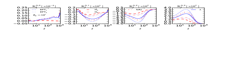
Figure 3: The kurtosis spectra $K^{A,i}_{\ell}$ defined in Eq.(4.28) for smoothing angular scale $\theta_{0}=10^{\prime}$ and $\ell_{max}=10^{3}$. From left they correspond to $K^{A,1}_{\ell}$ through to $K^{A,4}_{\ell}$. In each panel the base GR+$\Lambda$CDM model is shown along with five other modified gravity theories. The two effective field theory models are depicted by dashed line. The thick dotted lines correspond to the EFT₁ and the thin dotted lines correspond to EFT₂ respectively. The two dashed lines correspond to the Hořava models. The thick (thin) solid lines correspond to H₂(H₃). The doted lines correspond to the $f(R)$ model (see text for the description of these models). We haven’t included the $\sigma_{0}(\theta_{0})$ and $\sigma_{1}(\theta_{0})$ dependent normalisations in these plots to isolate the effect of MG theories on trispectrum.

These results are based on the following properties of the spherical harmonics:

$$\int\nabla_{i}Y_{\ell_{1}m_{1}}({\hat{\Omega}})\nabla^{i}Y_{\ell_{2}m_{2}}({\hat{\Omega}})Y_{LM}({\hat{\Omega}})d{\hat{\Omega}}={1\over 2}({\Pi}_{\ell_{1}}+{\Pi}_{\ell_{2}}-{\Pi}_{L})I_{\ell_{1}\ell_{2}L}\left(\begin{array}[]{ c c c }\ell_{1}&\ell_{2}&L\\ m_{1}&m_{2}&M\end{array}\right)$$ (4.22)

$$\nabla^{2}Y_{\ell m}({\hat{\Omega}})=-\Pi_{\ell}Y_{\ell m}({\hat{\Omega}})$$ (4.23)

Table 1: Survey Parameters [69]

Mission	Frequency (GHz)	Sensitivity ($\mu$K-arcmin)	$f_{\rm sky}$	FWHM
COrE+	145	$5.0$	70%	5.8′
ACTPol	150	$9.8$	50%	1.3′
Planck	143	$44.0$	50%	7.3′

Following the prescriptions in ref.[68] and ref.[70], the four generalised kurtosis $K^{(i)}$, which are one-point statistics, the concept of two-to-two $K^{A,i}_{\ell}$ and three-to-one $K^{B,i}_{\ell}$ kurt-spectra can now be introduced in terms of the generalised tri-spectra $T^{(i)}$ as follows:

$$K^{A,i}_{\ell}=\sum_{\ell_{i}}[T^{(i)}]^{\ell_{1}\ell_{2}}_{\ell_{3}\ell_{4}}(\ell)J_{\ell_{1}\ell_{2}\ell}J_{\ell_{3}\ell_{4}\ell};$$ (4.28)

$$K^{B,i}_{\ell}=\sum_{\ell_{i}}\sum_{L}[T^{(i)}]^{\ell_{1}\ell_{2}}_{\ell_{3}\ell}(L)J_{\ell_{1}\ell_{2}L}J_{L\ell_{3}\ell};$$ (4.29)

$$J_{\ell_{1}\ell_{2}\ell_{3}}={1\over\Xi_{\ell_{3}}}I_{\ell_{1}\ell_{2}\ell_{3}}.$$ (4.30)

These estimators generalises the optimized version of $K^{A,0}_{\ell}$ that has already been used in ref.[18] to constrain the projected mass exploiting the fact that the estimators $K^{A,0}_{\ell}$ and its higher order analogues are directly proportional to the lensing power-spectrum ${\cal C}_{\ell}^{\phi\phi}$.

The main advantage of using two-point estimators such as $K^{A,i}_{\ell}$ and $K^{B,i}_{\ell}$ is in the additional information contained in the shape of these spectra, which is useful in differentiating them from other secondary contributions e.g. kSZ.

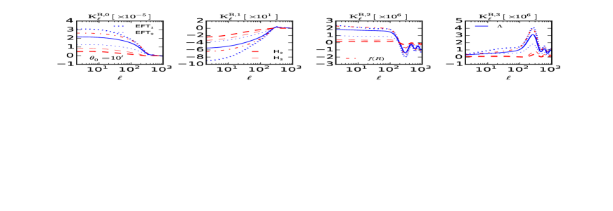
Figure 4: Same as previous figure but for the power-spectra $K^{B,i}_{\ell}$ as defined in Eq.(4.29).

The one-point statistics which are used as an input in Eq.(4.13) and Eq.(4.14) to construct the MFs, can be computed from their two-point counterparts:

$$K^{(i)}\equiv{1\over 4\pi}\sum_{\ell}\Xi_{\ell}\,K^{A,i}_{\ell}={1\over 4\pi}\sum_{\ell}\Xi_{\ell}\,K^{B,i}_{\ell}.$$ (4.31)

The physical meaning of these kurt-spectra can be understood more easily in the harmonic domain. Each individual mode of the trispectrum is characterized by a specific choice of set of modes ${\ell_{i}}$ that defines it. These modes each constitute the sides of a quadrilateral whose diagonal is specified by the harmonics $\ell$. The kurt-spectra $K_{\ell}^{A,i}$ considered here take contributions from all possible configurations of the quadrangle representing trispectrum while keeping its diagonal $\ell$ fixed. The kurt-spectra $K_{\ell}^{B,i}$ on the other hand represent the sum over all possible configurations of the quadrangle while keeping one of its side $\ell$ fixed.

The estimation of the kurt-spectra from real data is relatively easy and follows the same methodology as that of the skew-spectra. The first of these kurt-spectra $K^{(0)}$ is extracted by cross-correlating the squared field $[\Theta^{2}({\hat{\Omega}})]$ with itself. The spectra $K^{(1)}$ is constructed by cross-correlating $[\Theta^{2}({\hat{\Omega}})]$ against $[\Theta({\hat{\Omega}})\nabla^{2}\Theta({\hat{\Omega}})]$. The other two kurt-spectra can likewise be constructed. In each such construction a scalar map from a product field is generated before it is cross-correlated with another such map. The explicit expressions for the estimators $\hat{K}^{A,i}_{\ell}$ are as follows:

$$\hat{K}^{A,0}_{\ell}=A_{0}\,\hat{K}^{\Theta^{2},\Theta^{2}}_{\ell};\quad\hat{K}^{A,1}_{\ell}=A_{1}\,\hat{K}^{\Theta^{2},\Theta\nabla^{2}\Theta}_{\ell}$$ (4.32)

$$\hat{K}^{A,2}_{\ell}=A_{2}\,(2K_{\ell}^{\Theta\nabla^{2}\Theta,\nabla\Theta\cdot\nabla\Theta}+K_{\ell}^{\nabla\Theta\cdot\nabla\Theta,\nabla\Theta\cdot\nabla\Theta});\quad\hat{K}^{A,3}_{\ell}=A_{3}\,K^{\nabla\Theta\cdot\nabla\Theta,\nabla\Theta\cdot\nabla\Theta}_{\ell};$$ (4.33)

$$A_{0}={\sigma_{0}^{-6}};\quad A_{1}={\sigma_{0}^{-4}\sigma_{1}^{-2}};\quad A_{2}=A_{3}={\sigma_{0}^{-2}\sigma_{1}^{-4}}.$$ (4.34)

For current-generation surveys with small sky coverage, the correlation functions associated with the kurt-spectra may have some practical advantages. These are

$$K^{A,i}_{12}[\theta]\equiv{1\over 4\pi}\sum_{\ell}\Xi_{\ell}P_{\ell}(\cos\theta)\,K^{A,i}_{\ell}\;$$ (4.35)

$$K^{B,i}_{12}[\theta]\equiv{1\over 4\pi}\sum_{\ell}\Xi_{\ell}P_{\ell}(\cos\theta)\,K^{B,i}_{\ell}.$$ (4.36)

Here $P_{\ell}$ is a Legendre polynomial of order $\ell$. These two-point correlation functions (also known as cumulant correlators) are defined on the surface of the sphere between two line-of-sight directions separated by an angle $\theta$. For the special case of $\theta=0$ they both collapse to the same one-point cumulants defined in Eq.(4.31). However, in real space, correlation functions at two different angular scales are highly correlated, thus making error-analysis much more involved, even for all-sky coverage.

Two of the four three-to-one kurt-spectra $K_{\ell}^{B,2}$ and $K_{\ell}^{B,3}$ cannot be constructed using (cubic) combinations of scalar fields, as they involve gradients $\nabla\Theta$, and their co-ordinate independent constructions involve spinorial harmonics. From the point of view of construction of MFs $K_{\ell}^{A,i}$ and $K_{\ell}^{B,i}$ carry equivalent information. Also, as the spectra $K_{\ell}^{A,i}$ are not expressible as normalized lensing power spectrum ${\cal C}_{\ell}^{\phi\phi}$, they are less appealing for numerical implementation.

5 Estimators, Mask, Noise and Covariances

We have so far derived results for an ideal noise-free all-sky survey. In reality partial sky coverage and instrumental noise (possibly inhomogeneous) need to be dealt with. Partial sky coverage introduces mode-mode coupling in the harmonic domain in such a way that individual masked harmonics become linear combinations of all-sky harmonics. The coefficients for this linear transformation depend on specific choice of mask through its own harmonic coefficients. Based on the pseudo-${\cal C}_{\ell}$ (PCL) method devised in ref.[71] for power spectrum analysis, unbiased estimators for skew-spectra and kurt-spectra were later developed in ref.[39] and ref.[68] that can handle realistic data.

5.1 Estimators

Consider two generic fields $U({\hat{\Omega}})$ and $V({\hat{\Omega}})$ and denote their harmonic decompositions in the presence of a generic mask $w({\hat{\Omega}})$ as $\tilde{U}_{\ell m}$ and $\tilde{V}_{\ell m}$. The fields $U$ and $V$ may correspond to any of the fields we have considered above and the harmonics $\tilde{U}_{\ell m}$ and $\tilde{V}_{lm}$ will correspond to any of the harmonics listed in Eq.(4.32)- Eq.(4.34) i.e., $[\Theta^{2}]_{\ell m}$,   $[\nabla\Theta\cdot\nabla\Theta]_{\ell m}$ and $[\nabla^{2}\Theta]_{\ell m}$. The pseudo-harmonics of the masked fields are linear combinations of the ordinary harmonics:

$$\tilde{U}_{LM}=\int~{}d{\hat{\Omega}}~{}Y^{*}_{LM}({\hat{\Omega}})~{}[w({\hat{\Omega}})~{}U({\hat{\Omega}})];$$ (5.1)

$$\tilde{U}_{LM}=\sum_{\ell_{i}m_{i}}(-1)^{m}~{}I_{L\ell_{1}\ell_{2}}\left(\begin{array}[]{ c c c }\ell_{1}&\ell_{2}&L\\ m_{1}&m_{2}&-M\end{array}\right)w_{\ell_{1}m_{1}}U_{\ell_{2}m_{2}};$$ (5.4)

$$w_{lm}=\int~{}d{\hat{\Omega}}~{}Y^{*}_{\ell m}({\hat{\Omega}})~{}w({\hat{\Omega}}).$$ (5.5)

The construction of the pseudo kurt-spectra $\tilde{K}_{\ell}^{U,V}$ simply involves cross-correlating the relevant pseudo harmonics $\tilde{U}$ and $\tilde{V}$:

$$\tilde{K}_{L}^{U,V}(\theta_{b})={1\over\Xi_{L}}\Re\left[\sum_{m}\tilde{U}_{LM}\tilde{V}^{*}_{LM}\right];\quad\tilde{K}_{L}^{U,V}(\theta_{b})=\sum_{\ell^{\prime}}M_{L\ell^{\prime}}K_{\ell^{\prime}}^{U,V}(\theta_{b}).$$ (5.6)

The mixing matrix $M$ is a function of the power spectrum $w_{\ell}$ of the mask $w({\hat{\Omega}})$:

$$M_{LL^{\prime}}={1\over\Xi_{L}}\sum_{\ell}I^{2}_{LL^{\prime}\ell}|w_{\ell}|^{2};\quad\hat{K}_{L}^{U,V}(\theta_{b})=\sum_{\ell^{\prime}}[M^{-1}]_{L\ell^{\prime}}\tilde{K}_{\ell^{\prime}}^{U,V}(\theta_{b});$$ (5.7)

$$w_{\ell m}=\int w({\hat{\Omega}})Y^{*}_{\ell m}({\hat{\Omega}})d{\hat{\Omega}};\quad\quad w_{\ell}={1\over\Xi_{\ell}}\sum_{m}w_{\ell m}w^{*}_{\ell m}.$$ (5.8)

The estimator $\hat{K}_{L}^{U,V}(\theta_{b})$ constructed from pseudo-${\cal C}_{\ell}$s is unbiased as $\langle\hat{K}_{L}^{U,V}(\theta_{b})\rangle=K_{L}^{U,V}(\theta_{b})$. The scatter from the ensemble mean $\delta\hat{K}_{L}^{U,V}$ and its covariance $\langle\delta\hat{K}_{L}^{U,V}\delta\hat{K}_{L}^{U^{\prime},V^{\prime}}\rangle$ can be computed using the expressions given below:

$$\langle\hat{K}_{L}^{U,V}(\theta_{b})\rangle=K_{L}^{U,V}(\theta_{b});\quad\delta K_{L}^{U,V}(\theta_{b})=\hat{K}_{L}^{U,V}(\theta_{b})-\langle K_{L}^{U,V}(\theta_{b})\rangle;$$ (5.9)

$$\langle\delta\hat{K}_{L}^{U,V}(\theta_{b})\delta\hat{K}_{L^{\prime}}^{U,V}(\theta_{b})\rangle=\sum_{LL^{\prime}}M^{-1}_{L\ell}\langle\delta\tilde{K}_{\ell}^{U,V}(\theta_{b})\delta\tilde{K}_{\ell^{\prime}}^{U,V}(\theta_{b})\rangle M^{-1}_{\ell^{\prime}L^{\prime}};$$ (5.10)

$$\quad\quad\left\{U,V\right\}\in\left\{\Theta,\Theta^{2},(\nabla\Theta\cdot\nabla\Theta),\nabla^{2}\Theta\right\}.$$ (5.11)

For small sky-coverage the matrix $M_{\ell\ell^{\prime}}$ is singular and broad binning in the $\ell$ space may be required before the inversion.

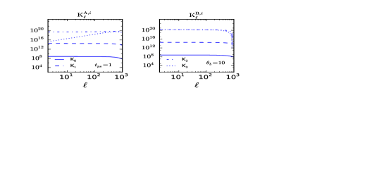
Figure 5: The four kurtosis-spectra $K^{A,i}_{\ell}$ as defined in Eq.(4.28) for unresolved point sources are shown in the left panel. Corresponding results for$K^{A,i}_{\ell}$ are defined in Eq.(4.29). The expression for the trispectrum of point-sources is given by Eq.(3.33). In each panel solid, dashed, dot-dashed and dotted lines correspond to $\rm K^{(0)}_{\ell}$, $\rm K^{(1)}_{\ell}$, $\rm K^{(2)}_{\ell}$ and $\rm K^{(3)}_{\ell}$ respectively. We assume $\theta_{0}=10^{\prime}$ and an all-sky coverage is assumed.

5.2 Error Covariance

The derivation of the covariance depends on a Gaussian approximation i.e. we ignore higher-order non-Gaussianity in the fields. ${\cal C}_{\ell}$ is the ordinary CMB power spectra it also includes the effect of instrumental noise and beam ${\cal C}_{\ell}^{t}(\theta_{b})={\cal C}^{S}_{\ell}b_{\ell}^{2}(\theta_{b})+n_{\ell}$. Such an approximation is suitable for noise-dominated surveys. Moreover, for a survey with homogeneous noise, we can write $n_{\ell}=\Omega_{p}\sigma_{N}^{2}$ where $\Omega_{p}$ is the pixel area and $\sigma_{N}$ is the noise r.m.s. The relations listed below, constructed using Wick’s theorem, will be useful in derivation of scatter for our estimators:

$$\langle\delta K_{L}^{U,V}(\theta_{b})\delta K_{L}^{U,V}(\theta_{b})\rangle_{c}={1\over\Xi_{L}}\left[K_{L}^{U,U}(\theta_{b})\;K_{L}^{V,V}(\theta_{b})+[K_{L}^{U,V}(\theta_{b})]^{2}\right];$$ (5.12)

$$\langle\delta K_{L}^{U_{1},V_{1}}(\theta_{b})\delta K_{L}^{U_{2},V_{2}}(\theta_{b})\rangle_{c}={1\over\Xi_{L}}\left[K_{L}^{U_{1},U_{2}}(\theta_{b})\;K_{L}^{V_{1},V_{2}}(\theta_{b})+K_{L}^{U_{1},V_{2}}(\theta_{b})\;K_{L}^{U_{2},V_{1}}(\theta_{b})\right].$$ (5.13)

The explicit expressions for the scatter and covariance that we will require are listed below:

$$\langle{\delta K^{A,0}_{L}\delta K^{A,0}_{L^{\prime}}}\rangle\equiv{\delta_{LL^{\prime}}}{2f_{\rm sky}^{-1}\over\Xi_{L}}A_{0}^{2}\Big{[}K_{L}^{{\Theta^{2},\Theta^{2}}}\Big{]}^{2};$$ (5.14)

$$\langle{\delta K^{A,1}_{L}\delta K^{A,1}_{L^{\prime}}}\rangle\equiv\delta_{LL^{\prime}}{f_{\rm sky}^{-1}\over\Xi_{L}}A_{1}^{2}\left[K_{L}^{\Theta^{2},\Theta^{2}}K_{L}^{\Theta\nabla^{2}\Theta,\Theta\nabla^{2}\Theta}+[K_{L}^{\Theta^{2},\Theta\nabla^{2}\Theta}]^{2}\right];$$ (5.15)

$$\langle\delta K^{A,2}_{L}\delta K^{A,2}_{L^{\prime}}\rangle_{c}=\delta_{LL^{\prime}}{f_{\rm sky}^{-1}\over\Xi_{L}}A_{2}^{2}\Big{[}4\,K_{L}^{\Theta\nabla^{2}\Theta,\Theta\nabla^{2}\Theta}K^{\nabla\Theta\nabla\Theta,\nabla\Theta\cdot\nabla\Theta}_{L}+4\,[K_{L}^{\Theta\nabla^{2}\Theta,\nabla\Theta\cdot\nabla\Theta}]^{2}{}$$

$$\hskip 85.35826pt+4\,K^{\Theta\nabla^{2}\Theta,\nabla\Theta\cdot\nabla\Theta}_{L}K_{L}^{\nabla\Theta\cdot\nabla\Theta,\nabla\Theta\cdot\nabla\Theta}+2\,[K_{L}^{\nabla\Theta\cdot\nabla\Theta,\nabla\Theta\cdot\nabla\Theta}]^{2}\Big{]};$$ (5.16)

$$\langle{\delta K^{A,3}_{L}\delta K^{A,3}_{L^{\prime}}}\rangle\equiv\delta_{LL^{\prime}}{2f_{\rm sky}^{-1}\over\Xi_{L}}{A_{3}^{2}}\Big{[}K_{L}^{\nabla\Theta\cdot\nabla\Theta,\nabla\Theta\cdot\nabla\Theta}\Big{]}^{2}.$$ (5.17)

Note that $\hat{K}_{\ell}^{A,2}$ gets contributions from two separate terms. Here $f_{sky}$ is the fraction of sky-coverage for the survey under consideration. Notice that unlike the skew-spectra and their generalisations introduced in ref.[43] kurtosis-spectra are not correlated in the limiting case of all-sky coverage. In this respect they are similar to the ordinary power spectrum. The individual expressions depends on the power spectrum:

$$K_{L}^{\Theta^{2},\Theta^{2}}={2}{1\over\Xi_{L}}\sum_{\{\ell_{i}\}=2}^{\ell_{max}}I^{2}_{\ell_{1}\ell_{2}L}{\cal C}^{t}_{\ell_{1}}{\cal C}^{t}_{\ell_{2}};\quad$$ (5.18)

$$K^{\Theta\nabla^{2}\Theta,\Theta\nabla^{2}\Theta}_{L}={1\over\Xi_{L}}\,{}\sum_{\{\ell_{i}\}=2}^{\ell_{max}}I^{2}_{\ell_{1}\ell_{2}L}\left[\Pi_{\ell_{1}}+\Pi_{\ell_{2}}\right]\,\Pi_{\ell_{2}}{\cal C}^{t}_{\ell_{1}}\,{\cal C}^{t}_{\ell_{2}}.$$ (5.19)

$$K^{\Theta^{2},\Theta\nabla^{2}\Theta}_{L}={-}{1\over\Xi_{L}}\sum_{\{\ell_{i}\}=2}^{\ell_{max}}I^{2}_{\ell_{1}\ell_{2}L}\left[\Pi_{\ell_{1}}+\Pi_{\ell_{2}}\right]{\cal C}^{t}_{\ell_{1}}{\cal C}^{t}_{\ell_{2}}$$ (5.20)

$$K_{L}^{\nabla\Theta\cdot\nabla\Theta,\nabla\Theta\cdot\nabla\Theta}={}{1\over 2}{1\over\Xi_{L}}\sum_{\{\ell_{i}\}=2}^{\ell_{max}}I^{2}_{\ell_{1}\ell_{2}L}\;[{\Pi}_{\ell_{1}}+{\Pi}_{\ell_{2}}-{\Pi_{L}}]^{2}\;{\cal C}^{t}_{\ell_{1}}{\cal C}^{t}_{\ell_{2}}$$ (5.21)

$$K_{L}^{\Theta\nabla^{2}\Theta,\nabla\Theta\cdot\nabla\Theta}=-{1\over\Xi_{L}}\sum_{\{\ell_{i}\}=2}^{\ell_{max}}{I^{2}_{\ell_{1}\ell_{2}L}}\;[{\Pi_{\ell_{1}}}+{\Pi}_{\ell_{2}}-{\Pi}_{L}]\;{\Pi_{\ell_{2}}}\;{\cal C}^{t}_{\ell_{1}}{\cal C}^{t}_{\ell_{2}};$$ (5.22)

$$K_{L}^{\Theta^{2},\nabla\Theta\cdot\nabla\Theta}={1\over\Xi_{L}}\sum_{\{\ell_{i}\}=2}^{\ell_{max}}{I^{2}_{\ell_{1}\ell_{2}L}}\;[{\Pi_{\ell_{1}}}+{\Pi}_{\ell_{2}}-{\Pi}_{L}]\;{\cal C}^{t}_{\ell_{1}}{\cal C}^{t}_{\ell_{2}},$$ (5.23)

where ${\cal C}^{t}_{\ell}$ is the total power spectrum, including contributions from detector noise. The expressions are symmetric under exchange of indices that are summed over i.e. $\ell_{1}$ and $\ell_{2}$ and we can restrict the summation to the upper triangular matrix $\sum^{\ell_{max}}_{\{\ell_{i}\}}=2\sum^{\ell_{max}}_{\ell_{1}=2}\sum^{\ell_{max}}_{\ell_{2}=\ell_{1}}$. We have included the expression in Eq.(5.23) will be required for the calculation of covariances. The signal-to-noise $[\rm S/\rm N]$ for individual modes for a given spectrum on the other hand can be expressed as:

$$[{\rm S/\rm N}]^{A,(i)}_{L}(\theta_{b})=\sqrt{\langle[K_{L}^{A,(i)}(\theta_{b})]^{2}\rangle/\langle[\delta K_{L}^{A,(i)}(\theta_{b})]^{2}\rangle}\quad\quad i\in\{0,1,2\}.$$ (5.24)

In our estimates of scatter we neglect contributions from terms describing higher-order non-Gaussianity such as the trispectrum. Thus, our results provide accurate results in the noise-dominated regime. For high sensitivity experiments Monte-Carlo simulation is the only way to evaluate the scatter. Also, we have assumed a uniform white noise, whereas in real experiments the noise will be non-uniform. Such complications can only be dealt with by running simulations. The parameters for a few ongoing and planned experiments are tabulated in Table 1, and the corresponding cumulative S/N for various estimators are listed in Table 2.

The estimators and the scatter are not independent. To compute the cross-correlation in scatter we will need the following expressions:

$$\langle\delta K^{A,0}_{L}\delta K^{A,1}_{L^{\prime}}\rangle_{c}\equiv\delta_{LL^{\prime}}{2{f^{-1}_{\rm sky}}\over\Xi_{L}}A_{0}A_{1}\left[K_{L}^{\Theta^{2},\Theta^{2}}K_{L}^{\Theta^{2},\Theta\nabla^{2}\Theta}\right];$$ (5.25)

$$\langle\delta K^{A,0}_{L}\delta K^{A,2}_{L^{\prime}}\rangle_{c}\equiv\delta_{LL^{\prime}}{2{f^{-1}_{\rm sky}}\over\Xi_{L}}A_{0}A_{2}\left[2K_{L}^{\Theta^{2},\Theta\nabla^{2}\Theta}K_{L}^{\Theta^{2},\nabla\Theta\cdot\nabla\Theta}+[K_{L}^{\Theta^{2},\nabla\Theta\cdot\nabla\Theta}]^{2}\right];$$ (5.26)

$$\langle\delta K^{A,0}_{L}\delta K^{A,3}_{L^{\prime}}\rangle_{c}\equiv\delta_{LL^{\prime}}{2{f^{-1}_{\rm sky}}\over\Xi_{L}}\;A_{0}A_{3}\left[K_{L}^{\Theta^{2},\nabla\Theta\cdot\nabla\Theta}\right]^{2};$$ (5.27)

$$\langle\delta K_{L}^{A,1}\delta K_{L^{\prime}}^{A,2}\rangle_{c}=\delta_{LL^{\prime}}{{f^{-1}_{\rm sky}}\over\Xi_{L}}\;A_{1}A_{2}\Big{[}2\,K_{L}^{\Theta^{2},\nabla\Theta\cdot\nabla\Theta}K_{L}^{\Theta\nabla^{2}\Theta,\Theta\nabla^{2}\Theta}{}$$

$$\hskip 56.9055pt+2\,K_{L}^{\Theta\nabla^{2}\Theta,\nabla\Theta\cdot\nabla\Theta}\,K_{L}^{\Theta^{2},\Theta\nabla^{2}\Theta}+K^{\Theta^{2},\nabla\Theta\cdot\nabla\Theta}_{L}K^{\Theta\nabla^{2}\Theta,\nabla\Theta\cdot\nabla\Theta}_{L}\Big{]};$$ (5.28)

$$\langle\delta K_{L}^{A,1}\delta K_{L^{\prime}}^{A,3}\rangle_{c}=\delta_{LL^{\prime}}{2{f^{-1}_{\rm sky}}\over\Xi_{L}}A_{1}A_{3}\left[K_{L}^{\Theta^{2},\nabla\Theta\cdot\nabla\Theta}K_{L}^{\Theta\nabla^{2}\Theta,\nabla\Theta\cdot\nabla\Theta}\right];$$ (5.29)

$$\langle\delta K_{L}^{A,2}\delta K_{L^{\prime}}^{A,3}\rangle_{c}\equiv\delta_{LL^{\prime}}{2{f^{-1}_{\rm sky}}\over\Xi_{L}}A_{2}A_{3}\Big{[}2K^{\Theta\nabla^{2}\Theta,\nabla\Theta\cdot\nabla\Theta}_{L}K^{\nabla\Theta\cdot\nabla\Theta,\nabla\Theta\cdot\nabla\Theta}_{L}{}$$

$$\hskip 142.26378pt+[K^{\nabla\Theta\cdot\nabla\Theta,\nabla\Theta\cdot\nabla\Theta}_{L}]^{2}\Big{]}.$$ (5.30)

The terms that appear in Eq.(5.25)-Eq.(5.30) can all be expressed in terms of quantities defined in Eq.(5.18)-Eq.(5.23). Notice that different harmonic modes of different estimators are uncorrelated in the all-sky limit. These expressions are used to compute the cross-correlation coefficient among various spectra which are defined below:

$$r^{ij}_{L}(\theta_{b})=\langle\delta K_{L}^{A,(i)}(\theta_{b})\delta K_{L}^{A,(j)}(\theta_{b})\rangle/\sqrt{\langle[\delta K_{L}^{A,(i)}(\theta_{b})]^{2}\rangle\langle[\delta K_{L}^{A,(j)}(\theta_{b})]^{2}\rangle};i,j\in\{0,1,2\}.$$ (5.31)

Throughout we have ignored mode-mode coupling. The coefficients of cross-correlation $r_{ij}$ are independent of the sky-coverage $f_{\rm sky}$ and normalisation coefficients $A_{i}$. Cross-correlation of generalised spectra $K^{A,i}_{\ell}$ and $K^{B,i}_{\ell}$ defined in Eq.(4.28)-Eq.(4.29) will vanish in the Gasussian limit as they will involve odd-order leading terms.

Notice that in our computation of error estimates we have ignored the error in the power spectrum ${\cal C}_{\ell}$, and assumed that the variances $\sigma_{0}^{2}$ and $\sigma_{1}^{2}$ are known exactly.

5.3 Computation of $\chi^{2}$

The departure between General Relativity (GR) and a modified gravity (MG) model, from various two-to-two estimators, can be quantified by:

$$\chi^{2}_{\phi\phi}=\sum_{ij}\sum_{\ell\ell^{\prime}}\delta{\cal C}^{\phi\phi,(i)}_{\ell}\;{\mathbb{C}}^{\phi\phi}_{ij,\ell\ell^{\prime}}\;\delta{\cal C}^{\phi\phi,(j)}_{\ell^{\prime}};\quad\quad{\delta{\cal C}}^{\phi\phi,(i)}_{\ell}={\cal C}^{\phi\phi,(i)}_{\ell}|_{\rm MG}-{\cal C}^{\phi\phi,(i)}_{\ell}|_{\rm GR}$$ (5.32)

We notice from Eq.(A.12)-Eq.(A.15) that we can construct an estimator for ${\delta{\cal C}}^{\phi\phi,(i)}_{\ell}$ from each $K^{A,(i)}_{\ell}$:

$${{\cal C}}^{\phi\phi,(i)}_{\ell}=[N^{(i)}_{\ell}]^{-1}K^{A,(i)}_{\ell};\quad{\mathbb{C}}^{\phi\phi}_{ij,\ell\ell^{\prime}}=[N^{(i)}_{\ell}]^{-1}[N^{(j)}_{\ell^{\prime}}]^{-1}\langle{\delta{K}}^{A,(i)}_{\ell}{\delta{K}}^{A,(j)}_{\ell^{\prime}}\rangle$$ (5.33)

Using these relations we can directly evaluate the $\chi^{2}$ using the covariance of $K^{A,(i)}_{\ell}$ (which we will denote as ${\mathbb{C}}^{A}_{ij,\ell\ell^{\prime}}$) presented in Eq.(5.14)-Eq.(5.17) and Eq.(5.25)-Eq.(5.30). :

$$\chi^{2}_{\phi\phi}=\sum_{ij}\sum_{\ell}\delta{K}^{A,i}_{\ell}\;[{\mathbb{C}}^{A}]^{-1}_{ij,\ell\ell}\;\delta{K}^{A,j}_{\ell^{\prime}};$$ (5.34)

$${\mathbb{C}}^{A}_{ij,\ell\ell}=\langle{\delta K}^{A,i}_{\ell}{\delta K}^{A,i}_{\ell}\rangle_{c};\quad{\delta{K}}^{A,i}_{\ell}={K}^{A,i}_{\ell}|_{\rm MG}-{K}^{A,i}_{\ell}|_{\rm GR}$$ (5.35)

We have used the fact that ${\mathbb{C}}^{A,i}$ is diagonal for an all-sky experiment. We will specialise this expression for $K^{A,3}_{\ell}$ as the (S/N) is considerably higher for this estimator and the other estimators have significant correlation with $K^{A,3}_{\ell}$.

6 Results and Discussion

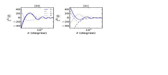
Figure 6: The correlation functions $\xi^{{\rm A},i}(\theta)$ (left-panel) and $\xi^{{\rm B},i}(\theta)$ (right-panel) defined respectively in Eq.(4.35) and Eq.(4.36) are shown as a function of $\theta_{12}$. A $\Lambda$CDM cosmology and GR is assumed. The solid, dashed, dot-dashed and dotted lines in left panel correspond to $\rm(A,0)\times 10^{-5}$, $\rm(A,1)\times 10^{1}$, $\rm(A,2)\times 10^{7}$ and $\rm(A,3)\times 10^{7}$ respectively. In the right panel they correspond to $\rm(B,0)\times 10^{-5}$, $\rm(B,1)\times 10^{1}$, $\rm(B,2)\times 10^{7}$ and $\rm(B,3)\times 10^{7}$. We have assumed the smoothing angular scale as $\theta_{0}=10^{\prime}$ and $\ell_{max}=10^{3}$.

Table 2: Cumulative ${\rm[S/N]}/f_{\rm sky}$ for various surveys

	K${}^{A,3}_{\ell}$	K${}^{A,2}_{\ell}$	K${}^{A,1}_{\ell}$	K${}^{A,0}_{\ell}$
ACTPol	1400	570	6.0	1.0
COrE+	2300	720	10.0	3.0
Planck	4.0	2.0	$8\times 10^{-2}$	$2\times 10^{-2}$

Table 3: ACTPol $\chi$ for various models

	H2	H3	Q	EFT1	EFT2	B0
K3	65	57	17	20	30	18
$\rm K_{2}$	1.5	1.0	3.9	5.0	7.0	4.0
$\rm K_{1}$	0.15	0.15	0.04	0.02	0.06	0.05
$\rm K_{0}$	0.04	0.04	0.01	0.006	0.02	0.01

Table 4: COrE⁺ $\chi$ for various models

	H2	H3	Q	EFT1	EFT2	B0
K3	94	87	25	26	43	30
$\rm K_{2}$	17	15	4.3	5.3	7.8	4.8
$\rm K_{1}$	0.4	0.4	0.1	0.05	0.18	0.13
$\rm K_{0}$	0.16	0.16	0.04	0.02	0.07	0.05

Table 5: Planck $\chi$ for various models

	H2	H3	Q	EFT1	EFT2	B0
K3	1.7	1.5	0.4	0.5	0.8	0.5
$\rm K_{2}$	.40	.36	0.1	0.01	0.19	0.1
$\rm K_{1}$	0.02	0.02	0.006	0.004	0.01	0.008
$\rm K_{0}$	0.008	0.008	0.002	0.001	0.003	0.003

1. The kurt-spectra we have defined depend on the lensing power spectra and the CMB temperature power spectra. In Fig.1 we show the $\cal C^{\phi\phi}_{\ell}$ as a function of $\ell$ for various MG theories. In Fig.2 the low-mulipole sector of the temperature power-spectrum ${\cal C}_{\ell}$ is shown.

2. The two-to-two and three-to-one estimators: The two-to-two and three estimators for various theories of gravity are shown in Fig.3 and Fig.4. The expressions in Eq.(4.28) and Eq.(4.29) define these two spectra. In our construction of these we have used the approximation $\rm T=P$, see e.g. Eq.(3.22), thereby ignoring the terms that involve computation of $6j$ coefficients. This approximation is commonly used in the literature and produces results which are reasonably accurate [63, 18]. This simplified our analytical results. Use of this approximation makes all two-to-two estimators directly proportional to the lensing potential power-spectra ${\cal C}^{\phi\phi}_{\ell}$. The normalisation coefficients depend on the harmonics $\ell$ and can be computed once the background cosmology is known. For the two-to-two spectra the individual $\ell$ modes are uncorrelated for all-sky surveys, which makes computation of statistics such as the $\chi^{2}$ statistic rather trivial. It depends only on the fiducial temperature power spectra. The two-to-two kurt-spectra for the unresolved point sources can be constructed equally easily. The correlation functions that we can define from these spectra Eq.(4.35) and Eq.(4.36) are shown in Fig.6. To compute the correlation functions we have included harmonics up to $\ell_{max}=10^{3}$ and a FWHM of $\theta_{0}=10^{\prime}$.

   The three-to-one spectra defined in Eq.(A.18)-Eq.(A.21) on the other hand depend on the lensing spectra through a convolution, which makes their interpretation complicated. Indeed, unlike the two-to-two estimators, the error-covariance of three-to-one spectra includes off-diagonal terms, even in the absence of any mask or non-uniform noise. In fact, it can be shown that all higher-order spectra at even order which are constructed by cross-correlating same combination of fields will have diagonal covariance matrix e.g. the ordinary power spectra which is one-to-one. At sixth order, the three-to-three spectra share the property of the two-to-two spectra, in having diagonal covariance, with an $f_{\rm sky}$ prescription being used to take into account the mode-mode coupling. However, any other spectra such as the two-to-one skew-spectra or the three-to-one kurt spectra will exhibit off-diagonal elements, as they are not an auto-spectra of a quadratic $[\Theta^{2}]$ or cubic $[\Theta^{3}]$ combination.

   The implementation of three-to-one spectra is also difficult, since to decompose a cubic combination involving partial derivatives we have to use spinorial spherical harmonics.

3. The variance and cross-correlation: The variance of the estimators is presented in Fig.7. Of all the estimators we have studied the estimator $K^{A,3}_{\ell}$ has the maximum (S/N) followed by $K^{A,2}_{\ell}$. The (S/N) is typically high for $\ell=10^{2}-10^{3}$. The other two estimators lack the (S/N) needed to be useful. The expressions in Eq.(5.14)-Eq.(5.17) gives the expressions for the variance in these estimators. This is in qualitative agreement with ref.[25] where the ordinary kurtosis parameter was studied and was found to lack the value of (S/N) needed for detection even in a cosmic variance dominated survey. Eq.(5.25)-Eq.(5.30) defines the cross-correlations. To compute the scatter and correlation of our estimators are defined in terms of quantities defined in the expressions in Eq.(5.18)-Eq.(5.23). Computations of these expressions are based on the assumption that the underlying CMB harmonics are Gaussian. All higher order non-Gaussianities are ignored, and we have assumed that the noise is independent of pixel position to simplify our analytical results. It is indeed possible to define more sophisticated estimators that work directly with the Wiener-filtered harmonics [72] to improve the (S/N). For more accurate estimates of (S/N) it is possible to employ simulation chain using software such as the Lenspix that can handle inhomogeneous noise. The power-spectra ${\cal C}^{\phi\phi}_{\ell}$ we have used are based on linear theory. Numerical simulations and non-linear modelling have been used to compute the nonlinear corrections to ${\cal C}^{\phi\phi}_{\ell}$ [73]. Such calculations are lacking at present for many of the MG theories we have considered. Construction of our estimators do not depend on the shape of $\cal C^{\phi\phi}_{\ell}$ and inclusion of non-linearity is unlikely to change the qualitative results presented here.

4. MG theories and $\chi^{2}$: In Table 2 we find that surveys such as ACTPol or CoRE⁺ should be able to detect the lensing of the CMB in temperature maps with extremely high S/N. However, a few comments are in order, since we have used a simple model for covariance. In practice, we will have to deal with inhomogeneous noise, the connected part of the covariance matrix and any residuals from component separation. The $\chi^{2}_{\phi\phi}$ defined in Eq.(5.34)-Eq.(5.35) for various survey configuration are displayed in Tables 3,4,5.

   However, even if we consider our estimates as no more than an order magnitude estimate they still are impressive. The models that we have considered are already rejected by other observational data e.g. the $f(R)$ models. For reference, we note that the designer $f(R)$ gravity, the constraint on its Compton wavelength parameter ($B_{0}$) from the latest Planck-2015 data are presented in ref. [12], $B_{0}<0.12~{}(0.04)$ at $95\%$ C.L. by using the compilation of temperature and low multipole polarization data, (the number in the parentheses is the one adding CMB lensing data).

   Our study suggests that the future lensing data will further tighten the constraints and render them comparable to constraints from the local tracers of large-scale structure of the Universe such as the weak-lensing surveys or galaxy surveys. Also, we have focussed on MG theories but similar results are expected for neutrino mass hierarchy (Munshi et al. in prep.).

   Inclusion of polarization data will further improve the result. In addition to the surveys we have focussed there are many surveys that are being planned such as the EBEX, Simons Array survey or the LiteBird surveys.

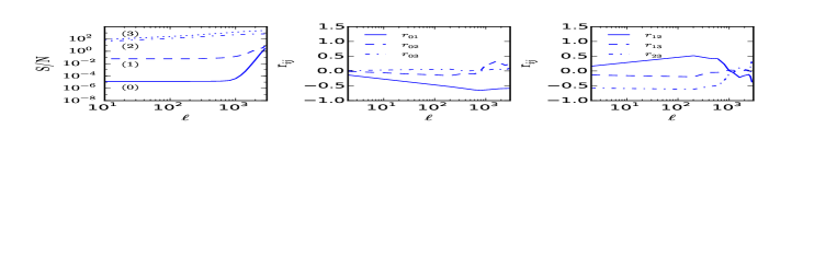
Figure 7: The cumulative sum of the $\rm S/N$ is plotted as a function of $\ell$. The solid, dashed, dot-dashed and dotted lines correspond to $K^{(0)}_{\ell}$, $K^{(1)}_{\ell}$, $K^{(2)}_{\ell}$ and $K^{(3)}_{\ell}$. The $\rm S/N$ is defined in Eq.(5.24). The individual modes of a given kurt-spectra are uncorrelated. However, for a given $\ell$ the estimates of various kurt-spctra are correlated. The correlation coefficients defined in Eq.(5.31) are plotted as a function of $\ell$ in middle and right panel. The middle panel shows $r_{01}$ (solid-lines), $r_{02}$ (dashed-lines) and $r_{03}$ (dot-dashed lines). The right panel shows $r_{23}$ (solid-lines), $r_{24}$ (dashed-lines) and $r_{34}$ (dot-dashed lines) respectively. We have taken $\ell_{max}=3000$ and the noise and beam correspond to that of the ACTPol survey. (see text for more details).

7 Conclusions and Outlook

In this paper, we have studied how lensing of the CMB can change the topological properties of temperature and polarization maps by using morphological descriptors such as the Minkowski Functionals. A perturbative expansion links MFs with the multispectra of the lensed maps. Recent studies have shown how statistics such as the skew-spectra [40] can be valuable in reconstructing MFs of frequency cleaned maps at the level of lensing-secondary bispectrum, frequency-cleaned tSZ maps [47], maps from weak lensing surveys [48]. The primary aim of this study was to extend these results to include the lensing induced trispectrum in the analysis. We have used the kurt-spectra introduced in ref.[70] for this purpose.

The shape of the kurt-spectra is a natural diagnostics in distinguishing different sources of non-Gaussianity. We construct a set of four kurt-spectra based estimators that are directly proportional to the power spectrum ${\cal C}_{\ell}^{\phi\phi}$ of the projected lensing-potential $\phi$, which is a sensitive probe of the neutrino mass hierarchy and DE equation of state, and thus provide a set of sub-optimal estimators for the reconstruction of lensing potential power spectrum. We have used them to study various MG theories.

1. Component Separation using non-Gaussianity: kurt-Spectra and topology of reionization: It was pointed out in ref.[46] that lensing (a gravitational secondary) and kSZ (a scattering secondary) share many interesting properties. Both of these secondaries lack any frequency information that can help them to separate from primary CMB. These secondaries on the other hand are non-Gaussian and this information can be used to separate them. The kurtosis is the leading order non-Gaussianity for both kSZ and lensing of CMB as all odd order contributions vanish for both these secondaries [74]. While lensing is an important probe of gravitational physics, kSZ is an important probe of reionization history of the Universe. Reionization can in principle be inhomogeneous. In ref.[46] only the three-to-one estimator was used and the non-Gaussian contribution to lensing were ignored. The systematic analysis we have performed for both three-to-one and two-to-two estimators show that simultaneous analysis of these two effects is possible, and using the two set of estimators can separate the contributions without imposing any further constraints. The topological estimators which we have developed here Eq.(4.28)-Eq.(4.29) or its real-space analogs Eq.(4.35)-Eq.(4.36) can be employed to understand the topology of inhomogeneous reionization using data from next generation of experiments (Munshi et al. in prep. 2016). We provide explicit expressions for the error-analysis of these spectra which are completely generic and can also be used for kSZ [74].

2. Polarization and separation of gradient and curl modes: In future the measurement of ${\cal C}^{\phi\phi}_{\ell}$ will be able to provide much tighter constraints on cosmological parameters using not just the temperature but polarization data. In addition to provide tighter constraints on neutrino masses, DE models and MG theories the ultimate goal of CMB experiments will be to detect the primordial gravity wave signals through the measurement of B-polarization. The signal however is confused with lensing effect. The lensing effect converts the dominant E-polarization to $B$-modes. The estimators designed here can be used to separate the signal from primordial gravitational waves and lensing of E-modes. We incorporated only the gradient modes in our results. However the curl mode that can be useful also for computing contribution from gravitational wave, cosmic strings or primordial magnetic field [75] can easily be included in our results. Generalisation of the results discussed here to polarization will be presented elsewhere.

3. Separation of $f_{\rm NL}$ and $g_{\rm NL}$: The optimized versions of two-to-two and three-to-one estimators have been used to probe primordial non-Gaussianity beyond the lowest order i.e. to separate contributions from $\tau_{\rm NL}$ and $g_{\rm NL}$ [18]. Although current experimental results are consistent with null detection of non-Gaussianiy, consistency check from future experiments can be performed using the estimators defined here beyond the lowest order.

   The estimators can be generalised to the study of primordial trispectra using CMB spectral distortions [76].

The pseudo-${\cal C}_{\ell}$ formalism discussed above is sub-optimal but extremely fast and its error covariance can be computed analytically as we have shown. These estimators are sub-optimal. However, in near future large fraction of the sky will be covered by experiments which will have very low detector noise and small FWHM, thus optimality of estimators may not be a crucial requirement in the future.

8 Acknowledgements

DM and PC acknowledge support from the Science and Technology Facilities Council (grant number ST/L000652/1). DM would like to thank Julien Peloton, Donough Regan, Antony Lewis and Joseph Smidt for useful discussions. DM also acknowledges Patrick Valageas and Geraint Pratten for related collaborations. BH is partially supported by the Programa Beatriu de Pinós and Dutch Foundation for Fundamental Research on Matter (FOM).

Appendix A Explicit Expressions for the Kurtosis-Spectra

A.1 Computation of disjoint or Gaussian contribution

The Gaussian components of the estimators are as follows:

$${G}_{L}^{A,0}=A_{0}{\cal G}_{L}^{(a)};$$ (A.1)

$${G}_{L}^{A,1}=-A_{1}{\cal G}_{L}^{(b)};$$ (A.2)

$${G}_{L}^{A,2}=-A_{2}\left[{\Pi}^{2}_{L}\,{\cal G}_{L}^{(a)}-{\cal G}_{L}^{(c)}\right];$$ (A.3)

$$G_{L}^{A,3}=A_{3}\left[{{\Pi}_{L}}^{2}{\cal G}_{L}^{(a)}-2{{\Pi}_{L}}{\cal G}_{L}^{(b)}+{\cal G}_{L}^{(c)}\right];$$ (A.4)

$${\cal G}_{L}^{(a,b,c)}={1\over 2\pi}\sum_{\ell_{1}\ell_{2}}\;Z^{(a,b,c)}\;I^{2}_{\ell_{1}L\ell_{2}}{\cal C}_{\ell_{1}}{\cal C}_{\ell_{2}};$$ (A.5)

$$Z^{(a)}_{\ell_{1}\ell_{2}}=1;\quad Z^{(b)}_{\ell_{1}\ell_{2}}={\Pi}_{\ell_{1}}+{\Pi}_{\ell_{2}};\quad Z^{(c)}_{\ell_{1}\ell_{2}}=({\Pi}_{\ell_{1}}+{\Pi}_{\ell_{2}})^{2}.$$ (A.6)

The first term in each of these expressions denotes the monopole contribution $\ell=0$, and the second term corresponds to $\ell\neq 0$. Notice these expressions depend on the total power spectrum of both signal (beam-convolved) and noise (which is assumed Gaussian) i.e., ${\cal C}^{t}_{\ell}={\cal C}_{\ell}^{S}b_{\ell}^{2}(\theta_{0})+n_{\ell}$. The corresponding three-to-one estimators in the Gaussian limit are

$$G^{B,0}_{L}=B_{0}\,S^{(00)}_{L}$$ (A.7)

$$G^{B,1}_{L}=2B_{1}\,S^{(01)}_{L}$$ (A.8)

$$G^{B,2}_{L}=B_{2}\,[S^{(20)}_{L}-S^{(02)}_{L}]$$ (A.9)

$$G^{B,3}_{L}=B_{3}\,[S^{[20]}_{L}+S^{[02]}_{L}-2S^{[11]}_{L}],$$ (A.10)

where we have introduced the quantities $S^{pq}_{\ell}$ to simplify the expressions:

$$S^{pq}_{L}={{\cal C}_{L}\over\Xi_{L}}\sum_{\ell_{1}\ell_{2}}{{\cal C}_{\ell_{1}}\over\Xi_{\ell_{2}}}\Pi^{p}_{L}(\Pi_{\ell_{1}}+\Pi_{L})^{q}{\cal C}_{\ell_{1}}I^{2}_{\ell_{1}L\ell_{2}}.$$ (A.11)

If we use the same normalisation as the two-to-two estimators we have $A_{i}=B_{i}$.

A.2 Lensing induced two-to-two Kurtosis-Spectra $K_{\ell}^{A,(i)}$

We will specialise the kurt-spectra we have derived in the text of the paper for the special case of lensing-induced non-Gaussianity. All of the two-to-two spectra or equivalently the $K_{\ell}^{A,i}$ estimators we have studied can be expressed as a product of the lensing power spectrum ${\cal C}_{\ell}^{\phi\phi}$, times an $\ell$-dependent normalisation:

$$K_{L}^{A,0}=A_{0}\,{\cal C}^{\phi\phi}_{L}{1\over\Xi^{2}_{L}}[{\cal E}_{L}^{(0)}]^{2};\quad$$ (A.12)

$$K_{L}^{A,1}=A_{1}\,{\cal C}^{\phi\phi}_{L}{1\over\Xi^{2}_{L}}{\cal E}_{L}^{(0)}\,{\cal E}_{L}^{(1)};$$ (A.13)

$$K_{L}^{A,2}=A_{2}\,{\cal C}^{\phi\phi}_{L}{1\over\Xi^{2}_{L}}\left[{\Pi^{2}_{L}}[{\cal E}_{L}^{(0)}]^{2}-[{\cal E}_{L}^{(1)}]^{2}\right];\quad$$ (A.14)

$$K_{L}^{A,3}=A_{3}\,{\cal C}^{\phi\phi}_{L}{1\over\Xi^{2}_{L}}\,[{\cal E}_{L}^{(1)}-{\Pi_{L}}{\cal E}_{L}^{(0)}]^{2}.$$ (A.15)

The factors ${\cal E}_{L}^{(0)}$ and ${\cal E}_{L}^{(1)}$ depend only on the power spectrum of the unlensed CMB sky ${\cal C}_{\ell}$ and are defined below :

$${\cal E}_{L}^{(0)}\equiv\sum_{\ell_{1}\ell_{2}}f_{\ell_{1}L\ell_{2}}I_{\ell_{1}L\ell_{2}};\quad{\cal E}^{(1)}_{L}\equiv\sum_{\ell_{1}\ell_{2}}(\Pi_{\ell_{1}}+\Pi_{\ell_{2}})f_{\ell_{1}L\ell_{2}}I_{\ell_{1}L\ell_{2}}.$$ (A.16)

For point sources we can use the expressions Eq.(A.12)-Eq.(A.15) by redefining the ${\cal E}$ matrices:

$${\cal E}_{L}^{{\rm ps},(0)}\equiv\sum_{\ell_{1}\ell_{2}}I^{2}_{\ell_{1}L\ell_{2}};\quad{\cal E}^{{\rm ps},(1)}_{L}\equiv\sum_{\ell_{1}\ell_{2}}(\Pi_{\ell_{1}}+\Pi_{\ell_{2}})I^{2}_{\ell_{1}L\ell_{2}}.$$ (A.17)

The normalisation coefficients $A_{i}$ will remain unchanged but the ${\cal C}^{\phi\phi}_{\ell}$ will have to be replaced with the amplitude for the unresolved point source trispectrum $t_{\rm ps}$ introduced in Eq.(3.33).

A.3 Lensing induced three-to-one Kurtosis-Spectra $K_{\ell}^{B,(i)}$

In this section we will compute the three-to-one term from lensing. The construction of the estimator follows exactly same procedure as for the two-to-two estimator. We list the expressions below :

$$K_{L}^{B,0}=A_{0}\,{1\over\Xi_{L}}\sum_{\ell}{{\cal C}_{\ell}^{\phi\phi}\over\Xi_{\ell}}{\cal D}^{(0)}_{\ell L}{\cal E}^{(0)}_{\ell};$$ (A.18)

$$K_{L}^{B,1}=A_{1}\,{1\over\Xi_{L}}\sum_{L}{{\cal C}_{\ell}^{\phi\phi}\over\Xi_{\ell}}\left[{\cal D}^{(1)}_{\ell L}{\cal E}^{(0)}_{\ell}+{\cal D}^{(0)}_{\ell L}{\cal E}^{(1)}_{\ell}\right];$$ (A.19)

$$K_{L}^{B,2}=A_{2}\,{1\over\Xi_{L}}\sum_{\ell}{{\cal C}_{\ell}^{\phi\phi}\over\Xi_{\ell}}\left[\Pi^{2}_{\ell}{\cal D}^{(0)}_{\ell L}{\cal E}^{(0)}_{\ell}-{\cal D}^{(1)}_{\ell L}{\cal E}^{(1)}_{\ell}\right];$$ (A.20)

$$K_{L}^{B,3}=A_{3}\,{1\over\Xi_{L}}\sum_{\ell}{{\cal C}_{\ell}^{\phi\phi}\over\Xi_{\ell}}\left[(\Pi_{\ell}{\cal D}^{(0)}_{\ell L}-{\cal D}^{(1)}_{\ell L})(\Pi_{\ell}{\cal E}^{(0)}_{\ell}-{\cal E}^{(1)}_{\ell})\right].$$ (A.21)

The amplitudes $A_{i}$ are same as the ones for the corresponding two-to-two spectra introduced before. We have introduced the following quantities to simplify our notation:

$${\cal D}^{(0)}_{\ell\,L}\equiv\sum_{\ell^{\prime}}f_{\ell^{\prime}L\ell}I_{\ell^{\prime}L\ell};\quad{\cal D}^{(1)}_{\ell\,L}\equiv\sum_{\ell^{\prime}}(\Pi_{\ell}+\Pi_{\ell^{\prime}})f_{\ell^{\prime}L\ell}I_{\ell^{\prime}L\ell}.$$ (A.22)

Note that the ${\cal D}$ matrices are not symmetric in their indices. The quantities ${\cal E}^{(0)}_{L}$ and ${\cal E}^{(1)}_{L}$ defined in Eq.(A.16) can now be expressed in terms of ${\cal D}^{(0)}_{\ell L}$ and ${\cal D}^{(1)}_{\ell L}$:

$${\cal E}^{(0)}_{L}\equiv\sum_{\ell}{\cal D}^{(0)}_{\ell L};\quad{\cal E}^{(1)}_{L}\equiv\sum_{\ell}{\cal D}^{(1)}_{\ell L}.$$ (A.23)

From Eq.(A.18)-Eq.(A.21), notice that the three-to-one estimator, unlike the two-to-two estimators, cannot be written in terms of the lensing power spectrum times an $\ell$-dependent normalisation factor. Instead, it involves a convolution, encapsulated in the ${\cal D}$ matrices. For point sources we have:

$${\cal D}^{{\rm ps},(0)}_{\ell L}\equiv\sum_{\ell^{\prime}}I^{2}_{\ell^{\prime}L\ell};\quad{\cal D}^{{\rm ps},(1)}_{\ell L}\equiv\sum_{\ell^{\prime}}(\Pi_{\ell}+\Pi_{\ell^{\prime}})I^{2}_{\ell^{\prime}L\ell}.$$ (A.24)

The covariances of the first two of these estimators can be computed using similar technique as before:

$$\langle\delta K^{B,1}_{\ell}\delta K^{B,1}_{\ell^{\prime}}\rangle=\delta_{\ell\ell^{\prime}}\;6{1\over\Sigma^{2}_{\ell}}{\cal C}_{\ell}{\cal Q}_{\ell}+{\cal C}_{\ell}{\cal C}_{\ell^{\prime}}{1\over\Xi_{\ell}}{1\over\Xi_{\ell^{\prime}}}{\cal R}_{\ell}{\cal R}_{\ell^{\prime}};$$ (A.25)

$$\langle\delta K^{B,2}_{\ell}\delta K^{B,2}_{\ell^{\prime}}\rangle=\delta_{\ell\ell^{\prime}}\;6{\Pi^{2}_{\ell}\over\Sigma^{2}_{\ell}}\;{\cal C}_{\ell}{\cal Q}_{\ell}+{\cal C}_{\ell}{\cal C}_{\ell^{\prime}}{{\Pi}_{\ell}\over\Xi_{\ell}}{{\Pi}_{\ell^{\prime}}\over\Xi_{\ell^{\prime}}}{\cal R}_{\ell}{\cal R}_{\ell^{\prime}}.$$ (A.26)

The new quantities we have introduced are

$${\cal Q}_{\ell}=\sum_{\ell_{i}=2}\sum_{L}{\cal C}_{\ell_{1}}{\cal C}_{\ell_{2}}{\cal C}_{\ell_{3}}I^{2}_{\ell_{1}\ell_{2}L}I^{2}_{L\ell_{3}\ell}$$ (A.27)

$${\cal R}_{\ell}=\sum_{\ell_{2}}\sum_{L}{\cal C}_{\ell_{2}}I^{2}_{L\ell_{2}\ell}.$$ (A.28)

We have assumed the absence of any parity-violating physics, and ignore the $L=0$, as discussed before. The results are valid for all-sky coverage. The two-to-two estimators and their three-to-one counterparts are decorrelated in the Gaussian limit as the leading order terms take contribution from odd-order multispectra.

Appendix B Recovery of the Generalised Kurtosis Parameters

The generalised kurtosis can be recovered using either the two-to-two or three-to-one kurt-spectra by using the Eq.(4.31), and are given by the following expressions:

$$K^{(0)}=\sum_{L}{{\cal C}^{\phi\phi}_{L}\over\Xi_{L}}{{\cal E}_{L}^{(0)}}^{2};$$ (B.1)

$$K^{(1)}=2\,\sum_{L}{{\cal C}^{\phi\phi}_{L}\over\Xi_{L}}{\cal E}_{L}^{(0)}{\cal E}_{L}^{(1)};$$ (B.2)

$$K^{(2)}=\sum_{L}{{\cal C}^{\phi\phi}_{L}\over\Xi_{L}}\left[\Pi^{2}_{L}\,{{\cal E}_{L}^{(0)}}^{2}-{{\cal E}_{L}^{(1)}}^{2}\right];$$ (B.3)

$$K^{(3)}=\sum_{L}{{\cal C}^{\phi\phi}_{L}\over\Xi_{L}}\left[\Pi_{L}\,{\cal E}_{L}^{(0)}-{{\cal E}_{L}^{(1)}}\right]^{2}.$$ (B.4)

The quantities ${\cal E}^{(0)}_{L}$ and ${\cal E}^{(1)}_{L}$ are given in Eq.(A.16). To compute corresponding estimates for the point sources we have to replace ${\cal C}^{\phi\phi}_{L}$ by the amplitude $t_{\rm ps}$ and ${\cal E}_{L}^{(i)}$ with their point-source analogues ${\cal E}_{L}^{\rm ps,(i)}$ defined in Eq.(A.17).

Appendix C Kurt-Spectra as Sub-Optimal Estimators for Lensing Reconstruction

The kurt-spectra $K_{\ell}^{A,i}$, introduced in this paper in Eq.(4.32)-Eq.(4.34), are constructed from a combination of cross-spectra such as $K_{\ell}^{\Theta^{2},\;\Theta^{2}}$, $K_{\ell}^{\Theta^{2},\Theta\nabla^{2}\Theta}$, or in general $K_{\ell}^{\Psi_{\alpha},\Psi_{\beta}}$, where $\Psi_{\alpha}$ and $\Psi_{\beta}$ are chosen form $\{\Theta^{2},\Theta\nabla^{2}\Theta,\nabla\Theta\cdot\nabla\Theta\}$. The multipole expansion of the derived temperature maps $\Psi_{\alpha}$ are a set of quadratic statistics that can be used as sub-optimal estimators for reconstruction of lensing potential $\phi$ as we will see below.

The harmonic coefficients of the lensing potential $\phi_{\ell m}$ in general can be expressed in terms of such quadratic combination $\Psi$ with a suitable $\ell$ normalization through a convolution which depends on the weight function $g_{\ell_{1}\ell_{2}\ell}$:

$$\hat{\phi}_{\ell m}={1\over\Psi_{\ell}}\hat{\Psi}_{\ell m};\quad\quad\Psi_{\ell}=\sum_{\ell_{1}\ell_{2}}g^{\psi}_{\ell_{1}\ell\ell_{2}}f_{\ell_{1}\ell_{2}\ell}.$$ (C.1)

$$\hat{\phi}_{\ell m}={1\over\Psi_{\ell}}\sum_{\ell_{1}m_{1}}\sum_{\ell_{2}m_{2}}(-1)^{m}g^{\Psi}_{\ell_{1}\ell\ell_{2}}\left(\begin{array}[]{ c c c }\ell_{1}&\ell_{2}&\ell\\ m_{1}&m_{2}&-m\end{array}\right)\hat{\Theta}_{\ell_{1}m_{1}}\hat{\Theta}_{\ell_{2}m_{2}}.$$ (C.4)

For a specific choice of $\Psi$ the resulting weights are listed below:

$$g_{\ell_{1}\ell_{2}\ell}^{\Theta^{2}}=I_{\ell_{1}\ell_{2}\ell};\quad g_{\ell_{1}\ell_{2}\ell}^{\Theta\nabla^{2}\Theta}=-\Pi_{\ell_{1}}I_{\ell_{1}\ell_{2}\ell};\quad g_{\ell_{1}\ell_{2}\ell}^{\nabla\Theta\cdot\nabla\Theta}={1\over 2}I_{\ell_{1}\ell_{2}\ell}\Lambda_{\ell_{1}\ell\ell_{2}}.$$ (C.5)

This result is completely generic and does not depend on a specific choice of the weighting function $g_{\ell_{1}\ell_{2}\ell}$, although we have approximated $T=P$. Additional terms will contribute to bias and can be removed for any practical application.

Reconstruction of individual harmonics $\phi_{lm}$ is expected to be noise-dominated so the reconstruction is typically carried out for the power-spectrum ${\cal C}_{l}^{\phi\phi}$ of the lensing potential $\phi$. Thus we can construct a series of estimator for ${\cal C}_{\ell}^{\phi\phi}$ using the two-to-two estimators.

$$\hat{\cal C}_{\ell}^{(\alpha,\beta),\phi\phi}={1\over\Psi_{\ell}^{(\alpha)}\Psi_{\ell}^{(\beta)}}\hat{K}_{\ell}^{(\alpha,\beta)}$$ (C.6)

The other set of estimators that we have studied i.e. $K_{l}^{B,(i)}$ involves a convolution of $C_{\ell}^{\phi\phi}$ and temperature power spectrum $\bar{\cal C}_{l}$. Though these estimators can not be used directly for reconstruction of ${\cal C}_{l}^{\phi}$ they can be used for cross-validation of results obtained using $K_{l}^{A,(i)}$.

For the optimal estimator presented in Ref.[64] the weight function $g_{\ell_{1}\ell_{2}\ell}$ takes the following form: $g_{\ell_{1}\ell_{2}L}=(f_{\ell_{1}\ell\ell_{2}}/\bar{\cal C}_{\ell_{1}}\bar{\cal C}_{\ell_{2}})$. Though primarily designed to analyse the morphological properties, they can also work as sub-optimal estimators for lensing reconstruction and are faster than their optimal counterpart, as they can be implemented using the pseudo-${\cal C}_{\ell}$ approach described in §5.

References

- [1] Planck Collaboration, The Scientific Programme of Planck , [astro-ph/0604069].
- [2] The COrE Collaboration COrE (Cosmic Origins Explorer) A White Paper , [arXiv/1102.2181].
- [3] Kermish Z. et al., Presented at SPIE Millimeter, Submillimeter, and Far-Infrared Detectors and Instrumentation for Astronomy VI, July 6, 2012. To be published in Proceedings of SPIE Volume 8452,
- [4] Niemack M.D. et. al. ACTPol: A polarization-sensitive receiver for the Atacama Cosmology Telescope [arXiv/1006.5049].
- [5] McMahon J., et al., 2009, American Institute of Physics Conference Series, 1185, 511
- [6] Knox L., Song Y.-S., 2002, PRL, 89, 011303 A limit on the detectability of the energy scale of inflation [astro-ph/0202286]
- [7] Seljuk U., Hirata C., 2004, PRD, 69, 043005 Analyzing weak lensing of the cosmic microwave background using the likelihood function [astro-ph/0202286]
- [8] Kaplinghat M., Knox L., Song Y.-S. 2003, PRL, 91,241301 Determining Neutrino Mass from the CMB Alone [astro-ph/0202286]
- [9] Lesgourgues J., Perotto L., Pastor S., Piat M., 2006, PRD, 73, 045021 Probing neutrino masses with CMB lensing extraction [astro-ph/0202286]
- [10] de Putter R., Zahn O., Linder E.V., 2009, PRD, 79, 065033 CMB Lensing Constraints on Neutrinos and Dark Energy [astro-ph/0202286]
- [11] Hu B., Liguori M., Bartolo N., Matarrese S., 2013, PRD, 88, no. 2, 024012 Future CMB ISW-Lensing bispectrum constraints on modified gravity in the Parameterized Post-Friedmann formalism [astro-ph/0202286]
- [12] Planck Collaboration, 2015, Planck 2015 results. XIV. Dark energy and modified gravity, [arXiv/1502.01590].
- [13] Lewis A., Challinor A., 2005, PRD, 71, 103010 Weak Gravitational Lensing of the CMB [astro-ph/0202286]
- [14] Hirata C.M., Ho S., Padmanabhan N., Seljak U., Bhacall N.A., 2008, PRD, 78, 043520
- [15] Smith K.M., Zahn O., Dore O., 2007, Phys. Rev. D, 76, 043510 Detection of Gravitational Lensing in the Cosmic Microwave Background [arXiv/0705.3980]
- [16] Das S., et al., 2011, PRL, 107, 021301 Detection of the Power Spectrum of Cosmic Microwave Background Lensing by the Atacama Cosmology Telescope [arXiv/1103.2124]
- [17] van Engelen A., et al., 2012, ApJ, 756, 142 A measurement of gravitational lensing of the microwave background using South Pole Telescope data [arXiv/1202.0546]
- [18] Smidt J., Cooray A., Amblard A., Joudaki S., Munshi D., Santos M. G., Serra, P., 2011, ApJL, 728, 1 A Constraint On the Integrated Mass Power Spectrum out to z = 1100 from Lensing of the Cosmic Microwave Background [arXiv/1012.1600]
- [19] Planck Collaboration, 2015, Planck 2015 results. XV. Gravitational lensing, [arXiv/1502.01591].
- [20] Kamionkowski M., Kosowsky A., Stebbins A., 1997, PRL, 78, 2058 Statistics of Cosmic Microwave Background Polarization [astro-ph/9611125]
- [21] Seljak U., Zaldarriaga M., 1997, PRL, 78, 2054 Signature of Gravity Waves in Polarization of the Microwave Background [astro-ph/9609169]
- [22] Planck Collaboration, 2015, Planck intermediate results. XLI. A map of lensing-induced B-modes [arXiv/1512.02882].
- [23] Bartolo N., Komatsu E., Matarrese S., Riotto A., 2004, Phys.Rept. 402, 103 Non-Gaussianity from Inflation: Theory and Observations [astro-ph/0406398]
- [24] Bernardeau F., 1997, A&A, 324, 15 Weak Lensing Detection in CMB Maps [astro-ph/9611012]
- [25] Kesden M., Cooray A., Kamionkowski M., 2002, Phys.Rev. D66, 083007 Weak Lensing of the CMB: Cumulants of the Probability Distribution Function [astro-ph/0208325]
- [26] Kesden M., Cooray A., 2008, New Astron., 8, 231 Weak Lensing of the CMB: Extraction of Lensing Information from the Trispectrum [astro-ph/0204068]
- [27] Kogo N., Komatsu E. Phys.Rev. 2006, D73, 083007 Angular Trispectrum of CMB Temperature Anisotropy from Primordial Non-Gaussianity with the Full Radiation Transfer Function [astro-ph/0602099]
- [28] Verde L., Spergel D.N., PRD, 65, 043007 Dark energy and cosmic microwave background bispectrum [astro-ph/0108179]
- [29] Cooray A., 2001b, PRD, 64, 063514 Weak Lensing of the CMB: Power Spectrum Covariance [astro-ph/0110415]
- [30] Cooray A.R., Hu W., 2000, ApJ, 534, 533 Imprint of Reionization on the Cosmic Microwave Background Bispectrum [astro-ph/9910397]
- [31] Goldberg D.M., Spergel D.N., 1999a, PRD, 59, 103001 The Microwave Background Bispectrum, Paper I: Basic Formalism [astro-ph/9811252]
- [32] Goldberg D.M., Spergel D.N., 1999b, PRD, 59, 103002 The Microwave Background Bispectrum, Paper II: A Probe of the Low Redshift Universe [astro-ph/9811251]
- [33] Mecke K.R., Buchert T., Wagner H., 1994, A&A, 288, 697 Robust Morphological Measures for Large-Scale Structure in the Universe [astro-ph/9312028]
- [34] Schmalzing J., Buchert T., 1997, ApJ, 482, L1 Beyond genus statistics: a unifying approach to the morphology of cosmic structure [astro-ph/9702130]
- [35] Hikage C., Coles P., Grossi M., Moscardini L., Dolag K., Branchini L., Matarrese S. 2008, MNRAS,385,1513 The Effect of Primordial Non–Gaussianity on the Topology of Large-Scale Structure [arXiv/0711.3630]
- [36] Natoli et al., 2010, MNRAS, 408, 1658 BOOMERanG constraints on primordial non-Gaussianity from analytical Minkowski functionals [arXive/0905.4301]
- [37] Hikage C., Matsubara T., MNRAS, 2012, 425, 2187 Limits on Second-Order Non-Gaussianity from Minkowski Functionals of WMAP Data [arXiv/1207.1183]
- [38] Matsubata T., 2010, Phys.Rev.D, 81, 083505 Analytic Minkowski Functionals of the Cosmic Microwave Background: Second-order Non-Gaussianity with Bispectrum and Trispectrum [arXiv/1001.2321]
- [39] Munshi D., Heavens A.; Cooray A., Valageas P., 2011, MNRAS, 414, 3173 Secondary non-Gaussianity and Cross-Correlation Analysis [arXiv/0907.3229]
- [40] Munshi D., Heavens A., 2010, MNRAS, 401, 2406 A New Approach to Probing Primordial Non-Gaussianity [arXiv/0904.4478]
- [41] Smidt J., Amblard A., Byrnes C.T., Cooray A., Heavens A., Munshi D., 2010, PRD, 81, 123007 CMB Constraints on Primordial non-Gaussianity from the Bispectrum () and Trispectrum ( and ) and a New Consistency Test of Single-Field Inflation [arXiv:1004.1409]
- [42] Munshi D., Coles P., Heavens A., 2013, MNRAS, 428, 2628 Higher-order Convergence Statistics for Three-dimensional Weak Gravitational Lensing [arXiv:1002.2089]
- [43] Munshi D., Hu B., Renzi A., Heavens A., Coles P., 2014, MNRAS, 442, 821 Probing Modified Gravity Theories with ISW and CMB Lensing [arXiv:1403.0852]
- [44] Munshi, D., Pratten G., Valageas P., Coles P., Brax, Ph., 2015, MNRAS, 456, 1627 Galaxy Clustering in 3D and Modified Gravity Theories [arXiv:1508.00583]
- [45] Munshi D., Smidt J., Cooray A., Renzi A., Heavens A., Coles P. 2013, MNRAS, 434, 2830 New Approaches to Probing Minkowski Functionals [arXiv:1011.5224]
- [46] Riquelme M.A., Spergel D.N., 2007, ApJ, 661, 672 Separating the Weak Lensing and Kinetic SZ Effects from CMB Temperature Maps [astro-ph/0610007]
- [47] Munshi D., Smidt J., Joudaki S., Coles P., 2012, MNRAS, 419, 138 The Morphology of the Thermal Sunyaev-Zel’dovich Sky [arXiv:1105.5139]
- [48] Munshi D., van Waerbeke L., Smidt J., Coles P., 2012, MNRAS, 419, 536 From Weak Lensing to non-Gaussianity via Minkowski Functionals [arXiv:1103.1876]
- [49] Bloomfield J.K., Flanagan E.E., Park M., Watson S., 2013, JCAP, 1308, 010 Dark Energy or Modified Gravity? An Effective Field Theory Approach [arXiv:1211.7054]
- [50] Gubitosi G., Piazza F., Vernizzi F., 2013, JCAP, 1302, 032 The Effective Field Theory of Dark Energy [arXiv:1210.0201]
- [51] T. Clifton, P. G. Ferreira, A. Padilla, and C. Skordis, 2012, Phys. Rept., 513, 1 Modified Gravity and Cosmology, Phys. Rept.,2012, 513, 1, [arXiv:1106.2476].
- [52] Hu B., Raveri M., Frusciante N. and Silvestri A., 2014, PRD, 89, 103530 Effective Field Theory of Cosmic Acceleration: an implementation in CAMB [arXiv:1312.5742].
- [53] Raveri M., Hu B., Frusciante N., Silvestri A., 2014, PRD, 90, 043513 Effective Field Theory of Cosmic Acceleration: constraining dark energy with CMB data [arXiv:1405.1022].
- [54] Lewis A., Challinor A., Lasenby A., 2000, ApJ, 538, 473 Efficient Computation of CMB anisotropies in closed FRW models [astro-ph/9911177].
- [55] Lewis A., Bridle S., 2002, PRD, 66, 103511 Cosmological parameters from CMB and other data: a Monte-Carlo approach [astro-ph/0205436].
- [56] Hu B., Raveri M., Frusciante N., Silvestri A., 2014, EFTCAMB/EFTCosmoMC: Numerical Notes v2.0 [arXiv:1405.3590].
- [57] Hu B., Raveri M., Silvestri A., Frusciante N., 2014, arXiv:1410.5807 EFTCAMB/EFTCosmoMC: massive neutrinos in dark cosmologies [arXiv:1410.5870].
- [58] Hu B., Raveri M., 2015, PRD, 91, 12, 123515 Can modified gravity models reconcile the tension between CMB anisotropy and lensing maps in Planck-like observations? [arXiv:1502.06599].
- [59] Song Y.S., Hu W., Sawicki I., 2007, PRD, 75, 044004 The Large Scale Structure of f(R) Gravity [astro-ph/0610532].
- [60] Horava P., JHEP, 2009, 0903, 020 Membranes at Quantum Criticality [astro-ph/0812.4287].
- [61] Frusciante N., Raveri M., Vernieri D., Hu B., Silvestri A., arXiv:1508.01787 [astro-ph.CO]. Horava Gravity in the Effective Field Theory formalism: from cosmology to observational constraints [arXiv:1502.01787].
- [62] Planck Collaboration, P. A. R. Ade et al., 2015, arXiv:1502.01589. Planck 2015 results. XIII. Cosmological parameters [arXiv:1502.01589].
- [63] Hu W., 2001, PhRvD, 64, 083005. Angular trispectrum of the cosmic microwave background [astro-ph/0105117].
- [64] Hu W., Okamoto T., 2002, ApJ, 574, 566 Mass Reconstruction with CMB Polarization [astro-ph/0111606].
- [65] Edmonds, A.R., Angular Momentum in Quantum Mechanics, 2nd ed. rev. printing. Princeton, NJ:Princeton University Press, 1968.
- [66] Hadwiger H. 1959, Normale Koper im Euclidschen raum und ihre topologischen and metrischen Eigenschaften, Math Z., 71, 124
- [67] Tomita H., 1986, Progr.Theor.Phys, 76, 952
- [68] Munshi D., Heavens A., Cooray A., Smidt J., Coles P., Serra P., 2011, MNRAS, 412, 1993 New Optimised Estimators for the Primordial Trispectrum [arXiv:0910.3693].
- [69] Errard J., Feeney S.M., Peiris H.V., Jaffe A.H., 2015, arXiv/1509.06770 Robust forecasts on fundamental physics from the foreground-obscured, gravitationally-lensed CMB polarization [arXiv:1509.06770].
- [70] Munshi D., Coles P., Cooray A., Heavens A., Smidt J., 2011, MNRAS, 410, 1295 Primordial Non-Gaussianity from a Joint Analysis of Cosmic Microwave Background Temperature and Polarization [arXiv:1002.4998].
- [71] Hivon E., Górski K. M., Netterfield C. B., Crill B. P., Prunet S., Hansen F., 2002, ApJ, 567, 2 MASTER of the CMB Anisotropy Power Spectrum: A Fast Method for Statistical Analysis of Large and Complex CMB Data Sets [astro-ph/0105302].
- [72] Ducout A., Bouchet F. R., Colombi S., Pogosyan D., Prunet S., 2013, MNRAS, 429, 2104 Non Gaussianity and Minkowski Functionals: forecasts for Planck [arXiv:1209.1223].
- [73] Carbone C., Baldi M., Pettorino V., Baccigalupi C., 2013, JCAP09, 004 Maps of CMB lensing deflection from N-body simulations in Coupled Dark Energy Cosmologies [arXiv:1305.0829].
- [74] Castro P., 2004, PRD, 67, 044039; Erratum-ibid. 2004, PRD, 70, 049902 The Bispectrum and the Trispectrum of the Ostriker and Vishniac Effect, [astro-ph/0212500].
- [75] Trivedi P., Subramanian K., Seshadri T.R., 2014, PRD, 89, 043523 Primordial Magnetic Field Limits from CMB Trispectrum - Scalar Modes and Planck Constraints [arXiv/1312.5308]
- [76] Bartolo N., Liguori M., Shiraishi M. Primordial trispectra and CMB spectral distortions [arXiv/1511.01474]