Multiscale Gentlest Ascent Dynamics for Saddle Point in Effective Dynamics of Slow-Fast System thanks: Received date, and accepted date (The correct dates will be entered by the editor).

Shuting Gu Department of Mathematics, City University of Hong Kong,Tat Chee Ave, Kowloon, Hong Kong SAR. shutinggu2-c@my.cityu.edu.hk.    Xiang Zhou Department of Mathematics, City University of Hong Kong,Tat Chee Ave, Kowloon, Hong Kong SAR. email: xiang.zhou@city.edu.hk. The research of XZ was supported by the grants from the Research Grants Council of the Hong Kong SAR, China (Project No. CityU 11304314, 109113 and 11304715). ).
Abstract

Here we present a multiscale method to calculate the saddle point associated with the effective dynamics arising from a stochastic system which couples slow deterministic drift and fast stochastic dynamics. This problem is motivated by the transition states on free energy surfaces in chemical physics. Our method is based on the gentlest ascent dynamics which couples the position variable and the direction variable and has the local convergence to saddle points. The dynamics of the direction vector is derived in terms of the covariance function with respective to the equilibrium distribution of the fast stochastic process. We apply the multiscale numerical methods to efficiently solve the obtained multiscale gentlest ascent dynamics, and discuss the acceleration techniques based on the adaptive idea. The examples of stochastic ordinary and partial differential equations are presented.

keywords:
saddle point; gentlest ascent dynamics; multiscale method
{AMS}

65K05; 82B05

1 Introduction

The following slow-fast system (X(t),Y(t))𝒳×𝒴𝑋𝑡𝑌𝑡𝒳𝒴(X(t),Y(t))\in\mathcal{X}\times\mathcal{Y} is a typical dynamic system with two disparate time scales:

X˙ε(t)superscript˙𝑋𝜀𝑡\displaystyle\dot{X}^{\varepsilon}(t) =f(Xε,Yε),absent𝑓superscript𝑋𝜀superscript𝑌𝜀\displaystyle=f(X^{\varepsilon},Y^{\varepsilon}), (1.1a)
Y˙ε(t)superscript˙𝑌𝜀𝑡\displaystyle\dot{Y}^{\varepsilon}(t) =1εb(Xε,Yε)+1εσ(Xε,Yε)η(t),absent1𝜀𝑏superscript𝑋𝜀superscript𝑌𝜀1𝜀𝜎superscript𝑋𝜀superscript𝑌𝜀𝜂𝑡\displaystyle=\frac{1}{\varepsilon}b(X^{\varepsilon},Y^{\varepsilon})+\frac{1}{\sqrt{\varepsilon}}\sigma(X^{\varepsilon},Y^{\varepsilon})\eta(t), (1.1b)

where ε𝜀\varepsilon is a small parameter. Xεsuperscript𝑋𝜀X^{\varepsilon} is the slow variable and Yεsuperscript𝑌𝜀Y^{\varepsilon} is the fast variable. For simplicity, we assume 𝒳=n𝒳superscript𝑛\mathcal{X}=\mathbb{R}^{n} and 𝒴=m𝒴superscript𝑚\mathcal{Y}=\mathbb{R}^{m}. The functions f(x,y)=(f1,f2,,fn):n×mn:𝑓𝑥𝑦subscript𝑓1subscript𝑓2subscript𝑓𝑛superscript𝑛superscript𝑚superscript𝑛f(x,y)=(f_{1},f_{2},\ldots,f_{n}):\mathbb{R}^{n}\times\mathbb{R}^{m}\to\mathbb{R}^{n} and b(x,y)=(b1,b2,,bm):n×mm:𝑏𝑥𝑦subscript𝑏1subscript𝑏2subscript𝑏𝑚superscript𝑛superscript𝑚superscript𝑚b(x,y)=(b_{1},b_{2},\ldots,b_{m}):\mathbb{R}^{n}\times\mathbb{R}^{m}\to\mathbb{R}^{m} are two smooth vector fields. The m×m𝑚𝑚m\times m diffusion matrix σ(x,y)𝜎𝑥𝑦\sigma(x,y) is assumed non-degenerate for all x𝑥x and y𝑦y. η(t)𝜂𝑡\eta(t) is the zero-mean Gaussian noise in msuperscript𝑚\mathbb{R}^{m} with a certain covariance function E(η(t)η(t))E𝜂𝑡𝜂superscript𝑡\operatorname{E}(\eta(t)\eta(t^{\prime})). For example, E(η(t)η(t))=δ(tt)E𝜂𝑡𝜂superscript𝑡𝛿𝑡superscript𝑡\operatorname{E}(\eta(t)\eta(t^{\prime}))=\delta(t-t^{\prime}) means that η𝜂\eta is the white noise W˙˙𝑊\dot{W}. We mainly consider this white noise case in this paper for easy presentation, though the extension to the case with correlation structure is not difficult. Note that in our model, the equation (1.1a) contains no diffusion term and the only random source comes from the Y𝑌Y-dependency of the function f𝑓f.

Many interests in the above multiscale system concern the effective dynamics of the slow variable, when the fast dynamics can be slaved and eliminated as the parameter ε𝜀\varepsilon tends to zero. Indeed, for any fixed T<𝑇T<\infty, the slow variable in (1.1), Xε(t)superscript𝑋𝜀𝑡X^{\varepsilon}(t), converges to a deterministic function X¯(t)¯𝑋𝑡{\bar{X}}(t) satisfying the averaged equation

X¯˙(t)=F(X¯(t)),˙¯𝑋𝑡𝐹¯𝑋𝑡\dot{{\bar{X}}}(t)=F({\bar{X}}(t)),

during the time interval t[0,T]𝑡0𝑇t\in[0,T], for some function F:𝒳𝒳:𝐹𝒳𝒳F:\mathcal{X}\to\mathcal{X}. Under certain stronger conditions, this convergence is also uniform in T𝑇T. This is the typical result of the averaging principle, which has been developed in many classic mathematical literatures (see [19, 27, 20] and [5, 12]). On the application side, one of the most important examples is the extended Lagrangian method for the coarse-grained molecular dynamics (refer to [17, 9] and [5]). In this application, the slow variable X𝑋X is usually the coarse-grained variables (collective variables) to describe the macroscopic features of the underlying complex system and the fast variable Y𝑌Y corresponds to the microscopic variables of full atomistic coordinates. To map the full complex energy surface in 𝒴𝒴\mathcal{Y} into a low dimensional free energy surface in 𝒳𝒳\mathcal{X}, it is essential to solve the averaged dynamics of the coarse-grained variable X¯¯𝑋\bar{X} with efficient numerical methods such as the heterogeneous multiscale method (HMM) in [6, 7, 9]. To faithfully recover the fluctuation for a finite ε𝜀\varepsilon, [18] used multiple replicas of fast process in HMM simulation.

In this note we are interested in the computation of the saddle point in the effective dynamics F𝐹F rather than the equilibrium fixed point. The exploration of the saddle point may help to investigate the phase space structure for F𝐹F, which has no closed form at all. Specifically, we are interested in index-1 saddle points for the effective dynamics associated with the slow-fast system (1.1). By index-1, we mean that the unstable manifold of the flow F𝐹F at the saddle point is one dimensional. The search of saddle point for the effective dynamics F𝐹F is not an easy job in consideration of the lack of any analytical form of this dynamics. Thus, any Newton-type method can not work in practice. We shall use the gentlest ascent dynamics (GAD) developed in [10] to formulate a new dynamical system associated with F𝐹F. This new system can be viewed as an effective dynamics for a new multi-scale slow-fast system. To efficiently solve this new multi-scale system, which is called MsGAD for convenience, we apply the heterogeneous multiscale method or the seamless coupling method.

The original idea of the GAD is based on the min-mode or eigenvector-following methodology (see, e.g., [4, 32]). The numerical developments based on this methodology, such as the dimer method([16]), the activation-relaxation techniques ([26]), etc., have been used for quite a few applications on potential energy surface. The applications of the GAD include [30, 11, 24]. The authors in [2, 1] have some further discussions on the properties of the GAD. As an acceleration technique for the GAD, a new iterative formulation and its algorithmic implementation for gradient system has been recently developed in [13] and [14], respectively. The optimization-based idea is also implemented in [34]. One of the advantages of the GAD is that its form is a continuous-time dynamic system, so it is very easy to fit in our current framework for the slow-fast dynamics (1.1). The application of GAD to sample the free energy surface has been discussed in [29] for temperature-accelerated molecular dynamics. The review of various saddle-point methods in computational material sciences can found in [35].

The saddle point problem is closely related to the transition-state calculation for the randomly perturbed system with additive noise: x˙=F(x)+εw˙˙𝑥𝐹𝑥𝜀˙𝑤\dot{x}=F(x)+\sqrt{\varepsilon}\dot{w}. The optimal transition path in this additive noise case is determined by the quadratic form of the rate function in the traditional Freidlin-Wentzell large deviation theory([12]) and many research works have shown that the bottleneck on the optimal path is usually in the form of saddle points, especially for the gradient system. So, many applications actually look for saddle points first rather than compute the path directly. However, the large deviation rate function for the slow-fast system (1.1) has a much more complicated exponential form ([31, 12, 3]) and from a mathematical viewpoint, little is known about the relationship between the saddle point and the transition state for the slow-fast dynamics. In this paper, we do not intend to resolve the complicate issue of finding optimal transition path for the slow-fast dynamics. We leave the efficient numerical scheme for the path calculation as the next project. However, from the viewpoint of practical applications of studying activated processes on free energy surface ([17, 22, 25]), our pursuit of the saddle point on the effective dynamics F𝐹F, which is the gradient of the free energy, is of significance if the transition state theory is used for rate calculation. For example, the calculation of the nucleation rate from the bulk liquid to a crystalline solid (e.g. [28]) requires the location of saddle point on the free energy and the flux across the barrier at the saddle point.

The rest of the paper is organized as follows. In Section 1.1 and Section 1.2, we review the averaging theorem for the slow-fast system (1.1) and the gentlest ascent dynamics. In Section 2 we derive the gentlest ascent dynamics for the averaged system, develop the multiscale methods for computations and discuss the algorithmic details, followed by a discussion on adaptive implementation and a remark on the connection to the central limit result. Section 3 is devoted to the gradient system where an extended potential energy function exists, in view of the practical importance of this class of models. Two examples are presented in Section 4 to demonstrate our method and the concluding remarks are given in Section 5.

1.1 Averaging principle of slow-fast stochastic dynamics

The averaging principle to derive the effective dynamics of the slow-fast system (1.1) is based on the ergodicity assumption of the fast process Yεsuperscript𝑌𝜀Y^{\varepsilon}. Let Y~xsuperscript~𝑌𝑥\widetilde{Y}^{x} be the solution of the equation

Y~x˙=b(x,Y~x)+σ(x,Y~x)η(t),˙superscript~𝑌𝑥𝑏𝑥superscript~𝑌𝑥𝜎𝑥superscript~𝑌𝑥𝜂𝑡\dot{\widetilde{Y}^{x}}=b(x,\widetilde{Y}^{x})+\sigma(x,\widetilde{Y}^{x})\eta(t), (1.2)

for any fixed parameter x𝑥x. This is named as the virtually fast process. Assume that the virtually fast process Y~xsuperscript~𝑌𝑥\widetilde{Y}^{x} is ergodic at every x𝑥x and its unique invariant measure μx(dy)subscript𝜇𝑥d𝑦\mu_{x}(\mathrm{d}y) has a density function ρ(x,y)𝜌𝑥𝑦\rho(x,y):

μx(dy)=ρ(x,y)dy=1Z(x)eU(x,y)dy,subscript𝜇𝑥d𝑦𝜌𝑥𝑦d𝑦1𝑍𝑥superscript𝑒𝑈𝑥𝑦d𝑦\mu_{x}(\mathrm{d}y)=\rho(x,y)\mathrm{d}y=\frac{1}{Z(x)}e^{-U(x,y)}\mathrm{d}y, (1.3)

where the normalization factor Z(x)𝑍𝑥Z(x) is

Z(x)𝒴eU(x,y)dy.approaches-limit𝑍𝑥subscript𝒴superscript𝑒𝑈𝑥𝑦differential-d𝑦Z(x)\doteq\int_{\mathcal{Y}}e^{-U(x,y)}\mathrm{d}y. (1.4)
Remark 1.1.

If b(x,y)=yU1(x,y)𝑏𝑥𝑦subscript𝑦subscript𝑈1𝑥𝑦b(x,y)=-\nabla_{y}U_{1}(x,y) and σ(x,y)σI𝜎𝑥𝑦𝜎𝐼\sigma(x,y)\equiv\sigma I for some potential energy function U1(x,y)subscript𝑈1𝑥𝑦U_{1}(x,y) and a constant σ𝜎\sigma, i.e., the fast dynamics is a gradient system, then U(x,y)=2σ2U1(x,y)𝑈𝑥𝑦2superscript𝜎2subscript𝑈1𝑥𝑦U(x,y)=\frac{2}{\sigma^{2}}U_{1}(x,y) and the equilibrium distribution ρ(x,y)=e2σ2U1(x,y)/e2σ2U1(x,y)dy𝜌𝑥𝑦superscript𝑒2superscript𝜎2subscript𝑈1𝑥𝑦superscript𝑒2superscript𝜎2subscript𝑈1𝑥𝑦differential-d𝑦\rho(x,y)=e^{-\frac{2}{\sigma^{2}}U_{1}(x,y)}/\int e^{-\frac{2}{\sigma^{2}}U_{1}(x,y)}\mathrm{d}y. In other cases, we simply set U(x)=logρ(x,y)𝑈𝑥𝜌𝑥𝑦U(x)=-\log\rho(x,y) and Z(x)1𝑍𝑥1Z(x)\equiv 1.

By the ergodicity assumption, for any integrable function u𝑢u, the expectation with respect to μxsubscript𝜇𝑥\mu_{x} can be estimated by the time average,

u(y)μx(dy)=limT1T0Tu(Y~(t))dt.𝑢𝑦subscript𝜇𝑥d𝑦subscript𝑇1𝑇superscriptsubscript0𝑇𝑢~𝑌𝑡differential-d𝑡\int u(y)\mu_{x}(\mathrm{d}y)=\lim_{T\to\infty}\frac{1}{T}\int_{0}^{T}u(\widetilde{Y}(t))\mathrm{d}t.

The averaging principle (cf. [5, 12] and references therein) states that as ε0𝜀0\varepsilon\downarrow 0, the slow component of the system (1.1), Xε(t)superscript𝑋𝜀𝑡X^{\varepsilon}(t), has a limit X¯(t)¯𝑋𝑡{\bar{X}}(t) satisfying the following ordinary differential equation,

X¯˙=F(X¯), where F(x)f(x,y)μx(dy).formulae-sequence˙¯𝑋𝐹¯𝑋approaches-limit where 𝐹𝑥𝑓𝑥𝑦subscript𝜇𝑥𝑑𝑦\dot{{\bar{X}}}=F({\bar{X}}),~{}~{}\mbox{ where }F(x)\doteq\int f(x,y)\mu_{x}(dy). (1.5)

In most cases, the averaging function F𝐹F above has no closed formula, and the solution X¯¯𝑋{\bar{X}} has to be approximated by the numerical methods.

1.2 Gentlest Ascent Dynamics (GAD)

For a dynamic system x˙(t)=φ(x(t))˙𝑥𝑡𝜑𝑥𝑡\dot{x}(t)=\varphi(x(t)) where the flow φ𝜑\varphi is C2superscript𝐶2C^{2}-smooth, the gentlest ascent dynamics locally converges to saddle point of φ𝜑\varphi by coupling the position variable and the direction variable. This dynamics, as a solution to the saddle point problem, can be viewed as a counterpart to the steepest descent dynamics for searching local minima. In this note, we are only interested in the index-1 saddle point, i.e., the unstable manifold of the saddle point is one dimensional.

The GAD for the flow x˙(t)=φ(x(t))˙𝑥𝑡𝜑𝑥𝑡\dot{x}(t)=\varphi(x(t)) is the following extended system for (x,v,w)𝑥𝑣𝑤(x,v,w),

x˙(t)˙𝑥𝑡\displaystyle\dot{x}(t) =φ(x)2φ(x),ww,vv,absent𝜑𝑥2𝜑𝑥𝑤𝑤𝑣𝑣\displaystyle=\varphi(x)-2\frac{\left\langle\varphi(x),w\right\rangle}{\left\langle w,v\right\rangle}v, (1.6a)
γv˙(t)𝛾˙𝑣𝑡\displaystyle\gamma\dot{v}(t) =Dφ(x)vαv,absent𝐷𝜑𝑥𝑣𝛼𝑣\displaystyle=D\varphi(x)v-\alpha v, (1.6b)
γw˙(t)𝛾˙𝑤𝑡\displaystyle\gamma\dot{w}(t) =Dφ(x)Twβw,absent𝐷𝜑superscript𝑥T𝑤𝛽𝑤\displaystyle=D\varphi(x)^{\textsf{T}}w-\beta w, (1.6c)

where ,\left\langle\cdot,\cdot\right\rangle is the inner product, Dφ(x)𝐷𝜑𝑥D\varphi(x) is the Jacobi matrix (Dφ)ijφixjapproaches-limitsubscript𝐷𝜑𝑖𝑗subscript𝜑𝑖subscript𝑥𝑗\left(D\varphi\right)_{ij}\doteq\frac{\partial\varphi_{i}}{\partial x_{j}}. Two scalars α𝛼\alpha and β𝛽\beta are Lagrangian multipliers to impose certain normalization conditions for v𝑣v and w𝑤w. For instance, if one uses the normalization condition v,v=w,v=1𝑣𝑣𝑤𝑣1\left\langle v,v\right\rangle=\left\langle w,v\right\rangle=1, then α=v,Dφ(x)v𝛼𝑣𝐷𝜑𝑥𝑣\alpha=\left\langle v,D\varphi(x)v\right\rangle and β=2w,Dφ(x)vα𝛽2𝑤𝐷𝜑𝑥𝑣𝛼\beta=2\left\langle w,D\varphi(x)v\right\rangle-\alpha. By setting v(0),v(0)=v(0),w(0)=1𝑣0𝑣0𝑣0𝑤01\left\langle v(0),v(0)\right\rangle=\left\langle v(0),w(0)\right\rangle=1, the GAD flow (1.6) for such choices of α𝛼\alpha and β𝛽\beta then will preserve these two normalization equations. This technique to determine α𝛼\alpha and β𝛽\beta will be applied later in many same situations; we shall not repeat the calculation of these Lagrangian multipliers.

The modified force in (1.6a) has the effect of inverting the direction of the original force φ(x)𝜑𝑥\varphi(x) on the direction v𝑣v to sustain “ascent” flow around the index-1 saddle point. The dynamics (1.6b) and (1.6c), if x𝑥x is frozen and as time goes to infinity, tend to the left-eigenvector w𝑤w and the right-eigenvector v𝑣v of the Jacobi Dφ(x)𝐷𝜑𝑥D\varphi(x) corresponding to the largest eigenvalue, respectively. The coupling of x𝑥x and (v,w)𝑣𝑤(v,w) is actually relaxed by a finite positive number γ𝛾\gamma in (1.6), which introduces a separation of time scale artificially. As γ0𝛾0\gamma\downarrow 0, equation (1.6) becomes a two-scale system where x𝑥x is slow variable and (v,w)𝑣𝑤(v,w) are fast variables. When the fast variables v𝑣v and w𝑤w have a single limit state as time goes to infinity, denoted by v(x)𝑣𝑥v(x) and w(x)𝑤𝑥w(x), respectively, v(x)𝑣𝑥v(x) and w(x)𝑤𝑥w(x) are the right and left eigenvector of Dφ(x)𝐷𝜑𝑥D\varphi(x). In this case, at the limit γ0𝛾0\gamma\downarrow 0, the effective dynamics of (1.6) is

x˙(t)=φ(x)2φ(x),w(x)v(x),w(x)v(x).˙𝑥𝑡𝜑𝑥2𝜑𝑥𝑤𝑥𝑣𝑥𝑤𝑥𝑣𝑥\dot{x}(t)=\varphi(x)-2\frac{\left\langle\varphi(x),w(x)\right\rangle}{\left\langle v(x),w(x)\right\rangle}v(x). (1.7)

The rigorous proof of the local convergence of the GAD (1.6) to a nearby index-1 saddle point is presented in [10] for any finite γ𝛾\gamma and in the appendix of [14] for the limit of vanishing γ𝛾\gamma.

Remark 1.2.

For the PDE case, the transpose of the Jacobi matrix Dφ𝐷𝜑D\varphi becomes the adjoint of the variational derivative operator. For instance, if the flow reads ut=uxx+ux+f(u)subscript𝑢𝑡subscript𝑢𝑥𝑥subscript𝑢𝑥𝑓𝑢u_{t}=u_{xx}+u_{x}+f(u) with periodic boundary condition in 1-D, then the Jacobi matrix is xx+x+f(u)subscript𝑥𝑥subscript𝑥superscript𝑓𝑢\partial_{xx}+\partial_{x}+f^{\prime}(u) and its adjoint is xxx+f(u)subscript𝑥𝑥subscript𝑥superscript𝑓𝑢\partial_{xx}-\partial_{x}+f^{\prime}(u).

Since the Jacobi matrix Dφ𝐷𝜑D\varphi is generally asymmetric, the right direction v𝑣v and the left direction w𝑤w are both required in (1.6) to obliquely project the force φ𝜑\varphi onto span{v}span𝑣\operatorname{span}\left\{v\right\} and span{v}\operatorname{span}\left\{v\right\}^{\perp}, except for the gradient system φ(x)=V(x)𝜑𝑥𝑉𝑥\varphi(x)=-\nabla V(x), where the Hessian is symmetric. The GAD for a gradient system involves only v𝑣v:

x˙(t)˙𝑥𝑡\displaystyle\dot{x}(t) =V(x)+2V(x),vv,vv,absent𝑉𝑥2𝑉𝑥𝑣𝑣𝑣𝑣\displaystyle=-\nabla V(x)+2\frac{\left\langle\nabla V(x),v\right\rangle}{\left\langle v,v\right\rangle}v, (1.8a)
γv˙(t)𝛾˙𝑣𝑡\displaystyle\gamma\dot{v}(t) =2V(x)v+v,2V(x)vv,absentsuperscript2𝑉𝑥𝑣𝑣superscript2𝑉𝑥𝑣𝑣\displaystyle=-\nabla^{2}V(x)v+\left\langle v,\nabla^{2}V(x)v\right\rangle v, (1.8b)

where 2Vsuperscript2𝑉\nabla^{2}V is the Hessian matrix of potential energy function V(x)𝑉𝑥V(x). The equation (1.8b) is in fact the steepest descent flow (rescaled by γ𝛾\gamma) to minimize the Rayleigh quotient, minv=1vTHvsubscriptnorm𝑣1superscript𝑣T𝐻𝑣{\min}_{{\|v\|=1}}v^{\textsf{T}}Hv, for the Hessian matrix H2V(x)approaches-limit𝐻superscript2𝑉𝑥H\doteq\nabla^{2}V(x). So, the steady state v(x)𝑣𝑥v(x) is actually the eigenvector of the Hessian H𝐻H at the lowest eigenvalue, the so called “min-mode”.

In evolving the vector v(t)𝑣𝑡v(t) in (1.8b), it may not need the full Hessian matrix in practice. The computation of the Hessian-vector multiplication 2V(x)vsuperscript2𝑉𝑥𝑣\nabla^{2}V(x)v is usually done by the finite difference method as in the dimer method ([16, 33, 36]), because this multiplication is exactly the directional derivative along the v𝑣v direction:

2V(x)v=ddhV(x+hv)|h=0h1(V(x+hv)V(x)).superscript2𝑉𝑥𝑣evaluated-atdd𝑉𝑥𝑣0superscript1𝑉𝑥𝑣𝑉𝑥\nabla^{2}V(x)v=\frac{\mathrm{d}}{\mathrm{d}h}\nabla V(x+hv)|_{h=0}\approx h^{-1}(\nabla V(x+hv)-\nabla V(x)).

2 Multiscale Gentlest Ascent Dynamics for Slow-Fast System

2.1 Formulation of GAD for slow-fast system

We intend to extend the GAD to the slow-fast dynamics (1.1) to calculate index-1 saddle points of the effective flow X¯˙=F(X¯)˙¯𝑋𝐹¯𝑋\dot{{\bar{X}}}=F({\bar{X}}) defined in (1.5). The direct application of the GAD (1.6) to equation (1.5) gives

x˙(t)˙𝑥𝑡\displaystyle\dot{x}(t) =F(x)2F(x),wv,wv,absent𝐹𝑥2𝐹𝑥𝑤𝑣𝑤𝑣\displaystyle=F(x)-2\frac{\left\langle F(x),w\right\rangle}{\left\langle v,w\right\rangle}v, (2.9a)
γv˙(t)𝛾˙𝑣𝑡\displaystyle\gamma\dot{v}(t) =DF(x)vαv,absent𝐷𝐹𝑥𝑣𝛼𝑣\displaystyle=DF(x)v-\alpha v, (2.9b)
γw˙(t)𝛾˙𝑤𝑡\displaystyle\gamma\dot{w}(t) =DF(x)Twβw,absent𝐷𝐹superscript𝑥T𝑤𝛽𝑤\displaystyle=DF(x)^{\textsf{T}}w-\beta w, (2.9c)

where F(x)=f(x,y)ρ(x,y)dy𝐹𝑥𝑓𝑥𝑦𝜌𝑥𝑦differential-d𝑦F(x)=\int f(x,y)\rho(x,y)\mathrm{d}y by definition, and DF(x)𝐷𝐹𝑥DF(x) is the Jacobi matrix of F(x)𝐹𝑥F(x). Note the density ρ(x,y)=Z(x)1eU(x,y)𝜌𝑥𝑦𝑍superscript𝑥1superscript𝑒𝑈𝑥𝑦\rho(x,y)=Z(x)^{-1}e^{-U(x,y)}. We introduce

g(x,y)xU(x,y),approaches-limit𝑔𝑥𝑦subscript𝑥𝑈𝑥𝑦g(x,y)\doteq-\nabla_{x}U(x,y), (2.10)

and

G(x)g(x,y)ρ(x,y)dy.approaches-limit𝐺𝑥𝑔𝑥𝑦𝜌𝑥𝑦differential-d𝑦G(x)\doteq\int g(x,y)\rho(x,y)\mathrm{d}y. (2.11)

By the definition of Z(x)𝑍𝑥Z(x) in (1.4), we simply see

xlogZ(x)=Z1(x)xZ(x)=g(x,y)ρ(x,y)dy=G(x).subscript𝑥𝑍𝑥superscript𝑍1𝑥subscript𝑥𝑍𝑥𝑔𝑥𝑦𝜌𝑥𝑦differential-d𝑦𝐺𝑥\nabla_{x}\log Z(x)=Z^{-1}(x)\nabla_{x}Z(x)=\int g(x,y)\rho(x,y)\mathrm{d}y=G(x). (2.12)

We calculate the Jacobi matrix as follows,

(DF)ij(x)=Fixj(x)=xj(fi(x,y)Z1(x)eU(x,y)dy)=(xjfi(x,y)+fi(x,y)gj(x,y)fi(x,y)xjZ(x)Z1(x))ρ(x,y)dy=(xjfi(x,y)+fi(x,y)gj(x,y)fi(x,y)Gj(x))ρ(x,y)dy=xjfi¯(x)+figj¯(x)Fi(x)Gj(x).subscript𝐷𝐹𝑖𝑗𝑥subscript𝐹𝑖subscript𝑥𝑗𝑥subscript𝑥𝑗subscript𝑓𝑖𝑥𝑦superscript𝑍1𝑥superscript𝑒𝑈𝑥𝑦differential-d𝑦subscriptsubscript𝑥𝑗subscript𝑓𝑖𝑥𝑦subscript𝑓𝑖𝑥𝑦subscript𝑔𝑗𝑥𝑦subscript𝑓𝑖𝑥𝑦subscriptsubscript𝑥𝑗𝑍𝑥superscript𝑍1𝑥𝜌𝑥𝑦differential-d𝑦subscriptsubscript𝑥𝑗subscript𝑓𝑖𝑥𝑦subscript𝑓𝑖𝑥𝑦subscript𝑔𝑗𝑥𝑦subscript𝑓𝑖𝑥𝑦subscript𝐺𝑗𝑥𝜌𝑥𝑦differential-d𝑦¯subscriptsubscript𝑥𝑗subscript𝑓𝑖𝑥¯subscript𝑓𝑖subscript𝑔𝑗𝑥subscript𝐹𝑖𝑥subscript𝐺𝑗𝑥\begin{split}(DF)_{ij}(x)&=\frac{\partial F_{i}}{\partial x_{j}}(x)=\frac{\partial}{\partial x_{j}}\left(\int f_{i}(x,y)Z^{-1}(x)e^{-U(x,y)}\mathrm{d}y\right)\\ &=\int\left(\partial_{x_{j}}f_{i}(x,y)+f_{i}(x,y)g_{j}(x,y)-f_{i}(x,y)\partial_{x_{j}}Z(x)Z^{-1}(x)\right)\rho(x,y)\mathrm{d}y\\ &=\int\left(\partial_{x_{j}}f_{i}(x,y)+f_{i}(x,y)g_{j}(x,y)-f_{i}(x,y)G_{j}(x)\right)\rho(x,y)\mathrm{d}y\\ &=\overline{\partial_{x_{j}}f_{i}}(x)+\overline{f_{i}g_{j}}(x)-F_{i}(x)G_{j}(x).\end{split}

To ease presentation, the overlined symbol θ¯(x)¯𝜃𝑥\overline{\theta}(x) for a bivariate function θ(x,y)𝜃𝑥𝑦\theta(x,y) is used to define the expectation with respective to μx(dy)subscript𝜇𝑥d𝑦\mu_{x}(\mathrm{d}y), that is,

θ¯(x)θ(x,y)μx(dy).approaches-limit¯𝜃𝑥𝜃𝑥𝑦subscript𝜇𝑥d𝑦\overline{\theta}(x)\doteq\int\theta(x,y)\mu_{x}(\mathrm{d}y).

So, f¯(x)=F(x)¯𝑓𝑥𝐹𝑥\overline{f}(x)=F(x) and g¯(x)=G(x)¯𝑔𝑥𝐺𝑥\overline{g}(x)=G(x) by this definition.

The Jacobi matrix of the effective dynamics is thus given by

DF(x)=Dxf¯(x)+C¯(x),𝐷𝐹𝑥¯subscript𝐷𝑥𝑓𝑥¯𝐶𝑥DF(x)=\overline{D_{x}f}(x)+\overline{C}(x), (2.13)

where Dxf(x,y)subscript𝐷𝑥𝑓𝑥𝑦D_{x}f(x,y) is the Jacobi matrix of f(x,y)𝑓𝑥𝑦f(x,y) with respect to the variable x𝑥x and

C(x,y)f(x,y)g(x,y)F(x)G(x).approaches-limit𝐶𝑥𝑦tensor-product𝑓𝑥𝑦𝑔𝑥𝑦tensor-product𝐹𝑥𝐺𝑥C(x,y)\doteq{f(x,y)\otimes g(x,y)}-F(x)\otimes G(x). (2.14)

The tensor product uvtensor-product𝑢𝑣u\otimes v for any two vectors u𝑢u and v𝑣v corresponds to the matrix [uivj]delimited-[]subscript𝑢𝑖subscript𝑣𝑗[u_{i}v_{j}].

The term C¯(x)¯𝐶𝑥\overline{C}(x) in (2.13) comes from the x𝑥x-dependency of the equilibrium distribution μx(dy)subscript𝜇𝑥d𝑦\mu_{x}(\mathrm{d}y). C¯(x)¯𝐶𝑥\overline{C}(x) actually is the covariance of f𝑓f and g𝑔g w.r.t. the distribution μx(dy)subscript𝜇𝑥d𝑦\mu_{x}(\mathrm{d}y) because it is easy to verify that C¯(x)=(fF)(gG)¯(x)¯𝐶𝑥¯tensor-product𝑓𝐹𝑔𝐺𝑥\overline{C}(x)=\overline{(f-F)\otimes(g-G)}(x). This means that one can use an alternative form of (2.14) as the follows

C(x,y)=(f(x,y)F(x))(g(x,y)G(x)),𝐶𝑥𝑦tensor-product𝑓𝑥𝑦𝐹𝑥𝑔𝑥𝑦𝐺𝑥{C(x,y)=(f(x,y)-F(x))\otimes(g(x,y)-G(x)),} (2.15)

if only the average quantity C¯¯𝐶\overline{C} is concerned. One can also verify that the choice of C(x,y)=fgFg𝐶𝑥𝑦tensor-product𝑓𝑔tensor-product𝐹𝑔C(x,y)=f\otimes g-F\otimes g also generates the same expectation C¯¯𝐶{\overline{C}} as (2.14).

2.2 The Multiscale GAD

We shall address how to construct multiscale schemes for the system (2.9). We have obtained the expression of the Jacobi DF𝐷𝐹DF in (2.13), which is the ensemble average of the matrix Dxf+Csubscript𝐷𝑥𝑓𝐶D_{x}f+C w.r.t. μxsubscript𝜇𝑥\mu_{x}. This important feature allows us to view the system (2.9) as an averaged equation of a multiscale system involving the original fast variable yεsuperscript𝑦𝜀y^{\varepsilon}:

x˙ε(t)superscript˙𝑥𝜀𝑡\displaystyle\dot{x}^{\varepsilon}(t) =f(xε,yε)2f(xε,yε),wεwε,vεvε,absent𝑓superscript𝑥𝜀superscript𝑦𝜀2𝑓superscript𝑥𝜀superscript𝑦𝜀superscript𝑤𝜀superscript𝑤𝜀superscript𝑣𝜀superscript𝑣𝜀\displaystyle=f(x^{\varepsilon},y^{\varepsilon})-2\frac{\left\langle f(x^{\varepsilon},y^{\varepsilon}),w^{\varepsilon}\right\rangle}{\left\langle w^{\varepsilon},v^{\varepsilon}\right\rangle}v^{\varepsilon}, (2.16a)
y˙ε(t)superscript˙𝑦𝜀𝑡\displaystyle\dot{y}^{\varepsilon}(t) =1εb(xε,yε)+σ(xε,yε)εη(t),absent1𝜀𝑏superscript𝑥𝜀superscript𝑦𝜀𝜎superscript𝑥𝜀superscript𝑦𝜀𝜀𝜂𝑡\displaystyle=\frac{1}{\varepsilon}b(x^{\varepsilon},y^{\varepsilon})+\frac{\sigma(x^{\varepsilon},y^{\varepsilon})}{\sqrt{\varepsilon}}\eta(t), (2.16b)
γv˙ε(t)𝛾superscript˙𝑣𝜀𝑡\displaystyle\gamma\dot{v}^{\varepsilon}(t) =(Dxf(xε,yε)+C(xε,yε))vεαεvε,absentsubscript𝐷𝑥𝑓superscript𝑥𝜀superscript𝑦𝜀𝐶superscript𝑥𝜀superscript𝑦𝜀superscript𝑣𝜀superscript𝛼𝜀superscript𝑣𝜀\displaystyle=\left(D_{x}f(x^{\varepsilon},y^{\varepsilon})+C(x^{\varepsilon},y^{\varepsilon})\right)v^{\varepsilon}-\alpha^{\varepsilon}v^{\varepsilon}, (2.16c)
γw˙ε(t)𝛾superscript˙𝑤𝜀𝑡\displaystyle\gamma\dot{w}^{\varepsilon}(t) =(Dxf(xε,yε)+C(xε,yε))Twεβεwε,absentsuperscriptsubscript𝐷𝑥𝑓superscript𝑥𝜀superscript𝑦𝜀𝐶superscript𝑥𝜀superscript𝑦𝜀Tsuperscript𝑤𝜀superscript𝛽𝜀superscript𝑤𝜀\displaystyle=\left(D_{x}f(x^{\varepsilon},y^{\varepsilon})+C(x^{\varepsilon},y^{\varepsilon})\right)^{\textsf{T}}w^{\varepsilon}-\beta^{\varepsilon}w^{\varepsilon}, (2.16d)

where the Lagrangian multipliers αεsuperscript𝛼𝜀\alpha^{\varepsilon} and βεsuperscript𝛽𝜀\beta^{\varepsilon} can be defined as before to enforce certain normalization conditons. Here for any constant γ𝛾\gamma, as ε0𝜀0\varepsilon\to 0, the slow variables are (xε,vε,wε)superscript𝑥𝜀superscript𝑣𝜀superscript𝑤𝜀(x^{\varepsilon},v^{\varepsilon},w^{\varepsilon}) and the fast variable is yεsuperscript𝑦𝜀y^{\varepsilon}. We name the multiscale system like (2.16) as the MsGAD (multiscale gentlest ascent dynamics). Notice that the covariance term C𝐶C is rank-111, so the matrix-vector multiplication is actually calculated simply as the inner product, for instance, C(x,y)v=g(x,y),vf(x,y)G(x),vF(x)𝐶𝑥𝑦𝑣𝑔𝑥𝑦𝑣𝑓𝑥𝑦𝐺𝑥𝑣𝐹𝑥C(x,y)v=\left\langle g(x,y),v\right\rangle f(x,y)-\left\langle G(x),v\right\rangle F(x).

In the expressions of (2.14) or (2.15), i.e., C(x,y)=f(x,y)g(x,y)F(x)G(x)𝐶𝑥𝑦tensor-product𝑓𝑥𝑦𝑔𝑥𝑦tensor-product𝐹𝑥𝐺𝑥C(x,y)=f(x,y)\otimes g(x,y)-F(x)\otimes G(x), or C(x,y)=(f(x,y)F(x))(g(x,y)G(x))𝐶𝑥𝑦tensor-product𝑓𝑥𝑦𝐹𝑥𝑔𝑥𝑦𝐺𝑥C(x,y)=(f(x,y)-F(x))\otimes(g(x,y)-G(x)), the averaged terms F(x)=f¯(x)𝐹𝑥¯𝑓𝑥F(x)=\bar{f}(x) and G(x)=g¯(x)𝐺𝑥¯𝑔𝑥G(x)=\bar{g}(x) already involve the invariant measure μxsubscript𝜇𝑥\mu_{x}. Hence, equations (2.9) and (2.16) are not in the “standard” forms like the equations (1.5) and (1.1) defined in Section 1.1. This issue will not bring any essential challenges if the HMM is used since F𝐹F and G𝐺G can be estimated first from the sampling average (see below). But in the seamless coupling method to be introduced later in Section 2.2.2, it is necessary to write the system (2.16) in the “standard” slow-fast multiscale form as equation (1.1). It turns out that a single fast variable y𝑦y is not sufficient: one needs to introduce another process Y^txsubscriptsuperscript^𝑌𝑥𝑡\hat{Y}^{x}_{t} as an independent copy of the virtual fast process Y~txsubscriptsuperscript~𝑌𝑥𝑡\widetilde{Y}^{x}_{t} to accomodate the expectation F=f¯𝐹¯𝑓F=\bar{f} (or G=g¯𝐺¯𝑔G=\bar{g}). Based on the fact that C¯=fgFg¯¯𝐶¯tensor-product𝑓𝑔tensor-product𝐹𝑔\overline{C}=\overline{f\otimes g-F\otimes{g}}, we introduce

C2(x,y,z)f(x,y)g(x,y)f(x,z)g(x,y),approaches-limitsubscript𝐶2𝑥𝑦𝑧tensor-product𝑓𝑥𝑦𝑔𝑥𝑦tensor-product𝑓𝑥𝑧𝑔𝑥𝑦C_{2}(x,y,z)\doteq f(x,y)\otimes g(x,y)-f(x,z)\otimes g(x,y), (2.17)

then it is obvious that C¯(x)=EyEz[C2(x,y,z)]¯𝐶𝑥subscriptE𝑦subscriptE𝑧subscript𝐶2𝑥𝑦𝑧\overline{C}(x)=\operatorname{E}_{y}\operatorname{E}_{z}\left[C_{2}(x,y,z)\right] where EysubscriptE𝑦\operatorname{E}_{y} and EzsubscriptE𝑧\operatorname{E}_{z} are, respectively, the expectations w.r.t. the independent random variables y𝑦y and z𝑧z, which both follow the same law μxsubscript𝜇𝑥\mu_{x}. So, one uses the new process Y^txsubscriptsuperscript^𝑌𝑥𝑡\hat{Y}^{x}_{t} to calculate the expectation F=f¯𝐹¯𝑓F=\bar{f} w.r.t. z𝑧z, and the old Y~txsubscriptsuperscript~𝑌𝑥𝑡\widetilde{Y}^{x}_{t} to calculate the expectation C¯=fgFg¯¯𝐶¯tensor-product𝑓𝑔tensor-product𝐹𝑔\overline{C}=\overline{f\otimes g-F\otimes{g}} w.r.t. y𝑦y as before. This approach is based on the equivalent form of C¯¯𝐶\overline{C} :

C¯(x)=[f(x,y)g(x,y)(f(x,z)μ^x(dz))g(x,y)]μx(dy),¯𝐶𝑥delimited-[]tensor-product𝑓𝑥𝑦𝑔𝑥𝑦tensor-product𝑓𝑥𝑧subscript^𝜇𝑥d𝑧𝑔𝑥𝑦subscript𝜇𝑥d𝑦\overline{C}(x)=\int\left[f(x,y)\otimes g(x,y)-\left(\int f(x,z)\hat{\mu}_{x}(\mathrm{d}z)\right)\otimes g(x,y)\right]\mu_{x}(\mathrm{d}y),

where μ^x(=μx)annotatedsubscript^𝜇𝑥absentsubscript𝜇𝑥\hat{\mu}_{x}(=\mu_{x}) is the equilibrium distribution of the iid copy Y^xsuperscript^𝑌𝑥\hat{Y}^{x}.

However, for the alternative form in equation (2.15): C(x,y)=(f(x,y)F(x))(g(x,y)G(x))𝐶𝑥𝑦tensor-product𝑓𝑥𝑦𝐹𝑥𝑔𝑥𝑦𝐺𝑥C(x,y)=(f(x,y)-F(x))\otimes(g(x,y)-G(x)), C¯=(ff¯)(gg¯)¯¯𝐶¯tensor-product𝑓¯𝑓𝑔¯𝑔\overline{C}=\overline{(f-\bar{f})\otimes(g-\bar{g})} contains three expectations. One can run three fast processes y,z,w𝑦𝑧𝑤y,z,w simultaneously as iid copies, and then letting C3(x,y,z,w)(f(x,y)f(x,z))(g(x,y)g(x,w))approaches-limitsubscript𝐶3𝑥𝑦𝑧𝑤tensor-product𝑓𝑥𝑦𝑓𝑥𝑧𝑔𝑥𝑦𝑔𝑥𝑤C_{3}(x,y,z,w)\doteq(f(x,y)-f(x,z))\otimes(g(x,y)-g(x,w)), one has EyEzEwC3=C¯subscriptE𝑦subscriptE𝑧subscriptE𝑤subscript𝐶3¯𝐶\operatorname{E}_{y}\operatorname{E}_{z}\operatorname{E}_{w}C_{3}=\overline{C}. It is interesting to find that it is possible to run only two processes y𝑦y and z𝑧z in this case by choosing C^2(x,y,z)(f(x,y)f(x,z))(g(x,y)g(x,z))approaches-limitsubscript^𝐶2𝑥𝑦𝑧tensor-product𝑓𝑥𝑦𝑓𝑥𝑧𝑔𝑥𝑦𝑔𝑥𝑧\hat{C}_{2}(x,y,z)\doteq(f(x,y)-f(x,z))\otimes(g(x,y)-g(x,z)). Then the calculation shows EyEz[C^2(x,y,z)]=2(fg¯FG)=2C¯subscriptE𝑦subscriptE𝑧subscript^𝐶2𝑥𝑦𝑧2¯tensor-product𝑓𝑔tensor-product𝐹𝐺2¯𝐶\operatorname{E}_{y}\operatorname{E}_{z}\left[\hat{C}_{2}(x,y,z)\right]=2(\overline{f\otimes g}-F\otimes G)=2\overline{C}. Thus, one should use 12C^212subscript^𝐶2\frac{1}{2}\hat{C}_{2} rather than C^2subscript^𝐶2\hat{C}_{2} to estimate the covariance matrix C¯¯𝐶\overline{C}. In summary, there may be different unbiased estimators of C¯¯𝐶\overline{C} if multiple streams of the fast processes are used. The variances of these estimator could be further analytically analyzed or numerically compared. We do not further pursue this issue and simply use the scheme based on the expression (2.17) for numerical examples in this paper.

2.2.1 HMM

Now we discuss the framework of the HMM (heterogeneous multiscale method, [6, 7]) for our averaged GAD system (2.9) and the MsGAD (2.16). There are two parameters ε𝜀\varepsilon and γ𝛾\gamma in the multiscale GAD. We let ε𝜀\varepsilon tend to zero in (2.16) to obtain the equation (2.9) by the averaging principle. We can also further select a small γ𝛾\gamma in (2.9) to obtain an equation like (1.7).

The procedures of the HMM for the MsGAD are as follows. Select a macroscopic time step size ΔtΔ𝑡\Delta t for evolving x𝑥x and ΔτΔ𝜏\Delta\tau for evolving v𝑣v and w𝑤w (usually Δτ=ΔtΔ𝜏Δ𝑡\Delta\tau=\Delta t); select a microscopic time step size δt𝛿𝑡\delta t for evolving y𝑦y. The HMM scheme with forward Euler consists of the following steps.

  1. 1.

    Use the macro-solver

    xn+1=xn+(Fn2vnFn,vn/wn,vn)Δt,subscript𝑥𝑛1subscript𝑥𝑛subscript𝐹𝑛2subscript𝑣𝑛subscript𝐹𝑛subscript𝑣𝑛subscript𝑤𝑛subscript𝑣𝑛Δ𝑡x_{n+1}=x_{n}+\left(F_{n}-2v_{n}\left\langle F_{n},v_{n}\right\rangle/\left\langle w_{n},v_{n}\right\rangle\right)\Delta t,

    where xnsubscript𝑥𝑛x_{n} is the approximation value of X¯(nΔt)¯𝑋𝑛Δ𝑡{\bar{X}}(n\Delta t) and Fnsubscript𝐹𝑛F_{n}, vnsubscript𝑣𝑛v_{n}, wnsubscript𝑤𝑛w_{n} are estimated below.

  2. 2.

    Apply the micro-solver with time step size δt𝛿𝑡\delta t to M𝑀M micro-steps for the fast dynamics

    yn,m+1=yn,m+δtεb(xn,yn,m)+σ(xn,yn,m)εδtηn,m,subscript𝑦𝑛𝑚1subscript𝑦𝑛𝑚𝛿𝑡𝜀𝑏subscript𝑥𝑛subscript𝑦𝑛𝑚𝜎subscript𝑥𝑛subscript𝑦𝑛𝑚𝜀𝛿𝑡subscript𝜂𝑛𝑚y_{n,m+1}=y_{n,m}+\frac{\delta t}{\varepsilon}b(x_{n},y_{n,m})+\frac{\sigma(x_{n},y_{n,m})}{\sqrt{\varepsilon}}\sqrt{\delta t}\,\eta_{n,m},

    m=0,1,2,M1𝑚012𝑀1m=0,1,2\ldots,M-1. Here {ηn,m}subscript𝜂𝑛𝑚\left\{\eta_{n,m}\right\} are iid 𝒩(0,1)𝒩01\mathcal{N}(0,1) random variables. The initial is choose as the “warm start” : yn,0yn1,Mapproaches-limitsubscript𝑦𝑛0subscript𝑦𝑛1𝑀y_{n,0}\doteq y_{n-1,M}. Note that only the ratio δt/ε𝛿𝑡𝜀\delta t/\varepsilon is needed here; equivalently one can view this ratio as the true step size for the virtual fast process Y~xsuperscript~𝑌𝑥\tilde{Y}^{x} defined in (1.2).

  3. 3.

    Estimate Fnsubscript𝐹𝑛F_{n}, Gnsubscript𝐺𝑛G_{n} and the Jacobi matrix (DF)nsubscript𝐷𝐹𝑛(DF)_{n}:

    Fn=1Mm=1Mf(xn,yn,m),Gn=1Mm=1Mg(xn,yn,m),(DF)n=1Mm=1M(Dxf(xn,yn,m)+f(xn,yn,m)g(xn,yn,m))FnGn.formulae-sequencesubscript𝐹𝑛1𝑀superscriptsubscript𝑚1𝑀𝑓subscript𝑥𝑛subscript𝑦𝑛𝑚formulae-sequencesubscript𝐺𝑛1𝑀superscriptsubscript𝑚1𝑀𝑔subscript𝑥𝑛subscript𝑦𝑛𝑚subscript𝐷𝐹𝑛1𝑀superscriptsubscript𝑚1𝑀subscript𝐷𝑥𝑓subscript𝑥𝑛subscript𝑦𝑛𝑚tensor-product𝑓subscript𝑥𝑛subscript𝑦𝑛𝑚𝑔subscript𝑥𝑛subscript𝑦𝑛𝑚tensor-productsubscript𝐹𝑛subscript𝐺𝑛\begin{split}F_{n}&=\frac{1}{M}\sum_{m=1}^{M}f(x_{n},y_{n,m}),~{}~{}G_{n}=\frac{1}{M}\sum_{m=1}^{M}g(x_{n},y_{n,m}),\\ (DF)_{n}&=\frac{1}{M}\sum_{m=1}^{M}\bigg{(}D_{x}f(x_{n},y_{n,m})+f(x_{n},y_{n,m})\otimes g(x_{n},y_{n,m})\bigg{)}\\ &~{}~{}~{}\quad-F_{n}\otimes G_{n}.\end{split}
  4. 4.

    Solve the right and left direction vnsubscript𝑣𝑛v_{n} and wnsubscript𝑤𝑛w_{n} for K𝐾K steps by using the time step size ΔτΔ𝜏\Delta\tau and the initial vn,0=vn1subscript𝑣𝑛0subscript𝑣𝑛1v_{n,0}=v_{n-1}, wn,0=wn1subscript𝑤𝑛0subscript𝑤𝑛1w_{n,0}=w_{n-1}:

    v^n,k+1=vn,k+Δτ(DF)nvn,k,w^n,k+1=wn,k+Δτ(DF)nTwn,k,vn,k+1=v^n,k+1|v^n,k+1|,wn,k+1=w^n,k+1vn,k+1,w^n,k+1,\begin{split}\hat{v}_{n,k+1}&=v_{n,k}+\Delta\tau(DF)_{n}v_{n,k},\quad\hat{w}_{n,k+1}=w_{n,k}+\Delta\tau(DF)^{\textsf{T}}_{n}w_{n,k},\\ v_{n,k+1}&=\frac{\hat{v}_{n,k+1}}{\lvert\hat{v}_{n,k+1}\rvert},\quad w_{n,k+1}=\frac{\hat{w}_{n,k+1}}{\left\langle v_{n,k+1},\hat{w}_{n,k+1}\right\rangle},\end{split}

    k=0,1,2,K1𝑘012𝐾1k=0,1,2\ldots,K-1. Then vn=vn,Ksubscript𝑣𝑛subscript𝑣𝑛𝐾v_{n}=v_{n,K} and wn=wn,Ksubscript𝑤𝑛subscript𝑤𝑛𝐾w_{n}=w_{n,K}.

The microscopic time step size has to be much smaller than ε𝜀\varepsilon; δt/ε𝛿𝑡𝜀\delta t/\varepsilon is the effective step size in solving the virtually fast process Y~~𝑌\widetilde{Y}. The time length, M×δt𝑀𝛿𝑡M\times\delta t, should be sufficient long for the fast process Yεsuperscript𝑌𝜀Y^{\varepsilon} to relax toward the equilibrium distribution. The number of steps M𝑀M also should be large enough to reduce the statistical error in estimating the averaged quantities F𝐹F, G𝐺G and DF𝐷𝐹DF. The number of steps K𝐾K is to take care of a possible small constant γ𝛾\gamma. K=1𝐾1K=1 actually works in principle for many cases. A larger K𝐾K can give a better accuracy for eigenvector, though it also has more computational burden. There is no requirement for ΔτΔ𝜏\Delta\tau as long as the ODE solver is stable; the time step size ΔτΔ𝜏\Delta\tau can be simply set as ΔtΔ𝑡\Delta t.

Remark 2.1.

On the choice of the macro-solver for x𝑥x and v,w𝑣𝑤v,w, an explicit scheme with larger stability region is preferred, such as the stablized Runge-Kutta methods. On the micro-solver for the virtually fast process, a numerical scheme for SDE with higher order weak convergence rate for the long time integration is preferred to capture the equilibrium distribution better. For instance, when σ𝜎\sigma is a constant, one can use the stochastic Heun method ([21]) which requires two force evaluations at each time step or a non-Markovian scheme proposed recently in [23]:

yn,m+1=yn,m+δtεb(xn,yn,m)+σδt2ε(ηn,m+ηn,m+1),m=0,1,,formulae-sequencesubscript𝑦𝑛𝑚1subscript𝑦𝑛𝑚𝛿𝑡𝜀𝑏subscript𝑥𝑛subscript𝑦𝑛𝑚𝜎𝛿𝑡2𝜀subscript𝜂𝑛𝑚subscript𝜂𝑛𝑚1𝑚01y_{n,m+1}=y_{n,m}+\frac{\delta t}{\varepsilon}b(x_{n},y_{n,m})+\frac{\sigma\sqrt{\delta t}}{2\sqrt{\varepsilon}}\,(\eta_{n,m}+\eta_{n,m+1}),~{}~{}m=0,1,\ldots,

where {ηn,m}subscript𝜂𝑛𝑚\left\{\eta_{n,m}\right\} are iid 𝒩(0,1)𝒩01\mathcal{N}(0,1) random variables.

2.2.2 Seamless coupling method (SCM)

The seamless coupling strategy proposed in [8] does not need the back and forth communication of the macro- and micro-states of the system. It was thought as a boosting algorithm: by increasing the small parameter ε𝜀\varepsilon to a larger number εsuperscript𝜀\varepsilon^{\prime} in the slow-fast system, the seamless scheme simultaneously solves this boosted system with the time step size Δ~t~Δ𝑡\widetilde{\Delta}t which is smaller than the macro-time step size ΔtΔ𝑡\Delta t in the HMM. It is potentially more efficient than the HMM if the micro-model is difficult. Following this idea, we increase ε𝜀\varepsilon in (2.16) to a larger number, say ε=ελsuperscript𝜀𝜀𝜆\varepsilon^{\prime}=\varepsilon\lambda for a constant λ>1𝜆1\lambda>1. As stated in previous section, to use (2.15), we need to introduce an independent copy zεsuperscript𝑧𝜀z^{\varepsilon} for the fast process to handle the double expectation in the covariance matrix C¯¯𝐶\overline{C}. In summary, the seamless coupling method solves the following system:

x˙ε(t)superscript˙𝑥𝜀𝑡\displaystyle\dot{x}^{\varepsilon}(t) =f(xε,yε)2f(xε,yε),wεwε,vεvε,absent𝑓superscript𝑥𝜀superscript𝑦𝜀2𝑓superscript𝑥𝜀superscript𝑦𝜀superscript𝑤𝜀superscript𝑤𝜀superscript𝑣𝜀superscript𝑣𝜀\displaystyle=f(x^{\varepsilon},y^{\varepsilon})-2\frac{\left\langle f(x^{\varepsilon},y^{\varepsilon}),w^{\varepsilon}\right\rangle}{\left\langle w^{\varepsilon},v^{\varepsilon}\right\rangle}v^{\varepsilon}, (2.18a)
y˙ε(t)superscript˙𝑦𝜀𝑡\displaystyle\dot{y}^{\varepsilon}(t) =1ελb(xε,yε)+1ελη1(t),absent1𝜀𝜆𝑏superscript𝑥𝜀superscript𝑦𝜀1𝜀𝜆subscript𝜂1𝑡\displaystyle=\frac{1}{\varepsilon\lambda}b(x^{\varepsilon},y^{\varepsilon})+\frac{1}{\sqrt{\varepsilon\lambda}}\eta_{1}(t), (2.18b)
z˙ε(t)superscript˙𝑧𝜀𝑡\displaystyle\dot{z}^{\varepsilon}(t) =1ελb(xε,zε)+1ελη2(t),absent1𝜀𝜆𝑏superscript𝑥𝜀superscript𝑧𝜀1𝜀𝜆subscript𝜂2𝑡\displaystyle=\frac{1}{\varepsilon\lambda}b(x^{\varepsilon},z^{\varepsilon})+\frac{1}{\sqrt{\varepsilon\lambda}}\eta_{2}(t), (2.18c)
γv˙ε(t)𝛾superscript˙𝑣𝜀𝑡\displaystyle{\gamma}\dot{v}^{\varepsilon}(t) =(Dxf(xε,yε))vε+f(xε,yε)g(xε,yε),vεabsentsubscript𝐷𝑥𝑓superscript𝑥𝜀superscript𝑦𝜀superscript𝑣𝜀𝑓superscript𝑥𝜀superscript𝑦𝜀𝑔superscript𝑥𝜀superscript𝑦𝜀superscript𝑣𝜀\displaystyle=\left(D_{x}f(x^{\varepsilon},y^{\varepsilon})\right)v^{\varepsilon}+f(x^{\varepsilon},y^{\varepsilon})\left\langle g(x^{\varepsilon},y^{\varepsilon}),v^{\varepsilon}\right\rangle
f(xε,zε)g(xε,yε),vεαεvε,𝑓superscript𝑥𝜀superscript𝑧𝜀𝑔superscript𝑥𝜀superscript𝑦𝜀superscript𝑣𝜀superscript𝛼𝜀superscript𝑣𝜀\displaystyle~{}~{}\quad-f(x^{\varepsilon},z^{\varepsilon})\left\langle g(x^{\varepsilon},y^{\varepsilon}),v^{\varepsilon}\right\rangle-\alpha^{\varepsilon}v^{\varepsilon}, (2.18d)
γw˙ε(t)𝛾superscript˙𝑤𝜀𝑡\displaystyle{\gamma}\dot{w}^{\varepsilon}(t) =(Dxf(xε,yε))Twε+g(xε,yε)f(xε,yε),wεabsentsuperscriptsubscript𝐷𝑥𝑓superscript𝑥𝜀superscript𝑦𝜀Tsuperscript𝑤𝜀𝑔superscript𝑥𝜀superscript𝑦𝜀𝑓superscript𝑥𝜀superscript𝑦𝜀superscript𝑤𝜀\displaystyle=\left(D_{x}f(x^{\varepsilon},y^{\varepsilon})\right)^{\textsf{T}}w^{\varepsilon}+g(x^{\varepsilon},y^{\varepsilon})\left\langle f(x^{\varepsilon},y^{\varepsilon}),w^{\varepsilon}\right\rangle
g(xε,zε)f(xε,yε),wεβεvε,𝑔superscript𝑥𝜀superscript𝑧𝜀𝑓superscript𝑥𝜀superscript𝑦𝜀superscript𝑤𝜀superscript𝛽𝜀superscript𝑣𝜀\displaystyle~{}~{}\quad-g(x^{\varepsilon},z^{\varepsilon})\left\langle f(x^{\varepsilon},y^{\varepsilon}),w^{\varepsilon}\right\rangle-\beta^{\varepsilon}v^{\varepsilon}, (2.18e)

where η1subscript𝜂1\eta_{1} and η2subscript𝜂2\eta_{2} are two iid copies of η𝜂\eta. The joint fast processes yεsuperscript𝑦𝜀y^{\varepsilon} and zεsuperscript𝑧𝜀z^{\varepsilon} correspond to the equilibrium distribution μx(dy)×μx(dz)subscript𝜇𝑥d𝑦subscript𝜇𝑥d𝑧\mu_{x}(\mathrm{d}y)\times\mu_{x}(\mathrm{d}z). It is clear that as ε0𝜀0\varepsilon\to 0, the effective dynamics of (2.18) is just equation (2.9). The system (2.18) is solved by any standard ODE/SDE solver, such as the Euler scheme, with a common time step size Δ~t~Δ𝑡\widetilde{\Delta}t for all five components. [5] suggests a time step size Δ~t=Δt/M~Δ𝑡Δ𝑡𝑀\widetilde{\Delta}t=\Delta t/M, where M𝑀M is the micro-step number previously used in the HMM. After a sufficient long time for relaxation, the solution xε(t)superscript𝑥𝜀𝑡x^{\varepsilon}(t) will go close to the index-1 saddle point of the flow F𝐹F, then one may average xε(t)superscript𝑥𝜀𝑡x^{\varepsilon}(t) within a time interval to improve the accuracy.

To end this subsection, we discuss the difference between the HMM and the seamless coupling method (SCM). One can refer to the book [5] and references therein for general discussions. For the application of these two methods to the search of stationary points here, we emphasize some key and special differences below. Firstly, the HMM and SCM solve two related but different systems: equation (2.9) and equation (2.18), respectively. The HMM solves the effective dynamics (2.9) by simulating its multiscale version (2.16) at the vanishing ε𝜀\varepsilon limit, while the SCM solves the pre-asymptotic system (2.18) with an effective parameter ε=ελ>0superscript𝜀𝜀𝜆0\varepsilon^{\prime}=\varepsilon\lambda>0. So, as εsuperscript𝜀\varepsilon^{\prime} tends to 00, the solution of the SC tends to the solution of the HMM. In other words, the result of the SCM is an approximate solution to the true saddle point of the effective force F𝐹F and the error is proportional to εsuperscript𝜀\sqrt{\varepsilon^{\prime}} (see Section 2.6). In the long time run, this also means that, with a fixed ε>0superscript𝜀0\varepsilon^{\prime}>0, the trajectory of the SCM will eventually hop between multiple saddle points (if exist) as the time goes to infinity. Secondly, in the HMM, the two expectations in the covariance matrix C¯¯𝐶\overline{C} are computed via the sample average from a single stream of random samples from μxsubscript𝜇𝑥\mu_{x}; while in the SCM, this double expectation is realized by two streams of random samples for the virtual fast process. Therefore, the understanding of the seamless coupling here is more than the classic boosting idea since the classic seamless coupling for slow-fast two-scale system does not have to run two independent streams of the virtual fast process. Thirdly, the HMM needs calculation of the sample average, which has high computational costs but controls variance very well. The SCM does not take sample averages at each iteration, which is fast but is more noisy.

2.3 Adaptive strategy

The quantity of our interest is the saddle point, not the whole trajectory. This focus on the final destination, regardless of the accuracy of the trajectories at the early stage, facilitates the application of adaptivity ideas to fine tune some parameters in our algorithms. In order to reduce the variance of the solution and improve the practical efficiency, a very simple idea is to apply the SCM first and then switch to the HMM after an appropriate time period. We generally discuss a few more useful methodologies below.

  1. 1.

    Average the output: x~(t)1tt0t0tx(s)dsapproaches-limit~𝑥𝑡1𝑡subscript𝑡0superscriptsubscriptsubscript𝑡0𝑡𝑥𝑠differential-d𝑠\tilde{x}(t)\doteq\frac{1}{t-t_{0}}\int_{t_{0}}^{t}x(s)\mathrm{d}s after a period of “burn-in” time t0subscript𝑡0t_{0}. This is the widely used technique in Monte Carlo simulation and the stochastic gradient dynamics to reduce the variance of the original noisy output. This principle works for both HMM (particularly for a small M𝑀M) and the SCM without any extra computational burden, but for the SCM, the effect of improvement is more significant.

  2. 2.

    Choose the sample size M𝑀M adaptively in the HMM: Use a small M𝑀M at the first stage for a quick search of the area of the solution, then use a large M𝑀M to suppress the variance when the fluctuation starts to dominate the errors. One might simply link the increasing rate of M𝑀M to the time, say Mtrproportional-to𝑀superscript𝑡𝑟M\propto t^{r} for some r>0𝑟0r>0.

  3. 3.

    Reduce the small parameter εsuperscript𝜀\varepsilon^{\prime} adaptively in the SCM: The errors of the seamless coupling method depend on the small parameter of ε:=ελassignsuperscript𝜀𝜀𝜆\varepsilon^{\prime}:=\varepsilon\lambda and the step size Δ~t~Δ𝑡\widetilde{\Delta}t. A smaller εsuperscript𝜀\varepsilon^{\prime} means a smaller deviation of xεsuperscript𝑥𝜀x^{\varepsilon} from the true solution (associated with F𝐹F). So, one can decrease the value of εsuperscript𝜀\varepsilon^{\prime} as time runs. Since the effective step size for the virtual fast processes is Δ~t/ε~Δ𝑡superscript𝜀\widetilde{\Delta}t/\varepsilon^{\prime}, then one also has to decrease the step size Δ~t~Δ𝑡\widetilde{\Delta}t so that Δ~t/ε~Δ𝑡superscript𝜀\widetilde{\Delta}t/\varepsilon^{\prime} either is fixed or decreases too. For example, the typical decay of Δ~t~Δ𝑡\widetilde{\Delta}t at time t𝑡t in stochastic optimization corresponds to the scaling Δ~tt1proportional-to~Δ𝑡superscript𝑡1\widetilde{\Delta}t\propto t^{-1}; equivalently, the step size at k𝑘k-th iteration is Δ~tk=Δ~t1/k~Δsubscript𝑡𝑘~Δsubscript𝑡1𝑘\widetilde{\Delta}t_{k}=\widetilde{\Delta}t_{1}/\sqrt{k}. Then the decay of εsuperscript𝜀\varepsilon^{\prime} may be set as ε(t)t1+cproportional-tosuperscript𝜀𝑡superscript𝑡1𝑐\varepsilon^{\prime}(t)\propto t^{-1+c} for a small constant 0c<10𝑐10\leq c<1, so that Δ~t/εtcproportional-to~Δ𝑡superscript𝜀superscript𝑡𝑐\widetilde{\Delta}t/\varepsilon^{\prime}\propto t^{-c}.

We shall demonstrate the effectiveness of the above three ideas in the numerical section.

2.4 Numerical calculation of the right direction v𝑣v

In the algorithms presented above, we formally use the full matrix of the Jacobi DF𝐷𝐹DF in the dynamics for the right and left directions, v(t)𝑣𝑡v(t) and w(t)𝑤𝑡w(t), respectively. If the dynamics is in the form of PDEs, then as pointed out in Remark 1.2, the Jacobi DF𝐷𝐹DF and its transpose are just the variational derivative and its adjoint, both of which are not difficult to derive in most cases. However, in some real applications such as atomistic models with long range interaction, it is not efficient or even feasible to store this Jacobi matrix element by element. In what follows, we discuss this challenge and the numerical remedies according to the specific features of slow-fast system. We start from the right direction v𝑣v. It is noted that in many cases, the dimension of 𝒳𝒳\mathcal{X} is much lower than the dimension of 𝒴𝒴\mathcal{Y}. This means that Dxf(x,y)subscript𝐷𝑥𝑓𝑥𝑦D_{x}f(x,y) is a small scale matrix and its all entry-wise values can be calculated and stored with reasonable cost.

If the fast dynamics is of gradient type, i.e., b(x,y)=yU1(x,y)𝑏𝑥𝑦subscript𝑦subscript𝑈1𝑥𝑦b(x,y)=-\nabla_{y}U_{1}(x,y) and σ(x,y)σI𝜎𝑥𝑦𝜎𝐼\sigma(x,y)\equiv\sigma I, then U=2σ2U1𝑈2superscript𝜎2subscript𝑈1U=\frac{2}{\sigma^{2}}U_{1} and g(x,y)=2σ2xU1(x,y)𝑔𝑥𝑦2superscript𝜎2subscript𝑥subscript𝑈1𝑥𝑦g(x,y)=-\frac{2}{\sigma^{2}}\nabla_{x}U_{1}(x,y). The covariance matrix is C(x,y)=2σ2f(x,y)xU1(x,y)𝐶𝑥𝑦tensor-product2superscript𝜎2𝑓𝑥𝑦subscript𝑥subscript𝑈1𝑥𝑦C(x,y)=-\frac{2}{\sigma^{2}}f(x,y)\otimes\nabla_{x}U_{1}(x,y). Assume the analytic form of xU1(x,y)subscript𝑥subscript𝑈1𝑥𝑦\nabla_{x}U_{1}(x,y) is available in practice, then the rank-1 matrix C𝐶C is easy to calculate: C(x,y)v=2σ2f(x,y)xU1(x,y),v𝐶𝑥𝑦𝑣2superscript𝜎2𝑓𝑥𝑦subscript𝑥subscript𝑈1𝑥𝑦𝑣C(x,y)v=-\frac{2}{\sigma^{2}}f(x,y)\left\langle\nabla_{x}U_{1}(x,y),v\right\rangle.

However, for non-gradient dynamics, the equilibrium distribution ρ(x,y)𝜌𝑥𝑦\rho(x,y) has no closed formula available. For the dynamics of v𝑣v in (2.16c), the finite difference scheme

(DF(x))v=limh0(F(x+hv)F(x))/h=limh0h1f(x+hv,y)ρ(x+hv,y)f(x,y)ρ(x,y)dy𝐷𝐹𝑥𝑣subscript0𝐹𝑥𝑣𝐹𝑥subscript0superscript1𝑓𝑥𝑣𝑦𝜌𝑥𝑣𝑦𝑓𝑥𝑦𝜌𝑥𝑦d𝑦\begin{split}(DF(x))v&=\lim_{h\to 0}(F(x+hv)-F(x))/h\\ &=\lim_{h\to 0}h^{-1}\int f(x+hv,y)\rho(x+hv,y)-f(x,y)\rho(x,y)\mathrm{d}y\\ \end{split} (2.19)

can be applied to compute the matrix-vector multiplication (DF(x))v𝐷𝐹𝑥𝑣(DF(x))v. If one knows the closed form of the Jacobi matrix Dxfsubscript𝐷𝑥𝑓D_{x}f, (Dxf(x,y))vsubscript𝐷𝑥𝑓𝑥𝑦𝑣(D_{x}f(x,y))v thus can be directly computed by the matrix-vector multiplication. The remaining term (DFDxf)v=C¯(x)v𝐷𝐹subscript𝐷𝑥𝑓𝑣¯𝐶𝑥𝑣(DF-D_{x}f)v=\overline{C}(x)v can be computed by the finite difference scheme. By Remark 1.1 and equations (2.10) and (2.11), we have g=xlogρ𝑔subscript𝑥𝜌g=\nabla_{x}\log\rho and C(x,y)=f(x,y)(xlogρ(x,y))=ρ1f(x,y)(xρ(x,y)).𝐶𝑥𝑦tensor-product𝑓𝑥𝑦subscript𝑥𝜌𝑥𝑦tensor-productsuperscript𝜌1𝑓𝑥𝑦subscript𝑥𝜌𝑥𝑦C(x,y)=f(x,y)\otimes\left(\nabla_{x}\log\rho(x,y)\right)=\rho^{-1}f(x,y)\otimes\left(\nabla_{x}\rho(x,y)\right). Then,

C(x,y)v=ρ1f(x,y)v,xρ(x,y)=ρ1f(x,y)limh0(ρ(x+hv,y)ρ(x,y))/h.𝐶𝑥𝑦𝑣superscript𝜌1𝑓𝑥𝑦𝑣subscript𝑥𝜌𝑥𝑦superscript𝜌1𝑓𝑥𝑦subscript0𝜌𝑥𝑣𝑦𝜌𝑥𝑦\begin{split}{C}(x,y)v&=\rho^{-1}f(x,y)\left\langle v,\nabla_{x}\rho(x,y)\right\rangle\\ &=\rho^{-1}f(x,y)\lim_{h\to 0}(\rho(x+hv,y)-\rho(x,y))/h.\end{split}

It follows that

C¯(x)v=C(x,y)vρ(x,y)dy=limh0h1f(x,y)(ρ(x+hv,y)ρ(x,y))dy.¯𝐶𝑥𝑣𝐶𝑥𝑦𝑣𝜌𝑥𝑦differential-d𝑦subscript0superscript1𝑓𝑥𝑦𝜌𝑥𝑣𝑦𝜌𝑥𝑦differential-d𝑦\begin{split}\overline{C}(x)v&=\int C(x,y)v\rho(x,y)\mathrm{d}y\\ &=\lim_{h\to 0}h^{-1}\int f(x,y)(\rho(x+hv,y)-\rho(x,y))\mathrm{d}y.\end{split} (2.20)

So, (2.19) can be rewritten as

(DF(x))v=Dxf(x,y)vρ(x,y)dy+limh01hf(x,y)(ρ(x+hv,y)ρ(x,y))dy.𝐷𝐹𝑥𝑣subscript𝐷𝑥𝑓𝑥𝑦𝑣𝜌𝑥𝑦differential-d𝑦subscript01𝑓𝑥𝑦𝜌𝑥𝑣𝑦𝜌𝑥𝑦differential-d𝑦(DF(x))v=\int D_{x}f(x,y)v\rho(x,y)\mathrm{d}y+\lim_{h\to 0}\frac{1}{h}\int f(x,y)(\rho(x+hv,y)-\rho(x,y))\mathrm{d}y. (2.21)

In practice, a finite step size hh is used in (2.19) or (2.21). Then, in the MsGAD, besides the process Y~txsubscriptsuperscript~𝑌𝑥𝑡\widetilde{Y}^{x}_{t} slaved at x𝑥x, a second independent virtually fast process Y~tx+hvsubscriptsuperscript~𝑌𝑥𝑣𝑡\widetilde{Y}^{x+hv}_{t} is also required to obtain the distribution ρ(x+hv,)𝜌𝑥𝑣\rho(x+hv,\cdot). The second integration in (2.21) is computed from the time averages from ρ(x+hv,)𝜌𝑥𝑣\rho(x+hv,\cdot) and ρ(x,)𝜌𝑥\rho(x,\cdot).

2.5 Numerical calculation of the left direction w𝑤w

In many cases, we have to evolve the dynamics for w𝑤w direction in (2.16d), except that the original slow-fast system (1.1) is of the gradient type jointly (see Section 3 below). It is worthwhile to note that even if both the slow and fast components are of (parametrized) gradient types separately, but the coupled system (1.1) is not jointly driven by a single potential energy function, then the resulted averaging equation (1.5) might still not be a gradient system and the Jacobi matrix DF(x)𝐷𝐹𝑥DF(x) is not symmetric. Refer to Section 4.1 for such an example.

If the fast dynamics is of the gradient type, as we mentioned above for C(x,y)v𝐶𝑥𝑦𝑣C(x,y)v calculation, then it is also quite simple to calculate C(x,y)Tw𝐶superscript𝑥𝑦T𝑤C(x,y)^{\textsf{T}}w by using xU1(x,y)subscript𝑥subscript𝑈1𝑥𝑦\nabla_{x}U_{1}(x,y).

Yet, when the fast dynamics is of the non-gradient type, the matrix-vector multiplication (DF(x))Twsuperscript𝐷𝐹𝑥T𝑤(DF(x))^{\textsf{T}}w, in particular C(x,y)Tw𝐶superscript𝑥𝑦T𝑤C(x,y)^{\textsf{T}}w, will impose a very severe computational challenge in this rather general situation, because it is not possible to apply the trick of directional derivative. We do not have any perfect solution for this non-gradient case and the only method to evaluate the derivatives is the numerical evaluation. For DF=Dxf+C¯𝐷𝐹¯subscript𝐷𝑥𝑓𝐶DF=\overline{D_{x}f+C}, we assume that the full matrix Dxf(x,y)subscript𝐷𝑥𝑓𝑥𝑦D_{x}f(x,y) has an expression to compute and its transpose (Dxf(x,y))Tsuperscriptsubscript𝐷𝑥𝑓𝑥𝑦T(D_{x}f(x,y))^{\textsf{T}} is obtained by a numerical transpose operation (or simply the adjoint operator in the infinite dimensional setting of the PDE case). Then the term

CTw¯=θ(x,y)xρ(x,y)dy, where θ(x,y)f(x,y),w,formulae-sequence¯superscript𝐶T𝑤𝜃𝑥𝑦subscript𝑥𝜌𝑥𝑦differential-d𝑦approaches-limit where 𝜃𝑥𝑦𝑓𝑥𝑦𝑤\overline{C^{\textsf{T}}{w}}=\int\theta(x,y)\nabla_{x}\rho(x,y)\mathrm{d}y,~{}~{}~{}\mbox{ where }~{}~{}~{}\theta(x,y)\doteq\left\langle f(x,y),w\right\rangle,

involves the sensitivity analysis for the equilibrium distribution xρ(x,y)subscript𝑥𝜌𝑥𝑦\nabla_{x}\rho(x,y). Although this sensitivity could be analytically derived in some case, it can be approximated by the numerical derivative of ρ𝜌\rho

xjρ(x,y)=limh0(ρ(x+hej,y)ρ(x,y))/h,j=1,,m,formulae-sequencesubscriptsubscript𝑥𝑗𝜌𝑥𝑦subscript0𝜌𝑥subscript𝑒𝑗𝑦𝜌𝑥𝑦𝑗1𝑚\partial_{x_{j}}\rho(x,y)=\lim_{h\to 0}(\rho(x+he_{j},y)-\rho(x,y))/h,~{}~{}\quad j=1,\ldots,m, (2.22)

where ejsubscript𝑒𝑗e_{j} is the unit vector along xjsubscript𝑥𝑗x_{j} axis. Then the j𝑗j-th component is

(CTw¯)j=limh0θ(x,y)(ρ(x+hej,y)ρ(x,y))/hdy.subscript¯superscript𝐶T𝑤𝑗subscript0𝜃𝑥𝑦𝜌𝑥subscript𝑒𝑗𝑦𝜌𝑥𝑦differential-d𝑦(\overline{C^{\textsf{T}}{w}})_{j}=\lim_{h\to 0}\int\theta(x,y)(\rho(x+he_{j},y)-\rho(x,y))/h\,\mathrm{d}y.

By choosing a finite number h1much-less-than1h\ll 1, this brute-force calculation will have to add m𝑚m independent fast processes Y~x+hejsuperscript~𝑌𝑥subscript𝑒𝑗\widetilde{Y}^{x+he_{j}}, j=1,,m𝑗1𝑚j=1,\ldots,m, to account for ρ(x+hej,)𝜌𝑥subscript𝑒𝑗\rho(x+he_{j},\cdot). The scheme (2.22) is computationally feasible only when the dimension of 𝒳𝒳\mathcal{X} is low. In the next subsection, we show that the x𝑥x-derivative of xρsubscript𝑥𝜌\nabla_{x}\rho can be transformed to the y𝑦y-derivative of some function by the perturbation analysis for the equilibrium density ρ(x,y)𝜌𝑥𝑦\rho(x,y). However, the numerical challenge in this new form might still exist.

2.6 Connection with the central limit theorem

In the last part of this section, we shall give a remark on the connection with the normal deviation from the averaged system and how this normal derivation theory can be useful in theory to estimate the fluctuation in the SCM. In the MsGAD, the Jacobi DF(x)𝐷𝐹𝑥DF(x) is important: it determines the linearization of the averaged dynamics F𝐹F. This linearization also plays an important role in approximating XεX¯superscript𝑋𝜀¯𝑋X^{\varepsilon}-{\bar{X}}, the difference of the solutions to the multiscale system (1.1) and the averaged system (1.5). Define the normalized difference

ξtε1ε(XtεX¯t).approaches-limitsubscriptsuperscript𝜉𝜀𝑡1𝜀subscriptsuperscript𝑋𝜀𝑡subscript¯𝑋𝑡\xi^{\varepsilon}_{t}\doteq\frac{1}{\sqrt{\varepsilon}}(X^{\varepsilon}_{t}-{\bar{X}}_{t}). (2.23)

By Theorem 3.1, §7.3§7.3\S 7.3 in [12], under the assumption of strong mixing, as ε0𝜀0\varepsilon\to 0, the normalized difference converges weakly to the solution of the following SDE

ξ˙(t)=(DF(X¯t))ξ(t)+β(X¯t)η(t),˙𝜉𝑡𝐷𝐹subscript¯𝑋𝑡𝜉𝑡𝛽subscript¯𝑋𝑡𝜂𝑡\dot{\xi}(t)=(DF({\bar{X}}_{t}))\,\xi(t)+\beta({\bar{X}}_{t})\eta(t), (2.24)

where DF(X¯t)𝐷𝐹subscript¯𝑋𝑡DF({\bar{X}}_{t}) is the Jacobi matrix DF𝐷𝐹DF at the averaged solution X¯¯𝑋{\bar{X}} and the diffusion term β𝛽\beta is the m×m𝑚𝑚m\times m matrix such that

β(x)β(x)T=A(x)limT1T0T0T(f(x,Y~sx)F(x))(f(x,Y~tx)F(x))dtds,𝛽𝑥𝛽superscript𝑥T𝐴𝑥approaches-limitsubscript𝑇1𝑇superscriptsubscript0𝑇superscriptsubscript0𝑇tensor-product𝑓𝑥subscriptsuperscript~𝑌𝑥𝑠𝐹𝑥𝑓𝑥subscriptsuperscript~𝑌𝑥𝑡𝐹𝑥differential-d𝑡differential-d𝑠\beta(x)\beta(x)^{\textsf{T}}=A(x)\doteq\lim_{T\to\infty}\frac{1}{T}\int_{0}^{T}\int_{0}^{T}(f(x,\widetilde{Y}^{x}_{s})-F(x))\otimes(f(x,\widetilde{Y}^{x}_{t})-F(x))\mathrm{d}t\mathrm{d}s,

which can be estimated by running a long trajectory of the fast process Y~xsuperscript~𝑌𝑥\widetilde{Y}^{x}.

If the formal asymptotic expansion is applied to derive the equation (2.24), the drift term in (2.24) has a different form, denoted as B𝐵B,

B(x)=Dxf¯(x)+(0yEyf(x,Y~τx)dτ)Dxb(x,y)μx(dy),𝐵𝑥¯subscript𝐷𝑥𝑓𝑥superscriptsubscript0subscript𝑦superscriptE𝑦𝑓𝑥subscriptsuperscript~𝑌𝑥𝜏differential-d𝜏subscript𝐷𝑥𝑏𝑥𝑦subscript𝜇𝑥d𝑦B(x)=\overline{D_{x}f}(x)+\int\left(\int_{0}^{\infty}\nabla_{y}\operatorname{E}^{y}f(x,\widetilde{Y}^{x}_{\tau})\mathrm{d}\tau\right)D_{x}b(x,y)~{}\mu_{x}(\mathrm{d}y), (2.25)

where EysuperscriptE𝑦\operatorname{E}^{y} is the expectation for the distribution of Y~xsuperscript~𝑌𝑥\widetilde{Y}^{x} with initial Y~0x=ysubscriptsuperscript~𝑌𝑥0𝑦\widetilde{Y}^{x}_{0}=y. Refer to the appendix in [3] for this formula. Comparing (2.25) with (2.13), we find that C¯(x)¯𝐶𝑥\overline{C}(x) should be equal to the double integral term on the right-hand side of (2.25). The proof of this fact is attached in the appendix of this paper. Numerically, the formula (2.25) is not friendly due to the differential operator ysubscript𝑦\nabla_{y} for the expectation term EysuperscriptE𝑦\operatorname{E}^{y}.

In summary, the normalized difference ξ𝜉\xi in (2.24) in the central limit theorem shares the same drift flow as our dynamics for the right direction v𝑣v in (2.9). Hence, the numerical methods we developed here for the MsGAD may be useful to the calculation of ξ𝜉\xi. The more interesting observation is that the above result can aid in understanding the fluctuations in the seamless coupling method, at least in theory.

Remark 2.2.

The above convergence theorem for ξtεξ(t)subscriptsuperscript𝜉𝜀𝑡𝜉𝑡\xi^{\varepsilon}_{t}\to\xi(t) as t𝑡t tends to infinity can also be applied to the effective GAD system (2.9) and its multiscale system (2.18). That is to define X¯¯𝑋\bar{X} and Xεsuperscript𝑋𝜀X^{\varepsilon} in (2.23) as the trajectories of the GAD system (2.9) (computed from the HMM) and that of (2.18) (computed from the SCM), respectively. Then the corresponding normalized deviation satisfies the equation in form of (2.24) (after redefining the F𝐹F and β𝛽\beta terms accordingly for the GAD rather than for the original dynamics), which characterizes the fluctuations of the SCM. One can furthermore linearize the equation (2.24) around the saddle point xsuperscript𝑥x^{*} to obtain a rough estimate of the fluctuation around the true solution xsuperscript𝑥x^{*}.

3 The MsGAD for Gradient System

As mentioned earlier, one important example of the slow-fast system (1.1) in practice is the extended Lagrangian method for the coarse-grained molecular dynamics. In this example, an energy potential U(x,y)𝑈𝑥𝑦U(x,y) exists in the extended space 𝒳×𝒴𝒳𝒴\mathcal{X}\times\mathcal{Y} to drive the slow-fast system. For this gradient system, we shall see that the averaged system X¯˙=F(X¯)˙¯𝑋𝐹¯𝑋\dot{{\bar{X}}}=F({\bar{X}}) is also a gradient system, i.e., a (free energy) function W(x)𝑊𝑥W(x) exists in 𝒳𝒳\mathcal{X} such that F(x)=W(x)𝐹𝑥𝑊𝑥F(x)=\nabla W(x). The general discussions for the GAD above can be greatly simplified much for this gradient case. Now we assume the multiscale system (1.1) has the special form

Xε˙˙superscript𝑋𝜀\displaystyle\dot{X^{\varepsilon}} =xU(Xε,Yε),absentsubscript𝑥𝑈superscript𝑋𝜀superscript𝑌𝜀\displaystyle=-\nabla_{x}U(X^{\varepsilon},Y^{\varepsilon}), (3.26a)
Yε˙˙superscript𝑌𝜀\displaystyle\dot{Y^{\varepsilon}} =1εyU(Xε,Yε)+1εση(t),absent1𝜀subscript𝑦𝑈superscript𝑋𝜀superscript𝑌𝜀1𝜀𝜎𝜂𝑡\displaystyle=-\frac{1}{\varepsilon}\nabla_{y}U(X^{\varepsilon},Y^{\varepsilon})+\frac{1}{\sqrt{\varepsilon}}\sigma\eta(t), (3.26b)

where σ𝜎\sigma is assumed a scalar constant and η𝜂\eta is a standard white noise. U(x,y)𝑈𝑥𝑦U(x,y) is a potential energy function for (Xε,Yε)superscript𝑋𝜀superscript𝑌𝜀(X^{\varepsilon},Y^{\varepsilon}). The equilibrium measure of the virtually fast process is

μx(dy)=ρ(x,y)dy=1Z(x)e2σ2U(x,y)dy,Z(x)e2σ2U(x,y)dy.formulae-sequencesubscript𝜇𝑥d𝑦𝜌𝑥𝑦d𝑦1𝑍𝑥superscript𝑒2superscript𝜎2𝑈𝑥𝑦d𝑦approaches-limit𝑍𝑥superscript𝑒2superscript𝜎2𝑈𝑥𝑦differential-d𝑦\mu_{x}(\mathrm{d}y)=\rho(x,y)\mathrm{d}y=\frac{1}{Z(x)}e^{-\frac{2}{\sigma^{2}}U(x,y)}\mathrm{d}y,~{}~{}\ Z(x)\doteq\int e^{-\frac{2}{\sigma^{2}}U(x,y)}\mathrm{d}y. (3.27)

As ε0𝜀0\varepsilon\downarrow 0, the averaged equation for X¯¯𝑋{\bar{X}} is

X¯˙=F(X¯),˙¯𝑋𝐹¯𝑋\dot{{\bar{X}}}=F({\bar{X}}), (3.28)

where

F(x)=xU(x,y)ρ(x,y)dy.𝐹𝑥subscript𝑥𝑈𝑥𝑦𝜌𝑥𝑦differential-d𝑦F(x)=-\int\nabla_{x}U(x,y)\rho(x,y)\mathrm{d}y.

By the definition of Z(x)𝑍𝑥Z(x), we can get

xlogZ(x)=2σ2xU(x,y)ρ(x,y)dy=2σ2F(x).subscript𝑥𝑍𝑥2superscript𝜎2subscript𝑥𝑈𝑥𝑦𝜌𝑥𝑦d𝑦2superscript𝜎2𝐹𝑥\begin{split}\nabla_{x}\log Z(x)&=\frac{2}{\sigma^{2}}\int-\nabla_{x}U(x,y)\rho(x,y)\mathrm{d}y=\frac{2}{\sigma^{2}}F(x).\end{split}

Thus, the averaged equation (3.28) can be rewritten as a gradient system

X¯˙=xW(X¯),˙¯𝑋subscript𝑥𝑊¯𝑋\dot{{\bar{X}}}=-\nabla_{x}W({\bar{X}}), (3.29)

where the effective potential is

W(x)=σ22logZ(x)=σ22log(e2U(x,y)/σ2dy).𝑊𝑥superscript𝜎22𝑍𝑥superscript𝜎22superscript𝑒2𝑈𝑥𝑦superscript𝜎2differential-d𝑦W(x)=-\frac{\sigma^{2}}{2}\log Z(x)=-\frac{\sigma^{2}}{2}\log\left(\int e^{-2U(x,y)/\sigma^{2}}\mathrm{d}y\right). (3.30)

By the calculation of (2.13), the Hessian matrix of W(x)𝑊𝑥W(x) is

x2W(x)=DF(x)=x2U¯(x)2σ2xUxU¯(x)+2σ2xU¯(x)xU¯(x).superscriptsubscript𝑥2𝑊𝑥𝐷𝐹𝑥¯superscriptsubscript𝑥2𝑈𝑥2superscript𝜎2¯tensor-productsubscript𝑥𝑈subscript𝑥𝑈𝑥tensor-product2superscript𝜎2¯subscript𝑥𝑈𝑥¯subscript𝑥𝑈𝑥\nabla_{x}^{2}W(x)=-DF(x)=\overline{\nabla_{x}^{2}U}(x)-\frac{2}{\sigma^{2}}\overline{\nabla_{x}U\otimes\nabla_{x}U}(x)+\frac{2}{\sigma^{2}}\overline{\nabla_{x}U}(x)\otimes\overline{\nabla_{x}U}(x). (3.31)

The right hand side contains the Fisher information matrix of the invariant measure μx(=ρ(x,y)dy)annotatedsubscript𝜇𝑥absent𝜌𝑥𝑦d𝑦\mu_{x}(=\rho(x,y)\mathrm{d}y):

Eμx[x2logρ]=4σ2(xUxU¯(x)xU¯(x)xU¯(x)).subscriptEsubscript𝜇𝑥superscriptsubscript𝑥2𝜌4superscript𝜎2¯tensor-productsubscript𝑥𝑈subscript𝑥𝑈𝑥tensor-product¯subscript𝑥𝑈𝑥¯subscript𝑥𝑈𝑥-\operatorname{E}_{\mu_{x}}\left[\nabla_{x}^{2}\log\rho\right]=\frac{4}{\sigma^{2}}\left(\overline{\nabla_{x}U\otimes\nabla_{x}U}(x)-\overline{\nabla_{x}U}(x)\otimes\overline{\nabla_{x}U}(x)\right).

3.1 Example

The following extended potential is widely used in free energy sampling and the coarse grained molecular dynamics simulation [9]:

U(x,y)=V(y)+12κ|xq(y)|2,𝑈𝑥𝑦𝑉𝑦12𝜅superscript𝑥𝑞𝑦2U(x,y)=V(y)+\frac{1}{2}\kappa\lvert x-q(y)\rvert^{2}, (3.32)

where q=(q1(y),,qn(y))𝑞subscript𝑞1𝑦subscript𝑞𝑛𝑦q=(q_{1}(y),\ldots,q_{n}(y)) is a given function mapping fast variables in 𝒴𝒴\mathcal{Y} to the space 𝒳𝒳\mathcal{X}, which defines coarse-grained variables. κ>0𝜅0\kappa>0 is a parameter coupling the potential of the microscopic system and the coarse-grained variables. Ideally, κ𝜅\kappa should be infinitely large, but it is a large constant in practice. The slow-fast dynamic system associated with (3.32) is

Xε˙˙superscript𝑋𝜀\displaystyle\dot{X^{\varepsilon}} =κ(Xεq(Yε)),absent𝜅superscript𝑋𝜀𝑞superscript𝑌𝜀\displaystyle=-\kappa(X^{\varepsilon}-q(Y^{\varepsilon})), (3.33a)
Yε˙˙superscript𝑌𝜀\displaystyle\dot{Y^{\varepsilon}} =1ε(V(Yε)κ(Dq(Yε))T(Xεq(Yε)))+1εση(t).absent1𝜀𝑉superscript𝑌𝜀𝜅superscript𝐷𝑞superscript𝑌𝜀Tsuperscript𝑋𝜀𝑞superscript𝑌𝜀1𝜀𝜎𝜂𝑡\displaystyle=-\frac{1}{\varepsilon}\Big{(}\nabla V(Y^{\varepsilon})-\kappa(Dq(Y^{\varepsilon}))^{\textsf{T}}(X^{\varepsilon}-q(Y^{\varepsilon}))\Big{)}+\frac{1}{\sqrt{\varepsilon}}\sigma\eta(t). (3.33b)

where Dq(y)𝐷𝑞𝑦Dq(y) is the Jacobi matrix (yjqi)subscriptsubscript𝑦𝑗subscript𝑞𝑖(\partial_{y_{j}}q_{i}). In order to sample the space 𝒳𝒳\mathcal{X} with the correct marginal equilibrium distribution in the extended Lagrangian method., the slow dynamics (3.33a) actually should also be independently driven by an Brownian motion. Since here we only study the saddle point rather than the distribution of Xεsuperscript𝑋𝜀X^{\varepsilon}, we only concern the deterministic steepest descent drift flow in (3.33a).

For this example, we have that xU(x,y)=κ(xq(y))subscript𝑥𝑈𝑥𝑦𝜅𝑥𝑞𝑦\nabla_{x}U(x,y)=\kappa(x-q(y)) and x2U(x,y)κIsuperscriptsubscript𝑥2𝑈𝑥𝑦𝜅𝐼\nabla_{x}^{2}U(x,y)\equiv\kappa I, where I𝐼I is the identity matrix. It follows that xU¯=κ(x¯Q(x))¯subscript𝑥𝑈𝜅¯𝑥𝑄𝑥\overline{\nabla_{x}U}=\kappa(\bar{x}-Q(x)) and x2U¯κI¯superscriptsubscript𝑥2𝑈𝜅𝐼\overline{\nabla_{x}^{2}U}\equiv\kappa I, where

x¯=xρ(x,y)dy,Q(x)q¯(x)=q(y)ρ(x,y)dy,formulae-sequence¯𝑥𝑥𝜌𝑥𝑦differential-d𝑦approaches-limit𝑄𝑥¯𝑞𝑥𝑞𝑦𝜌𝑥𝑦differential-d𝑦\bar{x}=\int x\rho(x,y)\mathrm{d}y,~{}~{}\quad Q(x)\doteq\bar{q}(x)=\int q(y)\rho(x,y)\mathrm{d}y,

and

ρ(x,y)=Z(x)1e2σ2V(y)eκσ2(xq(y))2.𝜌𝑥𝑦𝑍superscript𝑥1superscript𝑒2superscript𝜎2𝑉𝑦superscript𝑒𝜅superscript𝜎2superscript𝑥𝑞𝑦2\rho(x,y)=Z(x)^{-1}\,e^{-\frac{2}{\sigma^{2}}V(y)}\,e^{-\frac{\kappa}{\sigma^{2}}(x-q(y))^{2}}.

Then, the effective potential W𝑊W is

W(x)=σ22logZ(x)=σ22log(e2σ2V(y)eκσ2(xq(y))2dy).𝑊𝑥superscript𝜎22𝑍𝑥superscript𝜎22superscript𝑒2superscript𝜎2𝑉𝑦superscript𝑒𝜅superscript𝜎2superscript𝑥𝑞𝑦2differential-d𝑦W(x)=-\frac{\sigma^{2}}{2}\log Z(x)=-\frac{\sigma^{2}}{2}\log\left(\int e^{-\frac{2}{\sigma^{2}}V(y)}e^{-\frac{\kappa}{\sigma^{2}}(x-q(y))^{2}}\mathrm{d}y\right).

and the effective force for the slow variable is

F(x)=xW(x)=κ(x¯Q(x)).𝐹𝑥subscript𝑥𝑊𝑥𝜅¯𝑥𝑄𝑥F(x)=-\nabla_{x}W(x)=-\kappa(\bar{x}-Q(x)).

The Hessian matrix of W𝑊W for this example, by the result in (3.31), is

x2W(x)=κI2κ2σ2((xq)(xq)¯(x)(x¯Q(x))(x¯Q(x))),superscriptsubscript𝑥2𝑊𝑥𝜅𝐼2superscript𝜅2superscript𝜎2¯tensor-product𝑥𝑞𝑥𝑞𝑥tensor-product¯𝑥𝑄𝑥¯𝑥𝑄𝑥\nabla_{x}^{2}W(x)=\kappa I-\frac{2\kappa^{2}}{\sigma^{2}}\Big{(}\overline{(x-q)\otimes(x-q)}(x)-(\bar{x}-Q(x))\otimes(\bar{x}-Q(x))\Big{)}, (3.34)

and hence

(x2W)v=κv2κ2σ2(xq,v(xq)¯x¯Q,v(x¯Q)).superscriptsubscript𝑥2𝑊𝑣𝜅𝑣2superscript𝜅2superscript𝜎2¯𝑥𝑞𝑣𝑥𝑞¯𝑥𝑄𝑣¯𝑥𝑄(\nabla_{x}^{2}W)v=\kappa v-\frac{2\kappa^{2}}{\sigma^{2}}\left(\overline{\,\left\langle x-q,v\right\rangle(x-q)\,}-\left\langle\bar{x}-Q,v\right\rangle(\bar{x}-Q)\right).

The dynamics for direction v𝑣v in the GAD, γv˙=(2W)v+αv𝛾˙𝑣superscript2𝑊𝑣𝛼𝑣\gamma\dot{v}=-(\nabla^{2}W)v+\alpha v, is

γv˙=2κ2σ2(xq,v(xq)¯x¯Q(x),v(x¯Q(x)))+αv𝛾˙𝑣2superscript𝜅2superscript𝜎2¯𝑥𝑞𝑣𝑥𝑞¯𝑥𝑄𝑥𝑣¯𝑥𝑄𝑥superscript𝛼𝑣\gamma\dot{v}=\frac{2\kappa^{2}}{\sigma^{2}}\left(\overline{\,\left\langle x-q,v\right\rangle(x-q)\,}-\left\langle\bar{x}-Q(x),v\right\rangle(\bar{x}-Q(x))\right)+\alpha^{\prime}v

by absorbing the term κ𝜅\kappa into the new Lagrangian multiplier αsuperscript𝛼\alpha^{\prime}.

In summary, for this example, the GAD for the averaged system is

x˙(t)˙𝑥𝑡\displaystyle\dot{x}(t) =κ(x¯Q(x))+2κ(x¯Q(x)),vv,vv,absent𝜅¯𝑥𝑄𝑥2𝜅¯𝑥𝑄𝑥𝑣𝑣𝑣𝑣\displaystyle=-\kappa(\bar{x}-Q(x))+2\frac{\left\langle\kappa(\bar{x}-Q(x)),v\right\rangle}{\left\langle v,v\right\rangle}v, (3.35a)
γv˙(t)𝛾˙𝑣𝑡\displaystyle\gamma\dot{v}(t) =2κ2σ2(xq,v(xq)¯x¯Q(x),v(x¯Q(x)))+αv.absent2superscript𝜅2superscript𝜎2¯𝑥𝑞𝑣𝑥𝑞¯𝑥𝑄𝑥𝑣¯𝑥𝑄𝑥superscript𝛼𝑣\displaystyle=\frac{2\kappa^{2}}{\sigma^{2}}\left(\overline{\,\left\langle x-q,v\right\rangle(x-q)\,}-\left\langle\bar{x}-Q(x),v\right\rangle(\bar{x}-Q(x))\right)+\alpha^{\prime}v. (3.35b)

If κ𝜅\kappa\to\infty, then ρ(x,y)Z~(x)1δ(xq(y))e2σ2V(y)𝜌𝑥𝑦~𝑍superscript𝑥1𝛿𝑥𝑞𝑦superscript𝑒2superscript𝜎2𝑉𝑦\rho(x,y)\to\widetilde{Z}(x)^{-1}\delta(x-q(y))e^{-\frac{2}{\sigma^{2}}V(y)}, where Z~(x)δ(xq(y))e2σ2V(y)dyapproaches-limit~𝑍𝑥𝛿𝑥𝑞𝑦superscript𝑒2superscript𝜎2𝑉𝑦differential-d𝑦\widetilde{Z}(x)\doteq\int\delta(x-q(y))e^{-\frac{2}{\sigma^{2}}V(y)}\mathrm{d}y. And it follows that W(x)(x)σ22logZ~(x)𝑊𝑥𝑥approaches-limitsuperscript𝜎22~𝑍𝑥W(x)\to\mathcal{F}(x)\doteq-\frac{\sigma^{2}}{2}\log\widetilde{Z}(x) (up to a constant), where \mathcal{F} is the free energy surface of the coarse-grained variable x𝑥x. For further details on the GAD for this type of question and the applications in coarse-grained molecular dynamics simulation, refer to the publication [29].

3.2 The dimer method for gradient system

The GAD for the gradient system (3.29) requires the calculation of the multiplication of Hessian x2Wsuperscriptsubscript𝑥2𝑊\nabla_{x}^{2}W and vector v𝑣v, which can be numerically approximated by the finite difference scheme when the Hessian itself is difficult to obtain. This idea has been widely used in the dimer method ([16, 33]). The one-side finite difference scheme is

(x2W)vxW(x+hv)xW(x)h=F(x+hv)F(x)h.superscriptsubscript𝑥2𝑊𝑣subscript𝑥𝑊𝑥𝑣subscript𝑥𝑊𝑥𝐹𝑥𝑣𝐹𝑥(\nabla_{x}^{2}W)\,v\approx\frac{\nabla_{x}W(x+hv)-\nabla_{x}W(x)}{h}=-\frac{F(x+hv)-F(x)}{h}.

To evaluate F(x+hv)𝐹𝑥𝑣F(x+hv), which is f(x+hv,y)ρ(x+hv,y)dy𝑓𝑥𝑣𝑦𝜌𝑥𝑣𝑦differential-d𝑦\int f(x+hv,y)\rho(x+hv,y)\mathrm{d}y, one simple approach is to run a second independent fast process Y~tx+hvsubscriptsuperscript~𝑌𝑥𝑣𝑡\widetilde{Y}^{x+hv}_{t} to obtain the density ρ(x+hv,)𝜌𝑥𝑣\rho(x+hv,\cdot) parametrized at x+hv𝑥𝑣x+hv. When the central finite difference scheme is used, the third process for xhv𝑥𝑣x-hv is required. This approach leads to an undesired extra burden of simulating multiple fast processes. In contrast, by using the formula derived in (3.31), only one trajectory for the virtually fast process is required.

4 Numerical Examples

To illustrate how the MsGAD works, we present two numerical examples below. The first is a system consisting of a two dimensional ordinary differential equation and a two dimensional stochastic ordinary differential equation. It is not a gradient system. We apply the HMM (Section 2.2.1) in the MsGAD. The second is a system of an Allen-Cahn partial differential equation and a stochastic Allen-Cahn partial differential equation. This second system has an extended potential functional. We apply and compare both the HMM and the seamless coupling scheme (Section 2.2.2) to this second example.

4.1 A two-dimensional example

We consider the following system on 𝒳×𝒴=2×2𝒳𝒴superscript2superscript2\mathcal{X}\times\mathcal{Y}=\mathbb{R}^{2}\times\mathbb{R}^{2}

X˙isubscript˙𝑋𝑖\displaystyle\dot{X}_{i} =jDijXj+Yi2,absentsubscript𝑗subscript𝐷𝑖𝑗subscript𝑋𝑗superscriptsubscript𝑌𝑖2\displaystyle=-\sum_{j}D_{ij}X_{j}+Y_{i}^{2}, (4.36a)
Y˙isubscript˙𝑌𝑖\displaystyle\dot{Y}_{i} =1εYiΓi(X)+1εση(t).absent1𝜀subscript𝑌𝑖subscriptΓ𝑖𝑋1𝜀𝜎𝜂𝑡\displaystyle=-\frac{1}{\varepsilon}\frac{Y_{i}}{\Gamma_{i}(X)}+\frac{1}{\sqrt{\varepsilon}}\sigma\eta(t). (4.36b)

The vector field Γ(x)=(Γ1(x),Γ2(x)):𝒳𝒴:Γ𝑥subscriptΓ1𝑥subscriptΓ2𝑥𝒳𝒴\Gamma(x)=(\Gamma_{1}(x),\Gamma_{2}(x)):\mathcal{X}\to\mathcal{Y} is given. D=(Dij)𝐷subscript𝐷𝑖𝑗D=(D_{ij}) is a 2×2222\times 2 symmetric matrix. σ𝜎\sigma is a constant.

The processes {Yi(t)}subscript𝑌𝑖𝑡\left\{Y_{i}(t)\right\} are independent Ornstein-Uhlenbeck processes parametrized by X=x𝑋𝑥X=x. The equilibrium distribution of Y=(Y1,Y2)𝑌subscript𝑌1subscript𝑌2Y=(Y_{1},Y_{2}) is the product measure of 𝒩(0,σ2Γi(x)/2)𝒩0superscript𝜎2subscriptΓ𝑖𝑥2\mathcal{N}(0,{\sigma^{2}\Gamma_{i}(x)}/{2}). The calculation shows that the limit equation has a closed form

X¯˙i=jDijX¯j+σ22Γi(X¯).subscript˙¯𝑋𝑖subscript𝑗subscript𝐷𝑖𝑗subscript¯𝑋𝑗superscript𝜎22subscriptΓ𝑖¯𝑋\dot{{\bar{X}}}_{i}=-\sum_{j}D_{ij}{\bar{X}}_{j}+\frac{\sigma^{2}}{2}\Gamma_{i}({\bar{X}}). (4.37)

Note that if D𝐷D is positive-definite, then (4.36a) can be rewritten as X˙=X(12XTDXiYi2Xi)˙𝑋subscript𝑋12superscript𝑋T𝐷𝑋subscript𝑖superscriptsubscript𝑌𝑖2subscript𝑋𝑖\dot{X}=-\nabla_{X}(\frac{1}{2}X^{\textsf{T}}DX-\sum_{i}{Y_{i}^{2}X_{i}}) and (4.36b) also becomes Y˙=Y(iYi22Γi(X))˙𝑌subscript𝑌subscript𝑖superscriptsubscript𝑌𝑖22subscriptΓ𝑖𝑋\dot{Y}=-\nabla_{Y}(\sum_{i}\frac{Y_{i}^{2}}{2\Gamma_{i}(X)}). However, even in this positive-definite case, it is easy to see that there is no single potential for (4.36) in the extended space 𝒳×𝒴𝒳𝒴\mathcal{X}\times\mathcal{Y}, for whatever choice of ΓΓ\Gamma. This means that we do not know a priori if the averaging system is gradient or not. The analytical form of the averaged system (4.37) (with a positive-definite D𝐷D) shows that this system is gradient if and only if the vector field ΓΓ\Gamma is gradient, i.e., there exists a scalar function R𝑅R such that

Γ(x)=(Γ1(x),,Γn(x))=xR(x).Γ𝑥subscriptΓ1𝑥subscriptΓ𝑛𝑥subscript𝑥𝑅𝑥\Gamma(x)=(\Gamma_{1}(x),\ldots,\Gamma_{n}(x))=\nabla_{x}R(x). (4.38)

This suggests that the existence of an extended potential function is a sufficient, but not a necessary condition for the averaged dynamics to be gradient.

In the next, we show the numerical results of the MsGAD for this example. First, we have to run both directions v(t)𝑣𝑡v(t) and w(t)𝑤𝑡w(t) in our MsGAD scheme, because, as we just mentioned, we do not know DF𝐷𝐹DF is symmetric a priori. To validate our result, we not only show the convergence to the saddle point, but also compare the trajectory x(t)𝑥𝑡x(t) in the MsGAD with that of the classic GAD applied to the known limit equation (4.37). The parameters we used in the numerical tests are the following. σ2=10superscript𝜎210\sigma^{2}=10, D=[0.80.20.20.5],𝐷matrix0.80.20.20.5D=\begin{bmatrix}0.8&-0.2\\ -0.2&0.5\end{bmatrix}, and for x=(x1,x2)𝑥subscript𝑥1subscript𝑥2x=(x_{1},x_{2}),

R(x)=iarctan(xi5),Γi(x)=(1+(xi5)2)1,i=1,2.formulae-sequence𝑅𝑥subscript𝑖subscript𝑥𝑖5formulae-sequencesubscriptΓ𝑖𝑥superscript1superscriptsubscript𝑥𝑖521𝑖12R(x)=\sum\limits_{i}\arctan(x_{i}-5),~{}~{}\Gamma_{i}(x)=\left(1+(x_{i}-5)^{2}\right)^{-1},~{}i=1,2.

The averaged equation (4.37) becomes

X¯˙=W(X¯), where W(x)=xTDxσ22R(x).formulae-sequence˙¯𝑋𝑊¯𝑋 where 𝑊𝑥superscript𝑥T𝐷𝑥superscript𝜎22𝑅𝑥\dot{{\bar{X}}}=-\nabla W({\bar{X}}),~{}~{}\mbox{ where }~{}W(x)=x^{\textsf{T}}Dx-\frac{\sigma^{2}}{2}R(x). (4.39)

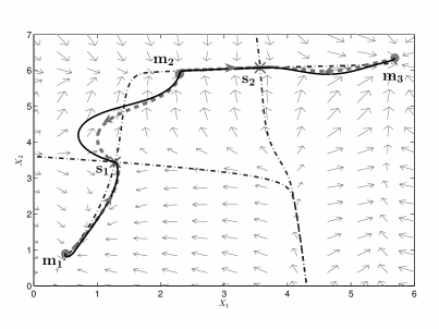
W𝑊W has three local minima m1=(0.4643,0.6985),m2=(2.2038,5.9804)formulae-sequencesubscript𝑚10.46430.6985subscript𝑚22.20385.9804m_{1}=(0.4643,0.6985),m_{2}=(2.2038,5.9804), m3=(5.7109,6.2369)subscript𝑚35.71096.2369m_{3}=(5.7109,6.2369) and two saddle points s1=(1.2841,3.4483),s2=(3.5689,6.0735),formulae-sequencesubscript𝑠11.28413.4483subscript𝑠23.56896.0735s_{1}=(1.2841,3.4483),s_{2}=(3.5689,6.0735),. See Figure 1 below.

In the HMM scheme of the MsGAD, we use the forward Euler solver for the whole system. We take the macro-time step size Δt=0.01Δ𝑡0.01\Delta t=0.01 for both xεsuperscript𝑥𝜀x^{\varepsilon} and vε,wεsuperscript𝑣𝜀superscript𝑤𝜀v^{\varepsilon},w^{\varepsilon} and set τ=1.0𝜏1.0\tau=1.0 and K=1𝐾1K=1 for this example. The micro-time step size is δt=ε×0.01𝛿𝑡𝜀0.01{\delta t}=\varepsilon\times 0.01 and the total sampling time T=10𝑇10T=10 is used to estimate the effective force and the Jacobi matrix. The initial values for x𝑥x are set on three local minima, respectively. The initial values for the directions (v,w)𝑣𝑤(v,w) and the fast processes are arbitrarily chosen. Figure 1 shows the four GAD trajectories of the x𝑥x component (dashed line) starting from three local minima. Depending on the initial values of x𝑥x, these four trajectories converge to the different neighboring saddle points. Two of them which start from m2subscript𝑚2m_{2}, converge to the saddle point s1subscript𝑠1s_{1} and s2subscript𝑠2s_{2} respectively, due to the different initial values for the directions v𝑣v and w𝑤w.

Refer to caption
Figure 1: GAD trajectories from three different local minima (m1,m2subscript𝑚1subscript𝑚2m_{1},m_{2} and m3subscript𝑚3m_{3}) to two different saddle points (s1subscript𝑠1s_{1} and s2subscript𝑠2s_{2}). The flow indicated by the arrows corresponds to the averaged gradient system (4.39). The dash-dotted curves are the stable/unstable manifolds of the two saddle points; they determine the basin boundaries of the three local wells. The thick dashed curves with arrows marked are the trajectories of MsGAD by the HMM. As comparison, the thin solid curves are the trajectories of the GAD directly applied to the closed form (4.39) of the averaged system.

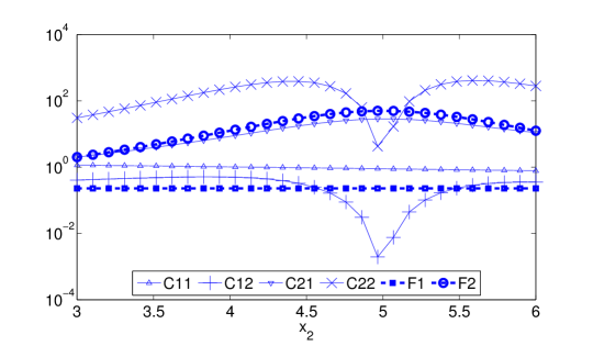
In the end, we conduct a numerical investigation of the variance in estimating the force F=f¯𝐹¯𝑓F=\bar{f} and the Jacobi matrix DF=Dxf¯+C¯𝐷𝐹¯subscript𝐷𝑥𝑓¯𝐶DF=\overline{D_{x}f}+\overline{C}. Specifically, we look at Vary(f(x,y))subscriptVar𝑦𝑓𝑥𝑦\operatorname{Var}_{y}(f(x,y)) and Vary(Dxf(x,y)+C(x,y))subscriptVar𝑦subscript𝐷𝑥𝑓𝑥𝑦𝐶𝑥𝑦\operatorname{Var}_{y}(D_{x}f(x,y)+C(x,y)), where the variance acts component-wisely. The calculation shows that Vary(f(x,y))=Vary(yi2)=12σ4Γi(x)2subscriptVar𝑦𝑓𝑥𝑦subscriptVar𝑦superscriptsubscript𝑦𝑖212superscript𝜎4subscriptΓ𝑖superscript𝑥2\operatorname{Var}_{y}(f(x,y))=\operatorname{Var}_{y}(y_{i}^{2})=\frac{1}{2}\sigma^{4}\Gamma_{i}(x)^{2} and Vary(Dxf(x,y)+C(x,y))=Vary(C(x,y))subscriptVar𝑦subscript𝐷𝑥𝑓𝑥𝑦𝐶𝑥𝑦subscriptVar𝑦𝐶𝑥𝑦\operatorname{Var}_{y}(D_{x}f(x,y)+C(x,y))=\operatorname{Var}_{y}(C(x,y)). For each component, Vary(Cij(x,y))=Vary(fi(x,y)gj(x,y))subscriptVar𝑦subscript𝐶𝑖𝑗𝑥𝑦subscriptVar𝑦subscript𝑓𝑖𝑥𝑦subscript𝑔𝑗𝑥𝑦\operatorname{Var}_{y}(C_{ij}(x,y))=\operatorname{Var}_{y}(f_{i}(x,y)g_{j}(x,y)), one can find that fi(x,y)gj(x,y)=(Di1x1+Di2x2+yi2)(2yj2/σ2+Γj(x))(xj5)subscript𝑓𝑖𝑥𝑦subscript𝑔𝑗𝑥𝑦subscript𝐷𝑖1subscript𝑥1subscript𝐷𝑖2subscript𝑥2superscriptsubscript𝑦𝑖22superscriptsubscript𝑦𝑗2superscript𝜎2subscriptΓ𝑗𝑥subscript𝑥𝑗5f_{i}(x,y)g_{j}(x,y)=-(D_{i1}x_{1}+D_{i2}x_{2}+y_{i}^{2})({2y_{j}^{2}}/{\sigma^{2}}+\Gamma_{j}(x))(x_{j}-5) after plugging in Γi(xi)=2(xi5)Γi2(xi)superscriptsubscriptΓ𝑖subscript𝑥𝑖2subscript𝑥𝑖5subscriptsuperscriptΓ2𝑖subscript𝑥𝑖\Gamma_{i}^{\prime}(x_{i})=-2(x_{i}-5)\Gamma^{2}_{i}(x_{i}). Thus, we have the analytical result that Vary(Cij(x,y))=wij(x)(xj5)2subscriptVar𝑦subscript𝐶𝑖𝑗𝑥𝑦subscript𝑤𝑖𝑗𝑥superscriptsubscript𝑥𝑗52\operatorname{Var}_{y}(C_{ij}(x,y))=w_{ij}(x)(x_{j}-5)^{2}. The expressions of wij(x)subscript𝑤𝑖𝑗𝑥{w_{ij}(x)} are very long and there is no need to write down. The key observation we want to draw attention to is that Vary(Cij(x,y))subscriptVar𝑦subscript𝐶𝑖𝑗𝑥𝑦\operatorname{Var}_{y}(C_{ij}(x,y)) is mainly dominated by the term (xj5)2superscriptsubscript𝑥𝑗52(x_{j}-5)^{2}, while the variance Vary(fi(x,y))subscriptVar𝑦subscript𝑓𝑖𝑥𝑦\operatorname{Var}_{y}(f_{i}(x,y)) is proportional to Γi(xi)=(1+(xi5)2)1subscriptΓ𝑖subscript𝑥𝑖superscript1superscriptsubscript𝑥𝑖521\Gamma_{i}(x_{i})=(1+(x_{i}-5)^{2})^{-1}. In Figure 2, we plot the variance of all components for the force and the covariance matrix and it clearly shows that the variance of Ci2subscript𝐶𝑖2C_{i2} near x25subscript𝑥25x_{2}\approx 5 are distinctively different from that of F𝐹F or the other two components. Therefore, there seems no general conclusion that the variance of the Jacobi matrix would be larger than the force due to the non-trivial dependency of μxsubscript𝜇𝑥\mu_{x} on x𝑥x.

Refer to caption
Figure 2: The variances of the estimator for the effective force F𝐹F and the Jacobi matrix DF𝐷𝐹DF. In our example, the variance of DF𝐷𝐹DF equals the variance of C𝐶C. The plot is the variance for each component along a vertical line segment in 𝒳𝒳\mathcal{X} plane with x2[3,6]subscript𝑥236x_{2}\in[3,6] and x1=1.2841subscript𝑥11.2841x_{1}=1.2841. The saddle point s1subscript𝑠1s_{1} is on this line segment.

4.2 A coupled Allen-Cahn system

Our second example is a system of stochastic partial differential equations of (uε(x,t),ϕε(x,t))superscript𝑢𝜀𝑥𝑡superscriptitalic-ϕ𝜀𝑥𝑡(u^{\varepsilon}(x,t),\phi^{\varepsilon}(x,t)) in the Hilbert space L2([0,1])superscript𝐿201L^{2}([0,1]), satisfying Allen-Cahn-type equations with Neumann boundary condition:

tuεsubscript𝑡superscript𝑢𝜀\displaystyle\partial_{t}u^{\varepsilon} =κ2Δuε+uε(uε)3+μϕε,absentsuperscript𝜅2Δsuperscript𝑢𝜀superscript𝑢𝜀superscriptsuperscript𝑢𝜀3𝜇superscriptitalic-ϕ𝜀\displaystyle=\kappa^{2}\Delta u^{\varepsilon}+u^{\varepsilon}-(u^{\varepsilon})^{3}+\mu\phi^{\varepsilon}, (4.40a)
tϕεsubscript𝑡superscriptitalic-ϕ𝜀\displaystyle\partial_{t}\phi^{\varepsilon} =1ε[Δϕεϕε+μuε]+σεW˙(t),absent1𝜀delimited-[]Δsuperscriptitalic-ϕ𝜀superscriptitalic-ϕ𝜀𝜇superscript𝑢𝜀𝜎𝜀˙𝑊𝑡\displaystyle=\frac{1}{\varepsilon}[\Delta\phi^{\varepsilon}-\phi^{\varepsilon}+\mu u^{\varepsilon}]+\frac{\sigma}{\sqrt{\varepsilon}}\dot{W}(t), (4.40b)

where Δ=x2Δsubscriptsuperscript2𝑥\Delta=\partial^{2}_{x} and W(t)𝑊𝑡W(t) is an L2([0,1])superscript𝐿201L^{2}([0,1])-valued Wiener process with a positive-definite (spatial) covariance operator Q𝑄Q. W˙˙𝑊\dot{W} is white noise in time. κ𝜅\kappa is the diffusion coefficient in slow dynamics and μ𝜇\mu is the coupling constant between the slow and the fast dynamics. σ𝜎\sigma is the noise intensity. For any fixed uε=u,superscript𝑢𝜀𝑢u^{\varepsilon}=u, the equilibrium distribution of the SPDE (4.40b) is the Gaussian measure 𝒩(μ(IΔ)1u,σ2(IΔ)1Q/2)𝒩𝜇superscript𝐼Δ1𝑢superscript𝜎2superscript𝐼Δ1𝑄2\mathcal{N}(\mu(I-\Delta)^{-1}u,{\sigma^{2}(I-\Delta)^{-1}Q}/{2}) on the Cameron–Martin space. We simply choose Q𝑄Q as identity, i.e., formally, W˙˙𝑊\dot{W} is the spatio-temporal white noise. Then, it is easy to see that the averaged equation for the limit solution u¯¯𝑢\bar{u} is

tu¯=κ2Δu¯+u¯u¯3+μ2(IΔ)1u¯,subscript𝑡¯𝑢superscript𝜅2Δ¯𝑢¯𝑢superscript¯𝑢3superscript𝜇2superscript𝐼Δ1¯𝑢\displaystyle\partial_{t}\bar{u}=\kappa^{2}\Delta\bar{u}+\bar{u}-\bar{u}^{3}+\mu^{2}(I-\Delta)^{-1}\bar{u}, (4.41a)
u¯n|x=0=0,u¯n|x=1=0.formulae-sequenceevaluated-at¯𝑢𝑛𝑥00evaluated-at¯𝑢𝑛𝑥10\displaystyle\frac{\partial\bar{u}}{\partial\vec{n}}\Big{|}_{x=0}=0,\quad\frac{\partial\bar{u}}{\partial\vec{n}}\Big{|}_{x=1}=0. (4.41b)

We can find an energy functional U(u,ϕ)𝑈𝑢italic-ϕU(u,\phi) jointly for the pair (u,ϕ)𝑢italic-ϕ(u,\phi):

U(u,ϕ)=Ωκ22ux2+14(u21)2μuϕ+12ϕx2+12ϕ2dx.𝑈𝑢italic-ϕsubscriptΩsuperscript𝜅22superscriptsubscript𝑢𝑥214superscriptsuperscript𝑢212𝜇𝑢italic-ϕ12superscriptsubscriptitalic-ϕ𝑥212superscriptitalic-ϕ2d𝑥U(u,\phi)=\int_{\Omega}\frac{\kappa^{2}}{2}u_{x}^{2}+\frac{1}{4}(u^{2}-1)^{2}-\mu u\phi+\frac{1}{2}\phi_{x}^{2}+\frac{1}{2}\phi^{2}~{}\mathrm{d}x. (4.42)

Since this is a gradient system, the corresponding MsGAD only involves one direction (see Section 3):

tuεsubscript𝑡superscript𝑢𝜀\displaystyle\partial_{t}{u}^{\varepsilon} =δuU(uε,ϕε)+2δuU(uε,ϕε),vεvε,vεvε,absentsubscript𝛿𝑢𝑈superscript𝑢𝜀superscriptitalic-ϕ𝜀2subscript𝛿𝑢𝑈superscript𝑢𝜀superscriptitalic-ϕ𝜀superscript𝑣𝜀superscript𝑣𝜀superscript𝑣𝜀superscript𝑣𝜀\displaystyle=-\delta_{u}U(u^{\varepsilon},\phi^{\varepsilon})+2\frac{\left\langle\delta_{u}U(u^{\varepsilon},\phi^{\varepsilon}),v^{\varepsilon}\right\rangle}{\left\langle v^{\varepsilon},v^{\varepsilon}\right\rangle}v^{\varepsilon}, (4.43a)
tϕεsubscript𝑡superscriptitalic-ϕ𝜀\displaystyle\partial_{t}{\phi}^{\varepsilon} =1εδϕU(uε,ϕε)+σεW˙(t),absent1𝜀subscript𝛿italic-ϕ𝑈superscript𝑢𝜀superscriptitalic-ϕ𝜀𝜎𝜀˙𝑊𝑡\displaystyle=-\frac{1}{\varepsilon}\delta_{\phi}U(u^{\varepsilon},\phi^{\varepsilon})+\frac{\sigma}{\sqrt{\varepsilon}}\dot{W}(t), (4.43b)
tvεsubscript𝑡superscript𝑣𝜀\displaystyle\partial_{t}{v}^{\varepsilon} =δu2U(uε,ϕε)vε+Cvεαεvε,absentsuperscriptsubscript𝛿𝑢2𝑈superscript𝑢𝜀superscriptitalic-ϕ𝜀superscript𝑣𝜀𝐶superscript𝑣𝜀superscript𝛼𝜀superscript𝑣𝜀\displaystyle=-\delta_{u}^{2}U(u^{\varepsilon},\phi^{\varepsilon})v^{\varepsilon}+Cv^{\varepsilon}-\alpha^{\varepsilon}v^{\varepsilon}, (4.43c)

where δuUsubscript𝛿𝑢𝑈\delta_{u}U and δϕUsubscript𝛿italic-ϕ𝑈\delta_{\phi}U are the Fréchet derivative of U(u,ϕ)𝑈𝑢italic-ϕU(u,\phi). δu2Usubscriptsuperscript𝛿2𝑢𝑈\delta^{2}_{u}U is the Hessian. Here C=2σ2δuUδuU+2σ2δuU¯δuU¯.𝐶tensor-product2superscript𝜎2subscript𝛿𝑢𝑈subscript𝛿𝑢𝑈tensor-product2superscript𝜎2¯subscript𝛿𝑢𝑈¯subscript𝛿𝑢𝑈C=-\frac{2}{\sigma^{2}}{\delta_{u}U\otimes\delta_{u}U}+\frac{2}{\sigma^{2}}\overline{\delta_{u}U}\otimes\overline{\delta_{u}U}.

In this example, the parameters are set as κ=0.01𝜅0.01\kappa=0.01, σ=0.3𝜎0.3\sigma=0.3 and μ=1𝜇1\mu=1. The two local minima of the effective dynamics are u±1𝑢plus-or-minus1u\equiv\pm 1 for μ=0𝜇0\mu=0, and u±1.4142𝑢plus-or-minus1.4142u\equiv\pm 1.4142 for μ=1𝜇1\mu=1, respectively. The saddle points are shown in Figure 3.
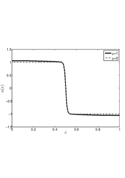
Refer to caption
Refer to caption

(a)                                                     (b)

Figure 3: Two types of index-1 saddle points for μ=0𝜇0\mu=0 (dashed lines) and μ=1𝜇1\mu=1 (solid lines). The saddle point in (a) has a lower energy than the saddle point in (b).

The equation (4.43) are solved by the HMM and the SCM. The time-discrerization scheme for the equation (4.43a) is a convex-splitting scheme for saddle point search ([15]) to allow a stable time step size ΔtΔ𝑡\Delta t. The spatial discretization is the central finite difference method with the uniform mesh grid size Δx=1/200Δ𝑥1200\Delta x=1/200. The term δu2U(u,ϕ)vsuperscriptsubscript𝛿𝑢2𝑈𝑢italic-ϕ𝑣\delta_{u}^{2}U(u,\phi)v in (4.43) is calculated by finite difference approximation

δu2U(u,ϕ)v=1h[δuU(u+hv,ϕ)δuU(u,ϕ)]superscriptsubscript𝛿𝑢2𝑈𝑢italic-ϕ𝑣1delimited-[]subscript𝛿𝑢𝑈𝑢𝑣italic-ϕsubscript𝛿𝑢𝑈𝑢italic-ϕ\delta_{u}^{2}U(u,\phi)v=\frac{1}{h}[\delta_{u}U(u+hv,\phi)-\delta_{u}U(u,\phi)]

with h=0.0010.001h=0.001.

For the seamless coupling method to solve the MsGAD (4.43), according to Section 2.2.2, the boosted system is

tuεsubscript𝑡superscript𝑢𝜀\displaystyle\partial_{t}{u}^{\varepsilon} =δuU(uε,ϕε)+2δuU(uε,ϕε),vεvε,vεvε,absentsubscript𝛿𝑢𝑈superscript𝑢𝜀superscriptitalic-ϕ𝜀2subscript𝛿𝑢𝑈superscript𝑢𝜀superscriptitalic-ϕ𝜀superscript𝑣𝜀superscript𝑣𝜀superscript𝑣𝜀superscript𝑣𝜀\displaystyle=-\delta_{u}U(u^{\varepsilon},\phi^{\varepsilon})+2\frac{\left\langle\delta_{u}U(u^{\varepsilon},\phi^{\varepsilon}),v^{\varepsilon}\right\rangle}{\left\langle v^{\varepsilon},v^{\varepsilon}\right\rangle}v^{\varepsilon}, (4.44a)
tϕεsubscript𝑡superscriptitalic-ϕ𝜀\displaystyle\partial_{t}{\phi}^{\varepsilon} =1ελδϕU(uε,ϕε)+σελW˙1(t),absent1𝜀𝜆subscript𝛿italic-ϕ𝑈superscript𝑢𝜀superscriptitalic-ϕ𝜀𝜎𝜀𝜆subscript˙𝑊1𝑡\displaystyle=-\frac{1}{\varepsilon\lambda}\delta_{\phi}U(u^{\varepsilon},\phi^{\varepsilon})+\frac{\sigma}{\sqrt{\varepsilon\lambda}}\dot{W}_{1}(t), (4.44b)
tψεsubscript𝑡superscript𝜓𝜀\displaystyle\partial_{t}{\psi}^{\varepsilon} =1ελδψU(uε,ψε)+σελW˙2(t),absent1𝜀𝜆subscript𝛿𝜓𝑈superscript𝑢𝜀superscript𝜓𝜀𝜎𝜀𝜆subscript˙𝑊2𝑡\displaystyle=-\frac{1}{\varepsilon\lambda}\delta_{\psi}U(u^{\varepsilon},\psi^{\varepsilon})+\frac{\sigma}{\sqrt{\varepsilon\lambda}}\dot{W}_{2}(t), (4.44c)
tvεsubscript𝑡superscript𝑣𝜀\displaystyle\partial_{t}{v}^{\varepsilon} =δu2U(uε,ϕε)vε+f(uε,ϕε)g(uε,ϕε),vεabsentsuperscriptsubscript𝛿𝑢2𝑈superscript𝑢𝜀superscriptitalic-ϕ𝜀superscript𝑣𝜀𝑓superscript𝑢𝜀superscriptitalic-ϕ𝜀𝑔superscript𝑢𝜀superscriptitalic-ϕ𝜀superscript𝑣𝜀\displaystyle=-\delta_{u}^{2}U(u^{\varepsilon},\phi^{\varepsilon})v^{\varepsilon}+f(u^{\varepsilon},\phi^{\varepsilon})\left\langle g(u^{\varepsilon},\phi^{\varepsilon}),v^{\varepsilon}\right\rangle
f(uε,ψε)g(uε,ϕε),vεαεvε,𝑓superscript𝑢𝜀superscript𝜓𝜀𝑔superscript𝑢𝜀superscriptitalic-ϕ𝜀superscript𝑣𝜀superscript𝛼𝜀superscript𝑣𝜀\displaystyle~{}~{}\quad-f(u^{\varepsilon},\psi^{\varepsilon})\left\langle g(u^{\varepsilon},\phi^{\varepsilon}),v^{\varepsilon}\right\rangle-\alpha^{\varepsilon}v^{\varepsilon}, (4.44d)

where W1subscript𝑊1W_{1} and W2subscript𝑊2W_{2} are two iid copies of W𝑊W. ,\left\langle\cdot,\cdot\right\rangle is the inner product in L2([0,1])superscript𝐿201L^{2}([0,1]).

Define the errors as follows,

errH(t)=uH(x,t)u(x)L2,errS(t)=uS(x,t)u(x)L2,formulae-sequencesubscripterr𝐻𝑡subscriptnormsubscript𝑢𝐻𝑥𝑡superscript𝑢𝑥superscript𝐿2subscripterr𝑆𝑡subscriptnormsubscript𝑢𝑆𝑥𝑡superscript𝑢𝑥superscript𝐿2\mbox{err}_{H}(t)=\|u_{H}(x,t)-u^{*}(x)\|_{L^{2}},~{}~{}~{}\quad\mbox{err}_{S}(t)=\|u_{S}(x,t)-u^{*}(x)\|_{L^{2}},

where uH(x,t)subscript𝑢𝐻𝑥𝑡u_{H}(x,t) represents the result of (4.43) solved by the HMM and uS(x,t)subscript𝑢𝑆𝑥𝑡u_{S}(x,t) is the result of (4.44) solved by the SCM. The true solution u(x)superscript𝑢𝑥u^{*}(x) is obtained from the classic GAD applied to the closed form of the averaged system (4.41) with a very fine time step size and a sufficiency small tolerance.

To test our HMM and SCM, we calculate the saddle point with the lowest energy, i.e., the profile in the left panel of Figure 3. The initial guess is the function cos(πx)𝜋𝑥\cos(\pi x).

Refer to caption
Refer to caption

(a)                                            (b)

Figure 4: (a) shows the evolution of the error with the physical time for the classic GAD applied to (4.41) and for the HMM with various sample sizes M=1000𝑀1000M=1000 and 100001000010000. (b) is the decay of the errors with the number of force calculations.

In the HMM, the macro-time step size for uεsuperscript𝑢𝜀u^{\varepsilon} and vεsuperscript𝑣𝜀v^{\varepsilon} is Δt=0.025Δ𝑡0.025\Delta t=0.025 and the micro-time step size for ϕεsuperscriptitalic-ϕ𝜀\phi^{\varepsilon} is δt=0.01×ε𝛿𝑡0.01𝜀\delta t=0.01\times\varepsilon. To demonstrate the effect of the sample size M𝑀M in the HMM, we use different M𝑀M and run the simulation up to the error 104superscript10410^{-4} and plot in Figure 4 the errors w.r.t. the time as well as w.r.t. the number of force calculations (including the cost in calculating the direction variables). It is observed that a smaller sample size leads to a relatively larger fluctuation and the fluctuation appears earlier in time. The reduced cost from a smaller M𝑀M is quite obvious in the subfigure (b). One can expect a further cost reduction if M𝑀M decreases further; but to attain the error as small as 104superscript10410^{-4}, one should either switch to a larger M𝑀M when approaching the saddle point or average the output in time in order to reduce the variance.

Next, we present the details of the SCM and its adaptive version. In the standard SCM, the constant time step size Δ~t=1.0×10²~Δ𝑡1.0superscript102\widetilde{\Delta}t=1.0\times 10^{-2} is applied for all components and ε=1.0×10⁴,λ=10formulae-sequence𝜀1.0superscript104𝜆10\varepsilon=1.0\times 10^{-4},\lambda=10 (or effectively, ε=ελ=1.0×10³superscript𝜀𝜀𝜆1.0superscript103\varepsilon^{\prime}=\varepsilon\lambda=1.0\times 10^{-3}). In the adaptive SCM, the same values of Δ~t~Δ𝑡\widetilde{\Delta}t and εsuperscript𝜀\varepsilon^{\prime} are used up to the time tasubscript𝑡𝑎t_{a}, where the error errSsubscripterr𝑆\mbox{err}_{S} attains a given threshold 102superscript10210^{-2}. From the time tasubscript𝑡𝑎t_{a}, the adaptive time step size Δ~t~Δ𝑡\widetilde{\Delta}t and the adaptive εsuperscript𝜀\varepsilon^{\prime} are then applied. Specifically, we use Δ~tk=k1/2Δ~t~Δsubscript𝑡𝑘superscript𝑘12~Δ𝑡\widetilde{\Delta}t_{k}=k^{-1/2}\widetilde{\Delta}t and εk=k1/2εsubscriptsuperscript𝜀𝑘superscript𝑘12superscript𝜀\varepsilon^{\prime}_{k}=k^{-1/2}\varepsilon^{\prime} where the subindex k𝑘k counts the number of time steps starting from tasubscript𝑡𝑎t_{a}. As stated in Section 2.3, the final output of the SCM and adaptive SCM are the time-averaged solution u~(x,t)1tt0t0tu(x,s)dsapproaches-limit~𝑢𝑥𝑡1𝑡subscript𝑡0superscriptsubscriptsubscript𝑡0𝑡𝑢𝑥𝑠differential-d𝑠\tilde{u}(x,t)\doteq\frac{1}{t-t_{0}}\int_{t_{0}}^{t}u(x,s)\mathrm{d}s, where t0=10subscript𝑡010t_{0}=10 in this example. This continuous-time integral can be easily implemented on the discrete time points in an iterative way.
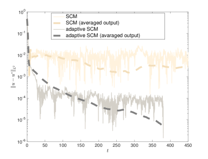
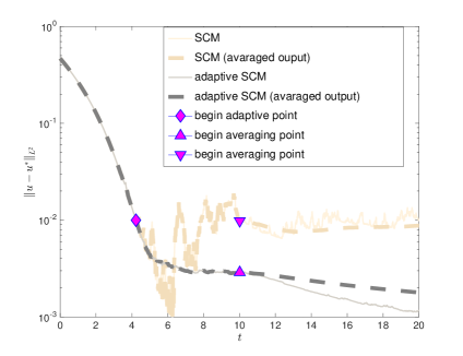
Refer to caption
Refer to caption
Figure 5: The evolution of the error with the time in the seamless coupling method. The right panel is the same plot in the early stage before time t=20𝑡20t=20. The solutions are averaged w.r.t. time after the burn-in time t0=10subscript𝑡010t_{0}=10, which are shown by the two triangular symbols in the plot. The resulted new outputs are shown in dashed thick lines. The value of εsuperscript𝜀\varepsilon^{\prime} and the step size in the adaptive SCM start to decay when the error decreases to 0.010.010.01, which is shown by the diamond symbol in the right plot. The “SCM” means the standard SCM with a fixed εsuperscript𝜀\varepsilon^{\prime} and a constant time step size.

Figure 5 shows the effectiveness of the strategy of decreasing εsuperscript𝜀\varepsilon^{\prime} at time marches. For a fixed ε=103superscript𝜀superscript103\varepsilon^{\prime}=10^{-3}, the error of the SCM can not reach the level of 103superscript10310^{-3}. This discrepancy quickly shrinks when we start to decrease the value of εsuperscript𝜀\varepsilon^{\prime} gradually. The error eventually can decrease to the level 105superscript10510^{-5}. However, this comes with a price: as εsuperscript𝜀\varepsilon^{\prime} shrinks, the problem becomes stiffer and the step size Δ~t~Δ𝑡\widetilde{\Delta}t has to decrease in the same speed. The log-log plot in Figure 6 shows the fast growth of the computational cost when εsuperscript𝜀\varepsilon^{\prime} decreases in the adaptive SCM. Thus, the SCM is not desired for a tiny εsuperscript𝜀\varepsilon^{\prime}, though it can quickly settle down to a region of importance with cheap cost. Figure 6 also illustrates the performance of the HMM and the SCM. Note that since the time step sizes used here in HMM and adaptive SCM are different, this figure is only a qualitative picture. But what we can learn from the above numerical explorations for this example is that the best strategy in practice perhaps is to start with a boosted value εsuperscript𝜀\varepsilon^{\prime} in the adaptive SCM and then switch to the HMM with an adaptive choice of M𝑀M. The optimal choices of the underlying parameters are of both practical importance and theoretic interests and are left for future study.
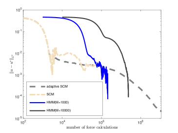
Refer to caption
Figure 6: The illustration of the computational costs for the SCM, the adaptive version of SCM (both with averaged output) and the HMM. The plot is in log-log scale.

5 Conclusion

We have proposed the multiscale method based on the GAD in slow-fast systems. In order to calculate the saddle point of effective dynamics, we derived a new slow-fast system, the MsGAD, whose effective dynamics is consistent with the GAD for the effective dynamics. By applying the multiscale numerical method such as the HMM or the seamless coupling method, we efficiently compute saddle points on averaged dynamics. Some adaptive techniques are presented and illustrated by the numerical experiment.


Appendix: Proof of (2.25).

To show that B𝐵B is the Jacobi matrix DF𝐷𝐹DF, we just need to prove that

(f(x,y)F(x))xlogρ(x,y)ρ(x,y)(dy)=(0yEyf(x,Y~τx)dτ)Dxb(x,y)ρ(x,y)dy.tensor-product𝑓𝑥𝑦𝐹𝑥subscript𝑥𝜌𝑥𝑦𝜌𝑥𝑦d𝑦superscriptsubscript0subscript𝑦superscriptE𝑦𝑓𝑥subscriptsuperscript~𝑌𝑥𝜏differential-d𝜏subscript𝐷𝑥𝑏𝑥𝑦𝜌𝑥𝑦differential-d𝑦\begin{split}\int(f(x,y)-F(x))\otimes\nabla_{x}\log\rho(x,y)\rho(x,y)(\mathrm{d}y)\\ =\int\left(\int_{0}^{\infty}\nabla_{y}\operatorname{E}^{y}f(x,\widetilde{Y}^{x}_{\tau})\mathrm{d}\tau\right)D_{x}b(x,y)\rho(x,y)\mathrm{d}y.\end{split}

To show this matrix equality, we just need to show

(f(x,y)F(x))xρ(x,y),edy=(0yEyf(x,Y~τx)dτ)(Dxb(x,y))eρ(x,y)dy𝑓𝑥𝑦𝐹𝑥subscript𝑥𝜌𝑥𝑦𝑒differential-d𝑦superscriptsubscript0subscript𝑦superscriptE𝑦𝑓𝑥subscriptsuperscript~𝑌𝑥𝜏differential-d𝜏subscript𝐷𝑥𝑏𝑥𝑦𝑒𝜌𝑥𝑦differential-d𝑦\begin{split}&\int(f(x,y)-F(x))\left\langle\nabla_{x}\rho(x,y),e\right\rangle\mathrm{d}y\\ =&\int\left(\int_{0}^{\infty}\nabla_{y}\operatorname{E}^{y}f(x,\widetilde{Y}^{x}_{\tau})\mathrm{d}\tau\right)(D_{x}b(x,y))e\,\rho(x,y)\mathrm{d}y\end{split}

for arbitrary vector e𝑒e. Write the infinitesimal perturbation ρ~:=ρ(x+he,y)ρ(x,y)hxρ(x,y)eassign~𝜌𝜌𝑥𝑒𝑦𝜌𝑥𝑦subscript𝑥𝜌𝑥𝑦𝑒\widetilde{\rho}:=\rho(x+he,y)-\rho(x,y)\approx h\nabla_{x}\rho(x,y)\cdot e and b~(x,y)=b(x+he,y)b(x,y)h(Dxb(x,y))e~𝑏𝑥𝑦𝑏𝑥𝑒𝑦𝑏𝑥𝑦subscript𝐷𝑥𝑏𝑥𝑦𝑒\widetilde{b}(x,y)=b(x+he,y)-b(x,y)\approx h(D_{x}b(x,y))e for h1much-less-than1h\ll 1, and assume e𝑒e is independent of x𝑥x, then the lemma below tells us that

(f(x,y)F(x))xρ(x,y),edy=yu,(Dxb(x,y))eρ(x,y)dy,𝑓𝑥𝑦𝐹𝑥subscript𝑥𝜌𝑥𝑦𝑒differential-d𝑦subscript𝑦𝑢subscript𝐷𝑥𝑏𝑥𝑦𝑒𝜌𝑥𝑦differential-d𝑦\int(f(x,y)-F(x))\left\langle\nabla_{x}\rho(x,y),e\right\rangle\mathrm{d}y=-\int\left\langle\nabla_{y}u,(D_{x}b(x,y))e\right\rangle\rho(x,y)\mathrm{d}y,

where u𝑢u satisfies yu(x,y)=f(x,y)F(x)subscript𝑦𝑢𝑥𝑦𝑓𝑥𝑦𝐹𝑥\mathcal{L}_{y}u(x,y)=f(x,y)-F(x). By the Feymann-Kac formula, we have the representation u(x,y)=0Ey[f(x,Y~tx)+F(x)]dt𝑢𝑥𝑦superscriptsubscript0superscriptE𝑦𝑓𝑥subscriptsuperscript~𝑌𝑥𝑡𝐹𝑥differential-d𝑡u(x,y)=\int_{0}^{\infty}\operatorname{E}^{y}[-f(x,\widetilde{Y}^{x}_{t})+F(x)]\mathrm{d}t, so yu=0yEy[f(x,Y~tx)]dtsubscript𝑦𝑢superscriptsubscript0subscript𝑦superscriptE𝑦𝑓𝑥subscriptsuperscript~𝑌𝑥𝑡differential-d𝑡\nabla_{y}u=-\int_{0}^{\infty}\nabla_{y}\operatorname{E}^{y}[f(x,\widetilde{Y}^{x}_{t})]\mathrm{d}t. This completes our proof.

Lemma 5.1.

If ρ(y)𝜌𝑦\rho(y) is the unique equilibrium probability density function of the SDE

dY=b(Y)dt+σ(Y)dW,d𝑌𝑏𝑌d𝑡𝜎𝑌d𝑊\mathrm{d}Y=b(Y)\mathrm{d}t+\sigma(Y)\mathrm{d}W,

\mathcal{L} is the infinitesimal generator, and the infinitesimal perturbation is applied for the drift term: bb+b~𝑏𝑏~𝑏b\to b+\widetilde{b} and the diffusion term aσσTa+a~approaches-limit𝑎𝜎superscript𝜎T𝑎~𝑎a\doteq\sigma\sigma^{\textsf{T}}\to a+\widetilde{a}, where b~~𝑏\widetilde{b} and a~~𝑎\widetilde{a} are small terms, and let Θθ(y)ρ(y)dyapproaches-limitΘ𝜃𝑦𝜌𝑦differential-d𝑦\Theta\doteq\int\theta(y)\rho(y)\mathrm{d}y, then the perturbation of ΘΘ\Theta is

δΘθ(y)ρ~(y)dy=b~(ρu)(y)dy12a~:ρu(y)dy,:approaches-limit𝛿Θ𝜃𝑦~𝜌𝑦differential-d𝑦~𝑏𝜌𝑢𝑦differential-d𝑦12~𝑎𝜌𝑢𝑦d𝑦\delta\Theta\doteq\int\theta(y)\widetilde{\rho}(y)\mathrm{d}y=-\int\widetilde{b}\cdot(\rho\nabla u)(y)\mathrm{d}y-\frac{1}{2}\int\widetilde{a}:\rho\nabla\nabla u(y)\mathrm{d}y,

where u𝑢u is the solution of the adjoint equation u=θ(y)Θ𝑢𝜃𝑦Θ\mathcal{L}u=\theta(y)-\Theta and decays to 00 at infinity.

Proof: The infinitesimal generator is =b(y)+12a(y)::𝑏𝑦12𝑎𝑦\mathcal{L}=b(y)\cdot\nabla+\frac{1}{2}a(y):\nabla\nabla. The density ρ𝜌\rho satisfies the equation ρ=0superscript𝜌0\mathcal{L}^{*}\rho=0, where superscript\mathcal{L}^{*} is the adjoint of \mathcal{L}. By linearizing the perturbed equation, we have ρ~=(ρb~):(ρa~):superscript~𝜌𝜌~𝑏𝜌~𝑎\mathcal{L}^{*}\widetilde{\rho}=\nabla\cdot(\rho\widetilde{b})-\nabla\nabla:(\rho\widetilde{a}). Multiply this equation by u𝑢u, then from the integration by parts, we have δΘ=ρ~(y)θ(y)dy=ρ~(y)udy=b~(ρu)(y)dy12a~:ρu(y)dy.:𝛿Θ~𝜌𝑦𝜃𝑦differential-d𝑦~𝜌𝑦𝑢differential-d𝑦~𝑏𝜌𝑢𝑦differential-d𝑦12~𝑎𝜌𝑢𝑦d𝑦\delta\Theta=\int\widetilde{\rho}(y)\theta(y)\mathrm{d}y=\int\widetilde{\rho}(y)\mathcal{L}u\mathrm{d}y=-\int\widetilde{b}\cdot(\rho\nabla u)(y)\mathrm{d}y-\frac{1}{2}\int\widetilde{a}:\rho\nabla\nabla u(y)\mathrm{d}y.

References

  • [1] J. M. Bofill and W. Quapp, The variational nature of the gentlest ascent dynamics and the relation of a variational minimum of a curve and the minimum energy path, Theoretical Chemistry Accounts, 135 (2015), pp. 1–14.
  • [2] J. M. Bofill, W. Quapp, and E. Bernuz, Some remarks on the model of the extended gentlest ascent dynamics, Journal of Mathematical Chemistry, 53 (2014), pp. 41–57.
  • [3] F. Bouchet, T. Grafke, T. Tangarife, and E. Vanden-Eijnden, Large deviations in fast–slow systems, Journal of Statistical Physics, 162 (2016), pp. 793–812.
  • [4] G. M. Crippen and H. A. Scheraga, Minimization of polypeptide energy : XI. the method of gentlest ascent, Arch. Biochem. Biophys., 144 (1971), pp. 462–466.
  • [5] W. E, Principle of Multiscale Modeling, Cambridge University Press, 2011.
  • [6] W. E and B. Engquist, The heterogeneous multiscale methods, Commun. Math. Sci., 1 (2003), pp. 87–132.
  • [7] W. E, B. Engquist, X. Li, W. Ren, and E. Vanden-Eijnden, The heterogeneous multiscale method: A review, Commun. Comput. Phys., (2007), p. 2007.
  • [8] W. E, W. Ren, and E. Vanden-Eijnden, A general strategy for designing seamless multiscale methods, Journal of Computational Physics, 228 (2009), pp. 5437 – 5453.
  • [9] W. E and E. Vanden-Eijnden, Metastability, conformation dynamics, and transition pathways in complex systems, in Multiscale Modelling and Simulation, S. Attinger and P. Koumoutsakos, eds., vol. 39 of Lecture Notes in Computational Science and Engineering, Springer Berlin Heidelberg, 2004, pp. 35–68.
  • [10] W. E and X. Zhou, The gentlest ascent dynamics, Nonlinearity, 24 (2011), p. 1831.
  • [11] W. E, X. Zhou, and X. Cheng, Subcritical bifurcation in spatially extended systems, Nonlinearity, 25 (2012), p. 761.
  • [12] M. I. Freidlin and A. D. Wentzell, Random Perturbations of Dynamical Systems, Grundlehren der mathematischen Wissenschaften, Springer-Verlag, New York, 3 ed., 2012.
  • [13] W. Gao, J. Leng, and X. Zhou, An iterative minimization formulation for saddle point search, SIAM J. Numer. Anal., 53 (2015), pp. 1786–1805.
  • [14]  , Iterative minimization algorithm for efficient calculations of transition states, Journal of Computational Physics, 309 (2016), pp. 69 – 87.
  • [15] S. Gu and X. Zhou, Convex splitting method for the calculation of transition states of energy functional., arXiv:1610.07153, (2016).
  • [16] G. Henkelman and H. Jónsson, A dimer method for finding saddle points on high dimensional potential surfaces using only first derivatives, J. Chem. Phys., 111 (1999), pp. 7010–7022.
  • [17] M. Iannuzzi, A. Laio, and M. Parrinello, Efficient exploration of reactive potential energy surfaces using Car-Parrinello molecular dynamics, Phys. Rev. Lett., 90 (2003), p. 238302.
  • [18] D. Kelly and E. Vanden-Eijnden, Fluctuations in the heterogeneous multiscale methods for fast-slow systems, arXiv:1601.02147, (2016).
  • [19] R. Z. Khasaminskii, A limit theorem for the solutions of differential equations with random right-hand sides, Theory of Probability & Its Applications, 11 (1966), pp. 390–406.
  • [20] R. Z. Khasminskii and G. Yin, On averaging principles: An asymptotic expansion approach, SIAM Journal on Mathematical Analysis, 35 (2004), pp. 1534–1560.
  • [21] P. Kloeden and E. Platen, Numerical Solution of Stochastic Differential Equations, Stochastic Modelling and Applied Probability, Springer Berlin Heidelberg, 2013.
  • [22] A. Laio and M. Parrinello, Escaping free-energy minima, Proceedings of the National Academy of Sciences, 99 (2002), pp. 12562–12566.
  • [23] B. Leimkuhler, C. Matthews, and G. Stoltz, The computation of averages from equilibrium and nonequilibrium langevin molecular dynamics, IMA Journal of Numerical Analysis, 36 (2016), pp. 13–79.
  • [24] C. Li, J. Lu, and W. Yang, Gentlest ascent dynamics for calculating first excited state and exploring energy landscape of Kohn-Sham density functionals, The Journal of Chemical Physics, 143 (2015), p. 224110.
  • [25] L. Maragliano, A. Fischer, E. Vanden-Eijnden, and G. Ciccotti, String method in collective variables: Minimum free energy paths and isocommittor surfaces, J. Chem. Phys., 125 (2006), p. 024106.
  • [26] N. Mousseau and G. Barkema, Traveling through potential energy surfaces of disordered materials: the activation-relaxation technique, Phys. Rev. E, 57 (1998), p. 2419.
  • [27] G. Papanicolaou, Introduction to the asymptotic analysis of stochastic equations, in Lectures in Appl. Math., vol. 16, Amer. Math. Soc., Providence, R.I., 1977, pp. 109–147.
  • [28] P. Rein ten Wolde, M. J. Ruiz-Montero, and D. Frenkel, Numerical calculation of the rate of crystal nucleation in a Lennard-Jones system at moderate undercooling, J. Chem. Phys., 104 (1996), pp. 9932–9947.
  • [29] A. Samanta, M. Chen, T.-Q. Yu, M. Tuckerman, and W. E, Sampling saddle points on a free energy surface, J. Chem. Phys., 140 (2014), p. 164109.
  • [30] A. Samanta and W. E, Atomistic simulations of rare events using gentlest ascent dynamics, J. Chem. Phys., 136 (2012), p. 124104.
  • [31] A. Veretennikov, On large deviations for SDEs with small diffusion and averaging, Stoch. Proc. Appl., 89 (2000), pp. 69–79.
  • [32] D. J. Wales, Energy Landscapes with Application to Clusters, Biomolecules and Glasses, Cambridge University Press, 2003.
  • [33] J. Zhang and Q. Du, Shrinking dimer dynamics and its applications to saddle point search, SIAM J. Numer. Anal., 50 (2012), pp. 1899–1921.
  • [34] L. Zhang, Q. Du, and Z. Zheng, Optimization-based shrinking dimer method for finding transition states, SIAM Journal on Scientific Computing, 38 (2016), pp. A528–A544.
  • [35] L. Zhang, W. Ren, A. Samanta, and Q. Du, Recent developments in computational modeling of nucleation in phase transformations, npj Computational Materials, 2 (2016), p. 16003.
  • [36] L. Zhang, J. Zhang, and Q. Du, Finding critical nuclei in phase transformations by shrinking dimer dynamics and its variants, Communications in Computational Physics, 16 (2014), pp. 781–798.