Small-sample testing inference in symmetric and log-symmetric linear regression models

Abstract

This paper deals with the issue of testing hypothesis in symmetric and log-symmetric linear regression models in small and moderate-sized samples. We focus on four tests, namely the Wald, likelihood ratio, score, and gradient tests. These tests rely on asymptotic results and are unreliable when the sample size is not large enough to guarantee a good agreement between the exact distribution of the test statistic and the corresponding chi-squared asymptotic distribution. Bartlett and Bartlett-type corrections typically attenuate the size distortion of the tests. These corrections are available in the literature for the likelihood ratio and score tests in symmetric linear regression models. Here, we derive a Bartlett-type correction for the gradient test. We show that the corrections are also valid for the log-symmetric linear regression models. We numerically compare the various tests, and bootstrapped tests, through simulations. Our results suggest that the corrected and bootstrapped tests exhibit type I probability error closer to the chosen nominal level with virtually no power loss. The analytically corrected tests, including the Bartlett-corrected gradient test derived in this paper, perform as well as the bootstrapped tests with the advantage of not requiring computationally-intensive calculations. We present two real data applications to illustrate the usefulness of the modified tests.

Keywords: Symmetric regression models; Bartlett correction; Bartlett-type correction; Bootstrap; Log-symmetric regression models; gradient statistic; score statistic; likelihood ratio statistic; Wald statistic.

1 Introduction

Normal linear regression models are widely employed in empirical research. There is a vast literature on extensions of these models to deal with non-normal errors. In particular, much attention has been paid to symmetric linear and non-linear regression models; see Villegas et al. (2013), Lemonte (2012), Paula and Cysneiros (2009), Cysneiros et al. (2007), and Galea et al. (2005). The idea is to replace the assumed normal distribution for the error by a wide class of symmetric distributions that encompasses distributions with heavier and lighter tails than the normal distribution. Some examples are the Student-t, type I logistic, type II logistic, contaminated normal, power exponential and slash distributions.

When dealing with positive, possibly skewed, data it is common practice to log-transform the observations and model the transformed data using a normal linear regression model. The corresponding model for the original data involves a multiplicative error term with a log-normal distribution. This limitation is relaxed in the class of the log-symmetric linear regression models (Vanegas and Paula, 2015a, b). It replaces the log-normal distribution by the class of log-symmetric distributions, which includes, for instance, the log-Student-t, type I log-logistic, type II log-logistic, log-contaminated-normal, log-power-exponential, and log-slash distributions.

Hypothesis testing in parametric models usually employ one of the three classic statistics, referred to as the “Holy Trinity” in the statistical literature, namely the Wald, likelihood ratio and Rao score statistics. Recently, the gradient statistic (Terrell, 2002) has received attention. It is attractive because it is very simple to compute (Rao, 2005, Section 1.8). It only involves the score vector and the maximum likelihood estimates (unrestricted and restricted to the null hypothesis) of the parameter vector. Unlike the Wald and score statistics, the gradient statistic does not require the information matrix, it does not involve matrix inversion, and it shares the same first order asymptotic properties with the other three statistics (Lemonte and Ferrari, 2012). The four statistics differ in the second-order properties and may have considerably different behavior in finite samples.

Let ${\cal H}_{0}$ be the null hypothesis to be tested against the alternative hypothesis ${\cal H}_{1}$. Under usual regularity conditions for likelihood inference, the Wald, likelihood ratio, score and gradient statistics have an asymptotic $\chi^{2}_{q}$ distribution, where $q$ is the number of parameters fixed at ${\cal H}_{0}$. When the sample size is small or moderate, the $\chi^{2}_{q}$ approximation may be poor, and the true, unknown, type I probability error may be much larger than the nominal level of the test. Corrections to the test statistics have been proposed to attenuate this distortion. A Bartlett correction to the likelihood ratio statistic was first proposed by Bartlett (1937) and later studied in full generality by Lawley (1956). Cordeiro and Ferrari (1991) derived a Bartlett-type correction to the score statistic. Recently, Vargas et al. (2013) obtained a Bartlett-type correction to the gradient statistic. Typically, the order of approximation error of the null distributions of the statistics by the $\chi^{2}_{q}$ distribution is reduced from $O(n^{-1})$ to $O(n^{-2})$ when the corrections are applied. These corrections have been frequently employed in many parametric models; see, for instance, Chan et al. (2014), da Silva-Júnior et al. (2014), Vargas et al. (2014), Bayer and Cribari-Neto (2013), Lemonte and Ferrari (2011), Lemonte et al. (2010), Lagos et al. (2010), da Silva and Cordeiro (2009), Melo et al. (2009), and Barroso and Cordeiro (2005). Simulation experiments reported in these papers suggest that the size distortions of the tests may be substantially reduced in small and moderate-sized samples when the corrections are applied.

Some works have focused on Bartlett and Bartlett-type corrections in symmetric regression models. Ferrari and Uribe-Opazo (2001) and Cordeiro (2004) obtained a Bartlett correction to the likelihood ratio statistic for linear and nonlinear symmetric regression models, respectively. Uribe-Opazo et al. (2008) and Cysneiros et al. (2010) obtained a Bartlett-type correction to the score statistic in linear and nonlinear symmetric regression models, respectively. In this paper, we derive a Bartlett-type correction to the gradient statistic in symmetric linear regression models. We show that the corrections derived for the symmetric linear regression models are also applicable to the log-symmetric linear regression models. Additionally, we present Monte Carlo experiments to study and compare the finite sample properties of the corrected and uncorrected tests and bootstrapped tests.

This paper is organized as follows. In Section 2 we define the symmetric linear regression models and discuss estimation and hypothesis testing issues. In Section 3 we present a Bartlett correction to the likelihood ratio statistic and a Bartlett-type correction to the score statistic, and derive a Bartlett-type correction to the gradient statistic in the symmetric linear regression models. In Section 4 we present the log-symmetric regression models and show that the results presented in the previous sections are valid in this class of models. In Section 5 we present Monte Carlo simulation results. In Section 6 we present two application in real data sets. Section 7 closes the paper with final remarks.

2 Symmetric linear regression models, estimation and testing

Let $y$ be a continuous random variable having a symmetric distribution with location parameter $\mu\in\mathbb{R}$ and scale parameter $\phi>0$ and probability density function

$$\pi\left(y;\mu,\phi\right)=\dfrac{1}{\phi}h\left(\left(\dfrac{y-\mu}{\phi}\right)^{2}\right),\hskip 28.45274pty\in\mathbb{R},$$ (1)

for some function $h:\mathbb{R}\rightarrow[0,\infty)$, such that $\int_{0}^{\infty}u^{-1/2}h(u)du=1$, called the density generating function. We write $y\sim S(\mu,\phi^{2})$. Different choices for the function $h$ lead to different symmetric distributions; see Table 1 for some examples. Two remarkable examples are the normal and the Student-t distributions. Note that $h$ may depend on extra parameters, for instance, the degrees of freedom parameter of the Student-t distribution. Whenever this is the case, such parameters are assumed to be fixed.

Some well-known properties of the normal distribution are valid for the symmetric distributions. For instance, if $y\sim S(\mu,\phi^{2})$, then $a+by\sim S(a+b\mu,b^{2}\phi^{2})$, with $a$, $b\in\mathbb{R}$, and $b\neq 0$. In particular, $z=(y-\mu)/\phi\sim S(0,1)$ and has probability density function $\pi(z;0,1)=h(z^{2})$, $z\in\mathbb{R}$. Whenever they exist, $E(y)=\mu$ and $\mathrm{Var}(y)=\phi\xi$, where $\xi>0$ is a constant not depending on the parameters. The quantity $\xi$ for some distributions is presented in Table 1. Other results and properties of the symmetric distributions are given in Berkane and Bentler (1986), Rao (1990) and Fang et al. (1990).

Let $y_{1},\ldots,y_{n}$ be independent random variables with $y_{l}\sim S(\mu_{l},\phi^{2})$, for $l=1,\dots n$. The symmetric linear regression models are defined as

$$y_{l}=\bm{x}_{l}^{\top}\bm{\beta}+\phi\,\epsilon_{l},\qquad l=1,\ldots,n,$$ (2)

where $\bm{x}_{l}=(x_{l1},\ldots,x_{lp})^{\top}$ is the vector of covariates associated to the $l$-th observation, $\bm{\beta}=(\beta_{1},\ldots,\beta_{p})^{\top}$ is a vector of unknown parameters and $\epsilon_{1},\ldots,\epsilon_{n}$, are independent random errors with $\epsilon_{l}\sim S(0,1)$. We assume that $\bm{X}=(\bm{x}_{1},\cdots,\bm{x}_{n})$ is a full-rank $n\times p$ matrix, i.e. $\mathrm{rank}(\bm{X})=p$. Additionally, we assume that usual regularity conditions for likelihood inference are valid (Cox and Hinkley, 1974, Chap.9). The assumption that $\epsilon_{l}\sim S(0,1)$ relaxes the normality assumption for the errors allowing distributions with heavier tails (e.g. Student-t, type II logistic, power exponential with $0<k<1$) or lighter tails (e.g. type I logistic, power exponential with $-1<k<0$). The widely employed normal linear regression model is a special case of (2).

The log-likelihood function for $\bm{\theta}=(\bm{\beta}^{\top},\phi)^{\top}$ is

$$l(\bm{\theta})=-n\log(\phi)+\displaystyle{\sum_{l=1}^{n}}g(z_{l}),$$ (3)

with $g(z_{l})=\log h(z_{l}^{2})$ and $z_{l}=(y_{l}-\bm{x}_{l}^{\top}\bm{\beta})/\phi$ being the standardized error associated to the $l$-th observation. The score vector for $\bm{\beta}$ and $\phi$ is given by $\bm{U}(\bm{\theta})=(\bm{U}_{\bm{\beta}}(\bm{\theta})^{\top},U_{\phi}(\bm{\theta}))^{\top}$ with

$$\bm{U}_{\bm{\beta}}(\bm{\theta})=\phi^{-2}\bm{X}^{\top}\bm{W}(\bm{y}-\bm{X}\bm{\beta}),\ \ \ U_{\phi}(\bm{\theta})=\phi^{-1}\left(\phi^{-2}(\bm{y}-\bm{X}\bm{\beta})^{\top}\bm{W}(\bm{y}-\bm{X}\bm{\beta})-n\right),$$

where $\bm{y}=(y_{1},\ldots,y_{n})^{\top}$ and $\bm{W}={\rm diag}\{w_{1},\ldots,w_{n}\}$ with $w_{l}=-2\mathrm{d}\log h(u)/\mathrm{d}u|_{u=z_{l}^{2}}$.

The maximum likelihood estimates of $\bm{\beta}$ and $\phi$, obtained by simultaneously solving the equations $\bm{U}_{\bm{\beta}}(\bm{\theta})=\bm{0}$ and $U_{\phi}(\bm{\theta})=0$, are solutions of $\widehat{\bm{\beta}}=(\bm{X}^{\top}\widehat{\bm{W}}\bm{X})^{-1}\bm{X}^{\top}\widehat{\bm{W}}\bm{y}$ and $\widehat{\phi}^{2}=n^{-1}\widehat{\bm{e}}^{\top}\widehat{\bm{W}}\widehat{\bm{e}}$ with $\widehat{\bm{e}}=\bm{y}-\bm{X}\widehat{\bm{\beta}}$ being the vector of the residuals. For each $l$, $w_{l}$ may be interpreted as the weight of the $l$-th observation in the estimation of the parameters. Table 1 presents $w_{l}$ for some symmetric distributions. Note that the weights of all the observations are the same under the normality assumption for the errors. For the Cauchy, Student-t, type II logistic and power exponential (with $0<k<1$) distributions the weights $w_{l}$ are decreasing functions of $\left|z_{l}\right|$. Hence, the maximum likelihood estimators of $\bm{\beta}$ and $\phi$ are robust to the presence of outliers. For the type-I logistic and power exponential (with $-1<k<0$) distributions, the weights $w_{l}$ are increasing functions of $\left|z_{l}\right|$ because these distributions have lighter tails than the normal distribution.

Table 1: Density generating function, $w$ and $\xi$ for some symmetric distributions.^a

Distribution	$h(u),\ u>0$	$w$	$\xi$	$\delta_{20000}$	$\delta_{20002}$
normal	$\frac{1}{\sqrt{2\pi}}e^{-u/2}$	$1$	$1$	$1$	$3$
Cauchy	$\frac{1}{\pi}(1+u)^{-1}$	$\frac{2}{1+z^{2}}$	does not exist	$\frac{1}{2}$	$\frac{3}{2}$
Student-t	$\frac{\nu^{\nu/2}}{B(1/2,\nu/2)}(\nu+u)^{-\frac{\nu+1}{2}},$	$\frac{\nu+1}{\nu+z^{2}}$	$\frac{\nu}{1+\nu}$, $\nu>2$	$\frac{\nu+1}{\nu+3}$	$\frac{3(\nu+1)}{\nu+3}$
	$\nu>0$
type I logistic	$c\frac{e^{-u}}{(1+e^{-u})^{2}},c\cong 1.4843$	$2\tanh(z^{2}/2)$	$\cong 0.79569$	$\cong 1.47724$	$\cong 4.01378$
type II logistic	$\frac{e^{-\sqrt{u}}}{(1+e^{-\sqrt{u}})^{2}}$	$\frac{e^{-|z|}-1}{|z|(1+e^{-|z|})}$	$\frac{\pi^{2}}{3}$	$\frac{1}{3}$	$\cong 2.42996$
power exponential	$\frac{1}{C(k)}\exp\{-\frac{1}{2}u^{1/(1+k)}\},$	$\frac{1}{(1+k)z^{2k/(1+k)}}$	$2^{1+k}\frac{\Gamma(\frac{3}{2}(1+k))}{\Gamma(\frac{1+k}{2})}$	$2^{1-k}\frac{\Gamma(\frac{3-k}{2})}{(1+k)^{2}\Gamma(\frac{1+k}{2})}$	$\frac{3+k}{1+k}$
	$-1<k\leq 1$
a$B(\cdot,\cdot)$ and $\Gamma(\cdot)$ are the beta and gamma functions, respectively, and $C(k)=\Gamma(1+\frac{1+k}{2})2^{1+(1+k)/2}$.

Let $\delta_{abcde}=E(g^{(1)^{a}}g^{(2)^{b}}g^{(3)^{c}}g^{(4)^{d}}z^{e})$, for $a,b,c,d,e\in\{0,1,2,3,4\}$, $g^{(r)}=\mathrm{d}^{r}g(z)/\mathrm{d}z^{r}$ and $z\sim S(0,1)$. Uribe-Opazo et al. (2008) give the $\delta$’s for some symmetric distributions. The $\delta$’s satisfy regularity relations such as $\delta_{01001}=\delta_{10000}=0$, $\delta_{20000}=-\delta_{01000}$, $\delta_{00010}=-\delta_{10100}$, $\delta_{40000}=-3\delta_{21000}$, $\delta_{01002}=2-\delta_{20002}$, $\delta_{11001}+\delta_{00101}+\delta_{01000}=0$, $2\delta_{00101}+\delta_{00012}+\delta_{10102}=0$, and $3\delta_{01002}+\delta_{11003}+\delta_{00103}=0$. The Fisher information matrix for $\bm{\theta}=(\bm{\beta}^{\top},\phi)^{\top}$ is block diagonal and is given by $\bm{K}={\rm diag}\{\bm{K_{\beta}},{K}_{\phi}\}$, with $\bm{K_{\beta}}=\phi^{-2}\delta_{20000}\bm{X}^{\top}\bm{X}$ and ${K}_{\phi}=n\phi^{-2}(\delta_{20002}-1)$. The quantities $\delta_{20000}$ and $\delta_{20002}$ are given in Table 1 for some distributions. Hence, $\bm{\beta}$ and $\phi$ are globally orthogonal and their maximum likelihood estimators are asymptotically uncorrelated.

The equations $\bm{U}_{\bm{\beta}}(\bm{\theta})=\bm{0}$ and $U{\phi}(\bm{\theta})=0$ cannot be analytically solved, except for the normal model. The Fisher scoring iterative method for estimating $\bm{\beta}$ and $\phi$ may be implemented by iteratively solving

$$\bm{\beta}^{(m+1)} =\bm{\beta}^{(m)}+\frac{1}{\delta_{20000}}(\bm{X}^{\top}\bm{X})^{-1}\bm{X}^{\top}\bm{W}^{(m)}(\bm{y}-\bm{X}\bm{\beta}^{(m)}),$$

$$\phi^{(m+1)} =\phi^{(m)}+\frac{1}{\phi^{(m)}(\delta_{20002}-1)}\left(\frac{1}{n}(\bm{y}-\bm{X}\bm{\beta}^{(m)})\bm{W}^{(m)}(\bm{y}-\bm{X}\bm{\beta}^{(m)})-{\phi^{(m)}}^{2}\right),$$

for $m=0,1,\ldots$. The process may be initialized with $\bm{\beta}^{(0)}=(\bm{X}^{\top}\bm{X})^{-1}\bm{X}^{\top}\bm{y}$, the ordinary least squares estimate of $\bm{\beta}$, and $\phi^{(0)}=((\bm{y}-\bm{X}\bm{\beta}^{(0)})^{\top}(\bm{y}-\bm{X}\bm{\beta}^{(0)})/n)^{1/2}$. Some symmetric distributions can be obtained as a scale mixture of normal distributions, for example, the Student-t and power exponential ($0<k<1$) distributions (Andrews and Mallows, 1974; West, 1987). Hence, the EM algorithm (Dempster et al., 1977) may be used to find the maximum likelihood estimates of the parameters. Estimation in symmetric and log-symmetric models is implemented in the package ssym (Vanegas and Paula, 2015c, d) in R (R Core Team, 2015).

Let $\mathcal{H}_{0}:\bm{\beta}_{1}=\bm{\beta}_{10}$ be the null hypothesis to be tested against $\mathcal{H}_{1}:\bm{\beta}_{1}\neq\bm{\beta}_{10}$, where the vector of unknown parameters $\bm{\beta}$ is partitioned as $\bm{\beta}=(\bm{\beta}_{1}^{\top},\bm{\beta}_{2}^{\top})^{\top}$ with $\bm{\beta}_{1}=(\beta_{1},\dots,\beta_{q})^{\top}$, $\bm{\beta}_{2}=(\beta_{q+1},\dots,\beta_{p})^{\top}$, and $\bm{\beta}_{10}$ is a $q$-vector of fixed constants.The partition of $\bm{\beta}$ induces the following partitions: $\bm{U}_{\bm{\beta}}=(\bm{U}_{\bm{\beta}_{1}}^{\top},\bm{U}_{\bm{\beta}_{2}}^{\top})^{\top}$, with $\bm{U}_{\bm{\beta}_{1}}=\phi^{-2}\bm{X}_{1}^{\top}\bm{W}(\bm{y}-\bm{X}\bm{\beta})$ and $\bm{U}_{\bm{\beta}_{2}}=\phi^{-2}\bm{X}_{2}^{\top}\bm{W}(\bm{y}-\bm{X}\bm{\beta})$, and

$$\bm{K}_{\bm{\beta}}=\begin{bmatrix}\bm{K}_{\bm{\beta}11}&\bm{K}_{\bm{\beta}12}\\ \bm{K}_{\bm{\beta}21}&\bm{K}_{\bm{\beta}22}\end{bmatrix}=\frac{\delta_{20000}}{\phi^{2}}\begin{bmatrix}\bm{X}_{1}^{\top}\bm{X}_{1}&\bm{X}_{1}^{\top}\bm{X}_{2}\\ \bm{X}_{2}^{\top}\bm{X}_{1}&\bm{X}_{2}^{\top}\bm{X}_{2}\end{bmatrix},$$

with the matrix $\bm{X}$ partitioned as $\bm{X}=\bigl{[}\bm{X}_{1}\ \ \bm{X}_{2}\bigr{]}$, where $\bm{X}_{1}$ is an $n\times q$ matrix and $\bm{X}_{2}$ is an $n\times(p-q)$ matrix. To test $\mathcal{H}_{0}:\bm{\beta}_{1}=\bm{\beta}_{10}$ against $\mathcal{H}_{1}:\bm{\beta}_{1}\neq\bm{\beta}_{10}$ the Wald, likelihood ratio, score and gradient statistics may be employed. They are respectively given by

$$S_{\textrm{W}}=\delta_{20000}\widehat{\phi}^{-2}(\widehat{\bm{\beta}}_{1}-\bm{\beta}_{10})^{\top}(\bm{R}^{\top}\bm{R})(\widehat{\bm{\beta}}_{1}-\bm{\beta}_{10}),$$

$$S_{\textrm{LR}}=2\bigl{\{}\ell(\widehat{\bm{\beta}}_{1},\widehat{\bm{\beta}}_{2},\widehat{\phi})-\ell(\bm{\beta}_{10},\widetilde{\bm{\beta}}_{2},\widetilde{\phi})\bigr{\}},$$

$$S_{\textrm{R}}=\frac{1}{\widetilde{\phi}^{2}\delta_{20000}}(\bm{y}-\bm{X}\widetilde{\bm{\beta}})^{\top}\widetilde{\bm{W}}\bm{X}_{1}(\bm{R}^{\top}\bm{R})^{-1}\bm{X}_{1}^{\top}\widetilde{\bm{W}}(\bm{y}-\bm{X}\widetilde{\bm{\beta}}),$$

$$S_{\textrm{T}}=\widetilde{\phi}^{-2}(\bm{y}-\bm{X}\widetilde{\bm{\beta}})^{\top}\widetilde{\bm{W}}{\bm{X}}_{1}(\widehat{\bm{\beta}}_{1}-\bm{\beta}_{10}),$$

where $(\widehat{\bm{\beta}}_{1},\widehat{\bm{\beta}}_{2},\widehat{\phi})$ and $(\bm{\beta}_{10},\widetilde{\bm{\beta}}_{2},\widetilde{\phi})$ are the unrestricted and restricted (to the null hypothesis) maximum likelihood estimator of $(\bm{\beta}_{1},\bm{\beta}_{2},\phi)$, respectively, and $\bm{R}=\bm{X}_{1}-\bm{X}_{2}(\bm{X}_{2}^{\top}\bm{X}_{2})^{-1}\bm{X}_{2}^{\top}\bm{X}_{1}$. Tilde and hat are used to indicate evaluation at $(\widehat{\bm{\beta}}_{1},\widehat{\bm{\beta}}_{2},\widehat{\phi})$ and $(\bm{\beta}_{10},\widetilde{\bm{\beta}}_{2},\widetilde{\phi})$, respectively. Under the null hypothesis, the limiting distribution of the four statistics is $\chi_{q}^{2}$. Note that, unlike the Wald and score statistics, the gradient and likelihood ratio statistics do not involve matrix inversion.

3 Improved tests in symmetric linear regression models

Under usual regularity conditions, the statistics $S_{\textrm{W}}$, $S_{\textrm{LR}}$, $S_{\textrm{R}}$, and $S_{\textrm{T}}$ are asymptotically equivalent. In particular, they all have the same limiting $\chi^{2}_{q}$ distribution with approximation error of order $O(n^{-1})$ under $\mathcal{H}_{0}$. In small and moderate-sized samples, the use of the $\chi^{2}$ approximation may cause considerable type I error probability distortion. Second-order asymptotic theory allows us to derive corrections to the test statistics that attenuate this problem. A Bartlett correction to the likelihood ratio statistic in symmetric linear regression models was obtained by Ferrari and Uribe-Opazo (2001), and a Bartlett-type correction to the score statistic was derived by Uribe-Opazo et al. (2008). In this section, we derive a Bartlett-type correction to the gradient statistic. For this purpose, we make use of the general results in Vargas et al. (2013). Our results are new and represent a significant contribution to improvement of hypothesis testing in symmetric linear regression models.

Define the following matrices: $\bm{Z}=\bm{X}(\bm{X}^{\top}\bm{X})^{-1}\bm{X}^{\top}$, $\bm{Z}_{2}=\bm{X}_{2}(\bm{X}_{2}^{\top}\bm{X}_{2})^{-1}\bm{X}_{2}^{\top}$ (if $q<p$; $\bm{Z}_{2}=\bm{0}_{n\times n}$, if $q=p$), $\bm{Z}_{d}={\rm diag}\{z_{11},\ldots,z_{nn}\}$, $\bm{Z}_{2d}={\rm diag}\{z_{211},\ldots,z_{2nn}\}$. The matrices $\phi^{2}\delta_{20000}^{-1}\bm{Z}$ and $\phi^{2}\delta_{20000}^{-1}\bm{Z}_{2}$ are the asymptotic covariance matrices of $\bm{X}\widehat{\bm{\beta}}$ and $\bm{X}_{2}\widetilde{\bm{\beta}}_{2}$, respectively. Let $\rho_{ZZ}=n\mathrm{tr}(\bm{Z}_{d}\bm{Z}_{d})$, $\rho_{Z_{2}Z_{2}}=n\mathrm{tr}(\bm{Z}_{2d}\bm{Z}_{2d})$, and $\rho_{ZZ_{2}}=n\mathrm{tr}(\bm{Z}_{d}\bm{Z}_{2d})$, where $\mathrm{tr}$ is the trace operator. From the general formulas in Lawley (1956), Ferrari and Uribe-Opazo (2001) obtained a Bartlett correction to the likelihood ratio statistic of $\mathcal{H}_{0}:\bm{\beta}_{1}=\bm{\beta}_{10}$ in symmetric linear regression models as

$$S_{\textrm{LR}}^{*}=S_{\textrm{LR}}(1-a_{{\textrm{LR}}}),$$ (4)

where $a_{{\textrm{LR}}}$ is of order $O(n^{-1})$ and is given by $a_{{\textrm{LR}}}=A_{\textrm{LR}}+A_{{\textrm{LR}},\beta\phi}$, with

$$A_{{\textrm{LR}}} =\frac{d_{0}}{nq}(\rho_{ZZ}-\rho_{Z_{2}Z_{2}}),\hskip 56.9055ptA_{{\textrm{LR}},\beta\phi}=\frac{d_{1}}{n}+\frac{d_{2}}{n}\frac{2p-q}{2},$$

and

$$d_{0}=\frac{\delta_{00010}}{4\delta^{2}_{20000}},\qquad d_{1}=-\frac{m_{2}m_{3}}{2m^{2}_{1}}-\frac{2m_{3}+m^{2}_{3}+m_{4}}{2m_{1}},\qquad d_{2}=-\frac{m^{2}_{3}}{2m_{1}},$$

where

$$m_{1}=\delta_{01002}-1,\hskip 14.22636ptm_{2}=4-\delta_{00103}-6\delta_{01002},\hskip 14.22636ptm_{3}=\frac{\delta_{00101}+2\delta_{01000}}{\delta_{20000}},\hskip 14.22636ptm_{4}=\frac{\delta_{00012}-6\delta_{11001}}{\delta_{20000}}.$$

When $\phi$ is known, $A_{{\textrm{LR}},\beta\phi}=0$. Under the null hypothesis the corrected statistic $S_{\textrm{LR}}^{*}$ has an asymptotic $\chi_{q}^{2}$ distribution with approximation error of order $O(n^{-2})$. Hence, the correction factor reduces the approximation error from $O(n^{-1})$ to $O(n^{-2})$.

A Bartlett-type correction to the score test of $\mathcal{H}_{0}:\bm{\beta}_{1}=\bm{\beta}_{10}$ in symmetric linear regression models has been derived by Uribe-Opazo et al. (2008) from the general results of Cordeiro and Ferrari (1991). The Bartlett-type corrected score statistic is given by

$${S}_{{\textrm{R}}}^{*}={S}_{{\textrm{R}}}\bigl{[}1-\bigl{(}{c}_{{\textrm{R}}}+{b}_{{\textrm{R}}}{S}_{\textrm{R}}+{a}_{{\textrm{R}}}{S}_{{\textrm{R}}}^{2}\bigr{)}\bigr{]},$$ (5)

where ${a_{\textrm{R}}}$, ${b_{\textrm{R}}}$, and ${c_{\textrm{R}}}$ are of order $O(n^{-1})$ and are given by ${a_{\textrm{R}}}={A_{{\textrm{R}}3}}/[12q(q+2)(q+4)]$, ${b_{\textrm{R}}}=(A_{{\textrm{R}}22}-2A_{{\textrm{R}}3})/[12q(q+2)]$, ${c_{\textrm{R}}}=(A_{{\textrm{R}}11}-A_{{\textrm{R}}22}+A_{{\textrm{R}}3})/({12q})$, with $A_{{\textrm{R}}11}=A_{{\textrm{R}}1}+A_{{\textrm{R}}1,\beta\phi}$, $A_{{\textrm{R}}22}=A_{{\textrm{R}}2}+A_{{\textrm{R}}2,\beta\phi}$,

$$A_{{\textrm{R}}1}=\frac{12b_{0}}{n}(\rho_{ZZ_{2}}-\rho_{Z_{2}Z_{2}}),\qquad A_{{\textrm{R}}2}=-\frac{9b_{0}}{n}(\rho_{ZZ}-2\rho_{ZZ_{2}}+\rho_{Z_{2}Z_{2}}),\qquad A_{{\textrm{R}}3}=0,$$

$$A_{{\textrm{R}}1,\beta\phi}=\frac{12b_{1}}{n}q(p-q)-\frac{6b_{2}}{n}q,\qquad A_{{\textrm{R}}2,\beta\phi}=-\frac{12b_{3}}{n}q(q+2),$$

where

$$b_{0}=\frac{\delta_{21000}}{\delta^{2}_{20000}}+1,\qquad b_{1}=\frac{\delta_{11001}(\delta_{11001}-\delta_{01000})}{\delta^{2}_{20000}(\delta_{20002}-1)},\qquad b_{3}=\frac{\delta^{2}_{11001}}{\delta^{2}_{20000}(\delta_{20002}-1)},$$

$$b_{2}=\frac{2\delta_{11001}(2\delta_{01002}+\delta_{00103})+(\delta_{20002}-1)(4\delta_{30001}+\delta_{40002}+\delta_{21002}-2\delta_{01000})}{\delta_{20000}(\delta_{20002}-1)^{2}}.$$

When $\phi$ is known, $A_{{\textrm{R}}1,\beta\phi}=A_{{\textrm{R}}2,\beta\phi}=0$. The correction factor $[1-({c}_{{\textrm{R}}}+{b}_{{\textrm{R}}}{S}_{\textrm{R}}+{a}_{{\textrm{R}}}{S}_{{\textrm{R}}}^{2})]$ reduces to $[1-({c}_{{\textrm{R}}}+{b}_{{\textrm{R}}}{S}_{{\textrm{R}}})]$ in (5) because $a_{R}=0$ in symmetric linear regression models. The asymptotic distribution of ${S}_{{\textrm{R}}}^{*}$ is $\chi^{2}_{q}$ with the approximation error reduced from $O(n^{-1})$ to $O(n^{-2})$.

Recently, Vargas et al. (2013) derived a Bartlett-type correction to the gradient statistic. The correction factor is a second-order polynomial in the gradient statistic. It diminishes the error of the $\chi^{2}$ approximation from $O(n^{-1})$ to $O(n^{-2})$. The results in Vargas et al. (2013) are very general and need to be particularized for the parametric model and hypothesis of interest. The formulas involve moments of derivatives of the log-likelihood function up to the fourth order, and hence they may be hard or even impossible to obtain in many cases. In the following, we derive a closed-form expression for the Bartlett-type correction to the gradient statistic in symmetric linear regression models.

From Vargas et al. (2013) we obtained the Bartlett-type corrected gradient statistic for testing $\mathcal{H}_{0}:\bm{\beta}_{1}=\bm{\beta}_{10}$ in symmetric linear regression models as

$${S}_{{\textrm{T}}}^{*}={S}_{{\textrm{T}}}\bigl{[}1-\bigl{(}{c}_{{\textrm{T}}}+{b}_{{\textrm{T}}}{S}_{\textrm{T}}+{a}_{{\textrm{T}}}{S}_{{\textrm{T}}}^{2}\bigr{)}\bigr{]},$$ (6)

where ${a_{\textrm{T}}}$, ${b_{\textrm{T}}}$, and ${c_{\textrm{T}}}$ are of order $O(n^{-1})$ and are given by ${a_{\textrm{T}}}={A_{{\textrm{T}}3}}/[{12q(q+2)(q+4)}]$, ${b_{\textrm{T}}}=(A_{{\textrm{T}}22}-2A_{{\textrm{T}}3})/[12q(q+2)]$, and ${c_{\textrm{T}}}=(A_{{\textrm{T}}11}-A_{{\textrm{T}}22}+A_{{\textrm{T}}3})/({12q})$, with $A_{{\textrm{T}}11}=A_{{\textrm{T}}1}+A_{{\textrm{T}}1,\beta\phi}$, and $A_{{\textrm{T}}22}=A_{{\textrm{T}}2}+A_{{\textrm{T}}2,\beta\phi}$,

$$A_{{\textrm{T}}1}=\frac{6c_{0}}{n}(\rho_{ZZ_{2}}-\rho_{Z_{2}Z_{2}}),\qquad A_{{\textrm{T}}2}=-\frac{3c_{0}}{n}(\rho_{ZZ}-2\rho_{ZZ_{2}}+\rho_{Z_{2}Z_{2}}),\qquad A_{{\textrm{T}}3}=0,$$

$$A_{{\textrm{T}}1,\beta\phi}=\frac{6c_{1}}{n}q(p-q)+\frac{6c_{2}}{n}q,\qquad A_{{\textrm{T}}2,\beta\phi}=-\frac{3c_{1}}{n}q(q+2),$$

$$c_{0}=\frac{\delta_{00010}}{\delta^{2}_{20000}},\qquad c_{1}=-\frac{m^{2}_{3}}{m_{1}},\qquad c_{2}=-\frac{m_{2}m_{3}+2m_{1}m_{3}}{m^{2}_{1}}-\frac{m_{4}}{m_{1}}.$$

When $\phi$ is known, $A_{{\textrm{T}}1,\beta\phi}=A_{{\textrm{T}}2,\beta\phi}=0$. The Bartlett-type correction factor $[1-({c}_{{\textrm{T}}}+{b}_{{\textrm{T}}}{S}_{\textrm{T}}+{a}_{{\textrm{T}}}{S}_{{\textrm{T}}}^{2})]$ reduces to $[1-({c}_{{\textrm{T}}}+{b}_{{\textrm{T}}}{S}_{{\textrm{T}}})]$ in (6) because ${a}_{{\textrm{T}}}=0$. The derivation of these expressions is given in the Appendix.

The quantities $A_{{\textrm{LR}}}$, $A_{{\textrm{R}}1}$, $A_{{\textrm{R}}2}$, $A_{{\textrm{T}}1}$, and $A_{{\textrm{T}}2}$ do not depend on unknown parameters. They depend on the distribution assumed for the model error through the $\delta$’s and on the model matrix ${\bm{X}}$ through the diagonal elements of ${\bm{Z}}$ and ${\bm{Z}}_{2}$. The quantities $A_{{\textrm{LR}},\beta\phi}$, $A_{{\textrm{R}}1,\beta\phi}$, $A_{{\textrm{R}}2,\beta\phi}$, $A_{{\textrm{T}}1,\beta\phi}$, and $A_{{\textrm{T}}2,\beta\phi}$ represent the contributions generated by the fact that the scale parameter $\phi$ is unknown and estimated from the data. Additionally, these quantities depend on the number of regression parameters ($p$), the number of parameters under test ($q$), and the distribution assumed for the data through the $\delta$’s. When computing $A_{{\textrm{LR}},\beta\phi}$, $A_{{\textrm{R}}1,\beta\phi}$, $A_{{\textrm{R}}2,\beta\phi}$, $A_{{\textrm{T}}1,\beta\phi}$, and $A_{{\textrm{T}}2,\beta\phi}$ the unknown $\phi$ may be replaced by its maximum likelihood estimate or any other consistent estimate. Although the $A$’s are all of order $O(n^{-1})$, they may be non-negligible in finite samples. It is noteworthy that the corrections are very simple and easily implemented in any software that performs simple matrix operations.

It is necessary to obtain the $d$’s, $b$’s, and $c$’s for the chosen model to compute the corrected statistics. We now give these quantities for some symmetric distribution.

Normal.

$d_{0}=0,d_{1}=1,d_{2}=1,b_{0}=0,b_{1}=1,b_{2}=0,b_{3}=1/2,c_{0}=0,c_{1}=2,c_{2}=0$.

Student-t.

$$\begin{split}d_{0}&=\dfrac{3(\nu+2)(\nu+3)^{2}}{2\nu(\nu+1)(\nu+5)(\nu+7)},\quad d_{1}=\dfrac{(\nu+3)(\nu^{3}+11\nu^{2}+20\nu+4)}{\nu(\nu+7)(\nu+5)^{2}},\quad d_{2}=\dfrac{(\nu+3)(\nu+2)^{2}}{\nu(\nu+5)^{2}},\end{split}$$

$$\begin{split}b_{0}&=\dfrac{6(\nu^{2}+4\nu-1)}{\nu(\nu+5)(\nu+7)},\quad b_{1}=\dfrac{(\nu-1)(\nu+2)(\nu+3)}{\nu(\nu+5)^{2}},\quad b_{2}=-\dfrac{12(\nu^{2}+3\nu+2)(\nu+3)}{\nu(\nu+7)(\nu+5)^{2}},\\ b_{3}&=\dfrac{(\nu-1)^{2}(\nu+3)}{2\nu(\nu+5)^{2}},\quad c_{0}=\dfrac{6(\nu+2)(\nu+3)^{2}}{\nu(\nu+1)(\nu+5)(\nu+7)},\quad c_{1}=\dfrac{2(\nu+2)^{2}(\nu+3)}{\nu(\nu+5)},\\ c_{2}&=-\dfrac{24(\nu+2)(\nu+3)}{\nu(\nu+7)(\nu+5)^{2}}.\end{split}$$

Type I logistic.

$d_{0}=-0.0767,d_{1}\approx 1.4706,d_{2}\approx 1.3626,b_{0}=-0.9035,b_{1}\approx 1.7744,b_{2}\approx 0.5690,b_{3}\approx 1.1552,c_{0}=-0.3069,c_{1}\approx 2.7253,c_{2}\approx 0.2158$.

Type II logistic.

$d_{0}=3/20,d_{1}\approx 0.7460,d_{2}\approx 0.7867,b_{0}=2/5,b_{1}\approx 0.5245,b_{2}\approx-0.5835,b_{3}\approx 0.1748,c_{0}=3/5,c_{1}\approx 1.5735,c_{2}\approx-0.0815$.

Power exponential ($-1<k<1/3$).

$$\begin{split}d_{0}&=\dfrac{k(1-k)\Gamma\left(\frac{1-3k}{2}\right)\Gamma\left(\frac{1+k}{2}\right)}{8\Gamma\left(\frac{3-k}{2}\right)^{2}},\qquad d_{1}=d_{2}=\dfrac{1}{1+k},\qquad b_{0}=1-\dfrac{(1-k)\Gamma\left(\frac{3-3k}{2}\right)\Gamma\left(\frac{1+k}{2}\right)}{2\Gamma\left(\frac{3-k}{2}\right)^{2}},\\ b_{1}&=\dfrac{1-k}{1+k},\qquad b_{2}=\dfrac{2k(1-k)}{1+k},\qquad b_{3}=\dfrac{(1-k)^{2}}{2(1+k)},\qquad c_{0}=\dfrac{k(1-k)\Gamma\left(\frac{1-3k}{2}\right)\Gamma\left(\frac{1+k}{2}\right)}{8\Gamma\left(\frac{3-k}{2}\right)^{2}},\\ c_{1}&=\frac{2}{1+k},\qquad c_{2}=0.\end{split}$$

4 Log-symmetric linear regression models and improved tests

Let $t$ be a continuous random variable with density function

$$\pi(t;\eta,\phi)=\frac{h(\tilde{t}^{2})}{t\phi},\qquad t>0,$$ (7)

where $\tilde{t}=\log\left[(t/\eta)^{\frac{1}{\phi}}\right]$, $\eta>0$ is the median of $t$, and $\phi>0$ is a shape (skewness or relative dispersion) parameter, for some function $h:\mathbb{R}\rightarrow[0,\infty)$, such that $\int_{0}^{\infty}u^{-1/2}h(u)du=1$. We write $t\sim LS(\eta,\phi^{2})$. The distributions in (7) are called log-symmetric distributions because $\log(t)\sim S(\mu,\phi^{2})$, with $\mu=\log(\eta)$. As before, $h$ is the density generating function because different choices for $h$ lead to different distributions. Some special distributions in (7) are the log-normal, log-Student-t, type I log-logistic, type II log-logistic, and log-power-exponential distributions. This class of distributions is studied in Vanegas and Paula (2015b) and provides a wide range of distributions to model continuous positive data. A useful property of the log-symmetric distributions is that, if $\xi$ is a random variable with a standard log-symmetric distribution, i.e. $\xi\sim LS(1,1)$, and

$$t=\eta\,\xi^{\phi},$$ (8)

for some $\eta>0$ and $\phi>0$, we have $t\sim LS(\eta,\phi^{2})$. Taking log on both sides of (8) leads to the linearized equation $\log t=\log\eta+\phi\log(\xi)$, and to the linear model defined below.

Let $t_{1},\ldots,t_{n}$ be independent random variables with $t_{l}\sim LS(\eta_{l},\phi^{2})$, for $l=1,\ldots n$, $\bm{x}_{l}=(x_{l1},\ldots,x_{lp})^{\top}$ be a vector of covariates associated to the $l$-th observation and $\bm{\beta}=(\beta_{1},\ldots,\beta_{p})^{\top}$ be a vector of unknown parameters. The log-symmetric linear regression models are defined as

$$\log t_{l}=\log\eta_{l}+\phi\log(\xi_{l}),\qquad l=1,\ldots n$$ (9)

where $\log\eta_{l}=\mu_{l}=\bm{x}_{l}^{\top}\bm{\beta}$, $\phi>0$ is unknown, and $\log(\xi_{l})=\epsilon_{l}\sim S(0,1)$. Note that the median of $t_{l}$ is linearly related to the regression parameters through a log link function. A more general version of this model is defined and studied by Vanegas and Paula (2015a).

The regression model in (9) for $y_{l}=\log(t_{l})$ is equivalent to the symmetric linear regression model (2). Hence, all the results in the previous sections are valid for model (9). In particular, the formulas for the Bartlett correction to the likelihood ratio statistic given in (4), the Bartlett-type correction to the score statistic given in (5), and the Bartlett-type correction to the gradient statistic given in (6) are valid for the log-symmetric linear regression model (9). The results in the previous sections allow one to test hypotheses on the regression parameters using either the uncorrected statistics ($S_{\textrm{W}}$, $S_{\textrm{LR}}$, $S_{\textrm{R}}$, and $S_{\textrm{T}}$) or the corrected statistics ($S_{\textrm{LR}}^{*}$, $S_{\textrm{R}}^{*}$, and $S_{\textrm{T}}^{*}$).

5 Simulation results

We now present a Monte Carlo simulation study to investigate and compare the performance of the Wald $(S_{\textrm{W}})$, likelihood ratio $(S_{\textrm{LR}})$, score $(S_{\textrm{R}})$, and gradient $(S_{\textrm{T}})$ tests and the corrected likelihood ratio $(S_{\textrm{LR}}^{*})$, score $(S_{\textrm{R}}^{*})$, and gradient $(S_{\textrm{T}}^{*})$ tests in small and moderate-sized samples in symmetric linear regression models. All the findings are valid for the log-symmetric linear regression models as well. Bootstrap versions of the tests are also included ($S_{\textrm{W}}^{b}$, $S_{\textrm{LR}}^{b}$, $S_{\textrm{R}}^{b}$, and $S_{\textrm{T}}^{b}$).

We consider the model

$$y_{l}=\beta_{0}+\beta_{1}x_{l1}+\cdots+\beta_{p-1}x_{l,p-1}+\phi\epsilon_{l},\qquad l=1,\ldots,n,$$

where $\epsilon_{l}$ are independent random errors. We consider the following distributions for the errors: standard normal, Student-t (with $\nu=4$ degrees of freedom), and type II logistic. The covariates $x_{l2},\ldots,x_{lp}$ were taken as random draws from the ${\cal{U}}(0,1)$ distribution, all the regression parameters, except those fixed at the null hypothesis, equal 1, and the scale parameter is fixed at $\phi=3$. We considered different values for the number of regression parameters ($p$), the number of parameters under test ($q$), and the sample size ($n=20$, $25$, and $30$).

The number of Monte Carlo replicates is $15.000$ and the nominal levels are $\alpha=10\%,5\%$, and $1\%$. All the simulations were carried out in the matrix programming language Ox (Doornik, 2013), that is freely available for academics purposes at http://www.doornik.com. All the needed optimizations were performed using the quasi-Newton method BFGS using the library function MaxBFGS with analytical derivatives.

We evaluated through simulation the null rejection rates of $\mathcal{H}_{0}:\beta_{1}=\cdots=\beta_{q}=0$, i.e. the proportion of the time that each statistic ($S_{\textrm{W}}$, $S_{\textrm{LR}}$, $S_{\textrm{R}}$, $S_{\textrm{T}}$, $S_{\textrm{LR}}^{*}$, $S_{\textrm{R}}^{*}$, and $S_{\textrm{T}}^{*}$) is greater than the chosen $1-\alpha$ quantile of the $\chi^{2}_{q}$ reference distribution. The bootstrapped tests use the uncorrected statistics ($S_{\textrm{W}}$, $S_{\textrm{LR}}$, $S_{\textrm{R}}$, and $S_{\textrm{T}}$), and the critical points corresponding to the chosen nominal level are evaluated through parametric bootstrap with $600$ bootstrap replicates (Efron and Tibshirani, 1993). The results are presented in Tables 2 and 3 for the normal model, in Tables 4 and 5 for the Student-t model, and in Tables 6 and 7 for the type II logistic model.

Tables 2–7 suggest that the Wald test is markedly oversized, i.e. its type I error probability is much larger than the selected nominal level. For instance, for $p=6$, $n=20$, and $\alpha=5\%$ the null rejection rates for the normal model are $21.04\%$ ($q=4$) and $15.83\%$ ($q=2$); for the Student-t model we have $30.31\%$ ($q=4$) and $22.35\%$ ($q=2$), and for the type II logistic model we have $23.95\%$ ($q=4$), and $17.69\%$ ($q=2$); see Tables 3, 5, and 7, respectively. The likelihood ratio test presents null rejection rates well above the nominal levels, but it is less liberal than the Wald test. For instance, for the Student-t model with $p=6$, $q=2$, $n=20$, and $\alpha=5\%$ (Table 5), the null rejection rate of the likelihood ratio test is $14.09\%$ while the corresponding figure for the Wald test is $22.35\%$. The score and gradient tests seem to be more reliable than the likelihood ratio and Wald tests but still present some size distortion. Their null rejection rates in this setting are $7.77\%$ and $8.54\%$, respectively. For normal models, the null rejection rates of the score and gradient tests are exactly the same. We note that, for all the three models considered here, the null rejection rates of the score and gradient tests tend to increase as the number of parameters under test decreases. Taken as a whole, the results in Tables 2–7 indicate that all the (uncorrected) tests may be substantially size distorted in small samples and, hence, corrections are needed.

The (analytically and bootstrap) corrected tests exhibit much smaller size distortion than the corresponding uncorrected tests. Hence, the analytical and bootstrap corrections are effective in bringing the type I error probability closer to the nominal significance level of the tests. Also, their null rejection rates are almost unaffected by the number of regression parameters or the number of parameters under test. As expected, corrections are not needed in large samples (simulation results not shown to save space) because the null rejection rates of all the tests approach the nominal level as the sample size increase.

Table 2: Null rejection rates (%) for $\mathcal{H}_{0}:\beta_{1}=\cdots=\beta_{q}=0$ with $p=4$ and $\phi=3$; normal model.

$q$	$n$	$\alpha(\%)$	${S}_{\textrm{W}}$	${S}_{{\textrm{LR}}}$	${S}_{{\textrm{R}}}$	${S}_{{\textrm{T}}}$	${S}^{*}_{{\textrm{LR}}}$	${S}^{*}_{{\textrm{R}}}$	${S}^{*}_{{\textrm{T}}}$	${S}^{b}_{\textrm{W}}$	${S}^{b}_{{\textrm{LR}}}$	${S}^{b}_{{\textrm{R}}}$	${S}^{b}_{{\textrm{T}}}$
3	20	10	21.32	16.32	10.72	10.72	10.34	10.13	10.13	10.35	10.35	10.37	10.37
		5	14.63	9.51	4.33	4.33	5.10	4.63	4.63	5.12	5.15	5.15	5.15
		1	6.12	2.62	0.37	0.37	1.09	0.73	0.73	1.13	1.17	1.19	1.19
	25	10	18.94	14.83	10.49	10.49	10.22	10.09	10.09	10.26	10.27	10.27	10.27
		5	12.16	8.32	4.65	4.65	5.22	4.93	4.93	5.33	5.35	5.36	5.36
		1	4.69	2.25	0.53	0.53	1.05	0.79	0.79	1.17	1.18	1.19	1.19
	30	10	16.97	13.60	10.23	10.23	9.97	9.85	9.85	9.99	10.00	10.01	10.01
		5	10.50	7.54	4.67	4.67	4.99	4.86	4.86	5.03	5.04	5.06	5.06
		1	3.73	1.77	0.49	0.49	0.96	0.78	0.78	1.03	1.03	1.04	1.04
1	20	10	16.23	14.69	13.24	13.24	9.98	10.22	10.22	10.05	10.05	10.07	10.07
		5	9.87	8.58	6.90	6.89	5.05	5.19	5.19	5.15	5.17	5.17	5.17
		1	3.73	2.43	1.29	1.29	1.04	1.02	1.02	1.11	1.12	1.14	1.14
	25	10	14.80	13.75	12.71	12.71	10.23	10.35	10.35	10.27	10.27	10.29	10.29
		5	8.82	7.74	6.60	6.61	5.23	5.31	5.31	5.29	5.31	5.31	5.31
		1	3.06	2.22	1.31	1.31	1.15	1.14	1.14	1.24	1.24	1.24	1.24
	30	10	13.79	12.87	12.02	12.02	10.08	10.13	10.13	10.11	10.11	10.11	10.11
		5	8.19	7.27	6.38	6.38	5.16	5.23	5.23	5.24	5.24	5.24	5.24
		1	2.49	1.87	1.17	1.17	1.03	1.02	1.02	1.11	1.11	1.11	1.11

Table 3: Null rejection rates (%) for $\mathcal{H}_{0}:\beta_{1}=\cdots=\beta_{q}=0$ with $p=6$ and $\phi=3$; normal model.

$q$	$n$	$\alpha(\%)$	${S}_{\textrm{W}}$	${S}_{{\textrm{LR}}}$	${S}_{{\textrm{R}}}$	${S}_{{\textrm{T}}}$	${S}^{*}_{{\textrm{LR}}}$	${S}^{*}_{{\textrm{R}}}$	${S}^{*}_{{\textrm{T}}}$	${S}^{b}_{\textrm{W}}$	${S}^{b}_{{\textrm{LR}}}$	${S}^{b}_{{\textrm{R}}}$	${S}^{b}_{{\textrm{T}}}$
4	20	10	29.52	20.92	11.51	11.51	9.67	9.43	9.43	9.58	9.61	9.63	9.63
		5	21.04	12.89	4.56	4.56	4.80	4.33	4.33	4.79	4.79	4.79	4.79
		1	10.33	4.03	0.26	0.26	1.07	0.59	0.59	1.08	1.09	1.11	1.11
	25	10	24.43	17.93	10.97	10.97	9.71	9.56	9.56	9.67	9.67	9.67	9.67
		5	16.47	10.44	4.94	4.94	5.03	4.75	4.75	5.03	5.04	5.05	5.05
		1	7.44	3.17	0.38	0.38	0.94	0.64	0.64	1.01	1.03	1.06	1.06
	30	10	21.94	16.71	11.19	11.19	9.95	9.84	9.84	9.95	9.95	9.97	9.97
		5	14.29	9.43	4.97	4.97	5.00	4.78	4.78	5.02	5.02	5.03	5.03
		1	5.68	2.67	0.54	0.54	0.97	0.79	0.79	1.01	1.03	1.04	1.04
2	20	10	23.18	19.77	15.90	15.90	9.81	10.35	10.35	9.87	9.87	9.89	9.89
		5	15.83	12.26	8.25	8.25	4.89	5.11	5.11	4.95	4.95	4.95	4.95
		1	7.07	3.91	1.33	1.33	1.07	1.00	1.00	1.13	1.14	1.14	1.14
	25	10	19.88	17.21	14.38	14.38	10.14	10.39	10.39	10.18	10.19	10.19	10.19
		5	12.94	10.37	7.29	7.29	4.89	5.11	5.11	4.99	5.00	5.01	5.01
		1	4.99	2.90	1.24	1.24	1.00	0.97	0.97	1.07	1.09	1.10	1.10
	30	10	17.65	15.55	13.33	13.33	10.03	10.22	10.22	10.09	10.09	10.09	10.09
		5	11.19	9.07	6.85	6.85	5.07	5.15	5.15	5.11	5.11	5.13	5.13
		1	4.17	2.56	1.17	1.17	0.95	0.93	0.93	1.01	1.02	1.03	1.03

Table 4: Null rejection rates (%) for $\mathcal{H}_{0}:\beta_{1}=\cdots=\beta_{q}=0$ with $p=4$ and $\phi=3$; Student-t model.

$q$	$n$	$\alpha(\%)$	${S}_{\textrm{W}}$	${S}_{{\textrm{LR}}}$	${S}_{{\textrm{R}}}$	${S}_{{\textrm{T}}}$	${S}^{*}_{{\textrm{LR}}}$	${S}^{*}_{{\textrm{R}}}$	${S}^{*}_{{\textrm{T}}}$	${S}^{b}_{\textrm{W}}$	${S}^{b}_{{\textrm{LR}}}$	${S}^{b}_{{\textrm{R}}}$	${S}^{b}_{{\textrm{T}}}$
3	20	10	26.57	17.53	11.55	10.67	10.33	10.42	10.06	10.45	10.45	10.64	10.54
		5	18.94	10.28	4.94	4.21	4.99	4.82	4.68	5.31	5.14	5.14	5.18
		1	9.24	2.81	0.52	0.33	0.99	0.77	0.74	1.05	1.07	1.12	1.13
	25	10	22.04	15.19	10.82	10.09	9.79	9.99	9.80	9.97	9.95	10.08	9.97
		5	14.73	8.58	5.01	4.64	5.20	4.95	5.03	5.25	5.33	5.19	5.29
		1	6.64	2.37	0.68	0.45	1.00	0.91	0.78	1.09	1.07	1.14	1.09
	30	10	19.78	14.23	10.58	10.04	9.73	9.86	9.65	9.74	9.89	9.97	9.88
		5	12.69	7.79	4.91	4.54	4.82	4.85	4.87	5.04	4.88	5.01	5.09
		1	5.09	1.85	0.67	0.55	0.87	0.83	0.89	1.12	0.96	0.98	1.03
1	20	10	18.51	15.79	13.35	13.79	10.20	10.48	10.37	10.37	10.35	10.36	10.39
		5	12.35	9.49	7.17	7.20	5.08	5.25	5.12	5.23	5.28	5.25	5.24
		1	4.97	2.71	1.23	1.19	0.86	0.90	0.89	1.04	1.07	1.09	1.03
	25	10	16.14	13.73	11.98	12.44	9.64	9.75	9.81	9.97	9.75	9.72	9.81
		5	10.05	7.80	6.03	6.39	4.79	4.86	4.83	4.81	4.88	4.87	4.91
		1	3.43	2.05	1.15	1.23	0.96	0.93	0.93	1.11	1.05	1.03	1.05
	30	10	14.93	13.01	11.65	11.99	9.61	9.75	9.76	9.77	9.77	9.74	9.78
		5	8.73	7.24	6.12	6.24	4.92	4.91	4.97	4.87	5.05	4.91	5.02
		1	2.83	1.84	1.31	1.31	1.05	1.05	1.09	1.22	1.11	1.11	1.16

Table 5: Null rejection rates (%) for $\mathcal{H}_{0}:\beta_{1}=\cdots=\beta_{q}=0$ with $p=6$ and $\phi=3$; Student-t model.

$q$	$n$	$\alpha(\%)$	${S}_{\textrm{W}}$	${S}_{{\textrm{LR}}}$	${S}_{{\textrm{R}}}$	${S}_{{\textrm{T}}}$	${S}^{*}_{{\textrm{LR}}}$	${S}^{*}_{{\textrm{R}}}$	${S}^{*}_{{\textrm{T}}}$	${S}^{b}_{\textrm{W}}$	${S}^{b}_{{\textrm{LR}}}$	${S}^{b}_{{\textrm{R}}}$	${S}^{b}_{{\textrm{T}}}$
4	20	10	38.77	23.31	11.91	11.51	9.72	9.59	9.20	9.81	9.90	9.75	9.72
		5	30.31	14.41	4.98	4.53	4.76	4.37	4.39	4.87	4.99	4.81	4.94
		1	17.60	4.73	0.44	0.35	0.87	0.61	0.66	1.05	0.96	1.01	1.06
	25	10	31.99	20.18	12.16	11.71	10.03	10.28	9.89	10.01	10.21	10.40	10.27
		5	23.65	12.39	5.58	5.11	5.09	4.91	4.73	5.07	5.22	5.21	5.22
		1	12.33	3.85	0.64	0.47	0.95	0.79	0.77	1.13	1.05	1.11	1.13
	30	10	26.99	17.93	11.69	11.19	9.90	10.06	9.77	10.07	10.05	10.10	10.04
		5	18.99	10.31	5.37	4.90	4.99	4.89	4.67	5.07	5.17	5.02	4.97
		1	8.87	2.90	0.70	0.46	0.90	0.82	0.74	1.10	0.99	1.01	1.05
2	20	10	30.09	22.26	15.61	17.10	9.86	10.29	10.48	10.28	10.23	9.97	10.23
		5	22.35	14.09	7.77	8.54	4.47	4.91	4.88	4.71	4.81	4.83	4.89
		1	11.71	4.37	1.32	1.20	0.78	0.85	0.73	0.87	0.91	0.98	0.97
	25	10	25.24	19.27	14.87	15.75	10.19	10.71	10.52	10.23	10.53	10.50	10.49
		5	17.69	11.99	7.78	8.11	5.01	5.33	5.19	5.11	5.21	5.33	5.29
		1	8.29	3.55	1.33	1.38	0.94	0.95	1.02	1.05	1.05	1.12	1.13
	30	10	21.99	17.11	13.74	14.46	10.03	10.39	10.17	10.03	10.33	10.25	10.15
		5	14.55	9.97	6.81	7.29	5.05	5.06	5.23	5.23	5.23	5.05	5.26
		1	6.12	2.91	1.31	1.35	0.98	0.94	0.93	1.15	1.09	1.07	1.15

Table 6: Null rejection rates (%) for $\mathcal{H}_{0}:\beta_{1}=\cdots=\beta_{q}=0$ with $p=4$ and $\phi=3$; type II logistic model.

$q$	$n$	$\alpha(\%)$	${S}_{\textrm{W}}$	${S}_{{\textrm{LR}}}$	${S}_{{\textrm{R}}}$	${S}_{{\textrm{T}}}$	${S}^{*}_{{\textrm{LR}}}$	${S}^{*}_{{\textrm{R}}}$	${S}^{*}_{{\textrm{T}}}$	${S}^{b}_{\textrm{W}}$	${S}^{b}_{{\textrm{LR}}}$	${S}^{b}_{{\textrm{R}}}$	${S}^{b}_{{\textrm{T}}}$
3	20	10	22.69	16.28	10.99	10.42	9.68	9.90	9.83	10.25	10.15	10.11	10.15
		5	15.35	9.51	4.91	4.46	4.90	4.87	4.84	5.13	5.29	5.21	5.29
		1	6.95	2.77	0.39	0.35	0.96	0.77	0.71	1.14	1.11	1.11	1.10
	25	10	19.72	14.79	10.96	10.40	9.73	10.17	9.92	10.01	10.07	10.22	10.06
		5	12.71	8.23	5.09	4.74	5.07	5.06	5.02	5.17	5.26	5.22	5.25
		1	5.08	2.27	0.76	0.52	1.09	1.01	1.02	1.23	1.21	1.23	1.23
	30	10	17.53	13.73	10.63	10.09	9.51	9.96	9.73	9.79	9.81	10.01	9.91
		5	10.96	7.31	4.67	4.51	4.72	4.65	4.74	4.86	4.98	4.79	4.95
		1	3.91	1.71	0.54	0.49	0.77	0.74	0.68	0.93	0.88	0.92	0.91
1	20	10	16.93	15.00	13.21	13.45	9.69	10.27	10.13	10.04	10.11	10.15	10.11
		5	10.47	8.71	6.97	6.93	4.58	4.95	4.92	4.95	4.93	4.93	4.95
		1	3.74	2.35	1.35	1.35	1.06	1.04	1.08	1.23	1.21	1.19	1.22
	25	10	15.09	13.75	12.50	12.76	9.62	10.16	9.93	9.89	9.93	10.12	9.91
		5	8.96	7.58	6.51	6.52	4.77	4.99	5.00	4.84	5.05	4.99	5.03
		1	2.83	1.88	1.22	1.19	0.94	0.92	0.99	1.08	1.09	0.97	1.06
	30	10	14.18	12.99	11.88	12.09	9.65	9.96	9.86	9.97	9.86	9.91	9.86
		5	8.21	6.94	6.05	6.08	4.65	4.91	4.87	4.82	4.89	4.91	4.87
		1	2.33	1.65	1.05	0.99	0.79	0.86	0.81	0.90	0.91	0.91	0.88

Table 7: Null rejection rates (%) for $\mathcal{H}_{0}:\beta_{1}=\cdots=\beta_{q}=0$ with $p=6$ and $\phi=3$; type II logistic model.

$q$	$n$	$\alpha(\%)$	${S}_{\textrm{W}}$	${S}_{{\textrm{LR}}}$	${S}_{{\textrm{R}}}$	${S}_{{\textrm{T}}}$	${S}^{*}_{{\textrm{LR}}}$	${S}^{*}_{{\textrm{R}}}$	${S}^{*}_{{\textrm{T}}}$	${S}^{b}_{\textrm{W}}$	${S}^{b}_{{\textrm{LR}}}$	${S}^{b}_{{\textrm{R}}}$	${S}^{b}_{{\textrm{T}}}$
4	20	10	32.47	21.81	12.08	11.76	9.47	10.12	9.90	10.12	10.01	10.29	10.23
		5	23.95	13.57	5.03	4.82	4.79	4.61	4.63	5.24	5.26	5.11	5.30
		1	12.67	4.4	0.39	0.29	0.95	0.67	0.61	1.02	1.13	1.09	1.07
	25	10	26.35	18.37	11.85	11.79	9.88	9.93	10.22	10.25	10.37	9.95	10.38
		5	18.58	11.29	5.64	5.09	4.78	4.99	4.79	5.17	5.17	5.26	5.14
		1	8.87	3.32	0.61	0.46	0.94	0.84	0.78	1.18	1.09	1.15	1.15
	30	10	23.31	16.75	11.37	10.99	9.55	9.99	9.67	9.83	9.91	10.07	9.78
		5	15.63	9.65	4.89	4.80	4.57	4.50	4.66	5.07	4.93	4.71	4.94
		1	6.60	2.61	0.69	0.55	0.93	0.81	0.81	1.09	1.17	1.05	1.14
2	20	10	25.27	20.30	15.61	16.25	9.34	10.52	10.55	10.07	10.19	10.09	10.23
		5	17.69	12.73	8.09	7.98	4.35	5.07	4.89	4.75	4.87	4.95	4.81
		1	7.95	3.95	1.39	1.26	0.87	0.99	0.91	1.10	1.10	1.13	1.01
	25	10	21.42	17.79	14.51	14.71	9.49	10.36	10.13	9.94	9.95	10.08	10.01
		5	14.11	10.41	7.55	7.45	4.73	5.08	5.11	5.07	5.09	4.94	5.09
		1	5.70	3.15	1.52	1.39	0.93	0.98	0.97	1.07	1.10	1.14	1.11
	30	10	19.37	16.19	13.40	13.55	9.53	10.13	9.95	9.81	9.93	9.98	9.88
		5	12.25	9.17	6.76	6.76	4.54	4.89	4.78	4.86	4.83	4.89	4.79
		1	4.37	2.57	1.27	1.21	0.87	0.99	0.96	1.04	0.99	1.08	1.03

Now, the question is: “Do the corrections induce power loss?” From Lemonte (2012), we have that all the uncorrected and corrected tests have the same type I error probability and local power under Pitman alternatives up to an error of order $O(n^{-1})$ in symmetric and log-symmetric linear regression models. In the following, we numerically evaluate the power of all the tests in finite samples. Since the different tests have different sizes, we first generate $500.000$ Monte Carlo samples to estimate the critical value of each test that guarantees the correct significance level. This strategy can be applied to all the tests that use a critical value, but not the bootstrapped tests. We considered the null hypothesis $\mathcal{H}_{0}:\beta_{1}=\beta_{2}=\ldots=\beta_{q}=0$, and computed the rejection rates under the alternative hypothesis $\mathcal{H}_{1}:\beta_{1}=\beta_{2}=\ldots=\beta_{q}=\delta$. Figure 1 plots the power of the tests as a function of $\delta$, with $n=30$, $p=4$, $q=3$, $\phi=3$, and $\alpha=10\%$ for the normal, Student-t, and type II logistic models. Note that the bootstrapped tests have significance levels close to $\alpha$ in these situations; see Tables 2, 4, and 6. The curves are almost indistinguishable, and reveal that the all the tests (corrected and uncorrected) have similar powers. As expected, the power tends to 1 as $|\delta|$ grows. Power simulations for different values of $n$, $p$, $q$, $\phi$, and $\alpha$ (not shown) exhibited a similar pattern.

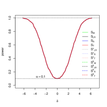
(a) normal

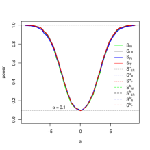
(b) Student-t with $\nu=4$

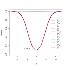
(c) type II logistic

Figure 1: Power of the tests for $n=30$, $p=4$, $q=3$, $\phi=3$, and $\alpha=10\%$.

Overall, the Monte Carlo simulation results reveal that, in small and moderate-sized samples, the Wald, likelihood ratio, score and gradient tests tend to be liberal, i.e. they wrongly reject the null hypothesis more frequently than allowed by the chosen nominal significance level. Among all the tests we considered, the Wald test is clearly the most liberal. The Bartlett and Bartlett-type corrections are effective in correcting the size distortions of the tests with virtually no power loss. The bootstrapped tests perform similarly to the analytically corrected tests at the cost of requiring computationally-intensive calculations. There is no Bartlett-type correction available to the Wald statistic and, hence, the bootstrap method is a convenient tool to correct its liberal behavior. We conclude that the modified (analytically corrected or bootstrapped) tests are to be preferred for testing hypotheses in symmetric and log-symmetric linear regression models when the sample is small or of moderate size.

6 Applications

We now present applications of all the tests in two data sets to illustrate the need for corrections in small samples. First, we deal with the data set presented in Nateghi et al. (2012). The aim is to investigate the effect of fat replacers on texture properties of Cheddar cheeses. Here, the response variable is the cohesiveness ($t_{l}$) of the cheese and the covariates are the percentage of fat ($x_{1}=1.25\%$ – low-fat cheese, and $2.00\%$ – reduced-fat cheese), percentage of xanthan gum ($x_{2l}=0.030\%$ and $0.045\%$), and percentage of sodium caseinate ($x_{3l}=0.00\%$ and $0.15\%$). Observations were taken in $n=16$ samples of cheese in a full factorial design with two replicates; see Tables 1 and 6 in Nateghi et al. (2012). We fit the following log-symmetric linear regression model

$$\log(t_{l})=\beta_{0}+\beta_{1}x_{1l}+\beta_{2}x_{2l}+\beta_{3}x_{3l}+\beta_{4}x_{1l}x_{2l}+\beta_{5}x_{1l}x_{3l}+\beta_{6}x_{2l}x_{3l}+\phi\epsilon_{l},$$ (10)

for $l=1,\ldots,16$, where $\epsilon_{l}\sim S(0,1)$ are independent random errors. We considered the following standard symmetric distributions for the errors: normal, Student-t with different values for the degrees of freedom parameter, and type II logistic. The corrected AIC criteria (Burnham and Anderson, 2004) for the fitted models are: $-135.25$ (normal), $-134.87$ (Student-t with $\nu=3$), $-135.02$ (Student-t with $\nu=4$), $-135.03$ (Student-t with $\nu=5$), and $-134.98$ (type II log-logistic). The smallest AIC is achieved by the log-normal model. Among the log-Student-t models the smallest AIC corresponds to $\nu=5$. Figure 2 shows the normal quantile-quantile plot with simulated enveloped for the standardized residuals proposed by Villegas et al. (2013) for the log-normal model, log-Student-t model with $\nu=5$, and type II log-logistic model. Figure 2 and the AIC criteria suggest that the model that best fits the data is the log-normal linear regression model. This is the model chosen for the analysis that follow. The maximum likelihood estimates of the parameters (standard errors in parentheses) are: $\widehat{\beta}_{0}=-0.1321\,(0.0067)$, $\widehat{\beta}_{1}=-0.0043\,(0.0039)$, $\widehat{\beta}_{2}=-0.1456\,(0.1712)$, $\widehat{\beta}_{3}=0.0135\,(0.0251)$, $\widehat{\beta_{4}}=-0.1864\,(0.1001)$, $\widehat{\beta_{5}}=-0.0074\,(0.0100)$, $\widehat{\beta_{6}}=0.6606\,(0.5007)$, and $\widehat{\phi}=0.0011\,(0.0002)$.

(a) log-normal

(b) log-Student-t

(c) type II log-logistic

Figure 2: Normal quantile-quantile plots of standardized residuals for model (10): log-normal model (a), log-Student-t model (b), and type II log-logistic model (c); Cheddar cheese data.

We first test each interaction effect, i.e. the null hypotheses of interest are ${\cal H}_{0}:\beta_{4}=0$, ${\cal H}_{0}:\beta_{5}=0$, and ${\cal H}_{0}:\beta_{6}=0$. The test statistics ($p$-values in parentheses) for testing ${\cal H}_{0}:\beta_{4}=0$ are: $S_{\textrm{W}}=3.4632$ (0.0628), $S_{\textrm{LR}}=3.1350$ (0.0766), $S_{\textrm{R}}=2.8470$ (0.0915), $S_{\textrm{T}}=2.8469$ (0.0915), $S_{\textrm{LR}}^{*}=1.6654$ (0.1969), $S_{\textrm{R}}^{*}=1.7657$ (0.1839), and $S_{\textrm{T}}^{*}=1.7657$ (0.1839). The $p$-values for all the bootstrapped tests are $0.2036$. Note that the $p$-values vary from $6.3\%$ to $20.4\%$. Although none of the tests reject the null hypothesis at the $10\%$ nominal level, at the $5\%$ nominal level the uncorrected tests lead to rejection of ${\cal H}_{0}$ unlike the analytically corrected and bootstrapped tests. As evidenced by our simulations, the uncorrected tests tend to be liberal in small samples (recall that $n=16$), and the modified tests are less size distorted. The null hypotheses ${\cal H}_{0}:\beta_{5}=0$ and ${\cal H}_{0}:\beta_{6}=0$ are not rejected by none of the tests for all the usual significance levels (all the $p$-values are greater than 45% and 18% for the test of ${\cal H}_{0}:\beta_{5}=0$ and ${\cal H}_{0}:\beta_{6}=0$, respectively). We now test the hypothesis of no joint interactions effect, i.e. ${\cal H}_{0}:\beta_{4}=\beta_{5}=\beta_{6}=0$. None of the tests rejects ${\cal H}_{0}$ at the usual significance levels (all the $p$-values are greater than 12%).

We now remove the interaction effects in model (10) and estimate the model

$$\log(t_{l}) =\beta_{0}+\beta_{1}x_{1l}+\beta_{2}x_{2l}+\beta_{3}x_{3l}+\phi\epsilon_{l},\qquad l=1,\ldots,16.$$ (11)

The maximum likelihood estimates (asymptotic standard errors in parentheses) are: $\widehat{\beta_{0}}=-0.1217\,$ $(0.0022)$, $\widehat{\beta_{1}}=-0.0119\,(0.0009)$, $\widehat{\beta_{2}}=-0.3989\,(0.0438)$, $\widehat{\beta_{3}}=0.0262\,(0.0044)$, and $\widehat{\phi}=0.0013\,$ $(0.0002)$. The null hypotheses ${\cal H}_{0}:\beta_{1}=0$, ${\cal H}_{0}:\beta_{2}=0$, and ${\cal H}_{0}:\beta_{3}=0$ are strongly rejected by all the tests at the usual significance levels. Figure 3 shows the normal quantile-quantile plot of the standardized residuals for model (11). The plot suggests a reasonable fit. Hence, the final estimated model for the median cohesiveness of the low-fat and reduced-fat Cheddar cheese is

$$\widehat{\eta}=e^{-0.1217-0.0119x_{1}-0.3989x_{2}+0.0262x_{3}}.$$

Figure 3: Normal quantile-quantile plot of standardized residuals for model (11); Cheddar cheese data.

The second application considers the data set presented in Table 1 of Mirhosseini and Tan (2010). The data were collected to investigate the effect of emulsion components on orange beverage emulsion properties. The independent variables are the amount of gum arabic ($x_{1}$), xanthan gum ($x_{2}$) and orange oil ($x_{3}$), all measured in $g/100g$, and the response variable is the emulsion density ($y$) measured in $g/cm^{3}$. We fitted the following regression model

$$y_{l}=\beta_{0}+\beta_{1}x_{1l}+\beta_{2}x_{2l}+\beta_{3}x_{3l}+\beta_{4}x_{1l}x_{2l}+\beta_{5}x_{1l}x_{3l}+\beta_{6}x_{2l}x_{3l}+\phi\epsilon_{l},$$ (12)

for $l=1,\ldots,20$, where $\epsilon_{l}\sim S(0,1)$ are independent errors. Different choices of the error distribution were considered as in the first application. The corrected AIC for the fitted models are: $-150.03$ (normal), $-158.68$ (Student-t with $\nu=3$), $-156.37$ (Student-t with $\nu=4$), $-154.48$ (Student-t with $\nu=5$), and $-151.03$ (type II logistic). Normal quantile-quantile plots of standardized residuals (not shown) and the corrected AICs point to the Student-t model with $\nu=3$ as the best model. The maximum likelihood estimates of the parameters (asymptotic standard errors in parentheses) are: $\widehat{\beta}_{0}=0.9388\,(0.0220)$, $\widehat{\beta}_{1}=0.0054\,(0.0011)$, $\widehat{\beta}_{2}=0.1563\,(0.0401)$, $\widehat{\beta}_{3}=0.0016\,(0.0016)$, $\widehat{\beta}_{4}=-0.0048\,(0.0015)$, $\widehat{\beta}_{5}=-0.0001\,(0.0001)$, $\widehat{\beta}_{6}=-0.0070\,(0.0026)$, and $\widehat{\phi}=0.0012\,(0.0003)$.

We first test the individual interaction effects, i.e. the null hypotheses under test are ${\cal H}_{0}:\beta_{4}=0$, ${\cal H}_{0}:\beta_{5}=0$, and ${\cal H}_{0}:\beta_{6}=0$; see Table 8 for the test statistics and $p$-values. The null hypothesis ${\cal H}_{0}:\beta_{4}=0$ is rejected by the Wald, likelihood ratio and gradient tests at the $5\%$ nominal level. However, the opposite decision is reached by the score and the modified tests. None of the tests reject ${\cal H}_{0}:\beta_{5}=0$, and ${\cal H}_{0}:\beta_{6}=0$ is rejected by the Wald and likelihood ratio tests at the $5\%$ nominal level, but is not rejected by the others. It is noticeable that there is no conflict among the modified tests, and all of them do not show enough evidence to reject the null hypotheses. We then test the joint interactions effect in model (12), i.e. the null hypothesis is ${\cal H}_{0}:\beta_{4}=\beta_{5}=\beta_{6}=0$. The test statistics ($p$-values in parentheses) are: $S_{\textrm{W}}=17.9297$ (0.0005), $S_{\textrm{LR}}=8.1531$ (0.0430), $S_{\textrm{R}}=2.9646$ (0.3971), $S_{\textrm{T}}=4.5884$ (0.2045), $S_{\textrm{LR}}^{*}=4.0333$ (0.2579), $S_{\textrm{R}}^{*}=2.1259$ (0.5467), and $S_{\textrm{T}}^{*}=3.1251$ (0.3727). The $p$-values of the bootstrapped Wald, likelihood ratio, score and gradient tests are $0.1838$, $0.2280$, $0.5868$, and $0.3466$, respectively. Note that the $p$-values range from $0.05\%$ (Wald) to $58.7\%$ (bootstrapped score test). While the Wald and the likelihood ratio tests reject the joint interactions effect, the other tests point to the opposite direction.

Table 8: Test statistics and $p$-values for testing ${\cal H}_{0}:\beta_{4}=0$, ${\cal H}_{0}:\beta_{5}=0$, and ${\cal H}_{0}:\beta_{6}=0$ in model (12); orange emulsion data.

	${\cal H}_{0}:\beta_{4}=0$		${\cal H}_{0}:\beta_{5}=0$		${\cal H}_{0}:\beta_{6}=0$
statistic	observed value	$p-$value	observed value	$p-$value	observed value	$p-$value
${S}_{\textrm{W}}$	10.2240	0.0014	0.4583	0.4984	7.2474	0.0071
${S}_{{\textrm{LR}}}$	6.5050	0.0108	0.5354	0.4644	5.2526	0.0219
${S}_{{\textrm{R}}}$	3.5812	0.0584	0.6040	0.4371	3.3333	0.0679
${S}_{{\textrm{T}}}$	4.1713	0.0411	0.5148	0.4731	3.5959	0.0579
${S}^{*}_{{\textrm{LR}}}$	2.5065	0.1134	0.2063	0.6497	2.0239	0.1548
${S}^{*}_{{\textrm{R}}}$	2.2753	0.1314	0.3500	0.5541	2.1023	0.1471
${S}^{*}_{{\textrm{T}}}$	2.1510	0.1425	0.2066	0.6494	1.7897	0.1810
${S}^{b}_{{\textrm{W}}}$		0.1054		0.6728		0.1532
${S}^{b}_{{\textrm{LR}}}$		0.0930		0.6242		0.1266
${S}^{b}_{{\textrm{R}}}$		0.1562		0.5506		0.1690
${S}^{b}_{{\textrm{T}}}$		0.1318		0.6194		0.1650

Removing the interaction effects in (12) we now estimate the model

$$\begin{split}y_{l}&=\beta_{0}+\beta_{1}x_{1l}+\beta_{2}x_{2l}+\beta_{3}x_{3l}+\phi\epsilon_{l}.\end{split}$$ (13)

The maximum likelihood estimates (asymptotic standard errors in parentheses) are $\widehat{\beta_{0}}=1.0198\,$ $(0.0051)$, $\widehat{\beta_{1}}=0.0027\,(0.0002)$, $\widehat{\beta_{2}}=-0.0058\,(0.0059)$, $\widehat{\beta_{3}}=-0.0023\,(0.0003)$, and $\widehat{\phi}=0.0018\,$ $(0.0004)$. At the usual nominal significance levels, all the tests strongly reject ${\cal H}_{0}:\beta_{1}=0$ and ${\cal H}_{0}:\beta_{3}=0$. Also, all the tests suggest the removal of $x_{2}$ from model (13). Hence, the final model is $y_{l}=\beta_{0}+\beta_{1}x_{1l}+\beta_{3}x_{3l}+\phi\epsilon_{l}.$ The maximum likelihood estimates of the parameters are $\widehat{\beta}_{0}=1.0168\,(0.0047)$, $\widehat{\beta}_{1}=0.0027\,(0.0002)$, $\widehat{\beta}_{3}=-0.0023\,(0.0003)$, and $\widehat{\phi}=0.0018\,(0.0004)$. The normal quantile-quantile plot of standardized residuals for the final estimated model (not shown) suggests a suitable fit.

7 Final remarks

This paper dealt with the issue of testing hypotheses in symmetric and log-symmetric linear regression models. The models can be easily fitted using the available package ssym in R. Testing inference using the classic tests and the recently proposed gradient test rely on asymptotic approximations and may be unreliable when the sample size is small or even moderate. Our simulations indicate that the Wald and the likelihood tests may be severely liberal in finite samples. The score and the gradient tests are less size distorted but may present considerable size distortion depending on the number of observations, regression parameters, and parameters under test.

We derived a Bartlett-type correction to the gradient statistic in symmetric linear regression models. We showed that this correction and the corrections to the likelihood ratio and score statistics found in the literature are also valid for log-symmetric linear regression models. We then performed simulation experiments comparing the uncorrected tests and their corresponding analytically corrected (except for the Wald test) and bootstrapped versions. The simulations are clear in indicating that the modified tests are much less size distorted than the original tests and that all the tests have similar power. The analytical corrections are simple and easily implemented is any software that performs matrix computation, such as R. The bootstrapped tests, on the other hand, requires computationally-intensive calculations. Since there is no Bartlett-type correction available to the Wald statistic, the bootstrap method is convenient when performing Wald tests.

We presented two applications for real data. Our analyses illustrate that the use of the original tests may be misleading in small samples. The usefulness of the analytically corrected and bootstrapped tests became clear. We, therefore, recommend the use of the modified tests when performing testing inference in symmetric and log-symmetric linear regression models.

Appendix

Let $\kappa_{rs}={\rm E}(\partial^{2}\ell/\partial\beta_{r}\partial\beta_{s})$, $\kappa_{rst}={\rm E}(\partial^{3}\ell/\partial\beta_{r}\partial\beta_{s}\partial\beta_{t})$, $\kappa_{rstu}={\rm E}(\partial^{4}\ell/\partial\beta_{r}\partial\beta_{s}\partial\beta_{t}\partial\beta_{u})$, $\kappa_{rs}^{(t)}=\partial\kappa_{rs}/\partial\beta_{t}$, $\kappa_{rs}^{(tu)}=\partial^{2}\kappa_{rs}/\partial\beta_{t}\partial\beta_{u}$, $\kappa_{\phi\phi}={\rm E}(\partial^{2}\ell/\partial\phi^{2})$, $\kappa_{r\phi}={\rm E}(\partial^{2}\ell/\partial\beta_{r}\partial\phi)$, $\kappa_{r\phi}^{(s)}=\partial^{2}\kappa_{r\phi}/\partial\beta_{s}$ and so on. The indices $r$, $s$, $t$ and $u$ vary from $1$ to $p$. In symmetric linear regression models we have

$$\kappa_{rs} =\frac{\delta_{01000}}{\phi^{2}}\sum_{l=1}^{n}x_{lr}x_{ls},\qquad\kappa_{rstu}=\frac{\delta_{00010}}{\phi^{4}}\sum_{l=1}^{n}x_{lr}x_{ls}x_{lu}x_{lt},\qquad\kappa_{rst}=\kappa_{rs}^{(t)}=\kappa_{rst}^{(u)}=\kappa_{rs}^{(tu)}=0,$$

$$\kappa_{\phi\phi} =-\frac{n}{\phi^{2}}(1-\delta_{20002}),\qquad\kappa^{(\phi)}_{\phi\phi}=-\frac{2n}{\phi^{3}}(\delta_{01002}-1),\qquad\kappa_{\phi\phi\phi}=-\frac{n}{\phi^{3}}(6\delta_{01002}+\delta_{00103}-4),$$

$$\kappa_{r\phi} =\kappa_{r\phi}^{(s)}=\kappa_{r\phi\phi}=\kappa^{(u)}_{r\phi\phi}=0,\qquad\kappa_{rs\phi}=-\frac{1}{\phi^{3}}(\delta_{00101}+2\delta_{01000})\sum_{l=1}^{n}x_{lr}x_{ls},$$

$$\kappa_{rs\phi\phi} =-\frac{1}{\phi^{4}}(\delta_{00012}-6\delta_{11001})\sum_{l=1}^{n}x_{lr}x_{ls},\qquad\kappa^{(\phi)}_{rs\phi}=\frac{3}{\phi^{4}}(\delta_{00101}+2\delta_{01000})\sum_{l=1}^{n}x_{lr}x_{ls},$$

$$\kappa^{(\phi)}_{rs} =-\frac{2\delta_{01000}}{\phi^{3}}\sum_{l=1}^{n}x_{lr}x_{ls},$$

see Ferrari and Uribe-Opazo (2001) and Uribe-Opazo et al. (2008).

Let $\bm{K}^{-1}={\rm diag}\{\bm{K}^{-1}_{\bm{\beta}},-\kappa^{-1}_{\phi\phi}\}$ be the Fisher information matrix inverse of $(\bm{\beta}_{1}^{\top},\bm{\beta}_{2}^{\top},\phi)^{\top}$. Let

$${\bm{\mathcal{A}}}_{\bm{\beta}}=\begin{bmatrix}\bm{0}&\bm{0}\\ \bm{0}&\bm{K}_{\bm{\beta}_{22}}^{-1}\end{bmatrix},\qquad{\bm{\mathcal{M}}}_{\bm{\beta}}=\bm{K}^{-1}_{\bm{\beta}}-{\bm{\mathcal{A}}}_{\bm{\beta}},$$

${\bm{\mathcal{A}}}_{\bm{\beta}\phi}={\rm diag}\{{\bm{\mathcal{A}}}_{\bm{\beta}},-\kappa^{-1}_{\phi\phi}\}$, and ${\bm{\mathcal{M}}}_{\bm{\beta}\phi}={\rm diag}\{{\bm{\mathcal{M}}}_{\bm{\beta}},0\}$. We denote by $m^{r\phi}$ and $a^{r\phi}$ the element $(r,p+1)$ of $\bm{\mathcal{M}}_{\bm{\beta}\phi}$ and $\bm{\mathcal{A}}_{\bm{\beta}\phi}$, respectively. Analogously, $m^{\phi\phi}$ and $a^{\phi\phi}$ represent the element $(p+1,p+1)$ of $\bm{\mathcal{M}}_{\bm{\beta}\phi}$ and $\bm{\mathcal{A}}_{\bm{\beta}\phi}$, respectively. We have $m^{r\phi}=m^{\phi r}=m^{\phi\phi}=a^{r\phi}=a^{\phi r}=0$, for $r=1,\ldots,p$, and $a^{\phi\phi}=-\kappa_{\phi\phi}^{-1}$.

The coefficients $A_{{\textrm{T}}}$’s that define the Bartlett-type correction to the gradient statistic in symmetric linear regression models are obtained by replacing the moments above in the formulas for the $A$’s in Theorem 1 of Vargas et al. (2013). We first note that $A_{{\textrm{T}}11}=A_{{\textrm{T}}1}+A_{{\textrm{T}}1,\bm{\beta}\phi}$, $A_{{\textrm{T}}22}=A_{{\textrm{T}}2}+A_{{\textrm{T}}2,\bm{\beta}\phi}$, and $A_{{\textrm{T}}33}=A_{{\textrm{T}}3}+A_{{\textrm{T}}3,\bm{\beta}\phi}$, where $A_{{\textrm{T}}1}$, $A_{{\textrm{T}}2}$, and $A_{{\textrm{T}}3}$ are the coefficients obtained assuming that $\phi$ is known and $A_{{\textrm{T}}1,\bm{\beta}\phi}$, $A_{{\textrm{T}}2,\bm{\beta}\phi}$, and $A_{{\textrm{T}}3,\bm{\beta}\phi}$ are the additional terms that appear when $\phi$ is unknown.

By replacing the moments above in the formula of $A_{1}$ in Theorem 1 of Vargas et al. (2013), the coefficient $A_{{\textrm{T}}1}$ can be written as

$${A}_{{\textrm{T}}1}=6\sum\nolimits^{\prime}\kappa_{jrsu}m^{jr}a^{su}=\frac{6\delta_{00010}}{\phi^{4}}\sum\nolimits^{\prime}\sum_{l=1}^{n}x_{lr}x_{lj}x_{ls}x_{lu}m^{jr}a^{su},$$

where $\sum\nolimits^{\prime}$ is the summation over the indices of the parameter $\bm{\beta}$. Inverting the order of the summations and rearranging the terms we have

$${A}_{{\textrm{T}}1}=\frac{6\delta_{00010}}{\phi^{4}}\sum_{l=1}^{n}\left(\sum\nolimits^{\prime}x_{lj}m^{jr}x_{lr}\right)\left(\sum\nolimits^{\prime}x_{ls}a^{su}x_{lu}\right).$$

The terms $\sum\nolimits^{\prime}x_{li}a^{ij}x_{lj}$ and $\sum\nolimits^{\prime}x_{li}m^{ij}x_{lj}$ represent the $(l,l)$ element of the matrices $\phi^{2}\bm{Z}_{2}/\delta_{20000}$ and $\phi^{2}(\bm{Z}-\bm{Z}_{2})/\delta_{20000}$, respectively. Hence,

$${A}_{{\textrm{T}}1}==\frac{6\delta_{00010}}{\delta^{2}_{20000}}\sum_{l=1}^{n}(z_{ll}-z_{2ll})z_{2ll}=\frac{6c_{0}}{n}(\rho_{ZZ_{2}}-\rho_{Z_{2}Z_{2}}),$$

where $c_{0}$ and the $\rho$’s are given in Section 4.

Analogously, we have

$${A}_{{\textrm{T}}2} =-3\sum\nolimits^{\prime}\kappa_{jrsu}m^{jr}m^{su}=-\frac{3\delta_{00010}}{\phi^{4}}\sum_{l=1}^{n}\left(\sum\nolimits^{\prime}x_{lj}m^{jr}x_{lr}\right)\left(\sum\nolimits^{\prime}x_{ls}m^{su}x_{lu}\right)$$

$$=-\frac{3\delta_{00010}}{\delta^{2}_{20000}}\sum_{l=1}^{n}(z_{ll}-z_{2ll})^{2}=-\frac{3c_{0}}{n}(\rho_{ZZ}-2\rho_{ZZ_{2}}+\rho_{Z_{2}Z_{2}})$$

and ${A}_{{\textrm{T}}3}=0.$

We now turn to the derivation of $A_{{\textrm{T}}1,\bm{\beta}\phi}$, $A_{{\textrm{T}}2,\bm{\beta}\phi}$, and $A_{{\textrm{T}}3,\bm{\beta}\phi}$. These terms only appear when $\phi$ is unknown. When $\phi$ is unknown, which is usually the case, it follows from Theorem 1 of Vargas et al. (2013) that $A_{{\textrm{T}}3,\bm{\beta}\phi}=0$,

$$\begin{split}{A}_{{\textrm{T}}1,\bm{\beta}\phi}&=\sum\nolimits^{\prime}\kappa_{jrs}\kappa_{u\phi\phi}a^{\phi\phi}m^{jr}m^{su}+\sum\nolimits^{\prime}\kappa_{jrs}\kappa_{u\phi\phi}a^{\phi\phi}m^{js}m^{ru}\\ &\quad+\sum\nolimits^{\prime}\kappa_{jrs}\kappa_{u\phi\phi}a^{\phi\phi}m^{ju}m^{rs}+6\sum\nolimits^{\prime}\kappa_{jr\phi}\kappa_{\phi\phi\phi}m^{jr}(a^{\phi\phi})^{2}\\ &\quad+6\sum\nolimits^{\prime}\kappa_{jr\phi}\kappa_{vw\phi}m^{jr}a^{vw}a^{\phi\phi}+6\sum\nolimits^{\prime}\kappa_{jrs}\kappa_{u\phi\phi}m^{jr}a^{su}a^{\phi\phi}\\ &\quad+3\sum\nolimits^{\prime}\kappa_{j\phi\phi}\kappa_{uvw}m^{ju}a^{vw}a^{\phi\phi}+3\sum\nolimits^{\prime}\kappa_{jrs}\kappa_{u\phi\phi}m^{ju}a^{rs}a^{\phi\phi}\\ &\quad+3\sum\nolimits^{\prime}\kappa_{j\phi\phi}\kappa_{u\phi\phi}m^{ju}(a^{\phi\phi})^{2}+3\sum\nolimits^{\prime}\kappa_{jr\phi}\kappa_{uw\phi}m^{ju}a^{rw}a^{\phi\phi}\\ &\quad+3\sum\nolimits^{\prime}\kappa_{js\phi}\kappa_{uv\phi}m^{ju}a^{sv}a^{\phi\phi}+3\sum\nolimits^{\prime}\kappa_{jr\phi}\kappa_{uv\phi}m^{ju}a^{rv}a^{\phi\phi}\\ &\quad+3\sum\nolimits^{\prime}\kappa_{js\phi}\kappa_{uw\phi}m^{ju}a^{sw}a^{\phi\phi}-6\sum\nolimits^{\prime}(\kappa_{jr\phi}^{(\phi)}-\kappa_{jr\phi\phi})m^{jr}a^{\phi\phi}\\ &\quad-6\sum\nolimits^{\prime}\kappa_{jr\phi}^{(\phi)}m^{jr}a^{\phi\phi}-12\sum\nolimits^{\prime}\kappa_{j\phi\phi}^{(u)}m^{ju}a^{\phi\phi}\\ &\quad-12\sum\nolimits^{\prime}\kappa_{kl}^{(\phi)}\kappa_{jr\phi}(\kappa^{jk}\kappa^{lr}-a^{jk}a^{lr})a^{\phi\phi}-12\sum\nolimits^{\prime}\kappa_{\phi\phi}^{(\phi)}\kappa_{jr\phi}m^{jr}(a^{\phi\phi})^{2}\\ &\quad-12\sum\nolimits^{\prime}\kappa_{j\phi\phi}\kappa_{kl}^{(u)}(\kappa^{jk}\kappa^{lu}-a^{jk}a^{lu})a^{\phi\phi},\end{split}$$ (14)

and

$$\begin{split}{A}_{{\textrm{T}}2,\bm{\beta}\phi}&=-\sum\nolimits^{\prime}\kappa_{jrs}\kappa_{u\phi\phi}m^{jr}m^{su}a^{\phi\phi}-\sum\nolimits^{\prime}\kappa_{jrs}\kappa_{u\phi\phi}m^{js}m^{ru}a^{\phi\phi}\\ &\quad-\sum\nolimits^{\prime}\kappa_{jrs}\kappa_{u\phi\phi}m^{ju}m^{rs}a^{\phi\phi}-3\sum\nolimits^{\prime}\kappa_{jr\phi}\kappa_{uv\phi}m^{jr}m^{uv}a^{\phi\phi}\\ &\quad-3\sum\nolimits^{\prime}\kappa_{jr\phi}\kappa_{uv\phi}m^{ju}m^{rv}a^{\phi\phi}-3\sum\nolimits^{\prime}\kappa_{jr\phi}\kappa_{uv\phi}m^{jv}m^{ru}a^{\phi\phi}.\end{split}$$ (15)

Plugging the $\kappa$’s in (14) and (15) some terms vanish. By inverting the summation order and rearranging the terms we have

$$\begin{split}{A}_{{\textrm{T}}1,\bm{\beta}\phi}&=\frac{6(\delta_{00101}+2\delta_{01000})(6\delta_{01002}+\delta_{00103}-4)}{n\phi^{2}(\delta_{20002}-1)^{2}}\sum_{l=1}^{n}\left(\sum\nolimits^{\prime}x_{lj}m^{jr}x_{lr}\right)\\ &+\frac{6(\delta_{00101}+2\delta_{01000})^{2}}{n\phi^{4}(\delta_{20002}-1)}\sum_{l,i=1}^{n}\left(\sum\nolimits^{\prime}x_{lj}m^{jr}x_{lr}\right)\left(\sum\nolimits^{\prime}x_{iv}a^{vw}x_{iw}\right)\\ &-\frac{36(\delta_{00101}+2\delta_{01000})}{n\phi^{2}(\delta_{20002}-1)}\sum_{l=1}^{n}\left(\sum\nolimits^{\prime}x_{lj}m^{jr}x_{lr}\right)+\frac{6(\delta_{00012}-6\delta_{11001})}{n\phi^{2}(\delta_{20002}-1)}\sum_{l=1}^{n}\left(\sum\nolimits^{\prime}x_{lj}m^{jr}x_{lr}\right)\\ &-\frac{24\delta_{01000}(\delta_{00101}+2\delta_{01000})}{n\phi^{4}(\delta_{20002}-1)}\sum_{l=1}^{n}\left(-\sum\nolimits^{\prime}x_{lj}k^{jk}x_{ik}\right)\left(-\sum\nolimits^{\prime}x_{is}k^{sr}x_{lr}\right)\\ &+\frac{24\delta_{01000}(\delta_{00101}+2\delta_{01000})}{n\phi^{4}(\delta_{20002}-1)}\sum_{l=1}^{n}\left(\sum\nolimits^{\prime}x_{lj}a^{jk}x_{ik}\right)\left(\sum\nolimits^{\prime}x_{is}a^{sr}x_{lr}\right)\\ &-\frac{24(\delta_{01002}-1)(\delta_{00101}+2\delta_{01000})}{n\phi^{2}(\delta_{20002}-1)^{2}}\sum_{l=1}^{n}\left(\sum\nolimits^{\prime}x_{lj}m^{jr}x_{lr}\right)\end{split}$$

and

$$\begin{split}{A}_{{\textrm{T}}2,\bm{\beta}\phi}&=-\frac{3(\delta_{00101}+2\delta_{01000})^{2}}{n\phi^{4}(\delta_{20002}-1)}\sum_{l,i=1}^{n}\left(\sum\nolimits^{\prime}x_{lj}m^{jr}x_{lr}\right)\left(\sum\nolimits^{\prime}x_{iu}m^{uv}x_{iv}\right)\\ &-\frac{6(\delta_{00101}+2\delta_{01000})^{2}}{n\phi^{4}(\delta_{20002}-1)}\sum_{l,i=1}^{n}\left(\sum\nolimits^{\prime}x_{lj}m^{ju}x_{iu}\right)\left(\sum\nolimits^{\prime}x_{lr}a^{rv}x_{iv}\right).\\ \end{split}$$

Note that $\sum\nolimits^{\prime}x_{li}\kappa^{ij}x_{lj}$ equals the $(l,l)$ element of the matrix $\phi^{2}\bm{Z}/\delta_{20000}$ and that

$$\qquad\sum\nolimits^{\prime}z_{ll}=\mathrm{tr}(Z_{d})=p,\qquad\sum\nolimits^{\prime}z_{2ll}=\mathrm{tr}(Z_{2d})=p-q,\qquad\sum\nolimits^{\prime}(z_{ll}-z_{2ll})=\mathrm{tr}(Z_{d}-Z_{2d})=q.$$

Hence,

$$\begin{split}{A}_{{\textrm{T}}1,\bm{\beta}\phi}&=\frac{6(\delta_{00101}+2\delta_{01000})(6\delta_{01002}+\delta_{00103}-4)}{n\delta_{20000}(\delta_{20002}-1)^{2}}q+\frac{6(\delta_{00101}+2\delta_{01000})^{2}}{n\delta^{2}_{20000}(\delta_{20002}-1)}q(p-q)\\ \\ &-\frac{36(\delta_{00101}+2\delta_{01000})}{\delta_{20000}(\delta_{20002}-1)}q+\frac{6(\delta_{00012}-6\delta_{11001})}{n\delta_{20000}(\delta_{20002}-1)}q-\frac{24\delta_{01000}(\delta_{00101}+2\delta_{01000})}{n\delta^{2}_{20000}(\delta_{20002}-1)}p\\ \\ &+\frac{24\delta_{01000}(\delta_{00101}+2\delta_{01000})}{n\delta^{2}_{20000}(\delta_{20002}-1)}(p-q)-\frac{24(\delta_{01002}-1)(\delta_{00101}+2\delta_{01000})}{n\delta^{2}_{20000}(\delta_{20002}-1)^{2}}q\end{split}$$

and

$$\begin{split}{A}_{{\textrm{T}}2,\bm{\beta}\phi}&=-\frac{3(\delta_{00101}+2\delta_{01000})^{2}}{n\delta^{2}_{20000}(\delta_{20002}-1)}\left(q^{2}+2q\right).\end{split}$$

After some algebra, we arrive at the expressions for ${A}_{{\textrm{T}}1,\bm{\beta}\phi}$ and ${A}_{{\textrm{T}}2,\bm{\beta}\phi}$ given in Section 4.

References

• Andrews and Mallows (1974) Andrews D.R, Mallows C.L. (1974). Scale mixtures of normal distributions. Journal of the Royal Statistical Society B, 36, 99–102.
• Barroso and Cordeiro (2005) Barroso, L.P., Cordeiro, G.M. (2005). Bartlett corrections in heteroskedastic t regression models. Statistics & Probability Letters 75, 86–96.
• Bartlett (1937) Bartlett, M.S. (1937). Properties of sufficiency and statistical tests. Proceedings of the Royal Society A 160, 268–282.
• Bayer and Cribari-Neto (2013) Bayer, F.M., Cribari-Neto, F. (2013). Bartlett corrections in beta regression models. Journal of Statistical Planning and Inference 143, 531–547.
• Berkane and Bentler (1986) Berkane, M., Bentler, P.M. (1986). Moments of elliptically distributed random variates. Statistics & Probability Letters 4, 333–335.
• Burnham and Anderson (2004) Burnham, K.P., Anderson, D.R. (2004). Multimodel inference: understanding AIC and BIC in model selection. Sociological methods $\&$ research 33, 261–304.
• Chan et al. (2014) Chan, H., Chen, K., Yau, C.Y. (2014). On the Bartlett correction of empirical likelihood for Gaussian long-memory time series. Electronic Journal of Statistics 8, 1460–1490.
• Cordeiro (2004) Cordeiro, G.M. (2004). Corrected likelihood ratio tests in symmetric nonlinear regression models. Journal of Statistical Computation and Simulation 74, 609–620.
• Cordeiro and Ferrari (1991) Cordeiro, G.M., Ferrari, S.L.P. (1991). A modified score test statistic having chi-squared distribution to order $n^{-1}$. Biometrika 78, 573–582.
• Cox and Hinkley (1974) Cox, D.R., Hinkley, D.V., (1974). Theoretical Statistics. Chapman and Hall, London
• Cysneiros et al. (2007) Cysneiros, J.F.A., Paula, G.A., Galea, M. (2007). Heteroscedastic symmetrical linear models. Statistics & Probability Letters 77, 1084–1090.
• Cysneiros et al. (2010) Cysneiros, A.H.M.A., Rodrigues, K.S.P., Cordeiro, G.M., Ferrari, S.L.P. (2010). Three Bartlett-type corrections for score statistics in symmetric nonlinear regression models. Statistical Papers 51, 273–284.
• da Silva and Cordeiro (2009) da Silva, D.N., Cordeiro, G.M. (2009). A computer program to improve LR tests for generalized linear models. Communications in Statistics 38, 2184–2197.
• da Silva-Júnior et al. (2014) da Silva-Júnior, A.H.M., da Silva, D.N., Ferrari, S.L.P. (2014). mdscore: An R package to compute improved score tests in generalized linear models. Journal of Statistical Software 61, 1–16, url: http://www.jstatsoft.org/v61/c02/.
• Dempster et al. (1977) Dempster, A.P., Laird, N.M., Rubin, D.B. (1977). Maximum likelihood from incomplete data via the EM algorithm. Journal of the Royal Statistical Society B 39, 1–38.
• Doornik (2013) Doornik, J.A. (2013). Object-Oriented Matrix Programming Using Ox. Timberlake Consultants Press, London.
• Efron and Tibshirani (1993) Efron, B., Tibshirani, R.J. (1993). An Introduction to the Bootstrap, Chapman & Hall, New York.
• Fang et al. (1990) Fang, K., Kotz, S., Ng, K. (1990). Symmetric Multivariate and Related Distribution. Chapman & Hall, London.
• Ferrari and Uribe-Opazo (2001) Ferrari, S.L.P., Uribe-Opazo, M.A. (2001). Corrected likelihood ratio tests in a class of symmetric linear regression models. Brazilian Journal of Probability and Statistics 15, 49–67.
• Galea et al. (2005) Galea, M., Paula, G.A., Cysneiros, F.J.A. (2005). On diagnostics in symmetrical nonlinear models. Statistics and Probability Letters 73, 459–467.
• Lagos et al. (2010) Lagos, B.M., Morettin, P.A., Barroso, L.P. (2010). Some corrections of the score test statistic for Gaussian ARMA models. Brazilian Journal of Probability and Statistics 24, 434–456.
• Lawley (1956) Lawley, D. (1956). A general method for approximating to the distribution of likelihood ratio criteria. Biometrika 43, 295–303.
• Lemonte et al. (2010) Lemonte, A.J., Ferrari, S.L.P., Cribari–Neto, F. (2010). Improved likelihood inference in Birnbaum–Saunders regressions. Computational Statistics & Data Analysis 54, 1307–1316.
• Lemonte and Ferrari (2011) Lemonte, A.J., Ferrari, S.L.P. (2011). Small-sample corrections for score tests in Birnbaum–Saunders regressions. Communications in Statistics – Theory and Methods 40, 232–243.
• Lemonte (2012) Lemonte, A.J. (2012). Local power properties of some asymptotic tests in symmetric linear regression models. Journal of Statistical Planning and Inference 142, 1178–1188.
• Lemonte and Ferrari (2012) Lemonte, A.J., Ferrari, S.L.P. (2012). The local power of the gradient test. Annals of the Institute of Statistical Mathematics 64, 373–381.
• Melo et al. (2009) Melo, T.F.N., Ferrari, S.L.P., Cribari-Neto, F. (2009). Improved testing inference in mixed linear models. Computational Statistics & Data Analysis 53, 2573–2582.
• Mirhosseini and Tan (2010) Mirhosseini, H., Tan, C.P. (2010). Discrimination of orange beverage emulsions with different formulations using multivariate analysis. Journal of the Science of Food and Agriculture 90, 1308–1316.
• Nateghi et al. (2012) Nateghi, L., Roohinejad, S., Totosaus, A., Mirhosseini, H., Shuhaimi, M., Meimandipour, A., Omidizadeh, A., Manap, M.Y.A (2012). Optimization of textural properties and formulation of reduced fat Cheddar cheeses containing fat replacers. Journal of Food, Agriculture & Environment 10, 46–54.
• Paula and Cysneiros (2009) Paula, G.A. Cysneiros, F.J.A. (2009). Systematic risk estimation in symmetric models. Applied Economics Letters 16, 217–221.
• R Core Team (2015) R Core Team (2015). R: A Language and Environment for Statistical Computing. R Foundation for Statistical Computing, Vienna, Austria. http://www.R-project.org/.
• Rafter et al. (2003) Rafter, J., Abell, M.L., Braselton, J.P. (2003). Statistics with Maple. Elsevier Science & Technology, London.
• Rao (1990) Rao, B.L.S.P. (1990). Remarks on univariate symmetric distributions. Statistics and Probability Letters 10, 307–315.
• Rao (2005) Rao, C.R. (2005). Score test: historical review and recent developments. In: Balakrishnan, N., Kannan, N., Nagaraja, H.N. (Eds.) Advances in Ranking and Selection, Multiple Comparisons, and Reliability. Birkhauser, Boston.
• Terrell (2002) Terrell, G.R. (2002). The gradient statistic. Computing Science and Statistics 34, 206–215.
• Uribe-Opazo et al. (2008) Uribe-Opazo, M.A., Ferrari, S.L.P., Cordeiro, G.M. (2008). Improved score tests in symmetric linear regression models. Communications in Statistics - Theory and Methods 37, 261–276.
• Vanegas and Paula (2015a) Vanegas, L.H., Paula, G.A. (2015a). A semiparametric approach for joint modeling of median and skewness. Test 24, 110–135.
• Vanegas and Paula (2015b) Vanegas, L.H., Paula, G.A. (2015b). Log-symmetric distributions: statistical properties and parameter estimation. Brazilian Journal of Probability and Statistics, url: http://imstat.org/bjps/papers/BJPS272.pdf.
• Vanegas and Paula (2015c) Vanegas, L.H., Paula, G.A. (2015c). Fitting Semi-Parametric log-Symmetric Regression Models. url: https://cran.r-project.org/web/packages/ssym/ssym.pdf.
• Vanegas and Paula (2015d) Vanegas, L.H., Paula, G.A. (2015d). An extension of log-symmetric regression models: R codes and applications. Journal of Statistical Computation and Simulation, DOI: 10.1080/00949655.2015.1081689.
• Vargas et al. (2013) Vargas, T.M., Ferrari, S.L.P., Lemonte, A.J. (2013). Gradient statistic: higher order asymptotics and Bartlett–type correction. Electronic Journal of Statistics 7, 43–61.
• Vargas et al. (2014) Vargas, T.M., Ferrari, S.L.P., Lemonte, A.J. (2014). Improved likelihood inference in generalized linear models. Computational Statistics & Data Analysis 74, 110–124.
• Villegas et al. (2013) Villegas, C., Paula, G.A., Cysneiros, F.J.A., Galea, M. (2013). Influence diagnostics in generalized symmetric linear models. Computational Statistics & Data Analysis 59, 161–170.
• West (1987) West M. (1987). On scale mixtures of normal distributions. Biometrika 74, 646–648.