Separated flow operation of the SHARAQ spectrometer for in-flight proton decay experiments

Abstract

New operation mode, “separated flow mode”, has been developed for in-flight proton decay experiments with the SHARAQ spectrometer. In the separated flow mode, the protons and the heavy-ion products are separated and measured in coincidence at two different focal planes of SHARAQ. The ion-optical properties of the new mode were studied by using a proton beam at 246 MeV, and the momentum vector was properly reconstructed from the parameters measured in the focal plane of SHARAQ. In the experiment with the $({}^{16}{\rm O},{}^{16}{\rm F})$ reaction at a beam energy of 247 MeV/u, the outgoing ${}^{15}{\rm O}+p$ produced by the decay of ${}^{16}{\rm F}$ were measured in coincidence with SHARAQ. High energy resolutions of 100 keV (FWHM) and $\sim 2~{}{\rm MeV}$ were achieved for the relative energy of 535 keV, and the ${}^{16}{\rm F}$ energy of 3940 MeV, respectively.

1 Introduction

The availability of Radioactive Isotope (RI) beams has made it possible to study exotic properties of nuclei far from the $\beta$-stability line as well as to investigate key nuclear reactions relevant to important astrophysical phenomena. Among various experimental methods with RI beams, the invariant-mass method has been extensively used for the spectroscopy of particle-unbound states in exotic nuclei. In the method, the excitation energy of a given state is obtained by reconstructing the invariant mass of all the decay products. Thus it is technically essential to detect heavy-ion fragments and nucleons in coincidence. This type of measurement has been performed efficiently by the use of spectrometers having large solid-angle and momentum acceptance. For example, in Ref. [1], the KaoS spectrometer [2] at GSI was used for a coincidence detection of ${}^{7}{\rm Be}$ and a proton from the Coulomb dissociation of a ${}^{8}{\rm B}$ beam. At RIKEN, a simple dipole magnet was used in combination with the neutron-detector array based on plastic scintillators to study the unbound states of neutron-rich nuclei such as ${}^{11}{\rm Li}$ [3], ${}^{13}{\rm Be}$ [4], and so on. In the new facility at RIKEN, RI Beam Factory (RIBF), the advanced spectrometer setup, SAMURAI [5, 6] has been constructed. The SAMURAI spectrometer has been designed to make efficient invariant-mass measurements of both neutron- and proton-unbound states. Some measurements for neutron-unbound states have already been performed by detecting a few neutrons in coincidence with a heavy-ion fragment [6].

Unlike large-acceptance spectrometers such as SAMURAI and KaoS, the SHARAQ spectrometer [7, 8, 9] at RIBF enables the high-resolution analysis of the reaction products, which is helpful for various pricise measurements such as the particle identification for heavy isotopes, the momentum distribution measurements via knockout reactions, the Q-value measurements via multi-nucleon transfer reactions, and so on. SHARAQ also open up new experimental possibilities in combination with the high-resolution beam-line [10]. One interesting example is a new missing mass spectroscopy with an RI beam used as a probe [8]. Since RI beams have a variety of isospin, spin, and internal energy (mass excess) values, RI-beam induced reactions have unique sensitivities that are missing in stable-beam induced reactions and can be used to reach yet-to-be-discovered states [11, 12]. With SHARAQ, investigations of spin-isospin properties in nuclei have been strongly promoted by RI-induced charge-exchange reactions such as $(t,{}^{3}{\rm He})$ [13], $({}^{12}{\rm N},{}^{12}{\rm C})$ [14], $({}^{10}{\rm C},{}^{10}{\rm B})$ [15], and $({}^{8}{\rm He},{}^{8}{\rm Be})$ [16].

We have developed a new ion-optical mode of SHARAQ for the coincident measurement between proton and heavy-ion fragments. The new mode called “separated flow mode” enables the invariant-mass spectroscopy of proton-unbound states with SHARAQ, and thus extends the research field in the nuclear chart toward proton-rich nuclei. In addition, proton-unbound nuclei can be used as probe particles. One interesting example is the parity-transfer reaction $({}^{16}{\rm O},{}^{16}{\rm F}(0^{-},{\rm g.s.}))$ [17]. This reaction has a unique sensitivity to unnatural parity states, and can be used as a powerful tool to probe $0^{-}$ states in a target nucleus.

In this paper, we will describe a new ion-optical mode, separated flow mode, applied to SHARAQ for the coincidence measurement between proton and heavy-ion fragments. The ion-optical design of the new mode is outlined in Section 2. The experimental reconstruction of the momentum vector of the proton from the parameters measured in the focal plane of SHARAQ is given in Section 3. The performance of the new mode is also described by taking the recent experiment on the $({}^{16}{\rm O},{}^{16}{\rm F})$ reaction as an example.

2 Ion-optical design

The SHARAQ spectrometer consists of two superconducting quadrupole magnets (Q1 and Q2), one normal conducting quadrupole magnet (Q3) and two dipole magnets (D1 and D2) in a “QQDQD” configuration (See Fig. 1). This spectrometer is designed to achieve high momentum and angular resolutions of $\delta p/p\sim 1/14700$ and $\theta\sim 1~{}{\rm mrad}$, respectively. Details of the ion-optical and magnet designs can be found in Refs [7, 8, 9].

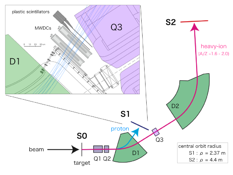
Figure 1: Schematic layout of the SHARAQ spectrometer.

In “separated flow mode”, the SHARAQ spectrometer is used as two spectrometers with different magnet configurations, “Q1-Q2-D1” and “Q1-Q2-D1-Q3-D2”. The reaction products from the target (S0) are separated and analyzed in either of these two configurations depending on their $A/Z$ values. The particles with $A/Z\sim 1$ such as protons are analyzed in the “Q1-Q2-D1” configuration and detected at the S1 focal plane, which is at the low-momentum side of the exit of the D1 magnet. On the other hand, the heavy-ion products are analyzed in the “Q1-Q2-D1-Q3-D2” configuration to increase the resolving power, and detected at the S2 final focal plane. Therefore, this new technique enables us to perform the coincidence measurements of the proton and heavy-ion pairs produced from the decays of proton-unbound states in nuclei.

In this new mode of SHARAQ, we have planned exeperiments with the parity-transfer $({}^{16}{\rm O},{}^{16}{\rm F}(0^{-},{\rm g.s.}))$ reaction. In these experiments, the outgoing ${}^{15}{\rm O}+p$ pairs produced in the decay of ${}^{16}{\rm F}$ are measured in coincidence. For the clear identification of ${}^{16}{\rm F}(0^{-})$, a high relative energy resolution of $\sim 100~{}{\rm keV}$ at $E_{\rm rel}=535~{}{\rm keV}$ is required. Furthermore, a energy resolution of ${}^{16}{\rm F}$ should be better than $\sim 2~{}{\rm MeV}$ to use the reaction as a missing-mass spectroscopy tool. These requirements can be achieved with the momentum and angular resolutions of $\delta p/p<1/300$ $(1/4500)$ and $\theta<4$ $(4)~{}{\rm mrad}$ for proton (${}^{15}{\rm O}$) for a beam energy of $250~{}{\rm MeV/u}$.

In order to achieve sufficient momentum and angular resolutions, we consider the ion-optical properties of the spectrometer in the transfer-matrix formalism. The trajectory of a particle from the target to the focal plane can be described by using the first-order terms of transfer matrix as

$$\begin{pmatrix}x_{\rm fp}\\ a_{\rm fp}\\ y_{\rm fp}\\ b_{\rm fp}\\ \delta\end{pmatrix}=\begin{pmatrix}(x|x)&(x|a)&0&0&(x|\delta)\\ (a|x)&(a|a)&0&0&(a|\delta)\\ 0&0&(y|y)&(y|b)&0\\ 0&0&(b|y)&(b|b)&0\\ 0&0&0&0&1\end{pmatrix}\begin{pmatrix}x_{\rm tgt}\\ a_{\rm tgt}\\ y_{\rm tgt}\\ b_{\rm tgt}\\ \delta\end{pmatrix},$$ (1)

where $x_{\rm fp(tgt)}$ and $a_{\rm fp(tgt)}$ are the horizontal position and angle of a particle at the focal plane (target), and $y_{\rm fp(tgt)}$ and $b_{\rm fp(tgt)}$ are the vertical position and angle, respectively. $\delta=\Delta p/p$ is a fractional momentum deviation from the central trajectory. For the spectroscopy, one needs to reconstruct the momentum ($\delta$) and the angle at the target position ($a_{\rm tgt}$, $b_{\rm tgt}$) by solving Eq. (1). In the focal plane, the $(x|a)$ term vanishes. Furthermore, if the beam spot size at the target position is small enough, the contributions from the terms of $(x|x)$, $(a|x)$ and $(y|y)$ are negligible. Then Eq. (1) can be easily solved as

$$\delta =\frac{x_{\rm fp}}{(x|\delta)},$$ (2)

$$a_{\rm tgt} =\frac{a_{\rm fp}-(a|\delta)\delta}{(a|a)},$$ (3)

$$b_{\rm tgt} =\frac{y_{\rm fp}}{(y|b)}.$$ (4)

Therefore, $\delta$, $a_{\rm tgt}$ and $b_{\rm tgt}$ can be reconstructed from $x_{\rm fp}$, $a_{\rm fp}$ and $y_{\rm fp}$, respectively.

In Eqs. (2)–(4), we assume that $x_{\rm tgt}=y_{\rm tgt}=0$ because of the small beam spot size of $\Delta x_{\rm tgt}$ and $\Delta y_{\rm tgt}$. This assumption brings the ambiguities of $\delta$, $a_{\rm tgt}$, and $b_{\rm tgt}$. The ambiguities $\Delta\delta$, $\Delta a_{\rm tgt}$, and $\Delta b_{\rm tgt}$ can be estimated as

$$\Delta\delta =\frac{(x|x)\Delta x_{\rm tgt}}{(x|\delta)},$$ (5)

$$\Delta a_{\rm tgt} =\frac{(a|x)\Delta x_{\rm tgt}}{(a|a)},$$ (6)

$$\Delta b_{\rm tgt} =\frac{(y|y)\Delta y_{\rm tgt}}{(y|b)}.$$ (7)

$\Delta x_{\rm tgt}$ and $\Delta y_{\rm tgt}$ are typically 1-2 mm. Thus, our requirements can be achieved with the conditions of

$$(x|\delta)/(x|x) >0.6~{}{\rm m},$$ (8)

$$\sqrt{\left(\frac{(a|x)}{(a|a)}\right)^{2}+\left(\frac{(y|y)}{(y|b)}\right)^{2}} <2~{}{\rm rad/m},$$ (9)

for proton, and

$$(x|\delta)/(x|x) >9.0~{}{\rm m},$$ (10)

$$\sqrt{\left(\frac{(a|x)}{(a|a)}\right)^{2}+\left(\frac{(y|y)}{(y|b)}\right)^{2}} <2~{}{\rm rad/m},$$ (11)

for ${}^{15}{\rm O}$. In order to achieve these ion-optical properties, first order ion-optical calculations using COSY INFINITY [18] were performed. In the following subsections, details of the ion-optical designs are described.

2.1 Ion-optical system from S0 to S1

In order to optimize the ion-optical properties for the particle trajectories from S0 to S1, the ion-optical calculations were performed in the Q1-Q2-D1 magnet configuration. In the calculations, the D1 magnet, which is a $32.7^{\circ}$ bending magnet with a radius of $\rho=4.4~{}{\rm m}$ in the standard operation of SHARAQ, was used as a $56.9^{\circ}$ bending magnet with a radius of $\rho=2.37~{}{\rm m}$. The results of the first order ion-optical calculations are shown in Fig. 2. In the left and right panels, the horizontal and vertical trajectories are shown for the particles with $x_{\rm S0}=\{0,\pm 1~{}{\rm mm}\}$, $y_{\rm S0}=\{0,\pm 1~{}{\rm mm}\}$, $a_{\rm S0}=\{0,\pm 25~{}{\rm mrad}\}$, $b_{\rm S0}=\{0,\pm 25~{}{\rm mm}\}$, and $\delta=\{0,\pm 10\%\}$. Here $x_{\rm S0}$ ($y_{\rm S0}$) and $a_{\rm S0}$ ($b_{\rm S0}$) are the horizontal (vertical) position and angle at the target, respectively. The field strengths of Q1 and Q2 are optimized to take a horizontal focus ($(x|a)=0$) and satisfy the condition of Eq. (9). $(y|b)$ has a large value of $-4.5$ so that a high angular resolution is achieved in the vertical direction, as can be seen in the right panel of Fig. 2.

Table 1 summarizes the ion-optical properties for the particle trajectories from S0 to S1. The ratio of the dispersion [$(x|\delta)_{\rm S1}=-1.56~{}{\rm m}$] and the horizontal magnification [$(x|x)_{\rm S1}=-0.36$] is $(x|\delta)_{\rm S1}/(x|x)_{\rm S1}=4.33~{}{\rm m}$, which satisfies the condition of Eq. (8). The resulting resolving power is $p/\delta p=4330$ for a monochromatic image size of $\Delta x_{\rm S0}=1~{}{\rm mm}$. Because of a large value of $|(a|a)_{\rm S1}|=2.75$, a high angular resolution of $\Delta a<1~{}{\rm mrad}$ can be achieved in the horizontal direction. On the other hand, in the vertical direction, the angular resolution is somewhat worse ($\Delta b=2~{}{\rm mrad}$) due to a large value of $|(y|y)_{\rm S1}|=9.00$.

In the actual trajectories from S0 to S1, the particles pass far from the central orbit of the D1 magnet, where a field homogeneity is not good. Therefore, we should consider the effects of higher order aberrations. For this purpose, the measurements using a proton beam were performed. The details of the measurements will be described in Section 3.2.

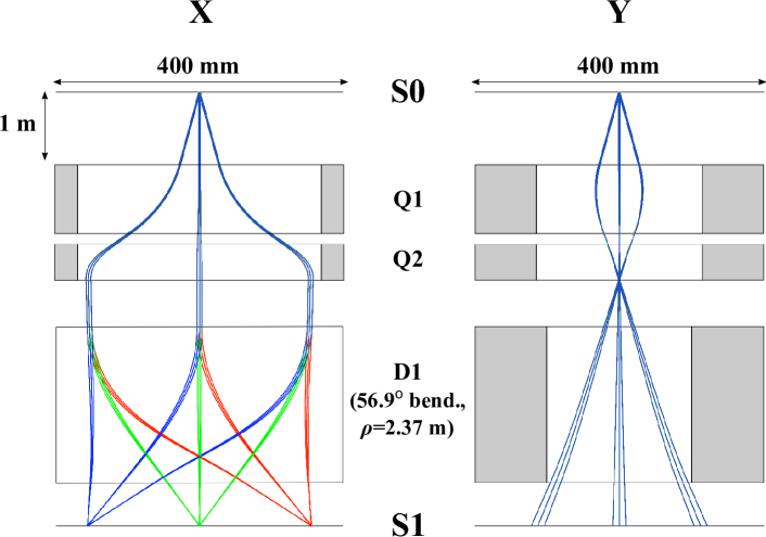
Figure 2: Results of the ion-optical calculations for the particle trajectories from S0 to S1. Left and right panels represent horizontal and vertical trajectories, respectively, for the particles with $x_{\rm S0}=\{0,\pm 1~{}{\rm mm}\}$, $y_{\rm S0}=\{0,\pm 1~{}{\rm mm}\}$, $a_{\rm S0}=\{0,\pm 25~{}{\rm mrad}\}$, $b_{\rm S0}=\{0,\pm 25~{}{\rm mrad}\}$, and $\delta=\{0,\pm 10\%\}$.

Operation mode	separated flow mode
$(x|x)_{\rm S1}$	-0.36
$(x|a)_{\rm S1}$ [m/rad]	0.00
$(x|\delta)_{\rm S1}$ [m]	-1.56
$(a|x)_{\rm S1}$ [rad/m]	-1.53
$(a|a)_{\rm S1}$	-2.75
$(a|\delta)_{\rm S1}$ [rad]	-0.75
$(y|y)_{\rm S1}$	-9.00
$(y|b)_{\rm S1}$ [m/rad]	-4.50
Resolving power (for image size of 1 mm)	4330
Horizontal angular resolution (for image size of 1 mm) [mrad]	$<1$
Vertical angular resolution (for image size of 1 mm) [mrad]	2
Momentum acceptance	$\pm 12\%$
Horizontal acceptance [mrad]	$\pm 27$
Vertical acceptance [mrad]	$\pm 25$
Solid angle [msr]	2.2

Table 1: Design parameters of the ion-optical system from S0 to S1.

2.2 Ion-optical system from S0 to S2

The results of the first order ion-optical calculations for the particle trajectories from S0 to S2 are shown in Fig. 3. Left and right panels represent the horizontal and vertical trajectories for the particles with $x_{\rm S0}=\{0,\pm 1~{}{\rm mm}\}$, $y_{\rm S0}=\{0,\pm 1~{}{\rm mm}\}$, $a_{\rm S0}=\{0,\pm 20~{}{\rm mrad}\}$, $b_{\rm S0}=\{0,\pm 50~{}{\rm mm}\}$, and $\delta=\{0,\pm 1\%\}$. It should be noted that the field strengths of Q1 and Q2 are optimized to satisfy the ion-optical design for the trajectories from S0 to S1. The remaining parameter Q3 is adjusted to take a horizontal focus [$(x|a)_{\rm S2}=0$] at the S2 focal plane. The ion-optical properties are summarized in Table 2. We can see that the designed parameters satisfy the conditions of Eqs. (10) and (11). For comparison, the design parameters for the standard mode are also shown. The new ion-optical design keeps a high resolving power of $p/\delta p=15300$ and a high angular resolution of $<1~{}{\rm mrad}$, while the horizontal angular acceptance is about 30% smaller than that for the standard mode. We also performed the ion-optical calculations in combination with the SHARAQ high-resolution beam line [10], and found that the lateral and angular dispersion-matching conditions are satisfied also for the new operation mode.

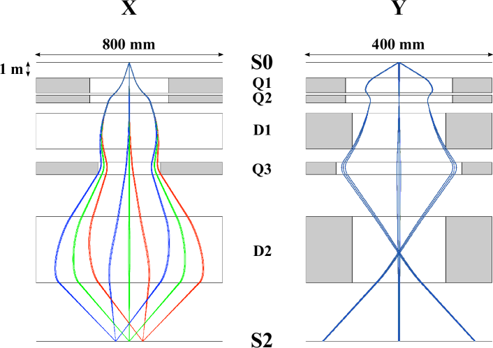
Figure 3: Results of the ion-optical calculations for the particle trajectories from S0 to S2. Left and right panels represent horizontal and vertical trajectories, respectively, for the particles with $x_{\rm S0}=\{0,\pm 1~{}{\rm mm}\}$, $y_{\rm S0}=\{0,\pm 1~{}{\rm mm}\}$, $a_{\rm S0}=\{0,\pm 20~{}{\rm mrad}\}$, $b_{\rm S0}=\{0,\pm 50~{}{\rm mm}\}$, and $\delta=\{0,\pm 1\%\}$.

Operation mode	separated flow mode	standard mode
$(x|x)_{\rm S2}$	-0.38	-0.40
$(x|a)_{\rm S2}$ [m/rad]	0.00	0.00
$(x|\delta)_{\rm S2}$ [m]	-5.81	-5.86
$(a|x)_{\rm S2}$ [rad/m]	-0.74	-0.87
$(a|a)_{\rm S2}$	-2.65	-2.50
$(a|\delta)_{\rm S2}$ [rad]	0.65	0.65
$(y|y)_{\rm S2}$	-1.11	0.00
$(y|b)_{\rm S2}$ [m/rad]	-3.26	-2.20
Resolving power (for image size of 1 mm)	15300	14700
Angular resolution (for image size of 1 mm) [mrad]	$<1$	$<1$
Momentum acceptance	$\pm 1\%$	$\pm 1\%$
Horizontal acceptance [mrad]	$\pm 20$	$\pm 30$
Vertical acceptance [mrad]	$\pm 50$	$\pm 50$
Solid angle [msr]	3.2	4.8

Table 2: Design parameters of the ion-optical system from S0 to S2. The design parameters for the standard mode of SHARAQ are also shown for comparison.

2.3 Dispersion mismatch between beam line and ion-optical system from S0 to S1

When the disperion-matched transport is used with the separated flow mode, the lateral and angular dispersion-matching conditions are satisfied between the beam line and the ion-optical system from S0 to S2. These conditions are exprressed as

$$(x|x)_{\rm S2}(x|\delta)_{\rm bl}+(x|a)_{\rm S2}(a|\delta)_{\rm bl}+(x|\delta)_{\rm S2}=0,$$ (12)

$$(a|x)_{\rm S2}(x|\delta)_{\rm bl}+(a|a)_{\rm S2}(a|\delta)_{\rm bl}+(a|\delta)_{\rm S2}=0,$$ (13)

where $(x|\delta)_{\rm bl}$ and $(a|\delta)_{\rm bl}$ are the matrix elements in the beam line. Then $(x|\delta)_{\rm bl}=-15.3~{}{\rm m}$ and $(a|\delta)_{\rm bl}=4.5~{}{\rm rad}$ are obtained from Eqs. (12) and (13). Apparently, the dispersion-matching conditions can not be satisfied at S1 with the same beam-line setting as:

$$(x|x)_{\rm S1}(x|\delta)_{\rm bl}+(x|a)_{\rm S1}(a|\delta)_{\rm bl}+(x|\delta)_{\rm S1}=3.9~{}{\rm m},$$ (14)

$$(a|x)_{\rm S1}(x|\delta)_{\rm bl}+(a|a)_{\rm S1}(a|\delta)_{\rm bl}+(a|\delta)_{\rm S1}=10.2~{}{\rm rad}.$$ (15)

The non-zero values of Eqs. (14) and (15) bring uncertainties in $\delta$ and $a_{\rm S0}$ of protons, respectively, according to the momentum spread of the beam $\Delta p/p$. Since $\Delta p/p$ is typically $0.1\%$, the ambiguities are estimated to be $\Delta x_{\rm S1}=3.9~{}{\rm mm}$ and $\Delta a_{\rm S1}=10.2~{}{\rm mrad}$ at S1, which correspond to the ambiguities of $\Delta\delta=1/400$ and $\Delta a_{\rm S0}=3.7~{}{\rm mrad}$ in the reconstruction of Eqs. (2) and (3). These ambiguities are comparable to our required resolutions. Therefore we conclude that the dispersion mismatch between the beam line and the ion-optical system from S0 to S1 has no significant effect on our requirements.

3 Experiments

3.1 Experimental setup at S1

For the measurements with the separated flow mode of SHARAQ, we have developed a tracking detector system at the S1 focal plane. This system consists of two multi-wire drift chambers (MWDCs) and two plastic scintillators, as shown in Fig. 1. Table 3 shows the specifications of the MWDCs. This MWDC is basically an atmospheric operational version of low-pressure multi-wire drift chambers (LP-MWDCs) in Ref. [19]. Each MWDC has an X-X’-Y-Y’ configuration and an effective area of $480~{}{\rm mm}^{W}\times 240~{}{\rm mm}^{H}$. The position resolution and the detection efficiency are typically $300~{}\mu{\rm m}$ (FWHM) and $>95\%$, respectively, for $250~{}{\rm MeV}$ protons. The MWDCs are installed with a separation of 200 mm crossing the S1 focal plane. Thus the position and angular resolutions in the S1 focal plane are typically $200~{}\mu{\rm m}$ and $2~{}{\rm mrad}$, respectively. The readout electronics and data acquisition (DAQ) system are the same as those described in Ref. [19]. The vaccum and the air are separated at the exit of the D1 magnet by a kapton film with a thickness of $125~{}\mu{\rm m}$, which causes an angular straggling of about 1 mrad for $250~{}{\rm MeV}$ protons.

Configuration	X - X’ - Y - Y’
Effective area	$480~{}{\rm mm}^{W}\times 240~{}{\rm mm}^{H}$
Cell size	$12~{}{\rm mm}^{W}\times 10~{}{\rm mm}^{t}$
Numbers of channels	120
Anode wire	Au-W, 20 $\mu{\rm m}^{\phi}$
Potential wire	Cu-W, 80 $\mu{\rm m}^{\phi}$
Cathode plane	Al-Mylar, 2 $\mu{\rm m}^{t}$
Counter gas	P10 : Ar - ${\rm CH}_{4}$ (90 - 10), 1 atm
Gas window	Al-Mylar, 25 $\mu{\rm m}^{t}$
Potential Voltage	$-1.65~{}{\rm kV}$
Cathode Voltage	$-1.50~{}{\rm kV}$

Table 3: Specifications of the MWDCs at S1. The X’ (Y’) plane is offset by half cell from the X (Y) plane.

3.2 Ion-optics study with proton beam

In order to study the ion-optical properties between S0 and S1, we measured the trajectories from S0 to S1 by using a proton beam. A secondary proton beam at 246 MeV was produced by the BigRIPS [20] using a primary ${}^{16}{\rm O}$ beam at $247~{}{\rm MeV/{\rm u}}$ with a typical intensity of 10 particle nA in a 4-mm thick Be target. The secondary beam was transported to the SHARAQ spectrometer by using the high-resolution beam line with the high-resolution achromatic transport mode [9]. A typical intensity of the secondary beam was $1~{}{\rm kcps}$ at S0. In order to track the beam trajectories, LP-MWDCs [19] and MWDCs described in Sec. 3.1 were used at S0 and S1, respectively. The beam profile measured at S0 was $\sigma_{x}=6~{}{\rm mm}$ and $\sigma_{a}=11~{}{\rm mrad}$ in the horizontal direction, and $\sigma_{y}=8~{}{\rm mm}$ and $\sigma_{b}=5~{}{\rm mrad}$ in the vertical direction. The momentum spread of the beam was about $\pm 0.1\%$.

We obtained the transfer matrix elements from S0 to S1 by using the correlations of the measured beam trajectories at S0 and S1. For example, a correlation between the horizontal angle at S1 ($a_{\rm S1}$) and the horizontal angle at S0 ($a_{\rm S0}$) provides us with a measure of the $(a|a)$ element. The left panel in Fig. 4 shows the correlation between $a_{\rm S1}$ and $a_{\rm S0}$. The gradient of the correlation corresponds to the $(a|a)$ element. The second order gradient is also seen, which corresponds to the $(a|aa)$ element. Thus, $(a|a)=-3.03\pm 0.01$ and $(a|aa)=-24.0\pm 0.8~{}{\rm rad}^{-1}$ are obtained in this case. We also determined the $\delta$ dependent terms of the matrix elements by scaling the magnet field of the spectrometer because scaling of the magnet field changes $\delta$ effectively. The right panel in Fig. 4 shows the $a_{\rm S1}$-$a_{\rm S0}$ correlations for various magnetic field settings. Five loci in the figure represent the events for scaling factors of 0.930, 0.965, 1.000, 1.035, and 1.070, which correspond to $\delta=+7.0\%,+3.5\%,0.0\%,-3.5\%,$ and $-7.0\%$, respectively. The difference of the gradients between the five loci corresponds to the matrix elements such as $(a|a\delta)$ and $(a|aa\delta)$. The matrix elements such as $(a|\delta)$ and $(a|\delta\delta)$ are also obtained from the shift of the $a_{\rm S1}$ positions at $a_{\rm S0}=0~{}{\rm mrad}$.

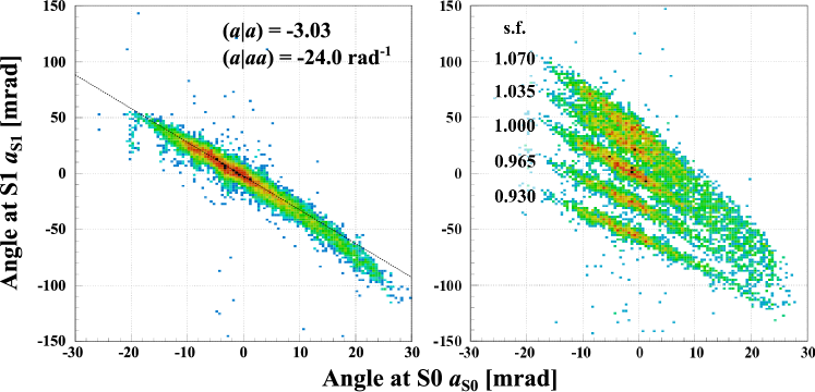
Figure 4: Correlation between the horizontal angle at the focal plane S1 and the horizontal angle at the focal plane S0 for a proton beam.

Table 4 summarize the measured matrix elements from S0 to S1. For the first order terms, the measured matrix elements are in good agreement with the design values in Table 1. We also found that the effects of the higher order terms were enough large to change the trajectories, and that these effects should be correctly taken into account.

We reconstructed the beam momentum and angles at S0 from the beam trajectory at S1 using an inverse matrix determined by the measured matrix elements. In the reconstruction, the events in a region of $|x_{\rm S0}|<0.5~{}{\rm mm}$ and $|y_{\rm S0}|<0.5~{}{\rm mm}$ were selected, and $x_{\rm S0}$ and $y_{\rm S0}$ values were set to $x_{\rm S0}=y_{\rm S0}=0$. Figure 5 shows the $\delta$ values reconstructed from the beam trajectory at S1. Five peaks correspond to the events for different magnet field settings. The $\delta$ value for each peak is well reproduced according to the corresponding scaling factor. The width for each peak varies between $0.28\%$ and $0.33\%$ FWHM depending on $\delta$, which is mainly due to the momentum spread of the beam of about $\pm 0.1\%$.

We also compared the $a_{\rm S0}$ and $b_{\rm S0}$ values reconstructed from the beam trajectory at S1 with those measured by MWDCs at S0 in Fig. 6. Top panels show the correlations between the reconstructed and measured values, and bottom panels take the differences between these values. We can see that both the $a_{\rm S0}$ and $b_{\rm S0}$ values are properly reconstructed. The widths of the difference distributions are 3.8 and 7.2 mrad FWHM for $a_{\rm S0}$ and $b_{\rm S0}$, respectively, main parts of which arise from the position and angular resolutions at S0 (3 mm and 2 mrad FWHM).

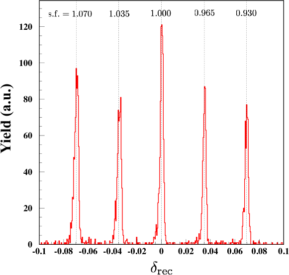
Figure 5: The $\delta$ values reconstructed from the beam trajectory at S1.

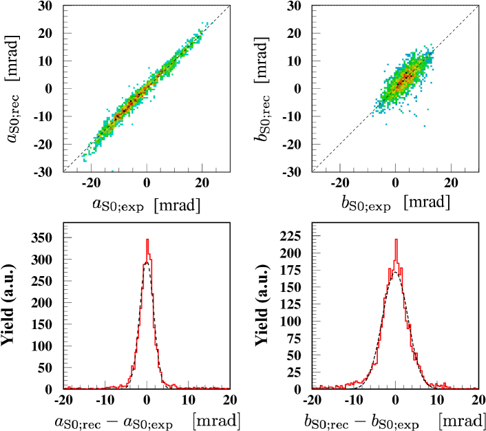
Figure 6: The $a_{\rm S0}$ and $b_{\rm S0}$ values reconstructed from the beam trajectory at S1. Top panels show the correlations between the reconstructed and measured values, and bottom panels take the differences between these values.

$x$		$a$		$y$
$(x|x)_{\rm S1}$	$-0.34\pm 0.01$	$(a|x)_{\rm S1}$	$-1.43\pm 0.01$	$(y|y)_{\rm S1}$	$-9.55\pm 0.02$
$(x|a)_{\rm S1}$	$0.01\pm 0.01$	$(a|a)_{\rm S1}$	$-3.03\pm 0.01$	$(y|b)_{\rm S1}$	$-4.70\pm 0.05$
$(x|\delta)_{\rm S1}$	$-1.5703\pm 0.0002$	$(a|\delta)_{\rm S1}$	$-0.70\pm 0.05$
$(x|aa)_{\rm S1}$	$0.80\pm 0.74$	$(a|aa)_{\rm S1}$	$-24.0\pm 0.8$	$(y|ab)_{\rm S1}$	$-36\pm 3$
$(x|a\delta)_{\rm S1}$	$0.40\pm 0.14$	$(a|a\delta)_{\rm S1}$	$11.5\pm 0.2$	$(y|y\delta)_{\rm S1}$	$34.0\pm 0.4$
$(x|\delta\delta)_{\rm S1}$	$-7.319\pm 0.001$	$(a|\delta\delta)_{\rm S1}$	$1.5\pm 0.2$	$(y|b\delta)_{\rm S1}$	$23.5\pm 0.9$
$(x|aaa)_{\rm S1}$	$-820\pm 31$	$(a|aa\delta)_{\rm S1}$	$80\pm 16$	$(y|ab\delta)_{\rm S1}$	$231\pm 73$
$(x|a\delta\delta)_{\rm S1}$	$-57\pm 1$	$(a|a\delta\delta)_{\rm S1}$	$-12\pm 4$	$(y|b\delta\delta)_{\rm S1}$	$-74\pm 19$
$(x|\delta\delta\delta)_{\rm S1}$	$-29.23\pm 0.05$	$(a|\delta\delta\delta)_{\rm S1}$	$8\pm 6$

Table 4: Measured transfer matrix elements from S0 to S1. Units for lengths and angles are in meter and radian, respectively.

3.3 Measurement of $({}^{16}{\rm O},{}^{16}{\rm F})$ reaction

The performance of the separated flow mode was studied by using the $({}^{16}{\rm O},{}^{16}{\rm F})$ reaction. A primary ${}^{16}{\rm O}$ beam at $247~{}{\rm MeV/u}$ and $10^{7}~{}{\rm pps}$ was transported to the S0 target position. The beam line to the spectrometer was set up for the dispersion matched transport. A plastic scintillator with a thickness of $1~{}{\rm mm}$ was used as a reaction target. The outgoing ${}^{15}{\rm O}+p$ produced by the decay of ${}^{16}{\rm F}$ were measured in coincidence. The particles were momentum analyzed by using the SHARAQ spectrometer. The ${}^{15}{\rm O}$ particles were detected with two LP-MWDCs at the S2 focal plane, while the protons were detected with two MWDCs at the S1 focal plane.

Figure 7 represents the correlations between the position (angle) at S2 and the position at F6 for the ${}^{16}{\rm O}$ beam. Here F6 is a dispersive focal plane of the beam line, and the position was measured by a parallel plate avalanche counter (PPAC). The position at F6 corresponds to the beam momentum. Upright correltions found in the figures indicate that the position and angle at S2 are independent of the beam momentum, which demonstrates that the lateral and angular dispersion-matching conditions are satisfied also for the separated flow mode.

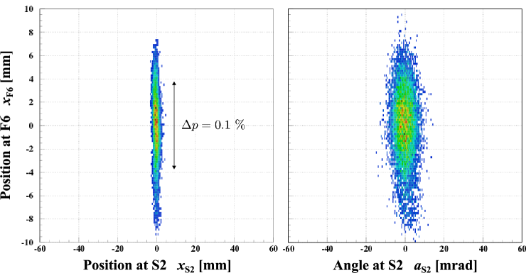
Figure 7: Correlation between $x_{\rm F6}$ and the position (left) and angle (right) at S2 for a ${}^{16}{\rm O}$ beam at 247 MeV/u. Upright correlations observed in the figures indicate that the lateral and angular dispersion-matching conditions are fulfilled.

Figure 8 shows a two-dimentional plot of the proton momentum and the opening angle between the ${}^{15}{\rm O}$ particle and the proton. The dashed curves indicate the relative energy $E_{\rm rel}$ between the ${}^{15}{\rm O}$ particle and the proton in $0.2~{}{\rm MeV}$ step. As can be seen, three states of ${}^{16}{\rm F}$ with $J^{\pi}~{}=~{}0^{-},1^{-}$, and $2^{-}$ at $E_{\rm rel}~{}=~{}0.535,0.728$, and 0.959 MeV are clearly separated. The obtained $E_{\rm rel}$ resolution is 100 keV FWHM at $E_{\rm rel}~{}=~{}0.535~{}{\rm MeV}$, which satisfies our requirement.

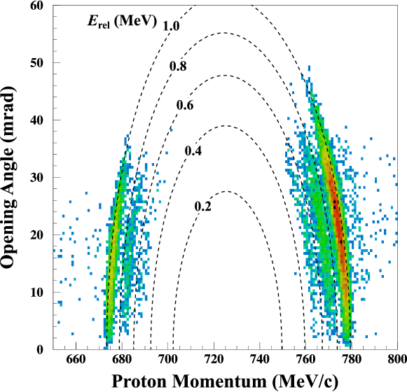
Figure 8: Two-dimentional plot of the proton momentum and the opening angle between the ${}^{15}{\rm O}$ particle and the proton. The dashed curves indicate the relative energy between the ${}^{15}{\rm O}$ particle and the proton in $0.2~{}{\rm MeV}$ step.

We also estimated the detection efficiency for the ${}^{15}{\rm O}+p$ coincidence events from the Monte Carlo simulation, where the acceptance and the finite resolution in angles and momenta are taken into account. The result is shown in Fig. 9, as a funciton of $E_{\rm rel}$. The obtained efficiency is 0.189 at $E_{\rm rel}=0.535~{}{\rm MeV}$, which is mainly due to the angular acceptance for the proton.

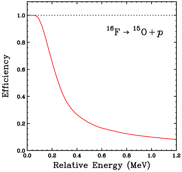
Figure 9: Detection efficiency for the ${}^{15}{\rm O}+p$ coincidence events calculated by Monte Carlo simulations, as a funciton of relative energy.

Figure 10 shows the kinetic-energy distribution of ${}^{16}{\rm F}$ for the $({}^{16}{\rm O},{}^{16}{\rm F})$ reaction at a reaction angle of $\theta_{\rm reac}<2~{}{\rm mrad}$. A prominent peak at $E({}^{16}{\rm F})\sim 3940~{}{\rm MeV}$ corresponds to the $({}^{16}{\rm O},{}^{16}{\rm F})$ reaction on hydrogens in the plastic scintillator. The width is about 2.8 MeV FWHM. The intrinsic energy resolution is about 2.1 MeV FWHM by considering the energy straggling of the particles in the target ($\sim 1.8~{}{\rm MeV}$). Thus our requirement is satisfied also for the ${}^{16}{\rm F}$ energy resolution.

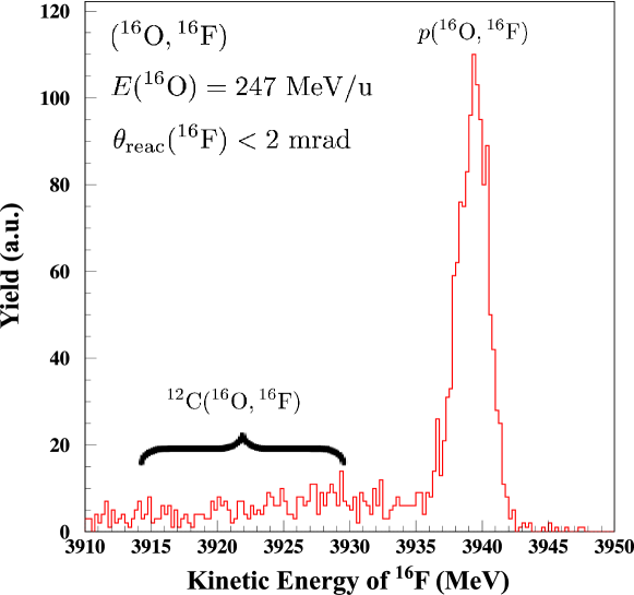
Figure 10: Kinetic-energy distribution of ${}^{16}{\rm F}$ for the $({}^{16}{\rm O},{}^{16}{\rm F})$ reaction at $\theta_{\rm reac}<2~{}{\rm mrad}$.

4 Summary

New operation mode, “separated flow mode”, has been developed for in-flight proton decay experiments with the SHARAQ spectrometer. The concept of the separated flow mode is the use of the SHARAQ spectrometer as two spectrometers with different magnet configurations, which allows the coincidence measurements of the proton and heavy-ion pairs produced from the decays of proton-unbound states in nuclei.

The ion-optical properties of the new mode were studied by using a proton beam at 246 MeV. The transfer matrix elements were experimentally determined including the higher order terms, and the momentum vector was properly reconstructed from the parameters measured in the focal plane of SHARAQ.

The separated flow mode was successfully introduced in the experiment with the $({}^{16}{\rm O},{}^{16}{\rm F})$ reaction at a beam energy of 247 MeV/u. The outgoing ${}^{15}{\rm O}+p$ produced by the decay of ${}^{16}{\rm F}$ were measured in coincidence with SHARAQ. High energy resolutions of 100 keV (FWHM) and $\sim 2~{}{\rm MeV}$ were achieved for the relative energy of 535 keV, and the ${}^{16}{\rm F}$ energy of 3940 MeV, respectively. Such an accurate missing-mass measurement combined with an invariant-mass method gives a unique opportunity to explore little-studied excitation modes in nuclei by using new types of reaction probes with particle decay channels.

References

- [1] N. Iwasa et al., Phys. Rev. Lett. 83 (1999) 2910–2913. doi:10.1103/PhysRevLett.83.2910.
- [2] P. Senger et al., Nuclear Instruments and Methods in Physics Research Section A: Accelerators, Spectrometers, Detectors and Associated Equipment 327 (1993) 393 – 411. doi:http://dx.doi.org/10.1016/0168-9002(93)90706-N.
- [3] T. Nakamura et al., Phys. Rev. Lett. 96 (2006) 252502. doi:10.1103/PhysRevLett.96.252502.
- [4] Y. Kondo et al., Physics Letters B 690 (2010) 245 – 249. doi:http://dx.doi.org/10.1016/j.physletb.2010.05.031.
- [5] Y. Shimizu et al., Journal of Physics: Conference Series 312 (2011) 052022.
- [6] T. Kobayashi et al., Nuclear Instruments and Methods in Physics Research Section B: Beam Interactions with Materials and Atoms 317, Part B (2013) 294 – 304. doi:http://dx.doi.org/10.1016/j.nimb.2013.05.089.
- [7] T. Uesaka et al., Nuclear Instruments and Methods in Physics Research Section B: Beam Interacions with Materials and Atoms 266 (2008) 4218 – 4222. doi:http://dx.doi.org/10.1016/j.nimb.2008.05.095.
- [8] T. Uesaka et al., Prog. Theor. Exp. Phys. 2012 (2012) 03C007. doi:10.1093/ptep/pts042.
- [9] S. Michimasa et al., Nuclear Instruments and Methods in Physics Research Section B: Beam Interactions with Materials and Atoms 317, Part B (2013) 305 – 310. doi:http://dx.doi.org/10.1016/j.nimb.2013.08.060.
- [10] T. Kawabata et al., Nuclear Instruments and Methods in Physics Research Section B: Beam Interactions with Materials and Atoms 266 (2008) 4201 – 4204. doi:http://dx.doi.org/10.1016/j.nimb.2008.05.026.
- [11] T. Uesaka et al., Progress of Theoretical Physics Supplement 196 (2012) 150–157. doi:10.1143/PTPS.196.150.
- [12] T. Uesaka, Journal of Physics: Conference Series 445 (2013) 012018.
- [13] K. Miki et al., Phys. Rev. Lett. 108 (2012) 262503. doi:10.1103/PhysRevLett.108.262503.
- [14] S. Noji, Ph.D. thesis, The University of Tokyo (2012).
- [15] Y. Sasamoto, Ph.D. thesis, The University of Tokyo (2012).
- [16] K. Kisamori, Ph.D. thesis, The University of Tokyo (2015).
- [17] M. Dozono, RIKEN Accel. Prog. Rep. 45 (2012) 10.
- [18] K. Makino, M. Berz, Nuclear Instruments and Methods in Physics Research Section A: Accelerators, Spectrometers, Detectors and Associated Equipment 558 (2006) 346 – 350. doi:http://dx.doi.org/10.1016/j.nima.2005.11.109.
- [19] H. Miya et al., Nuclear Instruments and Methods in Physics Research Section B: Beam Interactions with Materials and Atoms 317, Part B (2013) 701 – 704. doi:http://dx.doi.org/10.1016/j.nimb.2013.08.018.
- [20] T. Kubo, Nuclear Instruments and Methods in Physics Research Section B: Beam Interactions with Materials and Atoms 204 (2003) 97 – 113. doi:http://dx.doi.org/10.1016/S0168-583X(02)01896-7.