Collision strengths and transition probabilities for Co iii forbidden lines

Abstract

In this paper we compute the collision strengths and their thermally-averaged Maxwellian values for electron transitions between the fifteen lowest levels of doubly-ionised cobalt, Co²⁺, which give rise to forbidden emission lines in the visible and infrared region of spectrum. The calculations also include transition probabilities and predicted relative line emissivities. The data are particularly useful for analysing the thermodynamic conditions of supernova ejecta.

1 Introduction

Cobalt is an iron-group element but is the least abundant of this group with a solar abundance of about 300 times less than Fe. However, in supernova (SN) ejecta it is much more abundant. For example, in SN 1987A the ratio of Co to Fe, 255 days after outburst, is approximately 0.2 by number (Varani et al, 1990). The spectral lines of Co are therefore valuable investigative tools in analysing the chemical and thermodynamic conditions of supernovae where these emissions are mostly found. These lines are also useful in investigating the evolutionary history and chemical development by nucleosynthesis and decay processes within the SN explosions (Colgate & McKee, 1969; Axelrod, 1980; Kuchner et al, 1994; Bowers et al, 1997; Liu et al, 1997; Churazov et al, 2014; Childress et al, 2015). The lines of Cobalt have also been observed in the spectral emissions of astronomical objects with more normal Co abundances such as planetary nebulae (Baluteau et al, 1995; Zhang et al, 2005; Pottasch & Surendiranath, 2005; Wang & Liu, 2007; Fang & Liu, 2011).

Little computational and experimental work has been done previously to generate essential atomic data for Co iii and none of the previous work deals with excitation of Co²⁺ levels by electron impact. Hansen et al (1984) calculated magnetic dipole and electric quadrupole transition probabilities in the 3d⁷ ground configuration of Co iii using parametric fitting to the observed energy levels and Hartree-Fock values for the electric quadrupole moments. In their investigation of the forbidden transition probabilities relevant to the analysis of infrared lines from SN 1987A, Nussbaumer & Storey (1988) provided a few transition probabilities for low levels of Co iii assuming $LS$-coupling. Tankosić et al (2003) calculated Stark broadening data for a number of Co iii spectral lines as a function of temperature by using a semi-empirical approach. Experimental investigations have also been conducted by Sugar & Corliss (1981, 1985) where atomic data related to Co iii transitions, mainly energy levels of Co²⁺, have been collected. Very recently, Fivet et al (2016) calculated radiative probabilities of Co iii forbidden transitions between low-lying levels of doubly ionised cobalt as part of a larger investigation of the radiative rates in doubly ionised iron-peak elements.

We have recently reported a calculation of atomic parameters for energetically low-lying levels of Co⁺ (Storey et al, 2016). In this paper we present a similar calculation of atomic parameters related to forbidden transitions in Co²⁺, which includes lines ranging from the visible to the three mid-infrared lines which arise from transitions within the ground term at 11.88, 16.39 and 24.06 $\mu$m. The paper primarily addresses a shortage in collisional atomic data which forced some researchers (Dessart et al, 2014; Childress et al, 2015) to adopt collision strengths generated for Ni iv (Sunderland et al, 2002) as a substitute for corresponding data of Co iii justifying this by the fact that the two ions possess similar electronic and term structures. Our principal result is collision strengths and their thermally-averaged Maxwellian values for electron excitation and de-excitation between the fifteen lowest levels of Co²⁺. The study also includes the most important radiative transition probabilities for the same levels. The main tools used in generating these data are the R-matrix atomic scattering code (Berrington et al, 1974, 1987; Hummer et al, 1993; Berrington et al, 1995) and the general purpose Autostructure code (Eissner et al, 1974; Nussbaumer & Storey, 1978; Badnell, 2011). The scattering calculations were performed using a 10-configuration atomic target within a Breit-Pauli intermediate coupling approximation, as will be detailed in Section 2.

The paper is structured as follow. In Section 2 the Co²⁺ model is presented and the resulting transition probabilities are given, whereas in Section 3 the Breit-Pauli R-matrix Co${}^{2+}+e$ scattering calculation is described. Results and general analysis related to the diagnostic potentials of some transitions appear in Section 4, and section 5 concludes the paper.

2 Co²⁺ Atomic Structure

2.1 The scattering target

A schematic diagram of the term structure of Co iii up to 1.5 Rydberg is shown in Figure 1. The extent of our target is shown by the heavy solid line in that figure and includes 36 terms and 109 levels. The lowest 21 terms of this ion are of even parity from the configurations 3d⁷ and 3d⁶4s. Transitions from higher terms give rise to lines that should be weaker at the typical temperatures of supernova ejecta and hence they will be ignored. The odd-parity terms of the 3d⁶4p configuration are expected to give rise to resonances that affect the collision strengths for excitation of the low-lying even-parity levels and hence they are included in the target for the scattering calculations.

Figure 1: Schematic term energy diagram of Co iii. The heavy solid line shows the extent of the close-coupled target states.

A set of ten electron configurations, listed in Table 1, were used to expand the target states. The target wavefunctions were generated with the Autostructure program, (Eissner et al, 1974; Nussbaumer & Storey, 1978; Badnell, 2011) using radial functions computed within scaled Thomas-Fermi-Dirac statistical model potentials. The scaling parameters were determined by minimising the sum of the energies of all the target terms, computed in $LS$-coupling, i.e. by neglecting all relativistic effects. The resulting scaling parameters, $\lambda_{nl}$, are given in Table 2.

Table 1: The ten target configuration basis where the core electronic structure ([Ar]) is suppressed. The bar indicates a correlation orbital.

3d7

3d6 4s, 4p, $\overline{4}$d

3d5 4s2, 4p2, $\overline{4}$d2, 4s4p, 4s$\overline{4}$d, 4p$\overline{4}$d

Table 2: Potential scaling parameters. The bar over the principal quantum number signifies a correlation orbital.

1s	1.42912
2s	1.13799	2p	1.08143
3s	1.06915	3p	1.05203	3d	1.04962
4s	1.03440	4p	1.02977	$\overline{4}$d	1.51187

In Table 3 a comparison is made between the term energies calculated using our scattering target with experimental values for the 36 terms of the target. The term energies are computed with the inclusion of one-body relativistic effects, the Darwin and mass terms, and the spin-orbit interaction. This is the type of approximation that we applied for the scattering calculations in the R-matrix code. In Table 4 the calculated energies of the 15 lowest levels are compared with the corresponding experimental values. The table also shows the values obtained by including the two-body fine structure interactions as described by Eissner et al (1974). The calculated fine-structure splittings of these levels are improved by this inclusion. For the total fine-structure splitting of the six terms, the average absolute difference from experiment drops from 7.3% to 4.6%.

Table 3: Energies of the 36 target terms in cm^-1, ordered according to the experimental energy. The calculated values include only the spin-orbit contribution to the fine-structure energies. Core electronic structure ([Ar]) is suppressed from all configurations.

		Term Energy
Config.	Term	Exp.†	Calc.
3d7	a4F	0	0
	a4P	14561	17891
	a2G	16510	19120
	a2P	19618	25103
	a2H	22227	25205
	a2D	22712	27507
	a2F	36372	43416
3d64s	a6D	46230	48501
	a4D	55448	58817
	b4P	70965	79599
	a4H	71096	76483
	b4F	72717	80163
	a4G	76219	83370
	b2P	76521	85780
	b2H	76690	82428
	b2F	78323	86408
	b2G	81793	89400
	b4D	83031	92162
	a2I	84676	91484
	c2G	85485	93867
	b2D	90897	98436
3d64p	z6Do	97807	97268
3d64s	2S		100359
3d64p	z6Fo	102620	102460
3d64s	2D		103690
3d64p	z6Po	104861	104906
	z4Do	106074	106802
	z4Fo	106676	107272
	z4Po	109902	111225
3d64s	2F		111250
	4F		119049
	4P		119600
	2F		125226
	2P		125937
3d64p	z4So	122305	129103
	z4Go	124219	127494
†Experimental energies are from NIST (www.nist.gov).

Table 4: Energies in cm^-1 of the 15 lowest levels of Co²⁺, ordered according to the experimental energy, where the configuration of all levels is [Ar] 3d⁷.

Index	Level	Exp.1	Calc.2	Calc.3
1	$a^{4}$F9/2	0.	0.	0.
2	$a^{4}$F7/2	841	810	824
3	$a^{4}$F5/2	1451	1408	1428
4	$a^{4}$F3/2	1867	1819	1842
5	$a^{4}$P5/2	15202	18481	18502
6	$a^{4}$P3/2	15428	18770	18785
7	$a^{4}$P1/2	15811	19125	19118
8	$a^{2}$G9/2	16978	19565	19581
9	$a^{2}$G7/2	17766	20348	20357
10	$a^{2}$P3/2	20195	25601	25633
11	$a^{2}$P1/2	20919	26486	26474
12	$a^{2}$H11/2	22720	25690	25687
13	$a^{2}$D5/2	23059	27795	27804
14	$a^{2}$H9/2	23434	26367	26379
15	$a^{2}$D3/2	24237	29058	29033
1 Sugar & Corliss 1985.
2 Calculated with only spin-orbit interaction.
3 As 2 plus two-body fine-structure interactions
for the first 4 configurations of Table 1.

A widely-accepted measure for the quality of the scattering calculations is the degree of agreement between weighted oscillator strengths, $gf$, calculated in the velocity and length formulations, where good agreement is regarded as necessary but not sufficient condition for the quality of the target wavefunctions. Table 5 provides this comparison where it shows an average difference in the absolute values of $gf$ of about 5.8% between the two formulations, which in our view is acceptable for an open d-shell atomic system.

Table 5: Weighted $LS$ oscillator strengths, $gf$, in the length and velocity formulations from the two energetically lowest terms of the 3d⁷ and 3d⁶4s configurations.

	Transition					$gf_{{}_{L}}$	$gf_{{}_{V}}$
	3d7	4F	–	3d64p	4Do	2.34	2.48
			–		4Fo	1.16	1.21
			–		3Go	2.38	2.30
	3d64s	6D	–	3d64p	6Do	9.45	9.75
			–		6Fo	13.7	13.5
			–		6Po	5.77	4.83

2.2 Transition probabilities

The forbidden transition probabilities between the even parity low-lying terms are calculated using the afore-described target wavefunctions, with empirical adjustments to the computed energies to ensure more reliable calculation of the fine-structure interactions and accurate energy factors connecting the ab initio calculated line strengths to the transition probabilities. The results for the lowest 15 levels are given in Table 10 where the values represent the sum of the electric quadrupole and magnetic dipole contributions for each transition. This table includes only those probabilities from a given upper level which exceed 1% of the total probability from that level.

The infrared lines of principal interest here arise from transitions between the levels of the ground ⁴F term and are predominantly of magnetic dipole type. There is therefore a stepwise decay through the levels and only three relevant transition probabilities, for $a^{4}$F_3/2 - $a^{4}$F_5/2, $a^{4}$F_5/2 - $a^{4}$F_7/2 and $a^{4}$F_7/2 - $a^{4}$F_9/2. We are aware of only two previous calculations of transition probabilities for Co iii, one by Hansen et al (1984) and one by Nussbaumer & Storey (1988), as well as one contemporary calculation by Fivet et al (2016). Nussbaumer & Storey (1988) only give values for these three probabilities and these differ by less than 1% from our values. Hansen et al (1984) give more extensive results which we compare with the present values in Table 10. We find excellent agreement with Hansen et al (1984) for the magnetic dipole transitions between the levels of individual terms with differences of a few percent or less. There are larger differences for the electric quadrupole transition probabilities between terms. For example the probabilities for the principal transitions between the $a^{4}$F and $a^{4}$P terms, the 5-1, 5-2 and 5-3 probabilities, are all larger, by on average 13%, in our calculation than in Hansen et al (1984). The fact that all three transitions differ by approximately the same factor suggests that the cause of the difference lies in the radial quadrupole integrals used in the two calculations. There is configuration interaction between the terms of the 3d⁷ electron configuration and the 3d${}^{6}\overline{4}$d configuration in our calculation and not in the single configuration calculation of Hansen et al (1984). With this interaction included, the quadrupole line strength involves both the 3d radial quadrupole integral and the $\overline{4}$d integral which is significantly larger than for the 3d.

Fivet et al (2016) have made calculations of forbidden transition probabilities for the twice ionised iron-peak elements from Sc to Ni, including Co, and we compare with their results in Table 10. Their calculations were made with two different methods which we label as FQB1 and FQB2. The FQB2 values were computed with Autostructure as in the present work. Apart from the magnetic dipole transitions between the levels of the ground term, which agree to all tabulated figures, the FQB2 results for the electric quadrupole transitions between levels of different terms are systematically larger than the present work by 15-20% with half of them differing by the same fixed amount of 19%. As discussed above in the comparison with the work of Hansen et al (1984), the systematic nature of the difference suggests that it is due to a different value for the 3d radial quadrupole integral rather than details of the wave function expansions of individual terms. The configuration expansions in the present work and in that of Fivet et al (2016) are very similar but differ in one key aspect. We use a somewhat contracted $\overline{4}$d orbital to allow for the differences in the 3d orbital between the 3d⁷ and 3d⁶4s configurations, while Fivet et al (2016) employ a spectroscopic 4d orbital but a contracted 5s orbital which provides flexibility to the spectroscopic 4s. These two different expansions give broadly similar energy levels and fine-structure but result in differences in the quadrupole radial integrals. It is not clear that either approach is necessarily superior, so the approximately 15-20% differences are probably a realistic measure of the uncertainty in the results for the electric quadrupole line strengths. We note that the results for the electric quadrupole transition probabilities from the FQB1 calculation of Fivet et al (2016) agree better with their FQB2 for some transitions and better with the current work for others.

3 Scattering Calculations

In this work we used the Breit-Pauli R-matrix method, which is detailed in Hummer et al (1993); Berrington et al (1995) and the references therein, to perform the scattering calculations. The calculations were made using the R-matrix codes where the serial version of the codes were used in some stages and the parallel version in others. An R-matrix boundary radius of 11.3 au defining the inner region was applied so that the most extended orbital (4p) of our target is covered. Each one of the partial waves of the scattered electron was expanded over 12 basis functions within the R-matrix boundary, and the expansion extends to a maximum of $J=9$.

Collision strengths were computed over two non-overlapping energy meshes: a fine mesh consisting of 20000 evenly-divided intervals which goes from zero up to the highest target threshold (about 1.2 Rydberg), and a coarse mesh consisting of 2000 evenly-divided intervals which reach 1 Rydberg above the highest target threshold. The purpose of the first mesh is to cover the main resonance region while the second mesh is intended to cover the region where all scattering channels are open, up to an incident electron energy of about 2.2 Rydberg. Our results demonstrate that these meshes have achieved these purposes. In Figure 2 we illustrate our results with the computed collision strengths between the lowest four levels of the ground 3d^7 4F term as a function of final electron energy up to 1 Rydberg above threshold. Dense and complex resonance structure can be seen in these plots due to the multiple close lying thresholds. We also show the collision strength averaged over 0.02 Rydberg intervals.

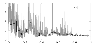
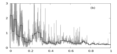
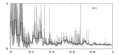
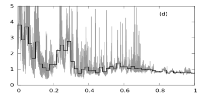
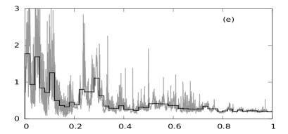
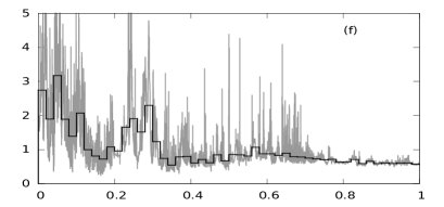
Figure 2: Collision strength (vertical axis) versus final electron energy in Rydberg (horizontal axis) for the (a) 1-2, (b) 1-3, (c) 1-4, (d) 2-3, (e) 2-4 and (f) 3-4 transitions, where the grey smooth line represents the continuous function while the black discrete line represents binned plot of the same function to show the magnitude of resonance contributions more clearly. For level indexing refer to Table 4.

To ensure that the computed collision strengths have converged in partial wave for all the levels for which data are given, the contribution of partial wave $J=9$ was compared to the sum for all transitions and energies. This comparison showed that in almost all cases the contribution from $J=9$ is negligible. Specifically, the largest contribution from $J=9$ is for the transition 8-12 at about 1% and the next largest is about 0.1% of the total. However, we note that it is certain that the collision strengths from the lower levels to the levels of the 4p configuration are not converged because they are allowed transitions which have significant high partial wave contributions. We therefore do not provide collision strengths for any of these transitions.

4 Results and Discussion

The thermally-averaged collision strengths between the fifteen lowest energy levels are given in Table LABEL:upstable as a function of electron temperature. These values were calculated using the full energy range, as described above. In the energy region where all scattering channels are open there are some small irregular features in the collision strengths that are almost certainly non-physical and caused by the correlation orbital in the target representation. We computed thermally-averaged collision strengths for the transitions and temperature range given in Table LABEL:upstable both including and excluding the contribution from the region of all channels open, and found the largest change for any transition is 0.3% at log${}_{10}T=4.0$, 2.4% at log${}_{10}T=4.2$ and 9.4% at log${}_{10}T=4.4$. The values tabulated in Table LABEL:upstable were computed using the full energy range.

4.1 Principal spectral lines

We compute the predicted Co²⁺ fractional level populations using the results in Tables 10 and LABEL:upstable with a fifteen level model atom including electron collisional excitation and de-excitation and radiative decay. In Tables 6 and 7 we show the resulting ten strongest lines of Co iii in this model. We also ensure that the three Co iii mid-infrared lines at $11.88,16.39$ and $24.06$ $\mu$m are in the tables even if they are not among the ten strongest. The fifteen levels are all of even parity so all these lines are [Co iii] forbidden transitions. The tabulated quantity $\rho$ is the ratio of the energy emitted per unit time in a Co iii line relative to H$\beta$ for unit Co²⁺ and H⁺ ion number density. Hence for a downward transition of wavelength $\lambda_{ij}$ between Co²⁺ levels $j$ and $i$,

$$\rho=\frac{f_{j}A_{ji}\lambda_{{\rm H}\beta}}{N_{e}\alpha_{e}^{{\rm H}\beta}\lambda_{ij}}$$ (1)

where $f_{j}$ is the fraction of Co²⁺ in the upper state $j$, $A_{ji}$ is the Einstein A-coefficient for the transition, $\lambda_{{\rm H}\beta}$ is the H$\beta$ wavelength and $\alpha_{e}^{{\rm H}\beta}$ is the effective recombination coefficient for H$\beta$ whose value is obtained from Storey & Hummer (1995). The values of $\rho$ are tabulated for a temperature of $10^{4}$ K and for two electron densities, $N_{e}=10^{4}$ cm^-3 typical of planetary nebulae (Table 6), and $N_{e}=10^{7}$ cm^-3 more typical of SN remnants in their nebular phase (Table 7). Thus, in typical PN conditions, assuming a Co abundance of $10^{-7}$ with respect to H⁺ by number and assuming 20% of Co is in the form of Co²⁺, the brightest visible Co iii line at $5888.5$ Å would have an emissivity per unit volume $5.7\times 10^{-4}$ times that of H$\beta$. In principle this would be visible in deep spectra of bright PNe (e.g. Baluteau et al (1995)). In practice, Baluteau et al (1995) do not identify this line in the spectrum of NGC 7027 which may reflect depletion of gas phase Co on dust grains.

In Storey et al (2016) we reported collision strengths and transition probabilities for low-lying transitions in Co ii and discussed the spectroscopic uses of the three mid-infrared lines at $10.52,14.74$ and $15.46$ $\mu$m. There are also significant Co ii visible and near-infrared lines which were not discussed by Storey et al (2016), so in Tables 8 and 9 we show the strongest of these. The Co ii model atom also comprises the energetically lowest 15 levels and the transition probabilities and thermally-averaged collision strengths required are all from Storey et al (2016).

Table 6: The emissivity ratio, $\rho$, of the 10 strongest lines of Co iii in our 15-level model atom for electron temperature $T_{e}=10^{4}$ K and electron number density $N_{e}=10^{4}$ cm^-3 typical of PNe. We also add the $24.06~{}\mu$m line to show the relative strength of all three mid-infrared lines. The powers of 10 of the $\rho$ values are given in brackets and $i$ and $j$ refer to the lower and upper levels respectively as indexed in Table 4.

$j$	$i$	Transition			$\lambda$	$\rho$
2	1	3d7 4F7/2	–	3d7 4F9/2	11.88$\mu$m	5.85(+4)
8	1	3d7 2G9/2	–	3d7 4F9/2	5888.48Å	2.83(+4)
5	1	3d7 4P5/2	–	3d7 4F9/2	6576.31Å	2.27(+4)
3	2	3d7 4F5/2	–	3d7 4F7/2	16.39$\mu$m	1.26(+4)
8	2	3d7 2G9/2	–	3d7 4F7/2	6195.45Å	8.47(+3)
6	2	3d7 4P3/2	–	3d7 4F7/2	6853.53Å	6.93(+3)
5	2	3d7 4P5/2	–	3d7 4F7/2	6961.53Å	5.83(+3)
13	2	3d7 2D5/2	–	3d7 4F7/2	4499.67Å	4.07(+3)
6	3	3d7 4P3/2	–	3d7 4F5/2	7152.69Å	3.91(+3)
12	8	3d7 2H11/2	–	3d7 2G9/2	1.741$\mu$m	3.82(+3)
4	3	3d7 4F3/2	–	3d7 4F5/2	24.06$\mu$m	1.94(+3)

Table 7: The emissivity ratio, $\rho$, of the 10 strongest lines plus the three mid-infrared lines of Co iii with $N_{e}=10^{7}$ cm^-3 typical of SN remnants. The other details are as in Table 6.

$j$	$i$	Transition			$\lambda$	$\rho$
8	1	3d7 2G9/2	–	3d7 4F9/2	5888.48Å	1.26(+4)
13	2	3d7 2D5/2	–	3d7 4F7/2	4499.67Å	5.39(+3)
9	2	3d7 2G7/2	–	3d7 4F7/2	5906.78Å	3.82(+3)
8	2	3d7 2G9/2	–	3d7 4F7/2	6195.45Å	3.78(+3)
9	3	3d7 2G7/2	–	3d7 4F5/2	6127.67Å	2.74(+3)
5	1	3d7 4P5/2	–	3d7 4F9/2	6576.31Å	2.62(+3)
15	3	3d7 2D3/2	–	3d7 4F5/2	4387.52Å	2.38(+3)
15	4	3d7 2D3/2	–	3d7 4F3/2	4469.02Å	1.24(+3)
6	2	3d7 4P3/2	–	3d7 4F7/2	6853.53Å	9.23(+2)
14	8	3d7 2H9/2	–	3d7 2G9/2	1.548$\mu$m	7.49(+2)
2	1	3d7 4F7/2	–	3d7 4F9/2	11.88$\mu$m	6.76(+2)
3	2	3d7 4F5/2	–	3d7 4F7/2	16.39$\mu$m	2.17(+2)
4	3	3d7 4F3/2	–	3d7 4F5/2	24.06$\mu$m	3.26(+1)

Table 8: The emissivity ratio, $\rho$, of the 10 strongest lines of Co ii with $N_{e}=10^{4}$ cm^-3 typical of PNe. We also add the $15.46~{}\mu$m line discussed by Storey et al (2016). The other details are as in Table 6.

$j$	$i$	Transition			$\lambda$	$\rho$
9	1	3d74s 3F4	–	3d8 3F4	1.019$\mu$m	1.17(+5)
9	4	3d74s 3F4	–	3d74s 5F5	1.547$\mu$m	6.53(+4)
2	1	3d8 3F3	–	3d8 3F4	10.52$\mu$m	3.81(+4)
5	4	3d74s 5F4	–	3d74s 5F5	14.74$\mu$m	2.86(+4)
12	2	3d8 1D2	–	3d8 3F3	9342.56Å	1.74(+4)
9	2	3d74s 3F4	–	3d8 3F3	1.128$\mu$m	1.27(+4)
9	6	3d74s 3F4	–	3d74s 5F3	1.903$\mu$m	9.33(+3)
13	2	3d8 3P2	–	3d8 3F3	8121.13Å	9.04(+3)
12	3	3d8 1D2	–	3d8 3F2	9943.60Å	8.13(+3)
10	2	3d74s 3F3	–	3d8 3F3	1.025$\mu$m	7.27(+3)
3	2	3d8 3F2	–	3d8 3F3	15.46$\mu$m	5.00(+3)

Table 9: The emissivity ratio, $\rho$, of the 10 strongest lines of Co ii with $N_{e}=10^{7}$ cm^-3 typical of SN remnants. We also add the $10.52,14.74$ and $15.46~{}\mu$m lines discussed by Storey et al (2016). The other details are as in Table 6.

$j$	$i$	Transition			$\lambda$	$\rho$
12	2	3d8 1D2	–	3d8 3F3	9342.56Å	4.25(+3)
9	1	3d74s 3F4	–	3d8 3F4	1.019$\mu$m	2.41(+3)
12	3	3d8 1D2	–	3d8 3F2	9943.60Å	1.99(+3)
13	2	3d8 3P2	–	3d8 3F3	8121.13Å	1.72(+3)
9	4	3d74s 3F4	–	3d74s 5F5	1.547$\mu$m	1.35(+3)
10	2	3d74s 3F3	–	3d8 3F3	1.025$\mu$m	1.07(+3)
13	1	3d8 3P2	–	3d8 3F4	7539.01Å	9.27(+2)
11	2	3d74s 3F2	–	3d8 3F3	9639.21Å	8.72(+2)
11	3	3d74s 3F2	–	3d8 3F2	1.028$\mu$m	8.70(+2)
10	1	3d74s 3F3	–	3d8 3F4	9335.84Å	7.67(+2)
2	1	3d8 3F3	–	3d8 3F4	10.52$\mu$m	4.46(+2)
5	4	3d74s 5F4	–	3d74s 5F5	14.74$\mu$m	1.41(+2)
3	2	3d8 3F2	–	3d8 3F3	15.46$\mu$m	8.48(+1)

5 Conclusions

In this study, the Co iii forbidden lines arising from transitions between the fifteen lowest energy levels of doubly-ionised cobalt, Co²⁺, have been investigated. Radiative transition probabilities and collision strengths for excitation and de-excitation by electron scattering, with their thermally-averaged values based on a Maxwell-Boltzmann statistics, have been computed and reported. The scattering calculations used the R-matrix method in the Breit-Pauli approximation under an intermediate coupling scheme.

The emissivities of the Co iii forbidden lines were calculated with a 15-level Co²⁺ model atom and the strongest lines listed with their expected strength relative to H$\beta$ for conditions approximately representative of those in planetary nebulae and supernova remnants. For comparison and completeness we also listed the strongest forbidden lines from Co ii in the same conditions based on atomic parameters calculated and presented in a previous paper (Storey et al, 2016).

6 Acknowledgments & Statement

The authors would like to thank the reviewer for drawing their attention to the recent work of Fivet et al (2016) and suggesting the comparison. PJS acknowledges financial support from the Atomic Physics for Astrophysics Project (APAP) funded by the Science and Technology Facilities Council (STFC). The collision strength data, as a function of electron energy, for the lowest 15 levels of Co⁺ and Co²⁺ can be obtained in electronic format with full precision from the Centre de Données astronomiques de Strasbourg (CDS) database.

Table 10: Transition probabilities in s^-1 among the energetically lowest 15 levels of Co²⁺ as obtained from the current work (CW), from Hansen et al (1984) (HRU), from Fivet et al (2016) using HFR (FQB1) and from Fivet et al (2016) using Autostructure (FQB2). The transition indices $i$ and $j$, which refer to the lower and upper levels respectively, are as in Table 4. Only the CW transition probabilities that are at least 1% of the total probability from a given upper level are listed. The powers of 10 by which the numbers are to be multiplied are given in brackets.

Transition		A-value					Transition		A-value
$j$	$i$	CW	HRU	FQB1	FQB2		$j$	$i$	CW	HRU	FQB1	FQB2
2	1	2.00(-2)	2.0(-2)	2.01(-2)	2.00(-2)		11	3	2.23(-3)	2.2(-3)
3	2	1.31(-2)	1.3(-2)	1.32(-2)	1.31(-2)		11	4	2.69(-3)	2.4(-3)
4	3	4.63(-3)	4.7(-3)	4.65(-3)	4.63(-3)		11	7	1.77(-1)	2.0(-1)	1.98(-1)	2.01(-1)
5	1	5.55(-2)	4.8(-2)	6.59(-2)	6.65(-2)		11	10	6.42(-3)	6.4(-3)
5	2	1.51(-2)	1.35(-2)	1.74(-2)	1.78(-2)		12	1	6.02(-4)	6.2(-4)
5	3	3.14(-3)	2.68(-3)				12	8	3.94(-2)	4.2(-2)	4.29(-2)	4.69(-2)
6	2	3.14(-2)	2.7(-2)	3.69(-2)	3.73(-2)		13	2	7.34(-1)	7.5(-1)	7.44(-1)	8.27(-1)
6	3	1.85(-2)	1.63(-2)	2.18(-2)	2.21(-2)		13	3	7.94(-2)	8.1(-2)
6	4	5.14(-3)	4.41(-3)				13	4	3.65(-2)	3.5(-2)
7	3	2.30(-2)	2.0(-2)	2.71(-2)	2.73(-2)		13	5	4.74(-2)	4.7(-2)
7	4	3.02(-2)	2.6(-2)	3.57(-2)	3.60(-2)		13	6	2.38(-2)	2.4(-2)
7	6	2.45(-3)	2.5(-3)				13	10	1.87(-2)	1.8(-2)
8	1	3.71(-1)	4.0(-1)	3.91(-1)	4.34(-1)		14	1	3.61(-3)	4.32(-3)
8	2	1.17(-1)	1.2(-1)	1.22(-1)	1.36(-1)		14	2	1.90(-3)	2.24(-3)
9	1	1.38(-2)	1.4(-2)				14	8	1.23(-1)	1.3(-1)	1.33(-1)	1.46(-1)
9	2	1.40(-1)	1.5(-1)	1.50(-1)	1.67(-1)		14	9	3.70(-2)	3.9(-2)	4.03(-2)	4.41(-2)
9	3	1.04(-1)	1.1(-1)	1.12(-1)	1.24(-1)		14	12	5.26(-3)	5.3(-3)
9	8	7.19(-3)	7.2(-3)				15	3	6.93(-1)	7.3(-1)	7.34(-1)	8.02(-1)
10	2	5.36(-3)	5.1(-3)				15	4	3.67(-1)	3.9(-1)	3.86(-1)	4.19(-1)
10	3	6.52(-2)	6.43(-2)	6.20(-2)	8.08(-2)		15	6	1.52(-2)	1.4(-2)
10	4	4.64(-2)	4.46(-2)	4.27(-2)	5.52(-2)		15	10	1.49(-1)	1.5(-1)	1.41(-1)	1.67(-1)
10	5	1.41(-1)	1.5(-1)	1.55(-1)	1.58(-1)		15	11	2.71(-2)	2.7(-2)
10	6	7.26(-2)	8.0(-2)	8.04(-2)	8.08(-2)		15	13	2.43(-2)	2.5(-2)
10	7	3.01(-2)	3.3(-2)

Table 11: Thermally-averaged collision strengths among the 15 energetically lowest levels of Co²⁺ as a function of log₁₀ of temperature in Kelvin where $i$ and $j$ refer to the index of the lower and upper level respectively (see Table 4 for indexing).

	$i$	$j$	log${}_{10}T$
			2.0	2.2	2.4	2.6	2.8	3.0	3.2	3.4	3.6	3.8	4.0	4.2	4.4
	1	2	4.037	4.171	4.321	4.573	5.001	5.470	5.699	5.586	5.229	4.732	4.177	3.636	3.135
	1	3	1.490	1.471	1.511	1.630	1.795	1.926	1.957	1.893	1.769	1.607	1.419	1.228	1.045
	1	4	0.429	0.448	0.473	0.502	0.528	0.545	0.544	0.529	0.505	0.473	0.429	0.378	0.325
	1	5	1.285	1.328	1.379	1.409	1.404	1.364	1.299	1.226	1.177	1.182	1.221	1.243	1.224
	1	6	0.578	0.611	0.626	0.618	0.590	0.551	0.509	0.471	0.456	0.472	0.497	0.506	0.490
	1	7	0.232	0.215	0.201	0.188	0.178	0.171	0.164	0.156	0.155	0.160	0.167	0.168	0.162
	1	8	0.963	0.944	0.937	0.949	0.973	0.997	1.027	1.071	1.115	1.154	1.193	1.225	1.235
	1	9	0.312	0.322	0.315	0.299	0.282	0.270	0.267	0.274	0.283	0.292	0.302	0.309	0.308
	1	10	0.361	0.377	0.404	0.422	0.421	0.407	0.393	0.384	0.373	0.361	0.349	0.340	0.332
	1	11	0.180	0.166	0.147	0.127	0.109	0.094	0.084	0.077	0.073	0.072	0.073	0.077	0.081
	1	12	4.532	3.989	3.412	2.884	2.444	2.093	1.805	1.570	1.407	1.330	1.316	1.327	1.328
	1	13	0.375	0.369	0.374	0.393	0.417	0.430	0.431	0.428	0.431	0.442	0.463	0.486	0.500
	1	14	0.374	0.374	0.364	0.342	0.313	0.284	0.259	0.242	0.238	0.244	0.254	0.261	0.260
	1	15	0.070	0.066	0.065	0.066	0.068	0.070	0.073	0.075	0.078	0.081	0.086	0.090	0.092
	2	3	3.301	3.280	3.245	3.264	3.382	3.536	3.617	3.581	3.442	3.209	2.905	2.578	2.258
	2	4	0.732	0.760	0.831	0.962	1.139	1.315	1.428	1.457	1.415	1.319	1.184	1.034	0.884
	2	5	1.089	1.064	1.046	1.026	0.987	0.930	0.864	0.804	0.772	0.785	0.820	0.838	0.816
	2	6	0.658	0.682	0.695	0.690	0.668	0.639	0.606	0.571	0.544	0.540	0.552	0.559	0.551
	2	7	0.292	0.274	0.254	0.233	0.215	0.203	0.192	0.183	0.185	0.202	0.223	0.232	0.227
	2	8	0.617	0.610	0.602	0.601	0.603	0.605	0.609	0.625	0.648	0.673	0.698	0.716	0.719
	2	9	0.490	0.487	0.474	0.461	0.451	0.447	0.454	0.472	0.489	0.501	0.512	0.521	0.524
	2	10	0.231	0.230	0.240	0.258	0.275	0.284	0.284	0.281	0.278	0.277	0.281	0.282	0.278
	2	11	0.177	0.188	0.195	0.191	0.178	0.160	0.143	0.132	0.125	0.121	0.120	0.120	0.118
	2	12	1.319	1.343	1.329	1.257	1.137	0.998	0.862	0.753	0.686	0.664	0.673	0.690	0.697
	2	13	0.354	0.349	0.340	0.335	0.338	0.344	0.347	0.351	0.358	0.372	0.388	0.398	0.397
	2	14	0.593	0.590	0.585	0.573	0.551	0.523	0.495	0.472	0.464	0.475	0.497	0.523	0.539
	2	15	0.163	0.157	0.153	0.150	0.151	0.155	0.161	0.166	0.171	0.177	0.184	0.193	0.200
	3	4	1.591	1.611	1.692	1.855	2.071	2.278	2.413	2.462	2.436	2.327	2.143	1.923	1.696
	3	5	1.016	0.953	0.886	0.822	0.752	0.677	0.607	0.550	0.518	0.518	0.533	0.538	0.518
	3	6	0.544	0.574	0.594	0.592	0.568	0.535	0.501	0.469	0.448	0.448	0.463	0.474	0.467
	3	7	0.301	0.283	0.264	0.248	0.240	0.238	0.236	0.231	0.231	0.243	0.262	0.274	0.273
	3	8	0.343	0.344	0.342	0.340	0.336	0.329	0.323	0.322	0.326	0.332	0.342	0.350	0.351
	3	9	0.509	0.493	0.476	0.466	0.462	0.464	0.475	0.498	0.520	0.537	0.553	0.565	0.569
	3	10	0.129	0.130	0.140	0.155	0.171	0.181	0.184	0.182	0.179	0.181	0.188	0.193	0.192
	3	11	0.151	0.159	0.172	0.184	0.185	0.176	0.161	0.150	0.142	0.139	0.138	0.136	0.132
	3	12	0.312	0.358	0.393	0.401	0.384	0.350	0.312	0.280	0.262	0.261	0.272	0.285	0.292
	3	13	0.251	0.244	0.232	0.220	0.213	0.212	0.216	0.223	0.232	0.243	0.255	0.262	0.259
	3	14	0.627	0.625	0.640	0.646	0.628	0.591	0.550	0.519	0.507	0.516	0.541	0.572	0.595
	3	15	0.179	0.177	0.175	0.175	0.177	0.184	0.193	0.202	0.211	0.221	0.234	0.245	0.250
	4	5	0.910	0.818	0.721	0.631	0.546	0.467	0.398	0.342	0.306	0.293	0.291	0.288	0.275
	4	6	0.373	0.394	0.404	0.394	0.369	0.340	0.314	0.291	0.281	0.291	0.311	0.324	0.320
	4	7	0.261	0.248	0.233	0.223	0.220	0.223	0.226	0.225	0.224	0.228	0.240	0.250	0.251
	4	8	0.163	0.166	0.166	0.164	0.159	0.151	0.143	0.138	0.134	0.131	0.131	0.133	0.133
	4	9	0.376	0.365	0.356	0.355	0.359	0.365	0.376	0.396	0.416	0.431	0.444	0.456	0.461
	4	10	0.059	0.067	0.078	0.089	0.099	0.104	0.105	0.102	0.100	0.102	0.109	0.116	0.118
	4	11	0.106	0.105	0.117	0.135	0.147	0.146	0.137	0.127	0.122	0.119	0.118	0.116	0.111
	4	12	0.053	0.056	0.062	0.067	0.069	0.069	0.067	0.065	0.065	0.068	0.075	0.081	0.085
	4	13	0.161	0.154	0.143	0.130	0.119	0.111	0.108	0.109	0.111	0.116	0.124	0.130	0.132
	4	14	0.494	0.501	0.525	0.538	0.525	0.492	0.453	0.420	0.403	0.407	0.429	0.458	0.480
	4	15	0.145	0.146	0.146	0.147	0.150	0.157	0.167	0.177	0.187	0.200	0.213	0.223	0.226
	5	6	1.391	1.531	1.673	1.759	1.760	1.676	1.526	1.343	1.171	1.043	0.961	0.910	0.875
	5	7	0.900	0.835	0.777	0.732	0.689	0.636	0.570	0.499	0.439	0.403	0.386	0.381	0.378
	5	8	0.518	0.490	0.473	0.473	0.486	0.493	0.480	0.449	0.407	0.367	0.340	0.328	0.324
	5	9	0.339	0.343	0.330	0.304	0.272	0.239	0.210	0.184	0.163	0.146	0.136	0.132	0.133
	5	10	0.205	0.197	0.205	0.225	0.242	0.250	0.249	0.245	0.243	0.249	0.263	0.281	0.291
	5	11	0.143	0.131	0.118	0.106	0.096	0.089	0.084	0.083	0.083	0.084	0.087	0.089	0.089
	5	12	0.265	0.273	0.297	0.332	0.364	0.379	0.376	0.362	0.348	0.345	0.356	0.374	0.388
	5	13	0.519	0.495	0.453	0.407	0.364	0.328	0.302	0.287	0.282	0.284	0.289	0.299	0.309
	5	14	0.144	0.134	0.121	0.108	0.097	0.089	0.083	0.079	0.079	0.084	0.092	0.101	0.106
	5	15	0.116	0.115	0.115	0.114	0.116	0.124	0.135	0.145	0.153	0.158	0.162	0.167	0.169
	6	7	0.656	0.614	0.589	0.580	0.570	0.546	0.507	0.458	0.411	0.373	0.348	0.333	0.323
	6	8	0.247	0.239	0.233	0.232	0.236	0.235	0.227	0.211	0.192	0.173	0.160	0.154	0.152
	6	9	0.333	0.315	0.295	0.276	0.258	0.240	0.222	0.204	0.187	0.173	0.165	0.162	0.163
	6	10	0.105	0.110	0.123	0.141	0.157	0.167	0.172	0.175	0.178	0.184	0.195	0.205	0.210
	6	11	0.176	0.161	0.144	0.128	0.114	0.102	0.094	0.090	0.091	0.094	0.099	0.106	0.108
	6	12	0.096	0.113	0.138	0.158	0.164	0.159	0.148	0.137	0.127	0.122	0.123	0.127	0.131
	6	13	0.270	0.259	0.242	0.222	0.203	0.188	0.178	0.173	0.173	0.175	0.180	0.187	0.192
	6	14	0.193	0.187	0.181	0.175	0.169	0.163	0.159	0.156	0.154	0.156	0.164	0.176	0.184
	6	15	0.088	0.088	0.088	0.087	0.087	0.090	0.095	0.103	0.111	0.119	0.125	0.131	0.136
	7	8	0.077	0.077	0.080	0.086	0.092	0.094	0.090	0.082	0.072	0.062	0.053	0.048	0.045
	7	9	0.164	0.157	0.152	0.149	0.147	0.144	0.138	0.130	0.120	0.111	0.105	0.104	0.103
	7	10	0.035	0.037	0.043	0.053	0.063	0.070	0.074	0.076	0.077	0.079	0.082	0.084	0.085
	7	11	0.105	0.101	0.095	0.088	0.079	0.071	0.065	0.062	0.063	0.066	0.071	0.076	0.078
	7	12	0.025	0.042	0.061	0.071	0.070	0.060	0.049	0.039	0.031	0.026	0.024	0.023	0.024
	7	13	0.114	0.113	0.108	0.101	0.094	0.086	0.081	0.077	0.076	0.075	0.075	0.077	0.079
	7	14	0.138	0.135	0.132	0.129	0.125	0.121	0.118	0.115	0.113	0.113	0.118	0.125	0.132
	7	15	0.043	0.043	0.043	0.044	0.046	0.048	0.051	0.055	0.059	0.063	0.067	0.071	0.075
	8	9	1.248	1.372	1.481	1.552	1.573	1.557	1.531	1.501	1.448	1.388	1.369	1.406	1.445
	8	10	0.419	0.446	0.483	0.516	0.543	0.570	0.594	0.606	0.601	0.581	0.561	0.550	0.544
	8	11	0.411	0.384	0.358	0.340	0.332	0.324	0.316	0.306	0.292	0.273	0.254	0.242	0.235
	8	12	1.282	1.265	1.281	1.321	1.362	1.385	1.383	1.380	1.434	1.596	1.839	2.063	2.164
	8	13	0.735	0.717	0.692	0.664	0.643	0.628	0.615	0.607	0.607	0.629	0.689	0.775	0.841
	8	14	0.956	0.989	1.015	1.033	1.039	1.025	1.000	0.978	0.990	1.058	1.160	1.247	1.278
	8	15	0.358	0.372	0.386	0.391	0.387	0.376	0.363	0.349	0.339	0.341	0.362	0.395	0.418
	9	10	0.493	0.429	0.384	0.367	0.376	0.401	0.427	0.446	0.453	0.445	0.437	0.437	0.440
	9	11	0.411	0.390	0.386	0.402	0.417	0.414	0.395	0.372	0.346	0.318	0.297	0.288	0.286
	9	12	0.426	0.516	0.639	0.763	0.846	0.874	0.862	0.838	0.830	0.856	0.909	0.962	0.988
	9	13	0.422	0.410	0.402	0.396	0.395	0.398	0.405	0.415	0.428	0.450	0.490	0.539	0.574
	9	14	0.990	0.967	0.940	0.909	0.878	0.856	0.847	0.856	0.915	1.055	1.248	1.413	1.482
	9	15	0.293	0.315	0.342	0.364	0.376	0.381	0.382	0.382	0.383	0.392	0.420	0.464	0.498
	10	11	0.357	0.338	0.334	0.349	0.371	0.387	0.403	0.427	0.446	0.451	0.450	0.449	0.440
	10	12	0.158	0.174	0.192	0.199	0.190	0.172	0.154	0.143	0.144	0.156	0.173	0.186	0.189
	10	13	0.587	0.573	0.558	0.547	0.546	0.557	0.580	0.609	0.635	0.660	0.695	0.731	0.747
	10	14	0.099	0.098	0.097	0.095	0.095	0.098	0.102	0.106	0.115	0.129	0.144	0.154	0.156
	10	15	0.423	0.454	0.495	0.534	0.558	0.571	0.578	0.575	0.562	0.549	0.542	0.540	0.530
	11	12	0.053	0.064	0.075	0.080	0.076	0.068	0.059	0.052	0.050	0.054	0.058	0.060	0.058
	11	13	0.319	0.296	0.275	0.259	0.255	0.265	0.284	0.302	0.313	0.321	0.332	0.344	0.350
	11	14	0.042	0.041	0.040	0.040	0.042	0.046	0.050	0.055	0.061	0.068	0.076	0.083	0.087
	11	15	0.178	0.198	0.227	0.258	0.285	0.304	0.313	0.310	0.297	0.283	0.276	0.274	0.268
	12	13	0.343	0.332	0.316	0.299	0.286	0.283	0.292	0.310	0.336	0.368	0.400	0.425	0.434
	12	14	2.767	2.722	2.622	2.476	2.301	2.119	1.958	1.841	1.805	1.880	2.050	2.241	2.361
	12	15	0.073	0.072	0.073	0.079	0.088	0.098	0.106	0.114	0.130	0.151	0.169	0.179	0.178
	13	14	0.164	0.168	0.171	0.171	0.171	0.171	0.174	0.182	0.197	0.220	0.247	0.269	0.277
	13	15	0.295	0.302	0.314	0.328	0.346	0.378	0.427	0.481	0.526	0.564	0.610	0.659	0.688
	14	15	0.160	0.162	0.170	0.185	0.200	0.212	0.222	0.232	0.246	0.261	0.277	0.293	0.301

Table 11: continued.

References

- Axelrod (1980) Axelrod T.S., 1980, PhD thesis (UCRL-52994), University of California Santa Cruz
- Badnell (2011) Badnell N.R., 2011, Comput. Phys. Commun. 182, 1528
- Baluteau et al (1995) Baluteau J.P., Zavagno A., Morisset C., Péquignot D., 1995, A&A, 303, 175
- Berrington et al (1974) Berrington K.A., Burke P.G., Chang J.J., Chivers A.T., Robb W.D., Taylor K.T., 1974, Comput. Phys. Commun., 8, 149
- Berrington et al (1987) Berrington K.A., Burke P.G., Butler K., Seaton M.J., Storey P.J., Taylor K.T., Yu Yan., 1987, J. Phys. B, 20, 6379
- Berrington et al (1995) Berrington K.A., Eissner W.B., Norrington P.H., 1995, Comput. Phys. Commun., 92, 290
- Bowers et al (1997) Bowers E.J.C., Meikle W.P.S., Geballe T.R., et al, 1997, MNRAS, 290, 663
- Childress et al (2015) Childress M.J., Hillier D.J., Seitenzahl I., et al, 2015, MNRAS, 454, 3816
- Churazov et al (2014) Churazov E., Sunyaev R., Isern J., et al, 2014, Nature, 512, 406
- Colgate & McKee (1969) Colgate S.A., McKee C., 1969, ApJ, 157, 623
- Dessart et al (2014) Dessart L., Hillier D.J., Blondin S., Khokhlov A., 2014, MNRAS, 439, 3114
- Eissner et al (1974) Eissner W., Jones M., Nussbaumer H., 1974, Comput. Phys. Commun., 8, 270
- Fang & Liu (2011) Fang X., Liu X.-W., 2011, MNRAS, 415, 181
- Fivet et al (2016) Fivet V., Quinet P., Bautista M.A., 2016, A&A, 585, A121
- Hansen et al (1984) Hansen J.E., Raassen A.J.J., Uylings P.H.M., 1984, ApJ, 277, 435
- Hummer et al (1993) Hummer D.G., Berrington K.A., Eissner W., Pradhan A.K., Saraph H.E., Tully J.A., 1993, A&A, 279, 298
- Kuchner et al (1994) Kuchner M.J., Kirshner R.P., Pinto P.A., Leibundgut B., 1994, ApJ, 426, L89
- Liu et al (1997) Liu W., Jeffery D.J., Schultz D.R., Quinet P., Shaw J., Pindzola M.S., 1997, ApJ, 489, L141
- Nussbaumer & Storey (1978) Nussbaumer H., Storey P.J., 1978, A&A, 64, 139
- Nussbaumer & Storey (1988) Nussbaumer H., Storey P.J., 1988, A&A, 200, L25
- Pottasch & Surendiranath (2005) Pottasch S.R., Surendiranath R., 2005, A&A, 444, 861
- Storey & Hummer (1995) Storey P.J., Hummer D.G., 1995, MNRAS, 272, 41
- Storey et al (2016) Storey P.J., Zeippen C.J., Sochi T., 2016, MNRAS, 456, 1974
- Sugar & Corliss (1981) Sugar J., Corliss C., 1981, J. Phys. Chem. Ref. Data, 10, 1097
- Sugar & Corliss (1985) Sugar J., Corliss C., 1985, J. Phys. Chem. Ref. Data, 14, 1
- Sunderland et al (2002) Sunderland A.G., Noble C.J., Burke V.M., Burke P.G., 2002, Comput. Phys. Commun., 145, 311
- Tankosić et al (2003) Tankosić D., Popović L.C., Dimitrijević M.S., 2003, A&A, 399, 795
- Varani et al (1990) Varani G.F., Meikle W.P.S., Spyromilio J., Allen D.A., 1990, MNRAS, 245, 570
- Wang & Liu (2007) Wang W., Liu X.-W., 2007, MNRAS, 381, 669
- Zhang et al (2005) Zhang Y., Liu X.-W., Luo S.-G., Péquignot D., Barlow M.J., 2005, A&A, 442, 249