Numerically validating the completeness of the real solution set of a system of polynomial equations

Abstract

Computing the real solutions to a system of polynomial equations is a challenging problem, particularly verifying that all solutions have been computed. We describe an approach that combines numerical algebraic geometry and sums of squares programming to test whether a given set is “complete” with respect to the real solution set. Specifically, we test whether the Zariski closure of that given set is indeed equal to the solution set of the real radical of the ideal generated by the given polynomials. Examples with finitely and infinitely many real solutions are provided, along with an example having polynomial inequalities.

1 Introduction

Numerical methods provide approximate solutions to continuous problems. For example, numerical algebraic geometry uses numerical methods to compute approximations of the solutions to systems of polynomial equations. Due to the potential for error in numerical approaches, techniques have been developed for certifying aspects of numerically computed results. This article uses sums of squares programming to validate that a complete real solution set has been computed, that is, the Zariski closure of the given set is equal to the Zariski closure of the set of all real solutions.

A typical situation where one may need to test the completeness of a real solution set is computing critical points. For example, § 8.5 considers computing the critical points of a potential energy landscape. In such situations, local numerical methods, e.g., [16, 43], exist for locating real critical points. Our approach provides a global stopping criterion for validating that all real solutions have been identified.

A related situation is the computation of the real critical points of a projection of a solution set used in the numerical decomposition of real curves and surfaces [4, 11, 12, 39]. The failure to correctly compute the set of real solutions leads to a failure in the decomposition of the real component. Hence, correct and complete computation of sets of real solutions is paramount to correctly computing the decomposition.

One approach for certifying the existence of real solutions is based on the local analysis of Newton’s method using Smale’s $\alpha$-theory [52] developed in [27]. Building on $\alpha$-theory, there are methods for certifying smooth continuous paths for Newton homotopies [24, 25] and general homotopies [10]. For example, if a smooth path is defined by a real system of equations which has a real starting point, then the endpoint of the path must also be real.

From an algebraic viewpoint, the radical of an ideal generated by a given collection of polynomials consists of all polynomials that vanish on the solution set of the given polynomials. There are several algorithms for computing the radical of a zero-dimensional ideal – some numerical, e.g., [29, 35, 36] and some symbolic, e.g., [9, 18]. When there are infinitely many solutions, one can reduce to the zero-dimensional case, for example, via [18, 32].

The real radical of an ideal generated by a given collection of polynomials with real coefficients consists of all polynomials that vanish on the real solution set of the given polynomials. There have been several proposed methods for computing the real radical of an ideal. Some are symbolic, e.g., [8] based on the primary decomposition (see also [46, 56, 58, 59]). Others are numerical, based on moment matrices when the number of real solutions is finite, e.g., [33, 34, 35, 36, 37]. A promising approach for computing the real radical when there are infinitely many real solutions was developed in [41] providing a stopping criterion for verifying that a Pommaret basis has been computed. Other methods for computing real solutions include computing a point on each semi-algebraically connected component of the real solution set, e.g., [1, 3, 23, 49],

As discussed in [41], one key issue related to computing the real radical using semidefinite programming with moment matrices is knowing when the generated polynomials form a basis for the real radical. In our approach, we first compute a set $S$ which is a subset of the Zariski closure of the real solution set. Then, we compute polynomials that vanish on $S$. Finally, for each of the computed polynomials, we use sums of squares programming to verify that it is indeed in the real radical. Since the polynomials can be validated independently, we can easily parallelize this part of the computation. Since $S$ is contained in the Zariski closure of the real solution set, every polynomial contained in the real radical vanishes on $S$. Conversely, if every polynomial that vanishes on $S$ is contained in the real radical, we know that a generating set for the real radical has been computed. Hence, $S$ is complete since the Zariski closure of $S$ is equal to the Zariski closure of the real solution set of the original system of equations, i.e., the solution set of the real radical.

We perform these computations numerically. From the numerical output, one could then aim to produce exact representations of the polynomials, e.g., via [5]. This would typically require field extensions, which is one of the pitfalls of using purely symbolic methods to compute real radicals. As an illustrative example, consider the polynomial $f(x)=x^{3}-2$ having rational coefficients, i.e., $f\in{\mathbb{Q}}[x]$. Since $f=0$ has one real solution, namely $x=\sqrt[3]{2}$, the real radical of the ideal generated by $f$ is $\langle x-\sqrt[3]{2}\rangle$ which is generated by a polynomial not in ${\mathbb{Q}}[x]$. From a numerical approximation of $\sqrt[3]{2}$, exactness recovery methods, e.g., [5], allow one to determine that exact results could be obtained by working over the coefficient field ${\mathbb{Q}}[\sqrt[3]{2}]$.

The remainder of the article is as follows. Section 2 focuses on radicals, irreducible decomposition, and Zariski closures. Real radicals, sums of squares, and semidefinite programming are discussed in Section 3. Section 4 considers generating a subset $S$ contained in the Zariski closure of the real solution set, including a discussion on finding and sampling positive-dimensional components. From the set $S$, interpolation is used to compute a candidate set of generators for the real radical as described in Section 5. Section 6 presents a criterion for showing that a set $S$ is complete with respect to the real radical. Section 7 considers the real solution set for collection of equations and inequalities. Several examples are presented in Section 8 and we conclude in Section 9.

Acknowledgments

The authors thank Mohab Safey El Din, Charles Wampler, and Lihong Zhi for discussions related to real solution sets.

2 Zariski closure and radicals

Let $f_{1},\dots,f_{k}\in{\mathbb{C}}[x_{1},\dots,x_{n}]$ and consider the ideal generated by these polynomials, namely $I=\langle f_{1},\dots,f_{k}\rangle$. The polynomials $f=\{f_{1},\dots,f_{k}\}$ and the corresponding ideal $I=\langle f\rangle$ define the same solution set in ${\mathbb{C}}^{n}$, namely

$${\mathcal{V}}_{\mathbb{C}}(f)={\mathcal{V}}_{\mathbb{C}}(I)=\{x\in{\mathbb{C}}^{n}\>|\>f_{i}(x)=0\mbox{~{}for~{}}i=1,\dots,k\}$$

A set $A\subset{\mathbb{C}}^{n}$ is called an algebraic set if there is a collection of polynomials $g\subset{\mathbb{C}}[x_{1},\dots,x_{n}]$ such that $A={\mathcal{V}}_{\mathbb{C}}(g)$. The algebraic set $A$ is irreducible if there does not exist algebraic sets $A_{1},A_{2}\subsetneq A$ with $A=A_{1}\cup A_{2}$. Given an algebraic set $A$, there exists a unique collection (up to relabeling) of irreducible algebraic sets $X_{1},\dots,X_{\ell}$ such that

$$A=\bigcup_{i=1}^{\ell}X_{i}\hbox{~{}~{}and~{}~{}}X_{j}\not\subset\bigcup_{i\neq j}X_{i}.$$

Each $X_{i}$ is called an irreducible component of $A$.

In numerical algebraic geometry, an irreducible algebraic set is represented by a witness set, see, e.g., [55, Chap. 13]. A numerical irreducible decomposition for an algebraic set $A$ is a collection of witness sets for the irreducible components of $A$. Such a decomposition can be computed using various algorithms, e.g., [6, 26, 53, 54].

For any subset $T\subset{\mathbb{C}}^{n}$, the ideal generated by $T$ is

$$I(T)=\{f\in{\mathbb{C}}[x_{1},\dots,x_{n}]~{}|~{}f(t)=0\hbox{~{}for all~{}}t\in T\}.$$

The Zariski closure of $T$ is the algebraic set $\overline{T}={\mathcal{V}}_{\mathbb{C}}(I(T))$, which is the intersection of all algebraic sets that contain $T$.

For an ideal $I$, the radical of $I$ is $\sqrt{I}=I({\mathcal{V}}_{\mathbb{C}}(I))$ which can be described algebraically as

$$\sqrt{I}=\{p\in{\mathbb{C}}[x_{1},\dots,x_{n}]~{}|~{}p^{\alpha}\in I\hbox{~{}for some~{}}\alpha\in{\mathbb{Z}}_{>0}\}.$$

3 Real radical & sums of squares

Many of the topics from § 2 have analogous statements over ${\mathbb{R}}$. Let $f_{1},\dots,f_{k}\in{\mathbb{R}}[x_{1},\dots,x_{n}]$ with $f=\{f_{1},\dots,f_{k}\}$ and $I=\langle f\rangle$. The set of solutions in ${\mathbb{R}}^{n}$ is

$${\mathcal{V}}_{\mathbb{R}}(f)={\mathcal{V}}_{\mathbb{R}}(I)=\{x\in{\mathbb{R}}^{n}\>|\>f_{i}(x)=0\mbox{~{}for~{}}i=1,\dots,k\}={\mathcal{V}}_{\mathbb{C}}(I)\cap{\mathbb{R}}^{n}.$$

The real radical of $I$ is $\sqrt[{\mathbb{R}}]{I}=I({\mathcal{V}}_{\mathbb{R}}(I))$ which can also be described algebraically as

$$\sqrt[{\mathbb{R}}]{I}=\left\{p\in{\mathbb{R}}[x]\>\left|\>\begin{array}[]{l}p^{2\alpha}+\sum_{j=1}^{\ell}g_{j}^{2}\in I\\ \mbox{~{}~{}~{}for some~{}}\alpha\in{\mathbb{Z}}_{>0},g_{j}\in{\mathbb{R}}[x]\end{array}\right\}\right..$$ (1)

Example 1

For $f(x)=x^{3}-2$ and $I=\langle f\rangle$, we have:

• ${\mathcal{V}}_{\mathbb{C}}(I)=\{\sqrt[3]{2},\omega\sqrt[3]{2},\omega^{2}\sqrt[3]{2}\}$ and ${\mathcal{V}}_{\mathbb{R}}(I)=\{\sqrt[3]{2}\}$,

• $\sqrt{I}=I$, and

• $\sqrt[{\mathbb{R}}]{I}=\langle x-\sqrt[3]{2}\rangle$

where $\omega$ is the primitive cube root of unity. In particular,

$$(x-\sqrt[3]{2})^{4}+(\sqrt{3}x^{2}-\sqrt{3}\sqrt[3]{4})^{2}=4(x^{3}-2)(x-\sqrt[3]{2})\in I.$$

The algebraic description of the real radical $\sqrt[{\mathbb{R}}]{I}$ presented in (1) shows that this definition depends on sums of squares. A polynomial $s\in{\mathbb{R}}[x_{1},\dots,x_{k}]$ is called a sum of squares if $s=\sum_{j=1}^{\ell}g_{j}^{2}$ for some $g_{1},\ldots,g_{\ell}\in{\mathbb{R}}[x_{1},\dots,x_{k}]$. Clearly, every polynomial that is a sum of squares has even degree.

The polynomials of even degree that are sums of squares are characterized by positive semidefinite matrices. A symmetric matrix $M\in{\mathbb{R}}^{m\times m}$ is positive semidefinite if, for all $y\in{\mathbb{R}}^{m}$, $y^{T}My\geq 0$. This condition is equivalent to all eigenvalues of $M$ being nonnegative. We will write $M\succeq 0$ if $M$ is positive semidefinite.

Let $s\in{\mathbb{R}}[x_{1},\dots,x_{k}]$ be a polynomial of degree $2d$ and $X_{d}$ be the vector of all monomials in $x_{1},\dots,x_{n}$ of degree at most $d$. Hence, there exists a symmetric matrix $C$ such that

$$s(x)=X_{d}^{T}\cdot C\cdot X_{d}.$$ (2)

The polynomial $s$ is a sum of squares if and only if there is a positive semidefinite matrix $C$ such that (2) holds.

Example 2

As shown in Ex. 1, the quartic polynomial $s(x)=4(x^{3}-2)(x-\sqrt[3]{2})$ is a sum of squares. Let

$$X_{2}=\left[\begin{array}[]{c}1\\ x\\ x^{2}\end{array}\right]\mbox{~{}and~{}}C=\left[\begin{array}[]{ccc}8\sqrt[3]{2}&-4&-2\sqrt[3]{4}\\ -4&4\sqrt[3]{4}&-2\sqrt[3]{2}\\ -2\sqrt[3]{4}&-2\sqrt[3]{2}&4\end{array}\right].$$

It is easy to verify that $C\succeq 0$ and $s(x)=X_{2}^{T}\cdot C\cdot X_{2}$.

For a given polynomial $s$ of degree $2d$, the set of symmetric matrices $C$ such that (2) holds is a linear space. Hence, testing that a polynomial is a sum of squares can be accomplished by solving a semidefinite feasibility problem.

Example 3

Continuing with $s(x)=4(x^{3}-2)(x-\sqrt[3]{2})$ from Ex. 2, consider the linear space

$${\mathcal{L}}=\left\{\left[\begin{array}[]{ccc}s_{00}&s_{01}&s_{02}\\ s_{01}&s_{11}&s_{12}\\ s_{02}&s_{12}&s_{22}\end{array}\right]\>\left|\>{\scriptsize\begin{array}[]{rcl}s_{00}&=&8\sqrt[3]{2}\\ 2s_{01}&=&-8\\ 2s_{02}+s_{11}&=&0\\ 2s_{12}&=&-4\sqrt[3]{2}\\ s_{22}&=&4\end{array}}\right\}\right..$$

Since $s(x)=X_{2}^{T}\cdot C\cdot X_{2}$ if and only if $C\in{\mathcal{L}}$, it follows that $s$ is a sum of squares if and only if there exists $C\in{\mathcal{L}}$ such that $C\succeq 0$, which is a semidefinite feasibility problem.

Since the task of converting between sums of squares problems and semidefinite programming problems can be arduous, we utilize the software package SOSTOOLS [47].

Given a polynomial $p\in{\mathbb{R}}[x_{1},\dots,x_{n}]$, we can decide if $p\in\sqrt[{\mathbb{R}}]{I}$ using (1). That is, $p\in\sqrt[{\mathbb{R}}]{I}$ if and only if there exists $\alpha\in{\mathbb{Z}}_{>0}$ and $h_{1},\dots,h_{k},g_{1},\dots,g_{\ell}\in{\mathbb{R}}[x_{1},\dots,x_{n}]$ such that

$$p^{2\alpha}+\sum_{j=1}^{\ell}g_{j}^{2}=\sum_{i=1}^{k}h_{i}f_{i}$$

which is equivalent to requiring that

$$-p^{2\alpha}+\sum_{i=1}^{k}h_{i}f_{i}\mbox{~{}is a sum of squares}.$$ (3)

Thus, given a polynomial $p\in{\mathbb{R}}[x_{1},\dots,x_{n}]$, one can test if $p\in\sqrt[{\mathbb{R}}]{I}$ by solving a semidefinite feasibility problem. The construction of such polynomials $p$ used for testing is based on computing points in ${\mathcal{V}}_{\mathbb{R}}(I)$, which is discussed next.

4 Generating a candidate set

The key aspect of our approach is to first produce a superset of the real radical ideal. This is accomplished by computing a set $S\subset\overline{{\mathcal{V}}_{\mathbb{R}}(I)}$. In particular, if $S\subset\overline{{\mathcal{V}}_{\mathbb{R}}(I)}$, then $\sqrt[{\mathbb{R}}]{I}\subset I(S)$. We then aim to show that $I(S)=\sqrt[{\mathbb{R}}]{I}$. Since our approach is dependent on the ability to generate $S$, we discuss several possible methods for procuring $S$.

4.1 Approaches for locating real solutions

A classical approach for attempting to find a real solution is to use Newton’s method or related variants, see, e.g., [31]. For a polynomial system with real coefficients, if the initial point is real, then every solution obtained from Newton’s method is also real. Of course, there are many challenges associated with finding real solutions using Newton’s method, particularly when ${\mathcal{V}}_{\mathbb{C}}(f)$ is not a complete intersection or the real solutions are singular with respect to $f$. That is, problems can occur with Newton’s method, e.g., divergence, if the dimension of the solution set is less than dimension of the null space of the Jacobian at the solution [19, 20]. Nonetheless, heuristic techniques such as damping methods, reusing Jacobians for several iterations, or using chord or secant methods can be utilized [31].

Another approach for computing real solutions is to utilize numerical optimization techniques. Standard iterative techniques include those based on nonlinear least squares approaches such as the Levenberg-Marquardt algorithm and alternating least squares [30]. Other standard methods in optimization include the worker bees method, genetic algorithms, and the Nelder-Mead method, see, e.g., [14].

Critical point methods combine optimization and polynomial system solving techniques. For example, Seidenberg [50] considered the critical points of the distance function between the set of real solutions and a given real point $y^{*}$ that was not a solution. The set of all such critical points contains a point on every connected component of the real solution set [2, 48, 50]. By utilizing homotopy continuation, one can compute a finite subset of critical points containing a point on every connected component [23]. Moreover, one can then sample more real points by moving $y^{*}$.

Rather than compute all critical points, one can attempt to compute the closest critical point to the given $y^{*}$. This can be accomplished using a classical optimization approach such as the gradient descent method or a homotopy-based approach called gradient descent homotopies [21]. By testing at many values of $y^{*}$, one aims to quickly generate many real solutions, e.g., as shown in [21, Fig. 3].

Other so-called “local” solving methods exist for finding real solutions, which have been used in various disciplines. Some examples include techniques in theoretical chemistry, e.g., [16, 43, 44] and solving power-flow equations in electrical engineering, e.g., [38, 40].

4.2 Real solutions and isosingular sets

After a real solution has been located, one can now try to extract additional information about the geometry of the solution set near this point. One approach is to compute a local irreducible decomposition using local witness sets [13] to see if local structure provides insight into the components of the real solution set passing through the computed real point. Another approach is to utilize isosingular sets [28], which may also help in improving the numerical stability of interpolation, described in the next section.

Let $f_{1},\dots,f_{k}$ be polynomials and $z\in{\mathcal{V}}_{\mathbb{C}}(f)$. Let $Jf(z)$ be the Jacobian matrix of $f$ evaluated at $z$. For an integer $\ell$, let $\det_{\ell}Jf(z)$ be the collection of all $(\ell+1)\times(\ell+1)$ minors of $Jf(z)$. Thus, $\det_{\ell}Jf(z)=0$ if and only if ${\mathop{\rm rank~{}}\nolimits}Jf(z)\leq\ell$. For a polynomial system $g$, let ${\mathop{\rm dnull}\nolimits}(g,z)=\dim{\mathop{\rm null~{}}\nolimits}Jg(z)$. The deflation sequence of $z$ with respect to $f$ is defined by

$$d_{i}(f,z)={\mathop{\rm dnull}\nolimits}({\mathcal{D}}^{i}(f,z),z)\hbox{~{}for $i\in{\mathbb{Z}}_{\geq 0}$}$$

where ${\mathcal{D}}^{0}(f,z)=f$ and

$${\mathcal{D}}^{i}(f,z)=\left[\begin{array}[]{c}{\mathcal{D}}^{i-1}(f,z)\\ \det_{d_{i-1}(f,z)}J{\mathcal{D}}^{i-1}(f,z)\end{array}\right].$$

The deflation sequence is a nonincreasing sequence of nonnegative integers and thus has a limit, say $d_{\infty}(f,z)\geq 0$, called the isosingular local dimension of $z$ with respect to $f$.

If $X(f,z)$ is the Zariski closure of all points in ${\mathcal{V}}_{\mathbb{C}}(f)$ which have the same deflation sequence with respect to $f$ as $z$, then [28, Lemma 5.14] yields that there is a unique irreducible component of $X(f,z)$ which contains $z$, denoted ${\mathop{\rm Iso}\nolimits}_{f}(z)$, called the isosingular set of $z$ with respect to $f$. In particular, $d_{\infty}(f,z)=\dim{\mathop{\rm Iso}\nolimits}_{f}(z)$.

Suppose that $z\in{\mathcal{V}}_{\mathbb{R}}(f)\subset{\mathbb{R}}^{n}$. Since $z$ is a smooth point on the irreducible set ${\mathop{\rm Iso}\nolimits}_{f}(z)$, we have ${\mathop{\rm Iso}\nolimits}_{f}(z)\cap{\mathbb{R}}^{n}\subset{\mathcal{V}}_{\mathbb{R}}(f)$ and ${\mathop{\rm Iso}\nolimits}_{f}(z)=\overline{{\mathop{\rm Iso}\nolimits}_{f}(z)\cap{\mathbb{R}}^{n}}\subset\overline{{\mathcal{V}}_{\mathbb{R}}(f)}$. That is, if $I=\langle f\rangle$,

$${\mathop{\rm Iso}\nolimits}_{f}(z)\subset{\mathcal{V}}_{\mathbb{C}}(\sqrt[{\mathbb{R}}]{I})\hbox{~{}~{}and~{}~{}}\sqrt[{\mathbb{R}}]{I}\subset I({\mathop{\rm Iso}\nolimits}_{f}(z)).$$

The isosingular local dimension is a lower bound on the local real dimension at $z$ which is sharp if $z$ is a smooth point on a unique irreducible component of ${\mathcal{V}}_{\mathbb{C}}(\sqrt[{\mathbb{R}}]{I})$. Moreover, if $d_{\infty}(f,z)>0$, we can use standard sampling techniques in numerical algebraic geometry, see, e.g., [7, § 8.3], applied to ${\mathop{\rm Iso}\nolimits}_{f}(z)$ to produce an arbitrary number of additional points for which polynomials in $\sqrt[{\mathbb{R}}]{I}$ must vanish.

Additionally, by using isosingular sets and numerical algebraic geometry, we can utilize standard membership tests, see, e.g., [7, § 8.4], to determine if a newly found point $x\in{\mathcal{V}}_{\mathbb{R}}(I)$ is already contained in the set $S$.

5 Interpolation

From the set $S\subset\overline{{\mathcal{V}}_{\mathbb{R}}(I)}$ constructed in § 4, the next task is to compute a collection of polynomials which vanish on $S$. Testing whether $I(S)$ is equal to $\sqrt[{\mathbb{R}}]{I}$ is described in § 6. Here, we describe computing a basis for $I(S)$ via interpolation.

Suppose that $T\subset{\mathbb{C}}^{n}$ is a finite set such that $I(T)$ is generated by real polynomials and $d\geq 1$. Let ${\mathcal{B}}$ form a basis for the finite-dimensional vector space of all polynomials in $n$ variables with real coefficients of degree at most $d$, namely ${\mathbb{R}}[x_{1},\dots,x_{n}]_{\leq d}$. The linear space of polynomials of degree at most $d$ in $I(T)$, denoted $I(T)_{\leq d}$, is (isomorphic to) the null space of matrix $M$ where $M_{ij}=\beta_{j}(t_{i})$, i.e., the evaluation of the $j^{\rm th}$ basis element $\beta_{j}\in{\mathcal{B}}$ at the $i^{\rm th}$ point $t_{i}\in T$. If $S$ is a finite set, then we simply take $T=S$. Otherwise, one can take $T$ to be a finite set consisting of sufficiently many points on each component described by $S$. The number of sample points needed on each component can be a priori bounded based on the dimension of ${\mathbb{R}}[x_{1},\dots,x_{n}]_{\leq d}$. One can also algorithmically bound the number of sample points needed per component simply by continuing to add sample points from each component to $T$ until the rank of the associated matrix $M$ stabilizes.

As shown in [22], one can rescale each row independently to improve the conditioning of interpolation. Moreover, for positive-dimensional components, sampling points that are spread out over the component using numerical algebraic geometry as in § 4.2 also helps to improve conditioning.

Example 4

The solution set of the polynomial system

$$f=\{x^{2}+y^{2}+z^{2}-1,~{}x^{2}+y^{2}+z-1,~{}x\}$$ (4)

consists of the three points

$${\mathcal{V}}_{\mathbb{C}}(f)={\mathcal{V}}_{\mathbb{R}}(f)=\{(0,1,0),(0,-1,0),(0,0,1)\}$$

where the point $(0,0,1)$ has multiplicity two with respect to $f$.

To illustrate, for $d=2$, we choose the monomial basis

$${\mathcal{B}}=\{1,x,y,z,x^{2},xy,xz,y^{2},yz,z^{2}\}$$

for ${\mathbb{R}}[x,y,z]_{\leq 2}$ with $S=T={\mathcal{V}}_{\mathbb{R}}(f)$ where $M$ is

$$\begin{array}[]{r|rrrrrrrrrr}&1&x&y&z&x^{2}&xy&xz&y^{2}&yz&z^{2}\\ \hline\cr(0,1,0)&1&0&\phantom{-}1&0&0&0&0&1&0&0\\ (0,-1,0)&1&0&-1&0&0&0&0&1&0&0\\ (0,0,1)&1&0&\phantom{-}0&1&0&0&0&0&0&1\end{array}.$$

A basis for ${\mathop{\rm null~{}}\nolimits}M$ is given by the columns of the matrix

$$\left[\begin{array}[]{rrrrrrr}0&0&0&0&-1&0&0\\ 1&0&0&0&0&0&0\\ 0&0&0&0&0&0&0\\ 0&0&0&0&1&0&-1\\ 0&1&0&0&0&0&0\\ 0&0&1&0&0&0&0\\ 0&0&0&1&0&0&0\\ 0&0&0&0&1&0&0\\ 0&0&0&0&0&1&0\\ 0&0&0&0&0&0&1\end{array}\right]$$

corresponding to the polynomials

$$x,~{}x^{2},~{}xy,~{}xz,~{}y^{2}+z-1,~{}yz,~{}z^{2}-z$$

which form a basis for the linear space $(\sqrt[{\mathbb{R}}]{I})_{\leq 2}$. Note that since each polynomial $f_{i}$ has degree at most $2$, each $f_{i}$ is contained in the linear span of these polynomials.

For illustrative purposes, we selected a monomial basis. In practice, the choice of basis should be made based on numerical conditioning.

For $d\gg 0$, we know $I(S)=\langle I(S)_{\leq d}\rangle$. If $S$ is a finite set, then one can determine an upper bound on $d$ such that $I(S)$ is generated by $I(S)_{\leq d}$. In particular, the function

$$c\mapsto\dim{\mathbb{R}}[x_{1},\dots,x_{n}]_{\leq c}-\dim I(S)_{\leq c}$$

is the Hilbert function of $I(S)$. If $r$ is the minimum such that $|S|=\dim{\mathbb{R}}[x_{1},\dots,x_{n}]_{\leq r}-\dim I(S)_{\leq r}$, i.e., the index of regularity, then one knows that $I(S)$ is either generated by $I(S)_{\leq r}$ or $I(S)_{\leq r+1}$. In fact, $I(S)_{\leq r}$ generates $I(S)$ if and only if $\langle I(S)_{\leq r}\rangle_{\leq r+1}=I(S)_{\leq r+1}$, i.e., the Hilbert function of $J=\langle I(S)_{\leq r}\rangle$ in degree $r+1$ is also equal to $|S|$.

Example 5

Continuing with Ex. 4, since

$$\dim{\mathbb{R}}[x,y,z]_{\leq 2}-\dim I(S)_{\leq 2}=10-7=3=|S|,$$

one can easily verify that $I(S)$ is generated by $I(S)_{\leq 2}$, i.e.,

$$\sqrt[{\mathbb{R}}]{I}=\langle x,y^{2}+z-1,yz,z^{2}-z\rangle.$$

Example 6

The Hilbert function for the ideal $I(S)$ where $S=\{(0,0),(0,1),(1,0)\}$ is $1,3,3,\dots$ so that $I(S)$ is either generated by $I(S)_{\leq 1}$ or $I(S)_{\leq 2}$. Since $I(S)_{\leq 1}=\{0\}$, we know that $I(S)_{\leq 2}$ must generate $I(S)$.

When $S$ is infinite, we aim to reduce our computations to standard computations performed over ${\mathbb{C}}$ as summarized in § 2. In particular, by using isosingular sets as discussed in § 4.2, we can actually assume that $S=\overline{S}$ and that we have a numerical irreducible decomposition of $S$. Hence, we simply need to compute $d$ large enough so that $S$ and ${\mathcal{V}}_{\mathbb{C}}(I(S)_{\leq d})$ have the same irreducible components so that $S={\mathcal{V}}_{\mathbb{C}}(I(S)_{\leq d})$. Hence, $I(S)=\sqrt{\langle I(S)_{\leq d}\rangle}$.

6 Validation

After computing polynomials which vanish on $S$, the last step is to verify that they indeed lie in the real radical ideal. Since $S\subset\overline{{\mathcal{V}}_{\mathbb{R}}(I)}={\mathcal{V}}_{\mathbb{C}}(\sqrt[{\mathbb{R}}]{I})$, we know that $\sqrt[{\mathbb{R}}]{I}\subset I(S)$. Let $g_{1},\dots,g_{\ell}\in{\mathbb{R}}[x_{1},\dots,x_{n}]$ such that $I(S)=\langle g_{1},\dots,g_{\ell}\rangle$. If each $g_{i}\in\sqrt[{\mathbb{R}}]{I}$, then we know $I(S)=\sqrt[{\mathbb{R}}]{I}$.

Let $I=\langle f_{1},\dots,f_{k}\rangle$. For a given $p\in{\mathbb{R}}[x_{1},\dots,x_{n}]$, we know $p\in\sqrt[{\mathbb{R}}]{I}$ if and only if there exists $\alpha\in{\mathbb{Z}}_{>0}$ and $h_{1},\dots,h_{k}\in{\mathbb{R}}[x_{1},\dots,x_{n}]$ such that (3) holds. In particular, (3) holds for each $p=g_{i}$ if and only if $I(S)=\sqrt[{\mathbb{R}}]{I}$.

If $p\not\in\sqrt[{\mathbb{R}}]{I}$, then, for every $\alpha\in{\mathbb{Z}}_{>0}$, (3) does not hold. Since we can only test finitely many $\alpha$, an a priori upper bound on the largest possible value for $\alpha$ would be useful for validating that $\sqrt[{\mathbb{R}}]{I}\subsetneq I(S)$. However, without such a bound, we simply keep searching for new points in ${\mathcal{V}}_{\mathbb{R}}(I)$. If $p\not\in\sqrt[{\mathbb{R}}]{I}$, then there must exist a point $x\in{\mathcal{V}}_{\mathbb{R}}(I)$ such that $p(x)\neq 0$. In fact, there is an irreducible component $X\subset\overline{{\mathcal{V}}_{\mathbb{R}}(I)}={\mathcal{V}}_{\mathbb{C}}(\sqrt[{\mathbb{R}}]{I})$ such that $p(x)\neq 0$ for every $x$ in a dense open subset of $X$.

With this setup, Procedure 1 summarizes our complete approach. If this procedure returns False, then we either look to add other real solutions to $S$ using § 4 or try again with a larger upper bound $\alpha_{\text{max}}$. We note that, from a practical point-of-view, the computations for validation over ${\mathbb{R}}$ can be simplified by first performing standard computations over ${\mathbb{C}}$. For example, since $\sqrt[{\mathbb{R}}]{I}=\sqrt[{\mathbb{R}}]{\sqrt{I}}$, we could replace $f_{1},\dots,f_{k}$ with a Gröbner basis for $\sqrt{\langle f_{1},\dots,f_{k}\rangle}$.

Procedure 1 Validating Real Solution Sets

0:  Polynomials $f=\{f_{1},\dots,f_{k}\}\subset{\mathbb{R}}[x_{1},\dots,x_{n}]$ and integer $\alpha_{\text{max}}\in{\mathbb{Z}}_{\geq 0}$.

0:  A set $S\subset\overline{{\mathcal{V}}_{\mathbb{R}}(I)}$ and boolean which is True if $I(S)=\sqrt[{\mathbb{R}}]{I}$ can be validated with $\alpha\leq\alpha_{\text{max}}$ where $I=\langle f_{1},\dots,f_{k}\rangle$, otherwise False.

1:  Generate a candidate set $S$ as described in § 4.

2:  Compute polynomials $g_{1},\dots,g_{\ell}\in{\mathbb{R}}[x_{1},\dots,x_{n}]$ which generate $I(S)$ as described in § 5.

3:  (Optional) Replace $f$ with a Gröbner basis for $\sqrt{I}$.

4:  for $m=1,\dots,\ell$ do

5:     Initialize $\alpha:=1$ and $success:=$ False.

6:     while $success=$ False do

7:        if there exists $h_{i}\in{\mathbb{R}}[x_{1},\dots,x_{n}]$ such that the polynomial $q=-g_{m}^{2\alpha}+\sum_{i}h_{i}f_{i}$ is a sum of squares then

8:           Set $success:=$ True.

9:        else

10:           Increment $\alpha:=\alpha+1$.

11:           if $\alpha>\alpha_{\text{max}}$ then

12:              return  ($S$,False)

13:  return  ($S$,True)

7 Equalities and Inequalities

One can naturally generalize from real radicals of systems of polynomial equations to ${\mathcal{A}}$-radicals of systems of polynomial equations and inequalities. In particular, let $f_{1},\dots,f_{k},r_{1},\dots,r_{s}\in{\mathbb{R}}[x_{1},\dots,x_{n}]$ with

$$\mbox{\scriptsize$I=\langle f_{1},\dots,f_{k}\rangle\hbox{~{}and~{}}{\mathcal{A}}=\{x\in{\mathbb{R}}^{n}~{}|~{}r_{i}(x)\geq 0\hbox{~{}for all~{}}i=1,\dots,s\}$}.$$

The ${\mathcal{A}}$-radical of $I$ is $\sqrt[{\mathcal{A}}]{I}=I({\mathcal{V}}_{\mathbb{R}}(I)\cap{\mathcal{A}})$. Algebraically, one can characterize $\sqrt[{\mathcal{A}}]{I}$ using sums of squares [42, 57]:

$$\sqrt[{\mathcal{A}}]{I}={\scriptsize\left\{p\in{\mathbb{R}}[x]\>\left|\>\begin{array}[]{l}p^{2\alpha}+\displaystyle\sum_{\nu\in\{0,1\}^{s}}\sigma_{\nu}\cdot\prod_{j=1}^{s}r_{j}^{\nu_{j}}\in I\\ \mbox{~{}~{}~{}for some~{}}\alpha\in{\mathbb{Z}}_{>0},\\ \hbox{~{}~{}~{}~{}~{}~{}sum of squares~{}}\sigma_{\nu}\in{\mathbb{R}}[x]\end{array}\right\}\right..}$$ (5)

Rather than try to locate sample points that satisfy equalities and inequalities, we will instead reduce to equations by introducing “slack” variables. That is, we consider the ideal

$$J=\langle f_{1}(x),\dots,f_{k}(x),r_{1}(x)-y_{1}^{2},\dots,r_{s}(x)-y_{s}^{2}\rangle.$$

Since ${\mathcal{V}}_{\mathbb{R}}(I)\cap{\mathcal{A}}=\pi({\mathcal{V}}_{\mathbb{R}}(J))$ where $\pi(x,y)=x$, we know

$$\sqrt[{\mathcal{A}}]{I}=\sqrt[{\mathbb{R}}]{J}\cap{\mathbb{R}}[x_{1},\dots,x_{n}].$$ (6)

Thus, we compute $S\subset\overline{{\mathcal{V}}_{\mathbb{R}}(J)}$ but only perform interpolation on $\pi(S)$. If $\langle g_{1},\dots,g_{\ell}\rangle=I(\pi(S))\subset{\mathbb{R}}[x_{1},\dots,x_{n}]$ and each $g_{i}\in\sqrt[{\mathbb{R}}]{J}$, then $I(\pi(S))=\sqrt[{\mathcal{A}}]{I}$ by (6).

8 Examples

We demonstrate our approach on several examples.

8.1 An illustrative example

To illustrate our approach, we consider the intersection of a circle and a bivariate cubic, namely

$$f=\{x^{2}+y^{2}-2,~{}2xy^{2}-x+1\}.$$

The system $f=0$ has six solutions, all of which are real:

$${\mathcal{V}}_{\mathbb{R}}(f)=\{(-1,\pm 1),\,(1.366,\pm 0.366),(-0.366,\pm 1.366)\}$$

which is shown in Figure 1.

Figure 1: Plot of solutions for $f$ from § 8.1

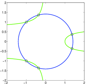
In our first test, we simply take $S={\mathcal{V}}_{\mathbb{R}}(f)$. Since the Hilbert function of $I(S)$ is $1,3,5,6,6,\dots$, we can show that $I(S)$ is generated by $I(S)_{\leq 3}$. A basis for the linear space $I(S)_{\leq 3}$, computed as in § 5, is:

$$G=\left\{\begin{array}[]{l}y^{3}+x^{2}y-2y,~{}xy^{2}-x/2+1/2,\\ x^{3}-3x/2-1/2,~{}x^{2}+y^{2}-2\end{array}\right\}.$$

Using either $f$ or a Gröbner basis for $\langle f\rangle$, e.g.,

$$\{x^{2}+y^{2}-2,~{}2xy^{2}-x+1,~{}2y^{4}-5y^{2}-x+2\},$$ (7)

every $g\in G$ was found to be in $\sqrt[{\mathbb{R}}]{\langle f\rangle}$ showing that $S$ is indeed equal to ${\mathcal{V}}_{\mathbb{R}}(f)$.

Incomplete solution set

Suppose that we take $R={\mathcal{V}}_{\mathbb{R}}(f)\cap\{y\geq 0\}$. Since the Hilbert function of $I(R)$ is $1,3,3,\dots$ and $I(R)_{\leq 1}=\{0\}$, we know that $I(R)$ is generated by three quadratics, approximately

$$G=\left\{\begin{array}[]{l}y^{2}-2.049y-0.18301x+0.86603,\\ xy-0.18301y-0.68301x+1/2\\ x^{2}+0.18301x+2.049y-2.866\end{array}\right\}.$$ (8)

Using $\alpha_{\text{max}}=5$, we were unable to validate that any of the polynomials in $G$ where in $\sqrt[{\mathbb{R}}]{\langle f\rangle}$. In fact, we can show that this is indeed correct since each polynomial in $G$ is nonzero at each of the three points in ${\mathcal{V}}_{\mathbb{R}}(f)\setminus R$.

Semialgebraic condition

We now validate that $R={\mathcal{V}}_{\mathbb{R}}(f)\cap\{y\geq 0\}$ is the complete solution set for the ${\mathcal{A}}$-radical of $\langle f\rangle$ where ${\mathcal{A}}=\{y\geq 0\}$. To that end, we add a slack variable $z$ and consider the system

$$F=\{x^{2}+y^{2}-2,~{}2xy^{2}-x+1,~{}y-z^{2}\}.$$

As described in § 7, we just need to show that each polynomial in $G$ from (8) is contained in $\sqrt[{\mathbb{R}}]{\langle F\rangle}$. Using either $F$ or a Gröbner basis for $\langle F\rangle$, namely (7) together with $y-z^{2}$, we validated that $G\subset\sqrt[{\mathbb{R}}]{\langle F\rangle}$ showing that $R$ is indeed equal to ${\mathcal{V}}_{\mathbb{R}}(f)\cap\{y\geq 0\}$, i.e., $\sqrt[{\mathcal{A}}]{\langle f\rangle}=I(R)$.

8.2 Positive-dimensional components

To illustrate the approach on a system such that the real radical ideal is positive-dimensional, consider the system

$$f=\{xyz,\,z(x^{2}+y^{2}+z^{2}+y),\,y(y+z)\}.$$

The set ${\mathcal{V}}_{\mathbb{C}}(f)$ consists of three lines, two of which are complex conjugates of each other that intersect at the origin and the other is a double line with respect to $f$, and an isolated point. In particular, ${\mathcal{V}}_{\mathbb{R}}(f)$ is the line $y=z=0$ and the isolated point $(0,-1/2,1/2)$. So, we take

$$S=\{(x,0,0)~{}|~{}x\in{\mathbb{C}}\}\cup\{(0,-1/2,1/2)\}\subset\overline{{\mathcal{V}}_{\mathbb{R}}(f)}.$$

To simplify the real computations later, we first replace $f$ with a Gröbner basis for the radical $\sqrt{\langle f\rangle}$, namely

$$f=\{2yz-y,\,2y^{2}+y,\,xy,\,4x^{2}z+4z^{3}+y\}.$$

With the isolated solution, sampling 3 points on the line is enough to compute a basis for $I(S)_{\leq 2}$ which generates $I(S)$:

$$G=\{z^{2}+y/2,\,yz-y/2,\,y^{2}+y/2,\,xz,\,xy,\,y+z\}.$$

Each element in $G$ was shown to belong to $\sqrt[{\mathbb{R}}]{\langle f\rangle}$ with $\alpha\leq 2$.

8.3 Katsura-5 system

As an illustration of our approach on a problem which was solved using the semidefinite characterization of the real radical in [34], we consider the Katsura-5 system as in [34, Ex. 5.4]. The system consists of a linear, say $f_{1}$, and five quadratics, say $f_{2},\dots,f_{6}$, in six variables, namely

$$f=\hbox{\scriptsize$\left\{\begin{array}[]{c}x_{1}+2(x_{2}+x_{3}+x_{4}+x_{5}+x_{6})-1,\\ x_{1}^{2}+2(x_{2}^{2}+x_{3}^{2}+x_{4}^{2}+x_{5}^{2}+x_{6}^{2})-x_{1},\\ 2(x_{1}x_{2}+x_{2}x_{3}+x_{3}x_{4})+x_{4}x_{5}+x_{5}x_{6}-x_{2},\\ x_{2}^{2}+2(x_{1}x_{3}+x_{2}x_{4}+x_{3}x_{5}+x_{4}x_{6})-x_{3},\\ 2(x_{1}x_{4}+x_{2}x_{3}+x_{2}x_{5}+x_{3}x_{6})-x_{4},\\ x_{3}^{2}+2(x_{1}x_{4}+x_{1}x_{5}+x_{1}x_{6})-x_{5}\end{array}\right\}$}.$$

The set ${\mathcal{V}}_{\mathbb{C}}(f)$ consists of $32$ points, $12$ of which lie in ${\mathbb{R}}^{6}$. The set of real solutions, say $S$, is readily computed using homotopy continuation.

The Hilbert function is $1,6,12,12,\dots$ with $I(S)$ being generated by $I(S)_{\leq 2}$. In particular, $I(S)_{\leq 2}$ is a linear space spanned by the linear $f_{1}$ and $15$ quadratics.

Trivially, $f_{1}\in\sqrt[{\mathbb{R}}]{\langle f_{1},\dots,f_{6}\rangle}$ and the quadratics are shown to be in the real radical using $\alpha\leq 2$. This computation validates that ${\mathcal{V}}_{\mathbb{R}}(f)$ consists of $12$ points. Moreover, this data matches that displayed in [34, Table 4].

8.4 Seiler system

As an illustration of our approach on a problem considered in [41, Ex. 5], namely the Seiler system [51]

$$f=\left\{\begin{array}[]{c}x_{3}^{2}+x_{2}x_{3}-x_{1}^{2},\\ x_{1}x_{3}+x_{1}x_{2}-x_{3},\\ x_{2}x_{3}+x_{2}^{2}+x_{1}^{2}-x_{1}\end{array}\right\}.$$

This system does not have a Pommaret basis with respect to the total degree ordering defined by $x_{1}<x_{2}<x_{3}$ [51]. Thus, [41] uses a change of coordinates to overcome this.

Even though $f$ consists of $3$ polynomials in $3$ variables, ${\mathcal{V}}_{\mathbb{C}}(f)$ is actually a curve. In particular, $I=\langle f\rangle$ is a one-dimensional prime ideal, i.e., $I=\sqrt{I}$ and ${\mathcal{V}}_{\mathbb{C}}(I)$ is an irreducible curve. Hence, we know that $I=\sqrt[{\mathbb{R}}]{I}$ if we can compute a real point $x\in{\mathcal{V}}_{\mathbb{R}}(I)$ which is smooth with respect to $f$, i.e., the rank of $Jf(x)$ is $2$.

To that end, we utilize a gradient descent homotopy [21]. We took $y=(1,-3/2,3/4)$ and considered the homotopy

$$H(x,\lambda,t)=\left[\begin{array}[]{c}f(x)-t\cdot f(y)\\ \lambda_{0}(x-y)+\lambda_{1}\nabla f_{1}(x)+\lambda_{2}\nabla f_{2}(x)+\lambda_{3}\nabla f_{3}(x)\end{array}\right]$$

where $\lambda\in{\mathbb{P}}^{3}$. Starting at $x=y$ and $\lambda=[1,0,0,0]\in{\mathbb{P}}^{3}$ when $t=1$, we obtain a point, which is approximately $(0.7009,-0.2504,-0.5868)$, that lies on ${\mathcal{V}}_{\mathbb{R}}(f)$ and is indeed a smooth point on ${\mathcal{V}}_{\mathbb{C}}(f)$. Hence, the isosingular set of this point with respect to $f$ is ${\mathcal{V}}_{\mathbb{C}}(f)$ showing that $I=\sqrt[{\mathbb{R}}]{I}$.

8.5 An energy landscape

Our final example aims to compute the real critical points of the energy landscape of the two-dimensional nearest-neighbor $\phi^{4}$ model on a $3\times 3$ grid as in [17, 45]. We label the nodes $1,\dots,9$ with Figure 2 showing the coupling between the nodes. Let $N(i)$ denote the four nearest neighbors of node $i$, e.g., $N(1)=\{2,3,4,7\}$. After selecting various parameters for this model, we consider the potential energy

$$\mbox{$\displaystyle V(x)=\sum_{i=1}^{9}\left[\frac{1}{40}x_{i}^{4}-x_{i}^{2}+\frac{1}{4}\sum_{j\in N(i)}(x_{i}-x_{j})^{2}\right]$}.$$

The system defining the critical points is $f=\nabla V$ so that

$$f_{i}=\frac{1}{10}x_{i}^{3}-2x_{i}+\sum_{j\in N(i)}(x_{i}-x_{j})$$

Figure 2: Nearest-neighbor coupling for a $3\times 3$ grid of nodes.

The system $f$ is a Gröbner basis and the set ${\mathcal{V}}_{\mathbb{C}}(f)$ consists of $3^{9}=\mbox{19,683}$ points. However, when searching for real stationary points, one only obtains $3$ points, namely

$$S=\{(0,0,0,0,0,0,0,0,0),~{}\pm(w,w,w,w,w,w,w,w,w)\}$$

where $w=\sqrt{20}\approx 4.4721$. Hence, $I(S)$ is generated by

$$G=\{x_{1}(x_{1}^{2}-20),x_{2}-x_{1},\dots,x_{9}-x_{1}\}.$$

All nine basis elements were found to be in $\sqrt[{\mathbb{R}}]{\langle f\rangle}$ with $\alpha=1,2,\dots,2$, respectively. Therefore, $S={\mathcal{V}}_{\mathbb{R}}(f)$, i.e., the energy landscape $V$ has exactly three real critical points.

9 Conclusion

By combining numerical algebraic geometry with sums of squares programming, we have produced a method for certifying that a set of polynomials generate the real radical. The set of polynomials arises from the generators of a set $S$ which is contained in the Zariski closure of the set of real solutions. As first considered in [15], combining numerical algebraic geometry and semidefinite programming can improve the efficiency of computations and produce new approaches, in particular for computing and analyzing the set of real solutions of a system of polynomial equations.

References

- [1] P. Aubry, F. Rouillier, and M. Safey El Din. Real solving for positive dimensional systems. Journal of Symbolic Computation, 34(6):543–560, 2002.
- [2] P. Aubry, F. Rouillier, and M. Safey El Din. Real solving for positive dimensional systems. J. Symbolic Comput., 34(6):543–560, 2002.
- [3] B. Bank, M. Giusti, J. Heintz, and G.M. Mbakop. Polar varieties and efficient real elimination. Mathematische Zeitschrift, 238(1):115–144, 2001.
- [4] D.J. Bates, D.A. Brake, J.D. Hauenstein, A.J. Sommese, and C.W. Wampler. On computing a cell decomposition of a real surface containing infinitely many singularities. In Mathematical Software – ICMS 2014, volume 8592 of Lecture Notes in Computer Science, pages 246–252. Springer, 2014.
- [5] D.J. Bates, J.D. Hauenstein, T.M. McCoy, C. Peterson, and A.J. Sommese. Recovering exact results from inexact numerical data in algebraic geometry. Experimental Mathematics, 22(1):38–50, 2013.
- [6] D.J. Bates, J.D. Hauenstein, C. Peterson, and A.J. Sommese. A numerical local dimension test for points on the solution set of a system of polynomial equations. SIAM Journal on Numerical Analysis, 47(5):3608–3623, 2009.
- [7] D.J. Bates, J.D. Hauenstein, A.J. Sommese, and C.W. Wampler. Numerically solving polynomial systems with Bertini, volume 25. SIAM, 2013.
- [8] E. Becker and R. Neuhaus. Computation of real radicals of polynomial ideals. In Computational algebraic geometry, pages 1–20. Springer, 1993.
- [9] E. Becker and T. Wörmann. Radical computations of zero-dimensional ideals and real root counting. Mathematics and Computers in Simulation, 42(4):561–569, 1996.
- [10] C. Beltrán and A. Leykin. Robust certified numerical homotopy tracking. Found. Comput. Math., 13(2):253–295, 2013.
- [11] G.M. Besana, S. DiRocco, J.D. Hauenstein, A.J. Sommese, and C.W. Wampler. Cell decomposition of almost smooth real algebraic surfaces. Numerical Algorithms, 63(4):645–678, 2013.
- [12] D.A. Brake, D.J. Bates, W. Hao, J.D. Hauenstein, A.J. Sommese, and C.W. Wampler. Bertini_real: Software for one-and two-dimensional real algebraic sets. In Mathematical Software–ICMS 2014, pages 175–182. Springer, 2014.
- [13] D.A. Brake, J.D. Hauenstein, and A.J. Sommese. Numerical local irreducible decomposition. To appear in LNCS.
- [14] E.K.P. Chong and S.H. Zak. An introduction to optimization, volume 76. John Wiley & Sons, 2013.
- [15] D. Cifuentes and P.A. Parrilo. Sampling algebraic varieties for sum of squares programs. arXiv:1511.06751, 2015.
- [16] J.P.K. Doye and D.J. Wales. Saddle points and dynamics of lennard-jones clusters, solids, and supercooled liquids. The Journal of Chemical Physics, 116(9), 2002.
- [17] R. Franzosi, L. Casetti, L. Spinelli, and M. Pettini. Topological aspects of geometrical signatures of phase transitions. Phys. Rev. E, 60:R5009–R5012, Nov 1999.
- [18] P. Gianni, B. Trager, and G. Zacharias. Gröbner bases and primary decomposition of polynomial ideals. Journal of Symbolic Computation, 6(2):149–167, 1988.
- [19] A. Griewank and M. R. Osborne. Newton’s method for singular problems when the dimension of the null space is . SIAM J. Numer. Anal., 18(1):145–149, 1981.
- [20] A. Griewank and M. R. Osborne. Analysis of Newton’s method at irregular singularities. SIAM J. Numer. Anal., 20(4):747–773, 1983.
- [21] Z.A. Griffin and J.D. Hauenstein. Real solutions to systems of polynomial equations and parameter continuation. Adv. Geom., 15(2):173–187, 2015.
- [22] Z.A. Griffin, J.D. Hauenstein, C. Peterson, and A.J. Sommese. Numerical computation of the Hilbert function and regularity of a zero dimensional scheme. In Connections between algebra, combinatorics, and geometry, volume 76 of Springer Proc. Math. Stat., pages 235–250. Springer, New York, 2014.
- [23] J.D. Hauenstein. Numerically computing real points on algebraic sets. Acta applicandae mathematicae, 125(1):105–119, 2013.
- [24] J.D. Hauenstein, I. Haywood, and A.C. Liddell, Jr. An a posteriori certification algorithm for newton homotopies. In Proceedings of the 39th International Symposium on Symbolic and Algebraic Computation, ISSAC ’14, pages 248–255, New York, NY, USA, 2014. ACM.
- [25] J.D. Hauenstein and A.C. Liddell Jr. Certified predictor-corrector tracking for newton homotopies. Journal of Symbolic Computation, 74:239 – 254, 2016.
- [26] J.D. Hauenstein, A.J. Sommese, and C.W. Wampler. Regenerative cascade homotopies for solving polynomial systems. Appl. Math. Comput., 218(4):1240–1246, 2011.
- [27] J.D. Hauenstein and F. Sottile. Algorithm 921: alphaCertified: certifying solutions to polynomial systems. ACM Transactions on Mathematical Software (TOMS), 38(4):28, 2012.
- [28] J.D. Hauenstein and C.W. Wampler. Isosingular sets and deflation. Found. Comput. Math., 13(3):371–403, 2013.
- [29] I. Janovitz-Freireich, B. Mourrain, L. Rónyai, and Á. Szántó. On the computation of matrices of traces and radicals of ideals. Journal of Symbolic Computation, 47(1):102–122, 2012.
- [30] C.T. Kelley. Iterative methods for optimization, volume 18 of Frontiers in Applied Mathematics. Society for Industrial and Applied Mathematics (SIAM), Philadelphia, PA, 1999.
- [31] C.T. Kelley. Solving nonlinear equations with Newton’s method. SIAM, Philadelphia, 2003.
- [32] T. Krick and A. Logar. An algorithm for the computation of the radical of an ideal in the ring of polynomials. In Applied algebra, algebraic algorithms and error-correcting codes, pages 195–205. Springer, 1991.
- [33] J.B. Lasserre, M. Laurent, B. Mourrain, P. Rostalski, and P. Trébuchet. Moment matrices, border bases and real radical computation. Journal of Symbolic Computation, 51:63–85, 2013.
- [34] J.B. Lasserre, M. Laurent, and P. Rostalski. Semidefinite characterization and computation of zero-dimensional real radical ideals. Foundations of Computational Mathematics, 8(5):607–647, 2008.
- [35] J.B. Lasserre, M. Laurent, and P. Rostalski. A prolongation–projection algorithm for computing the finite real variety of an ideal. Theoretical Computer Science, 410(27):2685–2700, 2009.
- [36] J.B. Lasserre, M. Laurent, and P. Rostalski. A unified approach to computing real and complex zeros of zero-dimensional ideals. In Emerging applications of algebraic geometry, pages 125–155. Springer, 2009.
- [37] M. Laurent and P. Rostalski. The approach of moments for polynomial equations. In Handbook on Semidefinite, Conic and Polynomial Optimization, pages 25–60. Springer, 2012.
- [38] B. Lesieutre and D. Wu. An efficient method to locate all the load flow solutions – revisited. In 53rd Annual Allerton Conf. Commun., Control, and Comput., Sept. 29 - Oct. 2 2015.
- [39] Y. Lu, D.J. Bates, A.J. Sommese, and C.W. Wampler. Finding all real points of a complex curve. In Algebra, Geometry and their Interactions, volume 448 of Contemporary Mathematics, pages 183–205, 2007.
- [40] W. Ma and J.S. Thorp. An efficient algorithm to locate all the load flow solutions. IEEE Transactions on Power Systems, 8(3):1077–1083, Aug 1993.
- [41] Y. Ma, C. Wang, and L. Zhi. A certificate for semidefinite relaxations in computing positive-dimensional real radical ideals. Journal of Symbolic Computation, 2014.
- [42] M. Marshall. Positive polynomials and sums of squares, volume 146 of Mathematical Surveys and Monographs. American Mathematical Society, Providence, RI, 2008.
- [43] D. Mehta, T. Chen, J.D. Hauenstein, and D.J. Wales. Communication: Newton homotopies for sampling stationary points of potential energy landscapes. The Journal of Chemical Physics, 141(12):121104, 2014.
- [44] D. Mehta, T. Chen, J.W.R Morgan, and D.J. Wales. Exploring the potential energy landscape of the Thomson problem via Newton homotopies. The Journal of Chemical Physics, 142(19):194113, 2015.
- [45] D. Mehta, J.D. Hauenstein, and M. Kastner. Energy-landscape analysis of the two-dimensional nearest-neighbor model. Phys. Rev. E, 85:061103, Jun 2012.
- [46] R. Neuhaus. Computation of real radicals of polynomial ideals – ii. Journal of Pure and Applied Algebra, 124(1):261–280, 1998.
- [47] A. Papachristodoulou, J. Anderson, G. Valmorbida, S. Prajna, P. Seiler, and P.A. Parrilo. SOSTOOLS: Sum of squares optimization toolbox for MATLAB. http://arxiv.org/abs/1310.4716, 2013. Available from http://www.eng.ox.ac.uk/control/sostools, http://www.cds.caltech.edu/sostools and http://www.mit.edu/~parrilo/sostools.
- [48] F. Rouillier, M.-F. Roy, and M. Safey El Din. Finding at least one point in each connected component of a real algebraic set defined by a single equation. J. Complexity, 16(4):716–750, 2000.
- [49] M. Safey El Din and É. Schost. Polar varieties and computation of one point in each connected component of a smooth real algebraic set. In Proceedings of the 2003 international symposium on Symbolic and algebraic computation, pages 224–231. ACM, 2003.
- [50] A. Seidenberg. A new decision method for elementary algebra. Ann. of Math. (2), 60:365–374, 1954.
- [51] W. Seiler. Involution – the formal theory of differential equations and its applications in computer algebra and numerical analysis. Habilitation thesis. University of Mannheim, 2002.
- [52] S. Smale. Newton’s method estimates from data at one point. Springer, 1986.
- [53] A.J. Sommese and J. Verschelde. Numerical homotopies to compute generic points on positive dimensional algebraic sets. J. Complexity, 16(3):572–602, 2000. Complexity theory, real machines, and homotopy (Oxford, 1999).
- [54] A.J. Sommese and C.W. Wampler. Numerical algebraic geometry. In The mathematics of numerical analysis (Park City, UT, 1995), volume 32 of Lectures in Appl. Math., pages 749–763. Amer. Math. Soc., Providence, RI, 1996.
- [55] A.J. Sommese and C.W. Wampler, II. The numerical solution of systems of polynomials arising in engineering and science. World Scientific Publishing Co. Pte. Ltd., Hackensack, NJ, 2005.
- [56] S.J. Spang. On the computation of the real radical. PhD thesis, Thesis, Technische Universität Kaiserslautern, 2007.
- [57] G. Stengle. A nullstellensatz and a positivstellensatz in semialgebraic geometry. Math. Ann., 207:87–97, 1974.
- [58] B. Xia and L. Yang. An algorithm for isolating the real solutions of semi-algebraic systems. Journal of Symbolic Computation, 34(5):461–477, 2002.
- [59] G. Zeng. Computation of generalized real radicals of polynomial ideals. Science in China Series A: Mathematics, 42(3):272–280, 1999.