Probing CP violation in $e^{+}e^{-}$ production of the Higgs boson and toponia

Abstract

We study the CP violation in the Higgs boson and toponia production process at the ILC where the toponia are produced near the threshold. With the approximation that the production vertex of the Higgs boson and toponia is contact, and neglecting the P-wave toponia, we analytically calculated the density matrix for the production and decay of the toponia. Under these assumptions, the production spectrum of the toponia is solely determined by the spin quantum number, therefore the toponia can be either singlet or triplet. We find that the production rate of the singlet toponium is highly suppressed, and behaves just like the production of a P-wave toponia. In the case of the triplet toponium, three completely independent CP observables, namely azimuthal angles of lepton and anti-lepton in the toponium rest-frame as well as their sum, are predicted based on our analytical results, and checked by using the tree-level event generator. The non-trivial correlations come from the longitudinal-transverse interferences for the azimuthal angles of leptons, and the transverse-transverse interference for their sum. These three observables are well defined at the ILC, where the rest frame of the toponium can be reconstructed directly. Furthermore, the QCD-strong corrections, which are important near the threshold region, are also studied with the approximation of spin-independent QCD-Coulomb potential. While the total cross section is enhanced, the spin correlations predicted in this paper are not affected.

I Introduction

Precise measurements of various physical properties of the observed Higgs particle $h(125)$ ATLAS:Higgs2012 ; CMS:Higgs2012 are the most important and urgent tasks in the elementary particle physics. Of particular interest is the property under the charge conjugation and the parity transformation, which is called the CP property. In general, the mass eigenstate $h(125)$ can be either CP eigenstate or a mixture of CP-even and CP-odd scalar particles. While only one CP-even scalar particle is predicted in the standard model (SM), many of its extensions not only modify the Higgs couplings to gauge bosons and fermions, but also predict additional scalar and pseudo-scalar particles. Therefore decisive measurement of the CP property of $h(125)$ can tell directly whether the observed boson is the Higgs boson in the SM, or it is described by the model beyond the SM. The CP property of $h(125)$ has been investigated experimentally by both ATLAS and CMS collaborations ATLAS:Higgs:CP2013 ; CMS:Higgs:CP2013 ; CMS:Higgs:CP4l2014 through the decays into vector boson pairs, and the experimental results disfavor the pure CP-odd hypothesis by nearly $3\sigma$. However a large CP mixing has not been excluded yet Kobakhidze:2014gqa ; Ellis:2013 ; Abe:2014 ; Nishiwaki:2014 ; Klevtsov:2014 ; Bolognesi:2012 ; Brod:2013 ; Shu:2013 ; Dolan:2014 ; Chen:2014-1 ; Chen:2014-2 ; Bishara:2014 ; Korchin:2013 ; Bernreuther:2010 ; Plehn:2002 ; Aquila:1989-1 ; Aquila:1989-2 ; Harnik:2013 ; Bower:2002 ; Desch:2003 ; Berge:2008 ; Berge:2009 ; Berge:2011 ; Berge:2013 ; Hagiwara:2015 . The reasons are twofold: first, the CP-even coupling of Higgs to the $Z$ boson pair appears at the tree level while the CP-odd coupling appears only at the loop level; second, the branching ratio to the $ZZ^{\star}$ is small.

Theoretically, the CP property of $h(125)$ can also be measured by studying the spin correlations of the two jets in the $pp\rightarrow hjj$ process Plehn:2002 , and the spin correlation in the $h\rightarrow\tau\tau$ channel Aquila:1989-1 ; Aquila:1989-2 ; Harnik:2013 ; Bower:2002 ; Desch:2003 ; Berge:2008 ; Berge:2009 ; Berge:2011 ; Berge:2013 . For the process $pp\rightarrow hjj$, the QCD backgrounds can significantly reduce the signal significance Plehn:2002 , even through the jet-matching technique can be useful to select out the signals Hagiwara:2015 . On the other hand, the CP properties of the Higgs boson can be investigated by using the Higgs coupling to top quarks which is the largest Yukawa coupling in the SM, $y_{t}\sim\mathcal{O}(1)$. The ATLAS group have studied the $t\bar{t}h$ production with an integrated luminosity of $20.3{\rm fb}^{-1}$, and set a $95\%{\rm C.L.}$ limit on the cross section $\sigma_{t\bar{t}h}<4.1\sigma_{t\bar{t}h}^{SM}$. However, the information on the CP properties of the top-Higgs Yukawa coupling is still lacking. In Ref. Kobakhidze:2014gqa , the authors shown that the CP mixing parameter is limited in the range $\xi_{htt}<0.6\pi$. In Refs. Ellis:2013 ; Abe:2014 ; Nishiwaki:2014 constraints on the CP-odd $htt$ coupling is studied by using the LHC run-I data through the $hgg$ and $h\gamma\gamma$ couplings. These constraints are not strong, and still allowing a wide range of the CP-mixing angles. In Ref. Klevtsov:2014 , a strong constraint on the CP-odd $htt$ coupling is derived by using the constraints on electric dipole moments for several nucleus. However, this constraint is obtained under the assumption that the CP-odd $htt$ coupling is only the source of CP violation, which means there is no contribution from heavier Higgs bosons, sparticle, electron-Higgs CP-odd couplings, etc. . If there are other sources of CP violation and there is a cancelation between them, the constraint can be weakened.

As well, there have also appeared many papers devoted to find optimized CP observables at hadron colliders Kolodziej:2015qsa ; Buckley:2015 ; Casolino:2015cza ; Brod:2013cka ; Ellis:2013yxa ; Demartin:2014fia ; Boudjema:2015nda ; Nishiwaki:2013cma ; He:2014xla and lepton colliders Bhupal:2008 ; Godbole:2007 ; Godbole:2011 ; Ananthanarayan:2014eea ; Ananthanarayan:2013cia . The simplest one requires the reconstruction of the top- and anti-top-quark momenta from their decay products which is difficult to be measured accurately even at lepton colliders. In principle, one can construct CP-odd observables by replacing the top- and anti-top-quark momenta by the momenta of the $b$ and $\bar{b}$-jets from the $t$ and $\bar{t}$ decays, respectively. However, the sensitivity to the CP violating effects gets diluted in this partial reconstruction. It has also been pointed out that the different phase-space distributions for scalar and pseudo-scalar Higgs boson production rates can be used to determine the CP properties of the $t\bar{t}h$ coupling. In Ref. Bhupal:2008 , the authors have demonstrated that the CP properties of Higgs can be assessed by measuring just the total cross section and the top-quark polarization. However, these two observables are CP-even, hence only proportional to the square of the CP-odd coupling. Furthermore, the ratio of the production rates for pseudo-scalar and for scalar is very small unless $\sqrt{s}\gg 1~{}{\rm TeV}$ where the chiral limit is recovered. Therefore, the experimental sensitivities of these observables are not as good as enough to probe small CP-odd coupling. To pin down the CP property of the Higgs boson, true CP-odd observables, which is linearly proportional to the CP-odd coupling are really required. The up-down asymmetry of the momentum direction of the anti-top quark with respect to the top-quark-electron plane is an example of such an observable Godbole:2007 ; Godbole:2011 . However, the asymmetry is due to the interferences between the amplitudes involving the $t\bar{t}h$ vertex and those involving the $hZZ$ vertex. It has been shown that the latter contribution is very small, amounting to only a few percent for $\sqrt{s}\leq 1~{}{\rm TeV}$ Bhupal:2008 . Therefore only about 5% asymmetry can be observed at the largest Godbole:2007 ; Godbole:2011 .

In this paper, we study the density matrix for the $e^{+}e^{-}$ production of the Higgs boson and toponia analytically, and propose new CP-odd observables for the measurement of the CP property of the Higgs boson at the ILC with $\sqrt{s}=500~{}{\rm GeV}$Ananthanarayan:2013cia ; Ananthanarayan:2014eea ; ILC:scenarios ; ILC1 ; ILC2 . In this energy region, the strong-interaction Coulomb force is known to be important to calculate the total production rate. Because the P-wave $t\bar{t}$ production is heavily suppressed, we focus on the S-wave toponia production. The contents of this paper is organized as follows. In Sec. II we discuss the effective $t\bar{t}$ production vertex and the spectrum of the toponia in the $e^{+}e^{-}\rightarrow t\bar{t}h$ process. In Sec. III we present the helicity amplitudes for the S-wave toponia productions and their decays. In Sec. IV we study the QCD bound-state effects for the $t\bar{t}$ system. In Sec. V we give the numerical results based on the tree-level event generator, and discuss the CP asymmetries from leptonic observables. Finally, discussions and conclusions are given in Sec. VI.

II Effective $t-\bar{t}-h$ vertex

In this section we study how the $t\bar{t}h$ interactions affect the $t\bar{t}$ system production near the threshold. We assume that the observed Higgs particle $h(125)$ is a mixture of CP-even ($H$) and CP-odd ($A$) particles,

$$h = H\cos\xi+A\sin\xi\,,$$ (1)

where $\xi$ is the Higgs mixing angle which is assumed to be real. For simplicity, we further assume that the Yukawa interactions are CP conserving,

$$\mathcal{L}_{\rm int.} = -g_{Hff}\bar{\psi}_{f}\psi_{f}H-ig_{Aff}\bar{\psi}_{f}\gamma^{5}\psi_{f}A\,,$$ (2)

such that the source of CP violation is only in the Higgs mixing angle $\xi$ in Eq. (1). The interactions between the mass eigenstate $h(125)$ and the fermion anti-fermion pair are then described by

$$\mathcal{L}_{\rm int.} = -g_{hff}h\big{(}\bar{\psi}_{f}\psi_{f}+i\tan\xi_{hff}\bar{\psi}_{f}\gamma^{5}\psi_{f}\big{)}\,,$$ (3)

where

$$g_{hff} = g_{Hff}\cos\xi\,,~{}~{}~{}~{}\tan\xi_{hff}=\frac{g_{Aff}}{g_{Hff}}\tan\xi\,.$$ (4)

It is worth noting that the effective strengths of the CP-violating $hff$ couplings can be different for each fermion, even if the origin of CP-violation is only in the mixing parameter $\xi$. In this paper, we focus on the $ht\bar{t}$ coupling, and for convenience we use the symbol $g_{h}$ to denote the overall coupling constant $g_{ht\bar{t}}$, i.e. $g_{h}=g_{ht\bar{t}}$. The assumption of the real mixing parameter is valid when CP violation in the Higgs sector is mediated mainly by the interactions with new heavy particles.

For the $s$-channel production of $t\bar{t}$ associated with $h(125)$,

$$e^{-}(k_{1},\sigma_{e})+e^{+}(k_{2},\sigma_{\bar{e}}) \rightarrow t(p_{1},\sigma_{t})+\bar{t}(p_{2},\sigma_{\bar{t}})+h(k),$$ (5)

$h(125)$ can be emitted from either a very virtual top-quark or anti-top quark as shown in Fig. 1.

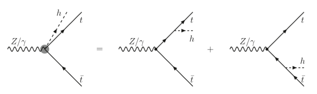
Figure 1: Feynman diagrams which contribute to the $B-ht\bar{t}$ effective vertex (labeled by a big gray dot) in the threshold region.

Even through the Higgs boson can also be produced through the $hBB^{\prime}$ vertexes ($B=Z,\gamma$), the contributions are negligible (a few percent for $\sqrt{s}\leq 1~{}{\rm TeV}$ Bhupal:2008 ) because of the far off-shell propagator of the vector bosons. In principle, CP violation can also appear in these vetrices. However CP violating operators are induced at the one-loop level, and hence hugely suppressed compared to the CP-even operators. Therefore, we do not consider them to simplify the vertex function in this section.

Near the production threshold at $\sqrt{s_{\rm thr.}}=2m_{t}+m_{h}\simeq 471~{}{\rm GeV}$, the $t\bar{t}h$ system is non-relativistic. According to the uncertainty principle, the virtual top and anti-top quarks can propagate only in a distance $\sim 1/(\sqrt{s}-m_{t})$, which is considerably shorter than the Coulomb radius $r_{C}\sim 1/(\alpha_{s}m_{t})$, at which the QCD interactions bound top and anti-top quarks to form the bound states toponia. Therefore treating the whole production vertex as a local interaction should be a good approximation near the threshold. By denoting the vertex of $t\bar{t}$ production from a virtual vector boson $B$ ($B=\gamma,Z$) as $\Gamma_{B}^{\mu}=g_{V}^{Bt\bar{t}}\gamma^{\mu}+g_{A}^{Bt\bar{t}}\gamma^{\mu}\gamma^{5}$, the leading order effective Higgs radiation vertex is given as

$$V^{\mu}(p_{1},p_{2}) = \frac{1}{Q^{2}-2Q\cdot p_{2}}\Gamma_{h}(Q\!\!\!\!/-p\!\!\!/_{2}+m_{t})\Gamma^{\mu}_{B}-\frac{1}{Q^{2}-2Q\cdot p_{1}}\Gamma^{\mu}_{B}(Q\!\!\!\!/-p\!\!\!/_{1}-m_{t})\Gamma_{h},$$ (6)

where $\Gamma_{h}$ is the abbreviation of the $t\bar{t}h$ vertex which is $\Gamma_{h}=g_{h}$ for the pure scalar case and $\Gamma_{h}=g_{h}\tan\xi_{ht\bar{t}}\gamma_{5}$ for the pure pseudo-scalar case, and the kinematical variables are defined as in Fig. 2 with $Q=k_{1}+k_{2}=p_{1}+p_{2}+k$.

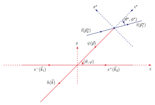
Figure 2: Definitions of the kinematical variables in the $e^{+}e^{-}$ rest frame specified by the axes $x$-$y$-$z$, and the $t\bar{t}$ rest-frame specified by the axes $x^{\star}$-$y^{\star}$-$z^{\star}$. In the $e^{+}e^{-}$ rest-frame, the electron momentum is chosen along the $z$-axis and the $t\bar{t}$ momentum lies in the $x$-$z$ plane with positive $x$-component. In the $t\bar{t}$ rest-frame, the $h$ momentum direction is chosen as the opposite of the $z^{\star}$-axis, and the $y^{\star}$-axis is taken as the same direction as the $y$-axis.

Because both $t\bar{t}$ and $h(125)$ are non-relativistic, the 3-momenta $\vec{p}_{1,2}$ could be neglected in the denominators i.e. $p_{1,2}^{\mu}\approx(m_{t},\vec{0})$. Then the two radiation channels can be combined into a compact form. For convenience, we expand the spinor structure of this vertex by using the Clifford algebra as follows:

$$V^{\mu}(p_{1},p_{2})=\frac{1}{s-2m_{t}\sqrt{s}}\bigg{(}c^{\mu}_{S}+c^{\mu}_{P}\gamma^{5}+c^{\mu\nu}_{V}\gamma_{\nu}+c^{\mu\nu}_{A}\gamma_{\nu}\gamma^{5}+\frac{1}{2}c^{\mu\alpha\beta}_{T}\sigma_{\alpha\beta}\bigg{)}\,,$$ (7)

where we have used $Q^{2}=s$. The expansion coefficients can be calculated easily, as shown in Table 1. The production dynamics are described completely by the vertex function $V^{\mu}(p_{1},p_{2})$ in Eq. (7). Note that the coefficients of the (CP-even) $hBB^{\prime}$ vertexes are not included in Table 1 for the clarity and compactness of the table. These contributions are very small, a few percent for $\sqrt{s}\leq 1~{}{\rm TeV}$ Bhupal:2008 ), and can be easily counted by modifying the coefficients $c_{V}^{\mu\nu}$ and $c_{A}^{\mu\nu}$. Furthermore, the spin correlation which can be used to measure the CP violation effects does not depend on the coefficients of these operators. The magnitudes of these contributions are discussed in the numerical simulation part in Sec. V.

Table 1: The Clifford expansion coefficients in Eq. (7). The $Bt\bar{t}$ ($B=\gamma,Z$) vertex is denoted as $\Gamma_{B}^{\mu}=g_{V}^{Bt\bar{t}}\gamma^{\mu}+g_{A}^{Bt\bar{t}}\gamma^{\mu}\gamma^{5}$. The $ht\bar{t}$ vertex is denoted as $\Gamma_{h}=g_{h}+ig_{h}\tan\xi_{ht\bar{t}}\gamma_{5}$. The momentum $q^{\mu}=p_{1}^{\mu}-p_{2}^{\mu}$ is the relative momentum between the top and anti-top quarks. Note that the coefficients of the (CP-even) $hBB^{\prime}$ vertexes are not included for the clarity and compactness of the table.

$\mathcal{O}_{X}$	Scalar ($\Gamma_{h}=g_{h}$)	Pseudo-Scalar ($\Gamma_{h}=g_{h}\tan\xi_{ht\bar{t}}\gamma_{5}$)
$c^{\mu}_{S}$	$g_{h}\,g_{V}^{Bt\bar{t}}\,q^{\mu}$	$i\,g_{h}\tan\xi_{ht\bar{t}}\,g_{A}^{Bt\bar{t}}(Q^{\mu}+k^{\mu})$
$c^{\mu}_{P}$	$g_{h}\,g_{A}^{Bt\bar{t}}\,(Q^{\mu}+k^{\mu})$	$i\,g_{h}\tan\xi_{ht\bar{t}}\,g_{V}^{Bt\bar{t}}q^{\mu}$
$c^{\mu\nu}_{V}$	$2m_{t}\,g_{h}\,g_{V}^{Bt\bar{t}}\,g^{\mu\nu}$	$0$
$c^{\mu\nu}_{A}$	$2m_{t}\,g_{h}\,g_{A}^{Bt\bar{t}}\,g^{\mu\nu}$	$0$
$c_{T}^{\mu\alpha\beta}$	$ig_{h}\,g_{V}^{Bt\bar{t}}\,\big{[}(Q^{\beta}+k^{\beta})g^{\mu\alpha}-(Q^{\alpha}+k^{\alpha})g^{\mu\beta}\big{]}$; $g_{h}\,g_{A}^{Bt\bar{t}}\,\epsilon^{\alpha\beta\mu\nu}\,q_{\nu}$	$i\,g_{h}\tan\xi_{ht\bar{t}}\,g_{V}^{Bt\bar{t}}\,\epsilon^{\alpha\beta\mu\nu}(Q_{\nu}+k_{\nu})$ ; $g_{h}\tan\xi_{ht\bar{t}}\,g_{A}^{Bt\bar{t}}\,(q^{\alpha}g^{\mu\beta}-q^{\beta}g^{\mu\alpha})$

After the electroweak production of $t\bar{t}h$, the strong interaction between $t\bar{t}$ becomes important. In the threshold region, infinite number of Feynman diagrams whose effects are proportional to the powers of $\alpha_{s}/\beta_{t}\sim\mathcal{O}(1)$ contribute, and their resummation is needed; see Fig. 3.

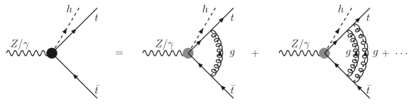
Figure 3: QCD corrections to the effective $V-ht\bar{t}$ vertex in the threshold region. The big black dot indicates the full vertex function after this summation.

After the resummation, the vertex function satisfies an integral equation, the Salpeter-Bethe equation SB:1951 , which describes the formation of bound states in this region. We will discuss it carefully in Sec. IV. Here we would like to classify the possible bound states that can be produced.

Table 2 lists the possible bound states up to P-wave in the spectrum notation for various bi-spinor combinations of spinors $\psi$ and $\varphi$ (see App. VII.1 for our conventions of the spinor wave functions in the Dirac representation), and the corresponding spinor vertex structures in the non-relativistic limit. The spin-singlet state can be produced only by the pseudo-scalar operator $\mathcal{O}_{P}$ and the time component of the axial-vector operator $\mathcal{O}_{V}^{\mu=0}$. All the other operators can generate the spin-triplet state but with different angular momentum.

Table 2: Quantum numbers of the bi-spinors of top and anti-top quarks in the non-relativistic limit in the rest frame of $t\bar{t}$.

Operators	Non-relativistic limit	Quantum state
$\mathcal{O}_{S}=\bar{\psi}\varphi$	$\xi^{{\dagger}}\vec{q}\cdot\vec{\sigma}\eta$	${}^{3}P_{0}$
$\mathcal{O}_{P}=\bar{\psi}\gamma^{5}\varphi$	$\xi^{{\dagger}}\eta$	${}^{1}S_{0}$
$\mathcal{O}_{V}=\bar{\psi}\gamma^{\mu}\varphi$	$(0,\xi^{{\dagger}}\vec{\sigma}\eta)$	${}^{3}S_{1}$
$\mathcal{O}_{A}=\bar{\psi}\gamma^{\mu}\gamma_{5}\varphi$	$(\xi^{{\dagger}}\eta\,,\,\;\xi^{{\dagger}}\vec{q}\times\vec{\sigma}\,\eta)$	$(^{1}S_{0}\,,\,\;^{3}P_{1})$
$\mathcal{O}_{T}=\bar{\psi}\sigma^{0i}\varphi$	$\xi^{{\dagger}}\sigma^{i}\,\eta$	${}^{3}S_{1}$
$\mathcal{O}_{T}=\bar{\psi}\sigma^{ij}\varphi$	$q^{i}\xi^{{\dagger}}\sigma^{j}\,\eta-q^{j}\xi^{{\dagger}}\sigma^{i}\,\eta$	${}^{3}P_{1}$

It should be noted that, all those quantum numbers listed in Table 2 are also affected by the corresponding expansion coefficients, which are tabled in Table 1. In Table 3, we show the possible bound states by combining the coefficients and operators. For the scalar operator $\mathcal{O}_{S}$, both the coefficient and bi-spinor are of P-wave for the scalar Higgs boson. Therefore the $t\bar{t}$ system is D-wave which can be ignored completely. In the case of the pseudo-scalar Higgs boson, the $t\bar{t}$ system is P-wave because the coefficient is S-wave. However, it is still negligible near the threshold region. For the pseudo-scalar operator $\mathcal{O}_{P}$, a singlet toponium can be produced. The coefficient is S-wave for the scalar Higgs boson, while P-wave for the pseudo-scalar Higgs boson. For the vector and axial-vector operators, $\mathcal{O}_{V}$ and $\mathcal{O}_{A}$, only vertexes for scalar Higgs boson production exist. The operator $\mathcal{O}_{V}$ can generate the S-wave triplet toponium, while $\mathcal{O}_{A}$ generates the P-wave triplet toponium. In addition, the axial-vector operator can also generate the S-wave singlet toponium via its time-component. This contribution turns out to be very important, because it is destructive with the contribution of the pseudo-scalar vertex $\mathcal{O}_{P}$, and then makes the total production rate of the singlet toponium highly suppressed. Of particular interest is the production by the tensor operator $\mathcal{O}_{T}$, in which both the bi-spinor and the coefficient contain S-wave and P-wave $t\bar{t}$. Here we discuss only the S-wave contributions. For both scalar and pseudo-scalar Higgs bosons, it is the “electric component” of the tensor operator $\propto\sigma^{0i}$ generating the S-wave toponium.

Table 3: Quantum states of the $t\bar{t}$ and $t\bar{t}h$ systems. The spin and angular momenta are summed first by combining the top and anti-top-quarks system, and then by combining the toponium ($\psi_{t}$) and Higgs system.

Operators	Scalar Higgs		Pseudo-Scalar Higgs
	$(t,\bar{t})$-System	$(\psi_{t},h)$-System	$(t,\bar{t})$-System	$(\psi_{t},h)$-System
$\mathcal{O}_{S}$	${}^{3}D_{1}$	${}^{3}S_{1}$	${}^{3}P_{0}$	${}^{1}P_{1}$
$\mathcal{O}_{P}$	${}^{1}S_{0}$	${}^{1}P_{1}$	${}^{1}P_{1}$	${}^{3}S_{1}$
$\mathcal{O}_{V}$	${}^{3}S_{1}$	${}^{3}S_{1}$	$0$	$0$
$\mathcal{O}_{A}$	${}^{1}S_{0}$	${}^{1}P_{1}$	$0$	$0$
	${}^{3}P_{1}$	${}^{3}S_{1}$	$0$	$0$
$\mathcal{O}_{T}$	${}^{3}S_{1}$	${}^{3}S_{1}$	${}^{3}S_{1}$	${}^{3}P_{1}$
	${}^{3}P_{1}$	${}^{3}P_{1}$	${}^{3}P_{1}$	${}^{3}S_{1}$
	${}^{3}P_{1}$	${}^{3}S_{1}$	${}^{3}P_{1}$	${}^{3}P_{1}$
	${}^{3}D_{1}$	${}^{3}S_{1}$	${}^{3}D_{1}$	${}^{3}S_{1}$

III Helicity amplitudes

In this section we give a formula for the full helicity amplitudes in terms of the toponium angular momentum. Near the threshold the QCD-strong interactions become important. Here we assume the QCD corrections can be completely factorized out, i.e. the strong force is spin-independent; see Sec. IV. In this approximation the full physics could be modeled by using pure electroweak $ht\bar{t}$ production and their decays. Then, the toponium helicity is obtained by the spin projection. The spin projection becomes simple when the relative momentum $q^{\mu}$ between the top and anti-top quarks is neglected. Furthermore neglecting the relative momentum does not lose essential physics as the top and anti-top quarks have large decay width. Therefore, while we calculate the density matrix without the assumption of $|q^{\mu}|\approx 0$, some important results can be discussed under this simplification. In subsection III.1 we give our formalism on the factorization of the QCD correction, as well as that for the spin projection. In subsection III.2 and III.3 we give the helicity amplitudes for the production and decays of toponia. The total helicity amplitude and the CP-odd observables are discussed in subsection III.4.

III.1 Factorization and projection of the helicity amplitudes

The total amplitude for the process $e^{-}+e^{+}\rightarrow h+(\ell\nu_{\bar{\ell}}\bar{b})+(\bar{\ell}\nu_{\ell}b)$ can be written in general as follows:

$$\mathcal{M} = \langle(\ell\nu_{\bar{\ell}}\bar{b})(\bar{\ell}\nu_{\ell}b)h|\mathcal{T}|e^{-}e^{+}\rangle\,.$$ (8)

We focus on the CP violation effects due to the anomalous interaction between the toponia and Higgs boson. This is done by inserting a complete basis of the $t\bar{t}$ resonance states $\psi_{t}$ with quantum number $(J_{\psi_{t}},\lambda_{\psi_{t}})$, then the total helicity amplitude can be written as the product of the production and decay amplitudes of the toponia,

$$\mathcal{M} = \sum_{J_{\psi_{t}},\lambda_{\psi_{t}}}\langle(\ell\nu_{\bar{\ell}}\bar{b})(\bar{\ell}\nu_{\ell}b)|\mathcal{T}_{D}|\psi_{t}(J_{\psi_{t}},\lambda_{\psi_{t}})\rangle\langle\psi_{t}(J_{\psi_{t}},\lambda_{\psi_{t}})h|\mathcal{T}_{P}|e^{-}e^{+}\rangle\,.$$ (9)

However this amplitude cannot be calculated directly in perturbation theory because the $t\bar{t}$ resonances $\psi_{t}$ are composite states. We therefore expand the helicity amplitudes by using the fundamental fields $t$ and $\bar{t}$, and the amplitudes take the following form:

$$\mathcal{M} = \sum_{J_{\psi_{t}},\lambda_{\psi_{t}}}\sum_{\sigma_{t}^{\prime},\sigma_{\bar{t}}^{\prime}}\sum_{\sigma_{t},\sigma_{\bar{t}}}\mathcal{M}_{\psi_{t}}(J_{\psi_{t}},\lambda_{\psi_{t}};\sigma_{t}^{\prime},\sigma_{\bar{t}}^{\prime};\sigma_{t},\sigma_{\bar{t}})\mathcal{M}_{D}(\sigma_{t}^{\prime},\sigma_{\bar{t}}^{\prime})\mathcal{M}_{P}(\sigma_{t},\sigma_{\bar{t}})\,,$$ (10)

where the production, decay and resonance amplitudes are, respectively,

$$\mathcal{M}_{P}(\sigma_{t},\sigma_{\bar{t}}) = \langle t(\sigma_{t})\bar{t}(\sigma_{\bar{t}})h|\mathcal{T}_{P}|e^{-}e^{+}\rangle\,,$$ (11)

$$\mathcal{M}_{D}(\sigma_{t}^{\prime},\sigma_{\bar{t}}^{\prime}) = \langle(\ell\nu_{\bar{\ell}}\bar{b})(\bar{\ell}\nu_{\ell}b)|\mathcal{T}_{D}|t(\sigma_{t}^{\prime})\bar{t}(\sigma_{\bar{t}}^{\prime})\rangle\,,$$ (12)

$$\mathcal{M}_{\psi_{t}}(J_{\psi_{t}},\lambda_{\psi_{t}};\sigma_{t}^{\prime},\sigma_{\bar{t}}^{\prime};\sigma_{t},\sigma_{\bar{t}}) = \langle t(\sigma_{t}^{\prime})\bar{t}(\sigma_{\bar{t}}^{\prime})|\mathcal{T}_{QCD}^{{\dagger}}|\psi_{t}(J_{\psi_{t}},\lambda_{\psi_{t}})\rangle\langle\psi_{t}(J_{\psi_{t}},\lambda_{\psi_{t}})|\mathcal{T}_{QCD}|t(\sigma_{t})\bar{t}(\sigma_{\bar{t}})\rangle\,.$$ (13)

Here both the production and decay processes are electroweak, and the QCD corrections are accounted for in the resonance amplitudes. In order to make our discussions more simple and clear, we use the free $t\bar{t}$ resonance states $\widetilde{\psi}_{t}(J^{\prime}_{\psi},\lambda_{\psi_{t}}^{\prime})$ to separate out the spin degrees of freedom. Then the amplitude for the toponium formation from the top- and anti-top-quarks can be written as

$$\langle\psi_{t}(J_{\psi_{t}},\lambda_{\psi_{t}})|\mathcal{T}_{QCD}|t(\sigma_{t})\bar{t}(\sigma_{\bar{t}})\rangle$$ (14)

$$= \sum_{J^{\prime}_{\psi_{t}},\lambda_{\psi_{t}}^{\prime}}\langle\psi_{t}(J_{\psi_{t}},\lambda_{\psi_{t}})|\mathcal{T}_{QCD}|\widetilde{\psi}_{t}(J^{\prime}_{\psi_{t}},\lambda_{\psi_{t}}^{\prime})\rangle\langle\widetilde{\psi}_{t}(J^{\prime}_{\psi_{t}},\lambda_{\psi_{t}}^{\prime})|\mathcal{O}^{J^{\prime}_{\psi}}_{\lambda_{\psi_{t}}^{\prime}}|t(\sigma_{t})\bar{t}(\sigma_{\bar{t}})\rangle\,,$$

where we have introduced a pure kinematical operator $\mathcal{O}^{J^{\prime}_{\psi}}_{\lambda_{\psi_{t}}^{\prime}}$ to account for the spin correlations of $t\bar{t}$ to $\widetilde{\psi}_{t}$. In general the quantum numbers $(J_{\psi_{t}},\lambda_{\psi_{t}})$ can be different from $(J^{\prime}_{\psi_{t}},\lambda_{\psi_{t}}^{\prime})$ by QCD corrections, for instance when we include the spin-orbital interactions, etc. Here we neglect those spin-dependent corrections, i.e. we take $(J_{\psi_{t}},\lambda_{\psi_{t}})=(J^{\prime}_{\psi_{t}},\lambda_{\psi_{t}}^{\prime})$. Then the resonance amplitudes can be written as

$$\mathcal{M}_{\psi_{t}}(J_{\psi_{t}},\lambda_{\psi_{t}};\sigma_{t}^{\prime},\sigma_{\bar{t}}^{\prime};\sigma_{t},\sigma_{\bar{t}}) = (\mathcal{P}_{\sigma_{t}^{\prime},\sigma_{\bar{t}}^{\prime}}^{J_{\psi_{t}},\lambda_{\psi_{t}}})^{{\dagger}}(\mathcal{P}_{\sigma_{t},\sigma_{\bar{t}}}^{J_{\psi_{t}},\lambda_{\psi_{t}}})\mathcal{K}_{J_{\psi_{t}},\lambda_{\psi_{t}}}\,,$$ (15)

where the factor $\mathcal{K}_{J_{\psi_{t}},\lambda_{\psi_{t}}}$ is defined as the squared renormalization factor which gives the pure QCD corrections,

$$\mathcal{K}_{J_{\psi_{t}},\lambda_{\psi_{t}}} = |\langle\psi(J_{\psi_{t}},\lambda_{\psi_{t}})|\mathcal{T}_{QCD}|\widetilde{\psi_{t}}(J_{\psi_{t}},\lambda_{\psi_{t}})\rangle|^{2}\,,$$ (16)

and the spin projection operator $\mathcal{P}_{\sigma_{t},\sigma_{\bar{t}}}^{J_{\psi},\lambda_{\psi_{t}}}$ is defined as the matrix elements of $\mathcal{O}^{J_{\psi_{t}}}_{\lambda_{\psi_{t}}}$,

$$\mathcal{P}_{\sigma_{t},\sigma_{\bar{t}}}^{J_{\psi},\lambda_{\psi_{t}}} = \langle\widetilde{\psi}(J_{\psi},\lambda_{\psi_{t}})|\mathcal{O}^{J_{\psi}}_{\lambda_{\psi_{t}}}|t(\sigma_{t})\bar{t}(\sigma_{\bar{t}})\rangle\,.$$ (17)

The QCD corrections are discussed in Sec. IV. Let us focus on the spin projection first. In general $J_{\psi_{t}}$ can be any integer. However the production rates of toponium states with higher angular momentum $L$ are suppressed by $\beta_{t}^{L}$ where $\beta_{t}$ is a velocity of top and anti-top quarks in the toponium rest-frame. Therefore, we discuss only the S-wave resonance. Then $\psi_{t}$ can be either spin-singlet or spin-triplet, i.e. $J_{\psi_{t}}=0$ or 1. The corresponding projection operators are defined as follows:

$$\mathcal{O}^{J_{\psi_{t}}=0}_{\lambda_{\psi_{t}}} = \frac{1}{\sqrt{2s_{\psi_{t}}}\sqrt{1-\frac{(m_{t}^{\star 2}-\bar{m}_{t}^{\star 2})^{2}}{s_{\psi_{t}}^{2}}}}\widetilde{\psi}_{t}(\lambda_{\psi_{t}})\bar{t}\gamma^{5}t\,,$$ (18)

$$\mathcal{O}^{J_{\psi_{t}}=1}_{\lambda_{\psi_{t}}} = \frac{1}{\sqrt{2s_{\psi_{t}}}\sqrt{1-\frac{(m_{t}^{\star 2}-\bar{m}_{t}^{\star 2})^{2}}{s_{\psi_{t}}^{2}}}}\widetilde{\psi}_{t}^{\mu}(\lambda_{\psi_{t}})\bar{t}\,\gamma_{\mu}t\,,$$ (19)

where $\sqrt{s_{\psi_{t}}}$, $m_{t}^{\star}$ and $\bar{m}_{t}^{\star}$ are the invariant mass of the toponium, top and anti-top quarks respectively. The normalization factor is chosen such that the spin projection operators are dimensionless (the overall normalization of $\mathcal{M}_{\psi_{t}}$ is fixed by the total QCD correction). With the help of the spin projection operators the total helicity amplitude can be expressed in terms of the toponium production and decay helicity amplitudes as follows:

$$\mathcal{M} = \sum_{J_{\psi_{t}},\lambda_{\psi_{t}}}\mathcal{K}_{J_{\psi_{t}},\lambda_{\psi_{t}}}\widetilde{\mathcal{M}}_{P}(J_{\psi_{t}},\lambda_{\psi_{t}})\widetilde{\mathcal{M}}_{D}(J_{\psi_{t}},\lambda_{\psi_{t}})\,$$ (20)

where the projected production and decay helicity amplitudes are

$$\widetilde{\mathcal{M}}_{P}(J_{\psi_{t}},\lambda_{\psi_{t}}) = \sum_{\sigma_{t},\sigma_{\bar{t}}}\mathcal{P}_{\sigma_{t},\sigma_{\bar{t}}}^{J_{\psi_{t}},\lambda_{\psi_{t}}}\mathcal{M}_{P}(\sigma_{t},\sigma_{\bar{t}})\,,$$ (21)

$$\widetilde{\mathcal{M}}_{D}(J_{\psi_{t}},\lambda_{\psi_{t}}) = \sum_{\sigma_{t}^{\prime},\sigma_{\bar{t}}^{\prime}}(\mathcal{P}_{\sigma_{t}^{\prime},\sigma_{\bar{t}}^{\prime}}^{J_{\psi_{t}},\lambda_{\psi_{t}}})^{{\dagger}}\mathcal{M}_{D}(\sigma_{t}^{\prime},\sigma_{\bar{t}}^{\prime})\,.$$ (22)

In the next two subsections, we study these two helicity amplitudes.

III.2 Production helicity amplitudes

In this subsection we give the helicity amplitudes for the production process of toponia in associated with the Higgs boson. The kinematical variables are defined as (see also the Fig. 2)

$$e^{-}(k_{1},\sigma_{e})+e^{+}(k_{2},\sigma_{\bar{e}}) \rightarrow \widetilde{\psi_{t}}(p;J_{\psi_{t}},\lambda_{\psi_{t}})+h(k)\rightarrow t(p_{1},\sigma_{t})+\bar{t}(p_{2},\sigma_{\bar{t}})+h(k).$$ (23)

The fermion helicities are $\sigma_{i}=\pm 1/2$ for $i=e,\bar{e},t,\bar{t}$. For the spin-singlet toponium $J_{\psi_{t}}=0,\lambda_{\psi_{t}}=0$, and for the spin-triplet toponium $J_{\psi_{t}}=1,\lambda_{\psi_{t}}=0,\pm 1$. In the rest frame of $e^{+}e^{-}$ the particle momenta are given by

$$Q^{\mu} = \sqrt{s}(1,\,0,\,0,\,0)\,,$$ (24a)

$$k_{1}^{\mu} = \dfrac{\sqrt{s}}{2}(1,\,0,\,0,\,1)\,,$$ (24b)

$$k_{2}^{\mu} = \dfrac{\sqrt{s}}{2}(1,\,0,\,0,\,-1)\,,$$ (24c)

$$p^{\mu} = \dfrac{\sqrt{s}}{2}(1+\dfrac{s_{\psi_{t}}-m_{h}^{2}}{s},\,\beta\sin\vartheta\cos\varphi,\,\beta\sin\vartheta\sin\varphi,\,\beta\cos\vartheta)\,,$$ (24d)

$$k^{\mu} = \dfrac{\sqrt{s}}{2}(1-\dfrac{s_{\psi_{t}}-m_{h}^{2}}{s},\,-\beta\sin\vartheta\cos\varphi,\,-\beta\sin\vartheta\sin\varphi,\,-\beta\cos\vartheta)\,.$$ (24e)

Here we use $\sqrt{s}$ to denote the total collision energy, and $\sqrt{s}_{\psi_{t}}$ to denote the invariant mass of the toponium. $\beta$ is a velocity of the Higgs boson and toponium in this frame, which is given as

$$\beta = \sqrt{1+\frac{m_{h}^{4}}{s^{2}}+\frac{s_{\psi_{t}}^{2}}{s^{2}}-\frac{2m_{h}^{2}s_{\psi_{t}}}{s^{2}}-\frac{2m_{h}^{2}}{s}-\frac{2s_{\psi_{t}}}{s}}.$$ (25)

In this frame the leptonic current is give by

$$L_{V}^{\mu}(\lambda_{e}) = -\lambda_{V}{\cal G}_{\lambda_{V}}^{e}\sqrt{2s}\,\varepsilon^{\mu}(\vec{Q}=\vec{0},\lambda_{V})\,,$$ (26)

where $\varepsilon^{\mu}(\vec{Q}=\vec{0},\lambda_{V})$ are given in Eq. (109) and Eq. (110) in the Appendix VII.2 by setting $\theta=0$ and $\phi=0$, $\lambda_{V}=\sigma_{e}-\sigma_{\bar{e}}=\pm 1$ is the helicity of the virtual vector particle $B$ that can be either photon ($B=\gamma$) or $Z$ ($B=Z$); the helicity-dependent form-factor ${\cal G}_{\lambda_{V}}^{e}$ is defined as

$${\cal G}_{\lambda_{V}}^{e}(Q^{2}) = \begin{cases}\dfrac{e}{Q^{2}}&\text{for}\ B=\gamma\\[14.22636pt] -\dfrac{1}{4}\dfrac{(1-\lambda_{V})+4\sin^{2}\theta_{W}}{Q^{2}-m_{Z}^{2}+im_{Z}\Gamma_{Z}}&\text{for}\ B=Z\end{cases}$$ (27)

where the first term stands for the photon pole and the second term stands for the $Z$ pole. The momenta of the toponium, $t$ and $\bar{t}$ in the rest frame of the toponium are given by

$$p^{\star\mu} = \sqrt{s_{\psi}}(1,\,0,\,0,\,0)\,,$$ (28a)

$$p_{1}^{\star\mu} = \dfrac{\sqrt{s_{\psi}}}{2}(1+\frac{m_{t}^{\star 2}-\bar{m}_{t}^{\star 2}}{s_{\psi}},\,\beta_{t}\sin\theta^{\star}\cos\phi^{\star},\,\beta_{t}\sin\theta^{\star}\sin\phi^{\star},\,\beta_{t}\cos\theta^{\star})\,,$$ (28b)

$$p_{2}^{\star\mu} = \dfrac{\sqrt{s_{\psi}}}{2}(1-\frac{m_{t}^{\star 2}-\bar{m}_{t}^{\star 2}}{s_{\psi}},\,-\beta_{t}\sin\theta^{\star}\cos\phi^{\star},\,-\beta_{t}\sin\theta^{\star}\sin\phi^{\star},\,-\beta_{t}\cos\theta^{\star})\,,$$ (28c)

where

$$\beta_{t} = \sqrt{1+\frac{m_{t}^{\star 4}}{s_{\psi}^{2}}+\frac{\bar{m}_{t}^{\star 4}}{s_{\psi}^{2}}-\frac{2m_{t}^{\star 2}\bar{m}_{t}^{\star 2}}{s_{\psi}^{2}}-\frac{2m_{t}^{\star 2}}{s_{\psi}}-\frac{2\bar{m}_{t}^{\star 2}}{s_{\psi}}}.$$ (29)

Let us first calculate the projection operators. Because we discuss only the S-wave toponium, there are only two kinds of projection operators: the spin-singlet and spin-triplet projection operators which correspond to the matrix element of operators $\mathcal{O}_{P}$ and $\mathcal{O}_{V}$. In the rest frame of the toponium we get

$$\mathcal{P}_{\sigma_{t},\sigma_{\bar{t}}}^{J_{\psi_{t}}=0,\lambda_{\psi_{t}}} = -\frac{1}{\sqrt{2}}|\tilde{m}|e^{i\tilde{m}\phi^{\star}}~{}~{}~{}~{}~{}~{}~{}~{}~{}~{}\;\;\,,~{}~{}~{}(\mathcal{P}_{\sigma_{t},\sigma_{\bar{t}}}^{J_{\psi_{t}}=0,\lambda_{\psi_{t}}})^{{\dagger}}=-\frac{1}{\sqrt{2}}|\tilde{m}|e^{-i\tilde{m}\phi^{\star}}$$ (30a)

$$\mathcal{P}_{\sigma_{t},\sigma_{\bar{t}}}^{J_{\psi_{t}}=1,\lambda_{\psi_{t}}} = f(\tilde{m},m)D^{J=1}_{\lambda_{\psi_{t}},m}(\theta^{\star},\phi^{\star})~{},~{}~{}~{}(\mathcal{P}_{\sigma_{t},\sigma_{\bar{t}}}^{J_{\psi_{t}}=1,\lambda_{\psi_{t}}})^{{\dagger}}=f^{\ast}(\tilde{m},m)\widetilde{D}^{J=1}_{m,\lambda_{\psi_{t}}}(\theta^{\star},\phi^{\star})$$ (30b)

where the helicities $m=\sigma_{t}-\sigma_{\bar{t}}$ and $\tilde{m}=\sigma_{t}+\sigma_{\bar{t}}$ are defined along the top-quark momentum direction, and they are related by the Wigner rotation to the helicity states of the toponium along its moving direction. The function $f(\tilde{m},m)$ is defined as follows:

$$f(\tilde{m},m) = \bigg{(}\frac{1}{\sqrt{2}}\tilde{m}\sqrt{1-\beta_{t}^{2}}\,e^{i\tilde{m}\phi^{\star}}-m\bigg{)}\,.$$ (31)

Here we use $\widetilde{D}$ to denote the complex-conjugate-transpose of the Wigner-D functions; see Appendix. As we have worked in the non-relativistic approximation, the relative momentum between top and anti-top quarks is negligible, so the kinematical factor $\beta_{t}$ in the spin-triplet projection operator can be neglected.

The helicity amplitudes of $t\bar{t}h$ production are decomposed by the type of production vertexes. Here we use the notation $\mathcal{M}_{P}(X;\sigma_{t},\sigma_{\bar{t}})$ with $X=S,P,A,V,T$ to denote their contributions, and use subscripts of $X$ to distinguish the contributions of scalar and pseudo-scalar components of the Higgs boson. The operators that can generate the toponium in S-wave are listed in Table 4.

Table 4: Operators which generate the toponium in S-wave

Operators	Scalar Higgs	Pseudo-Scalar Higgs
$\mathcal{O}_{S}$
$\mathcal{O}_{P}$	$\surd$
$\mathcal{O}_{V}$	$\surd$
$\mathcal{O}_{A}$	$\surd$
$\mathcal{O}_{T}$	$\surd$	$\surd$

For the scalar operator, both the scalar and pseudo-scalar components of the Higgs boson start to contribute at P-wave, so there is no relevant contributions. For the pseudo-scalar operator, only the scalar component of the Higgs boson contributes, and the helicity amplitude is

$$\mathcal{M}_{P}(P;\sigma_{t},\sigma_{\bar{t}}) = -\lambda_{V}{\cal G}_{\lambda_{V}}^{e}g_{h}g_{A}s\sqrt{s_{\psi_{t}}}X_{P}|\tilde{m}|e^{-i\tilde{m}\phi^{\star}}\widetilde{D}^{J=1}_{0\lambda_{V}}(\vartheta,\varphi)\,,$$ (32)

where the kinematical factor

$$X_{P} = \frac{\beta}{\sqrt{2}}\sqrt{1-\frac{(m_{t}^{\star 2}-\bar{m}_{t}^{\star 2})^{2}}{s_{\psi}^{2}}}\,,$$ (33)

which is consistent with our previous explanation in Sec. II that the pseudo-scalar operator can only generate the P-wave state of the singlet toponium and Higgs boson. This is also true for the axial-vector operator. The helicity amplitude is similar with $\mathcal{M}_{P}(P;\sigma_{t},\sigma_{\bar{t}})$,

$$\mathcal{M}_{P}(A;\sigma_{t},\sigma_{\bar{t}}) = \lambda_{V}{\cal G}_{\lambda_{V}}^{e}g_{h}g_{A}s\sqrt{s_{\psi_{t}}}X_{A}|\tilde{m}|e^{-i\tilde{m}\phi^{\star}}\widetilde{D}^{J=1}_{m\lambda_{V}}(\vartheta,\varphi)$$ (34)

where the kinematical factor is

$$X_{A} = \frac{\beta}{\sqrt{2}}\sqrt{\frac{4m_{t}^{2}}{s_{\psi_{t}}}}\sqrt{1-\frac{(m_{t}^{\star 2}-\bar{m}_{t}^{\star 2})^{2}}{s_{\psi_{t}}^{2}}}\,.$$ (35)

The important thing is that the contributions of pseudo-scalar and axial vector operators are destructive. Because only the pseudo-scalar and axial vector operators generate the singlet toponium, therefore the total helicity amplitude for the singlet toponium production is just the sum of these two contributions. It is proportional to $1-\sqrt{4m_{t}^{2}/s_{\psi_{t}}}$, and thus negligible near the threshold.

The triplet toponium can be produced through the vector and tensor operators. The helicity amplitude for the vector operator is

$$\mathcal{M}_{P}(V;\sigma_{t},\sigma_{\bar{t}}) = \sum_{\lambda_{\psi_{t}}^{\prime}}\lambda_{V}{\cal G}_{\lambda_{V}}^{e}g_{h}g_{V}s\sqrt{s_{\psi_{t}}}X_{V}\widetilde{D}^{J=1}_{\lambda_{\psi_{t}}^{\prime}\lambda_{V}}(\vartheta,\varphi)f^{\ast}(\tilde{m},m)\widetilde{D}^{J=1}_{m\lambda_{\psi_{t}}^{\prime}}(\theta^{\star},\phi^{\star})\,.$$ (36)

Here the helicity $\lambda_{\psi_{t}}^{\prime}$ is quantized along the moving direction of the toponium in the $e^{+}e^{-}$ rest-frame, and related to $\lambda_{\psi_{t}}$ by the Wigner rotations after spin projection. The kinematical factor is

$$X_{V} = 2\sqrt{\frac{4m_{t}^{2}}{s}}\sqrt{1-\frac{(m_{t}^{\star 2}-\bar{m}_{t}^{\star 2})^{2}}{s_{\psi}^{2}}}\,.$$ (37)

This is a S-wave production, and can be represented by an effective operator $h\psi_{t}^{\mu}B_{\mu}$, where $B=\gamma,Z$. The contribution from the tenser operator is also of S-wave production, and can be represented by an effective operator $hF_{\psi_{t}\mu\nu}F_{B}^{\mu\nu}$, where $F_{B}^{\mu\nu}=\partial^{\mu}B^{\nu}-\partial^{\nu}B^{\mu}$ is the field strength tensor. The corresponding helicity amplitude is

$$\mathcal{M}_{P}(T_{S};\sigma_{t},\sigma_{\bar{t}}) = \sum_{\lambda_{\psi_{t}}^{\prime}}\lambda_{V}{\cal G}_{\lambda_{V}}^{e}g_{h}g_{V}s\sqrt{s_{\psi_{t}}}X_{T_{S}}\widetilde{D}^{J=1}_{\lambda_{\psi_{t}}^{\prime}\lambda_{V}}(\vartheta,\varphi)f^{\ast}(\tilde{m},m)\widetilde{D}^{J=1}_{m\lambda_{\psi_{t}}^{\prime}}(\theta^{\star},\phi^{\star})\,,$$ (38)

where the kinematical factor is

$$X_{T_{S}} = 2\sqrt{\frac{s}{s_{\psi}}}\bigg{(}1-\frac{m_{h}^{2}}{s}\bigg{)}\sqrt{1-\frac{(m_{t}^{\star 2}-\bar{m}_{t}^{\star 2})^{2}}{s_{\psi}^{2}}}\,.$$ (39)

In the above calculations we have neglected a contribution of the D-wave production which is proportional to $\beta^{2}$. Apart from the kinematical factor, the rest is completely the same as the contribution of the vector operator $\mathcal{M}_{P}(V;\sigma_{t},\sigma_{\bar{t}})$. These two contributions are constructive, and hence make the triplet production rate dominant. Furthermore, the pseudo-scalar component of the Higgs boson also contributes in the S-wave toponium production via the tensor operator. However, the overall production is of P-wave. The corresponding effective operator can be written as $h\widetilde{F}_{\psi_{t}\mu\nu}F_{B}^{\mu\nu}$, where $\widetilde{F}_{B}^{\mu\nu}=1/2\epsilon_{\mu\nu\alpha\beta}F_{B}^{\alpha\beta}$ is the dual strength tensor of the field $B$. The helicity amplitude for the tensor operator is,

$$\mathcal{M}_{P}(T_{P};\sigma_{t},\sigma_{\bar{t}}) = -\sum_{\lambda_{\psi_{t}}^{\prime}}i\lambda_{V}{\cal G}_{\lambda_{V}}^{e}\epsilon_{h}g_{V}s\sqrt{s_{\psi}}X_{T_{P}}\widetilde{D}^{J=1}_{\lambda_{\psi_{t}}^{\prime}\lambda_{V}}(\vartheta,\varphi)f^{\ast}(\tilde{m},m)\lambda_{\psi_{t}}^{\prime}\widetilde{D}^{J=1}_{m\lambda_{\psi_{t}}^{\prime}}(\theta^{\star},\phi^{\star})\,,$$ (40)

where the kinematical factor is

$$X_{T_{P}} = 2\beta\sqrt{\frac{s}{s_{\psi}}}\sqrt{1-\frac{(m_{t}^{\star 2}-\bar{m}_{t}^{\star 2})^{2}}{s_{\psi}^{2}}},$$ (41)

and $\epsilon_{h}=g_{h}\tan\xi_{ht\bar{t}}$.

Now we can obtain the projected helicity amplitudes. For the pseudo-scalar and axial vector operators the projected helicity amplitudes are similar with each other;

$$\widetilde{\mathcal{M}}_{P}(P;J_{\psi_{t}}=0) = \sqrt{2}\lambda_{V}{\cal G}_{\lambda_{V}}^{e}g_{h}g_{A}s\sqrt{s_{\psi_{t}}}\beta\widetilde{D}^{J=1}_{0\lambda_{V}}(\vartheta,\varphi)\,.$$ (42)

$$\widetilde{\mathcal{M}}_{P}(A;J_{\psi_{t}}=0) = -\sqrt{2}\lambda_{V}{\cal G}_{\lambda_{V}}^{e}g_{h}g_{A}s\sqrt{s_{\psi_{t}}}\beta\sqrt{\frac{4m_{t}^{2}}{s_{\psi_{t}}}}\widetilde{D}^{J=1}_{0\lambda_{V}}(\vartheta,\varphi)\,.$$ (43)

Because only these two operators contribute to the singlet toponium production, the total helicity amplitude for the singlet toponium production is given as

$$\widetilde{\mathcal{M}}_{P}(\lambda_{V};J_{\psi_{t}}=0)={\cal G}_{\lambda_{V}}^{e}g_{h}g_{A}s\sqrt{s_{\psi_{t}}}\beta\bigg{(}1-\sqrt{\frac{4m_{t}^{2}}{s_{\psi_{t}}}}\bigg{)}e^{i\lambda_{V}\varphi}\sin\vartheta\,.$$ (44)

As expected this is the usual production helicity amplitude of two scalar particles in P-wave. Because it is strongly suppressed by the kinematical factor $1-\sqrt{4m_{t}^{2}/s_{\psi_{t}}}$ which vanishes near the threshold. Therefore we will neglect the singlet toponium in the following study of spin correlations.

For the triplet toponium production, the vector and tensor operators contributes. Apart from the kinematical factors, the projected helicity amplitudes have also the same structure, and proportional to the Wigner-D function as follows:

$$\widetilde{\mathcal{M}}_{P}(V/T_{S}/T_{P};J_{\psi}=1,\lambda_{\psi_{t}}) \propto \widetilde{D}^{J=1}_{\lambda_{\psi_{t}}\lambda_{V}}(\vartheta,\varphi)\,.$$ (45)

Here we have used a relation

$$\sum_{\sigma_{t},\sigma_{\bar{t}}}f^{\ast}(\tilde{m},m)f(\tilde{m},m)D^{J=1}_{\lambda_{\psi_{t}},m}\widetilde{D}^{J=1}_{m\lambda_{\psi_{t}}^{\prime}} = 2\cdot\frac{1}{2}D^{J=1}_{\lambda_{\psi_{t}},0}\widetilde{D}^{J=1}_{0\lambda_{\psi_{t}}^{\prime}}+\sum_{m=\pm 1}D^{J=1}_{\lambda_{\psi_{t}},m}\widetilde{D}^{J=1}_{m\lambda_{\psi_{t}}^{\prime}}=\delta_{\lambda_{\psi_{t}},\lambda_{\psi_{t}}^{\prime}}\,.$$ (46)

This is a usual production helicity amplitude of a vector particle. Because the structures of the helicity amplitudes for these three operators are the same, we can add them up directly. After the summation, the helicity amplitudes are given by

$$\widetilde{\mathcal{M}}_{P}(\lambda_{V};J_{\psi}=1,\lambda_{\psi_{t}}=0) \propto -\frac{1}{\sqrt{2}}\sin\vartheta\,,$$ (47a)

$$\widetilde{\mathcal{M}}_{P}(\lambda_{V};J_{\psi}=1,\lambda_{\psi_{t}}=1) \propto ~{}~{}~{}\frac{1}{2}e^{-i\tilde{\xi}_{ht\bar{t}}}(1+\lambda_{V}\cos\vartheta)\,,$$ (47b)

$$\widetilde{\mathcal{M}}_{P}(\lambda_{V};J_{\psi}=1,\lambda_{\psi_{t}}=-1) \propto ~{}~{}~{}\frac{1}{2}e^{i\tilde{\xi}_{ht\bar{t}}}(1-\lambda_{V}\cos\vartheta)\,,$$ (47c)

where the kinematically suppressed CP phase $\tilde{\xi}_{ht\bar{t}}$ and the suppression factor are defined as follows:

$$\tan\tilde{\xi}_{ht\bar{t}} = \kappa\tan\xi_{ht\bar{t}}\,,$$ (48a)

$$\kappa = \beta\bigg{/}\bigg{(}1+\frac{2m_{t}\sqrt{s_{\psi}}-m_{h}^{2}}{s}\bigg{)}\,.$$ (48b)

The production density matrix is defined as

$$\rho_{P}(\lambda_{\psi_{t}},\lambda_{\psi_{t}}^{\prime}) = \sum_{\lambda_{V}=\pm 1}\widetilde{\mathcal{M}}_{P}(\lambda_{V};\lambda_{\psi_{t}})\widetilde{\mathcal{M}}_{P}^{{\dagger}}(\lambda_{V};\lambda_{\psi_{t}}^{\prime})=\sum_{\lambda_{V}=\pm 1}\rho_{P}(\lambda_{V};\lambda_{\psi_{t}},\lambda_{\psi_{t}}^{\prime})\,.$$ (49)

Inserting the helicity amplitudes we get

$$\rho_{P}(\lambda_{V};+,+) \propto \dfrac{1}{4}(1+\lambda_{V}\cos\vartheta)^{2}\,,$$ (50a)

$$\rho_{P}(\lambda_{V};0,0) \propto \dfrac{1}{2}\sin^{2}\vartheta\,,$$ (50b)

$$\rho_{P}(\lambda_{V};-,-) \propto \dfrac{1}{4}(1+\lambda_{V}\cos\vartheta)^{2}\,,$$ (50c)

$$\rho_{P}(\lambda_{V};+,-) \propto \dfrac{1}{4}e^{-i2\tilde{\xi}_{ht\bar{t}}}\sin\vartheta^{2}$$ (50d)

$$\rho_{P}(\lambda_{V};+,0) \propto -\dfrac{e^{-i\tilde{\xi}_{ht\bar{t}}}}{2\sqrt{2}}\sin\vartheta(1+\lambda_{V}\cos\vartheta)$$ (50e)

$$\rho_{P}(\lambda_{V};-,0) \propto -\dfrac{e^{i\tilde{\xi}_{ht\bar{t}}}}{2\sqrt{2}}\sin\vartheta(1-\lambda_{V}\cos\vartheta)$$ (50f)

III.3 Helicity amplitudes of the toponium decay

In this subsection we give the helicity amplitudes of the leptonic decay of the toponium. The kinematical variables are defined as (see also the Fig. 4)

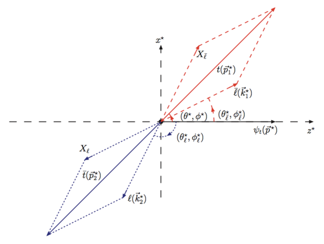
Figure 4: Definitions of the kinematical variables of top quarks and leptons in the toponium rest-frame. The $z^{\star}$ and $x^{\star}$ axes are specified by the toponium moving direction and the scattering plane in the laboratory frame, respectively.

$$\widetilde{\psi}(p;J_{\psi},\lambda_{\psi_{t}})\rightarrow t(p_{1},\sigma_{t})+\bar{t}(p_{2},\sigma_{\bar{t}})\rightarrow\bar{\ell}(k_{1})+X_{\bar{\ell}}+\ell(k_{2})+X_{\ell}\,.$$ (51)

As we have mentioned the helicity amplitudes of the toponium decay are obtained by using the spin projection of the helicity amplitudes of the $t\bar{t}$ decay. The helicity amplitudes of the $t\bar{t}$ decay can be separated into the $t$ and $\bar{t}$ decay amplitudes as

$$\mathcal{M}_{D}(\sigma_{t},\sigma_{\bar{t}}) = \langle(\ell\nu_{\bar{\ell}}\bar{b})(\bar{\ell}\nu_{\ell}b)|\mathcal{T}_{D}|t(\sigma_{t})\bar{t}(\sigma_{\bar{t}})\rangle=\mathcal{M}_{t}(\sigma_{t})\mathcal{M}_{\bar{t}}(\sigma_{\bar{t}})\,.$$ (52)

The helicity amplitudes of the $t$ and $\bar{t}$ decays have been known for long time. In the rest frame of the toponium the kinematical variables are defined as follows:

$$p_{1}^{\star\mu} = \dfrac{\sqrt{s_{\psi}}}{2}(1+\frac{m_{t}^{\star 2}-\bar{m}_{t}^{\star 2}}{s_{\psi}},\,\beta_{t}\sin\theta^{\star}\cos\phi^{\star},\,\beta_{t}\sin\theta^{\star}\sin\phi^{\star},\,\beta_{t}\cos\theta^{\star})\,,$$ (53a)

$$p_{2}^{\star\mu} = \dfrac{\sqrt{s_{\psi}}}{2}(1-\frac{m_{t}^{\star 2}-\bar{m}_{t}^{\star 2}}{s_{\psi}},\,-\beta_{t}\sin\theta^{\star}\cos\phi^{\star},\,-\beta_{t}\sin\theta^{\star}\sin\phi^{\star},\,-\beta_{t}\cos\theta^{\star})\,,$$ (53b)

$$k_{1}^{\star\mu} = E_{\bar{\ell}}(1,\,\sin\theta^{\star}_{\bar{\ell}}\cos\phi^{\star}_{\bar{\ell}},\,\sin\theta^{\star}_{\bar{\ell}}\sin\phi^{\star}_{\bar{\ell}},\,\cos\theta^{\star}_{\bar{\ell}})\,,$$ (53c)

$$k_{2}^{\star\mu} = E_{\ell}(1,\,\sin\theta^{\star}_{\ell}\cos\phi^{\star}_{\ell},\,\sin\theta^{\star}_{\ell}\sin\phi^{\star}_{\ell},\,\cos\theta^{\star}_{\ell})\,.$$ (53d)

Here and after we neglect the lepton mass. By using the Fierzt transformation, the kinematical variables of $(b\nu)/(\bar{b}\bar{\nu}_{\ell})$ can be factorized out completely. Thus the anti-lepton and lepton carry all the spin informations of $t$ and $\bar{t}$, respectively. Then the helicity amplitudes of $t$ and $\bar{t}$ decays can be written as,

$$\mathcal{M}_{t}(\sigma_{t}) = A_{t}\sqrt{E_{t}}\sqrt{E_{\bar{\ell}}}\,e^{i\sigma_{t}\phi^{\star}}$$ (54)

$$\times \bigg{(}\cos\frac{\theta^{\star}}{2}\sqrt{1+2\sigma_{t}\cos\tilde{\theta}_{\bar{\ell}}}e^{i\sigma_{t}(\phi^{\star}_{\bar{\ell}}-\phi^{\star})}+2\sigma_{t}\sin\frac{\theta^{\star}}{2}\sqrt{1-2\sigma_{t}\cos\tilde{\theta}_{\bar{\ell}}}e^{-i\sigma_{t}(\phi^{\star}_{\bar{\ell}}-\phi^{\star})}\bigg{)}\,,$$

$$\mathcal{M}_{\bar{t}}(\sigma_{\bar{t}}) = A_{\bar{t}}\sqrt{E_{t}}\sqrt{E_{\bar{\ell}}}\,e^{i\sigma_{\bar{t}}\phi^{\star}}$$ (55)

$$\times \bigg{(}\cos\frac{\theta^{\star}}{2}\sqrt{1+2\sigma_{\bar{t}}\cos\tilde{\theta}_{\ell}}e^{-i\sigma_{\bar{t}}(\phi^{\star}_{\ell}-\phi^{\star})}+2\sigma_{\bar{t}}\sin\frac{\theta^{\star}}{2}\sqrt{1-2\sigma_{\bar{t}}\cos\tilde{\theta}_{\ell}}e^{i\sigma_{t}(\phi^{\star}_{\ell}-\phi^{\star})}\bigg{)}\,,$$

where $A_{t}$ and $A_{\bar{t}}$ which are Lorentz invariant stand for the rest of the helicity amplitude.

The $t\bar{t}$ decay helicity amplitudes $\mathcal{M}_{D}(\sigma_{t},\sigma_{\bar{t}})$ can be obtained by using Eq. (52). In terms of $m$ and $\tilde{m}$, $\mathcal{M}_{D}(\sigma_{t},\sigma_{\bar{t}})$ can be written as follows:

$$\mathcal{M}_{D}(m,\tilde{m}=0) \propto \cos^{2}\frac{\theta^{\star}}{2}f_{m,-m}-\sin^{2}\frac{\theta^{\star}}{2}f_{-m,m}-\frac{1}{2}m\sin\theta^{\star}\big{(}k_{m,m}-k_{-m,-m}\big{)}\,,$$ (56a)

$$\mathcal{M}_{D}(m=0,\tilde{m}) \propto e^{i\tilde{m}\phi^{\star}}\bigg{(}\cos^{2}\frac{\theta^{\star}}{2}k_{\tilde{m},\tilde{m}}+\sin^{2}\frac{\theta^{\star}}{2}k_{-\tilde{m},-\tilde{m}}+\frac{\tilde{m}}{2}\sin\theta^{\star}\big{(}f_{\tilde{m},-\tilde{m}}+f_{-\tilde{m},\tilde{m}}\big{)}\bigg{)}\,,$$ (56b)

where the functions $f_{m,m^{\prime}}$ and $k_{m,m^{\prime}}$ are defined as follows:

$$f_{m,m^{\prime}}(\phi^{\star};\theta^{\star}_{\bar{\ell}},\phi^{\star}_{\bar{\ell}};\theta^{\star}_{\ell},\phi^{\star}_{\ell};) = g_{m,m^{\prime}}(\theta^{\star}_{\bar{\ell}},\theta^{\star}_{\ell})e^{im(\phi^{\star}_{\bar{\ell}}+\phi^{\star}_{\ell})/2}e^{im^{\prime}\phi^{\star}}\,,$$ (57)

$$k_{m,m^{\prime}}(\phi^{\star};\theta^{\star}_{\bar{\ell}},\phi^{\star}_{\bar{\ell}};\theta^{\star}_{\ell},\phi^{\star}_{\ell};) = g_{m,m^{\prime}}(\theta^{\star}_{\bar{\ell}},\theta^{\star}_{\ell})e^{im(\phi^{\star}_{\bar{\ell}}-\phi^{\star}_{\ell})/2}\,,$$ (58)

$$g_{m,m^{\prime}}(\theta^{\star}_{\bar{\ell}},\theta^{\star}_{\ell}) = \sqrt{1+m\cos\theta^{\star}_{\bar{\ell}}}\sqrt{1+m^{\prime}\cos\theta^{\star}_{\ell}}\,.$$ (59)

The projected helicity amplitudes can be obtained by using the projection operators in Eq. (30a) and Eq. (30b). As we have explained above, the production rate of the singlet toponium is highly suppressed near the threshold region. Therefore we give only the decay amplitudes for the triplet toponium. By using Eq. (22), the projected decay amplitudes for the triplet toponium are explicitely written as

$$\widetilde{\mathcal{M}}_{D}(\lambda_{\psi_{t}}=0) \propto \sqrt{2}\bigg{(}g_{1,1}(\theta^{\star}_{\bar{\ell}},\theta^{\star}_{\ell})e^{i(\phi^{\star}_{\bar{\ell}}-\phi^{\star}_{\ell})/2}-g_{-1,-1}(\theta^{\star}_{\bar{\ell}},\theta^{\star}_{\ell})e^{-i(\phi^{\star}_{\bar{\ell}}-\phi^{\star}_{\ell})/2}\bigg{)}\,,$$ (60a)

$$\widetilde{\mathcal{M}}_{D}(\lambda_{\psi_{t}}=1) \propto -\,g_{1,-1}(\theta^{\star}_{\bar{\ell}},\theta^{\star}_{\ell})e^{i(\phi^{\star}_{\bar{\ell}}+\phi^{\star}_{\ell})/2}\,,$$ (60b)

$$\widetilde{\mathcal{M}}_{D}(\lambda_{\psi_{t}}=-1) \propto ~{}~{}~{}g_{-1,1}(\theta^{\star}_{\bar{\ell}},\theta^{\star}_{\ell})e^{-i(\phi^{\star}_{\bar{\ell}}+\phi^{\star}_{\ell})/2}\,.$$ (60c)

The decay density matrix is defined as

$$\rho_{D}(\lambda_{\psi_{t}},\lambda_{\psi_{t}}^{\prime}) = \int d\Phi(b\nu;b\bar{\nu})\mathcal{M}_{D}(\lambda_{\psi_{t}})\mathcal{M}_{D}^{{\dagger}}(\lambda_{\psi_{t}}^{\prime})\,,$$ (61)

where we have integrated out the phase spaces of the bottom quarks and neutrinos. The corresponding matrix elements are

$$\rho_{D}(0,0) \propto 2\bigg{(}4\cos^{2}\frac{\theta^{\star}_{\bar{\ell}}}{2}\cos^{2}\frac{\theta^{\star}_{\ell}}{2}+4\sin^{2}\frac{\theta^{\star}_{\bar{\ell}}}{2}\sin^{2}\frac{\theta^{\star}_{\ell}}{2}-2\sin\theta^{\star}_{\bar{\ell}}\sin\theta^{\star}_{\ell}\cos(\phi^{\star}_{\bar{\ell}}-\phi^{\star}_{\ell})\bigg{)}\,,$$ (62a)

$$\rho_{D}(+,+) \propto 4\cos^{2}\frac{\theta^{\star}_{\bar{\ell}}}{2}\sin^{2}\frac{\theta^{\star}_{\ell}}{2}\,,$$ (62b)

$$\rho_{D}(-,-) \propto 4\sin^{2}\frac{\theta^{\star}_{\bar{\ell}}}{2}\cos^{2}\frac{\theta^{\star}_{\ell}}{2}\,,$$ (62c)

$$\rho_{D}(0,+) \propto 2\sqrt{2}\bigg{(}\sin\theta^{\star}_{\bar{\ell}}\sin^{2}\frac{\theta^{\star}_{\ell}}{2}e^{-i\phi^{\star}_{\bar{\ell}}}-\sin\theta^{\star}_{\ell}\cos^{2}\frac{\theta^{\star}_{\bar{\ell}}}{2}e^{-i\phi^{\star}_{\ell}}\bigg{)}\,,$$ (62d)

$$\rho_{D}(0,-) \propto 2\sqrt{2}\bigg{(}\sin\theta^{\star}_{\bar{\ell}}\cos^{2}\frac{\theta^{\star}_{\ell}}{2}e^{i\phi^{\star}_{\bar{\ell}}}-\sin\theta^{\star}_{\ell}\sin^{2}\frac{\theta^{\star}_{\bar{\ell}}}{2}e^{i\phi^{\star}_{\ell}}\bigg{)}\,,$$ (62e)

$$\rho_{D}(+,-) \propto -\sin\theta^{\star}_{\bar{\ell}}\sin\theta^{\star}_{\ell}e^{i(\phi^{\star}_{\bar{\ell}}+\phi^{\star}_{\ell})}\,.$$ (62f)

The spin correlations occur if the imaginary part of the decay density matrix is non-zero. The above results indicate that the spin correlations can appear in both the transverse-transverse and transverse-longitudinal interferences.

III.4 Total helicity amplitudes and CP-odd observables

In this subsection we discuss the interferences among the different helicity states of the triplet toponium. The CP-odd observables are obtained by studying the spin correlations due to the interferences. As we have mentioned there are two kinds of interference: transverse-transverse (TT) and longitudinal-transverse (LT) interferences, which are predicted by the total density matrix,

$$\rho = \sum_{\lambda_{V}=\pm 1}\rho(\lambda_{V})=\sum_{\lambda_{V}=\pm 1}\sum_{\lambda_{\psi_{t}}=0,\pm 1}\sum_{\lambda_{\psi_{t}}^{\prime}=0,\pm 1}\rho(\lambda_{V};\lambda_{\psi_{t}},\lambda_{\psi_{t}}^{\prime})\,$$ (63)

where for convenience we have defined an intermediate density matrix as follows:

$$\rho(\lambda_{V};\lambda_{\psi_{t}},\lambda_{\psi_{t}}^{\prime}) = \rho_{P}(\lambda_{V};\lambda_{\psi_{t}},\lambda_{\psi_{t}}^{\prime})\rho_{D}(\lambda_{\psi_{t}},\lambda_{\psi_{t}}^{\prime})\,.$$ (64)

For the TT interference we have (for convenience we use $\tilde{\xi}$ to denote the variable $\tilde{\xi}_{ht\bar{t}}$ for abbreviation),

$$\rho(\lambda_{V};\lambda_{\psi_{t}},-\lambda_{\psi_{t}}) \propto -\frac{1}{4}\sin\vartheta^{2}\sin\theta^{\star}_{\bar{\ell}}\sin\theta^{\star}_{\ell}e^{i\lambda_{\psi_{t}}(\phi^{\star}_{\bar{\ell}}+\phi^{\star}_{\ell}-2\tilde{\xi})}\,.$$ (65)

Therefore the production rate has a following non-trivial distribution with respect to the observable $\phi^{\star}_{\bar{\ell}}+\phi^{\star}_{\ell}$,

$$\frac{d\sigma}{d(\phi^{\star}_{\bar{\ell}}+\phi^{\star}_{\ell})} = \frac{1}{2\pi}\sigma_{0}\left(1-C_{TT}\cos(\phi^{\star}_{\bar{\ell}}+\phi^{\star}_{\ell}-2\tilde{\xi})\right)\,,$$ (66)

where $\sigma_{0}$ is the total cross section, and $C_{TT}$ is the coefficient for the $TT$ correlation.

For the LT interference we have

$$\rho(\lambda_{V};0,+) \propto -\sin\vartheta(1+\lambda_{V}\cos\vartheta)\bigg{(}\sin\theta^{\star}_{\bar{\ell}}\sin^{2}\frac{\theta^{\star}_{\ell}}{2}e^{-i(\phi^{\star}_{\bar{\ell}}-\tilde{\xi})}-\sin\theta^{\star}_{\ell}\cos^{2}\frac{\theta^{\star}_{\bar{\ell}}}{2}e^{-i(\phi^{\star}_{\ell}-\tilde{\xi})}\bigg{)}\,,$$ (67)

$$\rho(\lambda_{V};0,-) \propto -\sin\vartheta(1-\lambda_{V}\cos\vartheta)\bigg{(}\sin\theta^{\star}_{\bar{\ell}}\cos^{2}\frac{\theta^{\star}_{\ell}}{2}e^{i(\phi^{\star}_{\bar{\ell}}-\tilde{\xi})}-\sin\theta^{\star}_{\ell}\sin^{2}\frac{\theta^{\star}_{\bar{\ell}}}{2}e^{i(\phi^{\star}_{\ell}-\tilde{\xi})}\bigg{)}\,.$$ (68)

We can see that the azimuthal-angle distributions of lepton and anti-lepton have different $\tilde{\xi}$ dependence. The lepton momentum has a following non-trivial distribution,

$$\frac{d\sigma}{d\phi^{\star}_{\ell}} = \frac{1}{2\pi}\sigma_{0}\left(1+C_{LT}\cos(\phi^{\star}_{\ell}-\tilde{\xi})\right)\,,$$ (69)

where $C_{LT}$ is the coefficient of the $LT$ correlation. For the anti-lepton momentum, we have

$$\frac{d\sigma}{d\phi^{\star}_{\bar{\ell}}}=\frac{1}{2\pi}\sigma_{0}\left(1-C_{LT}\cos(\phi^{\star}_{\bar{\ell}}-\tilde{\xi})\right)\,.$$ (70)

We can see that the correlations are different for the lepton and anti-lepton. For the lepton, the correlation is positive, while negative for the anti-lepton. On the other hand, the sign and the size of the phase shift is the same for both the lepton and anti-lepton. These two distributions are related with each other by the CP transformation. In the case of $\tilde{\xi}=0$, i.e. CP is conserved, these two correlations are symmetric under the CP transformation $\phi^{\star}_{\bar{\ell}}\rightarrow\pi-\phi^{\star}_{\ell}$ and likewise for $\phi^{\star}_{\ell}$. However, if $\tilde{\xi}\neq 0$, the distributions are asymmetric by $\tilde{\xi}\rightarrow-\tilde{\xi}$, and therefore indicates the violation of the CP symmetry.

IV Radiative corrections near the threshold region

As we have explained in Sec. II, the virtual top or anti-top quark is hugely off-shell. According to the uncertainty principle, it can propagate only a distance $\sim 1/(\sqrt{s}-m_{t})$ which is considerably shorter than the Coulomb radius $r_{C}\sim 1/(\alpha_{s}m_{t})$ for the $t\bar{t}$ bound-state. Therefore, near threshold production can be treated by a local source $\delta^{4}(y_{t}-y_{\bar{t}})j^{\mu}(Q^{2})e^{-iQ\cdot y_{t}}$. In this approximation, the Higgs field decouples from the exact vertex function $\langle{\rm T}h(z^{\prime})\bar{t}_{i}(y_{t})t_{j}(y_{\bar{t}})V^{\mu}(z)\rangle$ by modifying the $t\bar{t}V$ vertex function which has been examined in Sec. II. The modified production vertexes are then in turn to affect the quantum numbers of the generated toponia, which have been discussed in Sec. II. Here we examine how these vertexes are affected by the QCD radiative corrections. The corrections are described by the relativistic Salpeter-Bethe (SB) equation in general SB:1951 . For a general production vertex $\Gamma^{\mu}_{C}$ (the subscript “$C$” is used to distinguish possible different Dirac matrix), the SB equation is

$$V^{\mu}_{C}(p,q) = \Gamma^{\mu}_{C}(p,q)+\int\frac{d^{4}k}{(2\pi)^{4}}\mathcal{U}_{\alpha\beta}(q-k)\gamma^{\alpha}S_{F}(p/2+k)V^{\mu}_{C}(p,k)S_{F}(-p/2+k)\gamma^{\beta}\,,$$ (71)

where $\mathcal{U}_{\alpha\beta}(q-k)$ is the QCD potential in momentum space, and $S_{F}$ is the Feynman propagator for fermions. This integral equation sums over all the contributions from the relevant ladder diagrams; see Fig. 3. Here we consider only the instantaneous Coulomb-like potential, the contributions from the transverse and rest gluons are suppressed by powers of $\beta_{t}$.

In the rest frame of $t\bar{t}$, the dominant contributions come from the region where $|\vec{k}|\ll m_{t}$, and the fermionic propagators are approximated by

$$S_{F}(p/2+k) = \frac{i(\gamma_{+}-\vec{k}\cdot\vec{\gamma}/(2m_{t}))}{E/2+k^{0}-\vec{k}^{2}/(2m_{t})+i\Gamma_{t}/2}\,,$$ (72a)

$$S_{F}(-p/2+k) = \frac{i(\gamma_{-}-\vec{k}\cdot\vec{\gamma}/(2m_{t}))}{E/2-k^{0}-\vec{k}^{2}/(2m_{t})+i\Gamma_{t}/2}\,,$$ (72b)

where $\gamma_{\pm}=(1\pm\gamma^{0})/2$ are the non-relativistic projection operators for fermion and anti-fermion. Observing that the vertex function is independent of the energy $q^{0}$, the variable $k^{0}$ can be integrated out and we get

$$V^{\mu}_{C}(E,\vec{q}) = \Gamma^{\mu}_{C}-\int\frac{d^{3}\vec{k}}{(2\pi)^{3}}U(\vec{q}-\vec{k})\gamma^{0}\bigg{(}\gamma_{+}-\frac{\vec{k}\cdot\vec{\gamma}}{2m_{t}}\bigg{)}\frac{V^{\mu}_{C}(E,\vec{k})}{E-\vec{k}^{2}/m_{t}+i\Gamma_{t}}\bigg{(}\gamma_{-}-\frac{\vec{k}\cdot\vec{\gamma}}{2m_{t}}\bigg{)}\gamma^{0}\,.$$ (73)

In our case the toponium system can be boosted by the recoil of the Higgs boson, therefore we express all the quantities in a Lorentz-invariant manner as follows:

$$E = \frac{1}{2}\sqrt{(p_{1}+p_{2})^{2}}=\frac{1}{2}\sqrt{p^{2}}\,,$$ (74a)

$$\gamma^{0} = \frac{p\!\!\!/_{1}+p\!\!\!/_{2}}{2E}=\frac{p\!\!\!/}{2E}=\frac{p\!\!\!/}{\sqrt{p^{2}}}\,,$$ (74b)

$$\gamma^{i}\gamma^{0} = \frac{1}{2}[\gamma^{\mu},\gamma^{0}]=\frac{1}{2\sqrt{p^{2}}}[\gamma^{\mu},p\!\!\!/]\equiv\widetilde{\gamma}^{\mu}\,.$$ (74c)

The integral equation can be rewritten in a covariant form as

$$V^{\mu}_{C}(E,\vec{q})=\Gamma^{\mu}_{C}+\int\frac{d^{3}\vec{k}}{(2\pi)^{3}}U(\vec{q}-\vec{k})\bigg{(}\gamma_{+}-\frac{\widetilde{k\!\!\!/}}{2m_{t}}\bigg{)}\frac{V^{\mu}_{C}(E,\vec{k})}{E-\vec{k}^{2}/m_{t}+i\Gamma_{t}}\bigg{(}\gamma_{-}-\frac{\widetilde{k\!\!\!/}}{2m_{t}}\bigg{)}\,.$$ (75)

We define the dressed non-relativistic projection operators for fermions and anti-fermions as follows:

$$\widetilde{\gamma}_{+}(\vec{q}) = \gamma_{+}-\frac{\widetilde{q\!\!\!/}}{2m_{t}}=\gamma_{+}(1-\frac{\widetilde{q\!\!\!/}}{2m_{t}})-\gamma_{-}\frac{\widetilde{q\!\!\!/}}{2m_{t}}\,,$$ (76a)

$$\widetilde{\gamma}_{-}(\vec{q}) = \gamma_{-}-\frac{\widetilde{q\!\!\!/}}{2m_{t}}=(1-\frac{\widetilde{q\!\!\!/}}{2m_{t}})\gamma_{-}-\frac{\widetilde{q\!\!\!/}}{2m_{t}}\gamma_{+}\,.$$ (76b)

The second terms in both $\widetilde{\gamma}_{+}(\vec{q})$ and $\widetilde{\gamma}_{-}(\vec{q})$ involve the small component of the Dirac spinor which are of P-wave, and therefore suppressed by an additional factor of $\beta_{t}$. Therefore in the following calculations we can neglect them. In this approximation, a useful relation can be derived as follows:

$$\gamma_{+}\widetilde{q\!\!\!/} = \widetilde{q\!\!\!/}\gamma_{-}\,.$$ (77)

Multiplying $\widetilde{\gamma}_{+}(\vec{q})$ on the left-hand side and $\widetilde{\gamma}_{-}(\vec{q})$ on the right-hand side of Eq. (75), we get

$$\widetilde{\gamma}_{+}(\vec{q})V^{\mu}_{C}(E,\vec{q})\widetilde{\gamma}_{-}(\vec{q}) \approx \widetilde{\gamma}_{+}(\vec{q})\Gamma^{\mu}_{C}\widetilde{\gamma}_{-}(\vec{q})+\int\frac{d^{3}\vec{k}}{(2\pi)^{3}}U(\vec{q}-\vec{k})\frac{\widetilde{\gamma}_{+}(\vec{k})V^{\mu}_{C}(E,\vec{k})\widetilde{\gamma}_{-}(\vec{k})}{E-\vec{k}^{2}/m_{t}+i\Gamma_{t}}\,.$$ (78)

Introducing the non-relativistic reduced vertex function

$$\widetilde{V}^{\mu}_{C}(E,\vec{q}) = \widetilde{\gamma}_{+}(\vec{q})V^{\mu}_{C}(E,\vec{q})\widetilde{\gamma}_{-}(\vec{q})\,,\quad\widetilde{\Gamma}^{\mu}_{C}=\widetilde{\gamma}_{+}(\vec{q})\Gamma^{\mu}_{C}\widetilde{\gamma}_{-}(\vec{q})\,,$$ (79)

the integral equation Eq. (78) reduces to

$$\widetilde{V}^{\mu}_{C}(E,\vec{q}) = \widetilde{\Gamma}^{\mu}_{C}(E,\vec{q})+\int\frac{d^{3}\vec{k}}{(2\pi)^{3}}U(\vec{q}-\vec{k})\frac{\widetilde{V}^{\mu}_{C}(E,\vec{k})}{E-\vec{k}^{2}/m_{t}+i\Gamma_{t}}\,.$$ (80)

This is a formal Lippmann-Schwinger (LS) equation LS:1950 . Here we study only the corrections to the production vertex up to terms linear in $\vec{q}$. Expanding the vertex $\widetilde{\Gamma}^{\mu}_{C}(E,\vec{q})$ by $\vec{q}$ we have,

$$\widetilde{\Gamma}^{\mu}_{C}(E,\vec{q}) = \mathcal{S}^{\mu}_{C}(E)-\mathcal{P}^{\mu\nu}_{C}(E)q_{\nu}\,,$$ (81)

where

$$\mathcal{S}^{\mu}_{C}(E) = \widetilde{\Gamma}^{\mu}_{C}(E,\vec{q}=0)\,,$$ (82a)

$$\mathcal{P}^{\mu\nu}_{C}(E) = \frac{\partial}{\partial q_{\nu}}\,\widetilde{\Gamma}^{\mu}_{C}(E,\vec{q})\bigg{|}_{\vec{q}=0}\,,$$ (82b)

are the S- and P-wave components, respectively. The corrected vertex function $\widetilde{V}^{\mu}_{C}(E,\vec{q})$ can be expanded in the same way, and we get

$$\widetilde{V}^{\mu}_{C}(E,\vec{q}) = \mathcal{S}^{\mu}_{C}(E)\mathcal{K}_{S}(E,\vec{q})+\vec{\mathcal{P}}^{\mu}_{C}(E)\cdot\vec{q}\;\mathcal{K}_{P}(E,\vec{q})\,.$$ (83)

The expansion coefficients satisfy following integral equations

$$\mathcal{K}_{S}(E,\vec{q}) = 1+\int\frac{d^{3}\vec{k}}{(2\pi)^{3}}U(\vec{q}-\vec{k})\frac{\mathcal{K}_{S}(E,\vec{k})}{E-\vec{k}^{2}/m_{t}+i\Gamma_{t}}\,,$$ (84a)

$$\mathcal{K}_{P}(E,\vec{q}) = 1+\int\frac{d^{3}\vec{k}}{(2\pi)^{3}}\frac{\vec{q}\cdot\vec{k}}{\vec{q}^{2}}U(\vec{q}-\vec{k})\frac{\mathcal{K}_{P}(E,\vec{k})}{E-\vec{k}^{2}/m_{t}+i\Gamma_{t}}\,.$$ (84b)

These two integral equations are related to the Green function $G(\vec{r}_{x},\vec{r}_{x})$ which satisfies the LS equation in the momentum space as follows:

$$\bigg{(}E-\frac{\vec{p}^{2}}{m_{t}}+i\Gamma_{t}\bigg{)}G(E;\vec{p},\vec{r}_{y}) = e^{i\vec{p}\cdot\vec{r}_{y}}+\int\frac{d^{3}\vec{k}}{(2\pi)^{3}}U(\vec{p}-\vec{k})G(E;\vec{k},\vec{r}_{y})\,.$$ (85)

As we have mentioned, the local interaction approximation is excellent in the production vertex, therefore the vertex functions are approximated by the condition $\vec{r}_{y}=0$. Expanding the Green function $G(E;\vec{k},\vec{r}_{y})$ by $\vec{r}_{y}$ as

$$G(E;\vec{p},\vec{r}_{y}) = G_{S}(E;\vec{p},\vec{r}_{y}=0)+(i\vec{r}_{y}\cdot\vec{p})\,G_{P}(E;\vec{p},\vec{r}_{y}=0)\,,$$ (86)

and the plane wave factor $e^{i\vec{p}\cdot\vec{r}_{y}}\approx 1+i\vec{p}\cdot\vec{r}_{y}$ we obtain the following integral equations,

$$\bigg{(}E-\frac{\vec{p}^{2}}{m_{t}}+i\Gamma_{t}\bigg{)}G_{S}(E;\vec{p}) = 1+\int\frac{d^{3}\vec{k}}{(2\pi)^{3}}U(\vec{p}-\vec{k})G_{S}(E;\vec{k})\,,$$ (87a)

$$\bigg{(}E-\frac{\vec{p}^{2}}{m_{t}}+i\Gamma_{t}\bigg{)}G_{P}(E;\vec{p}) = 1+\int\frac{d^{3}\vec{k}}{(2\pi)^{3}}\frac{\vec{p}\cdot\vec{k}}{\vec{p}^{2}}U(\vec{p}-\vec{k})G_{P}(E;\vec{k})\,.$$ (87b)

The solutions of the above equations are formally written as

$$G_{S}(E;\vec{p}) = G_{0}(E;\vec{p})+G_{0}(E;\vec{p})\int\frac{d^{3}\vec{k}}{(2\pi)^{3}}U(\vec{p}-\vec{k})G_{S}(E;\vec{k})\,.$$ (88a)

$$G_{P}(E;\vec{p}) = G_{0}(E;\vec{p})+G_{0}(E;\vec{p})\int\frac{d^{3}\vec{k}}{(2\pi)^{3}}\frac{\vec{p}\cdot\vec{k}}{\vec{p}^{2}}U(\vec{p}-\vec{k})G_{P}(E;\vec{k})\,,$$ (88b)

where $G_{0}(E;\vec{p})$ is the Green function of a free toponium,

$$G_{0}(E;\vec{p}) = \frac{1}{E-\vec{p}^{2}/m_{t}+i\Gamma_{t}}\,.$$ (89)

These Green functions are related to the correction factors $\mathcal{K}_{S}$ and $\mathcal{K}_{P}$ as follows:

$$G_{S}(E;\vec{p}) = G_{0}(E;\vec{p})\mathcal{K}_{S}(E;\vec{p}),$$ (90a)

$$G_{P}(E;\vec{p}) = G_{0}(E;\vec{p})\mathcal{K}_{P}(E;\vec{p}).$$ (90b)

In this study, we employ the method give in Ref. Jezabek:1992 to numerically solve the integral equation. Fig. 5 shows the S- and P-wave Green functions for the binding energy $E\equiv\sqrt{s_{\psi_{t}}}-2m_{t}=[-2,0,2,4]~{}{\rm GeV}$. We can see that at the ground state ($E\simeq-2~{}{\rm GeV}$), the P-wave contribution is suppressed. However, the corrections on S- and P-wave are comparable for other states. Fig. 6 shows the counter lines of the absolute values of the Green functions in the plane of the binding energy $E$ and the relative momentum $|\vec{q}|$.

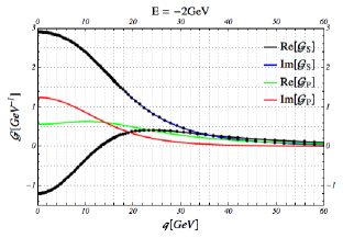
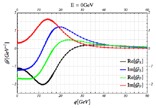
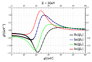
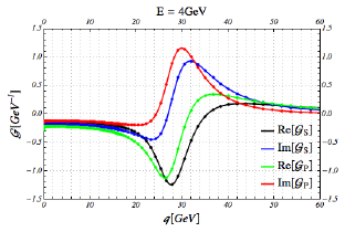
Figure 5: The Green functions as a function of $q$ for the four values of binding energy: (a) $E=-2~{}{\rm GeV}$; (b) $E=0~{}{\rm GeV}$; (c) $2~{}{\rm GeV}$; (d) $E=4~{}{\rm GeV}$.

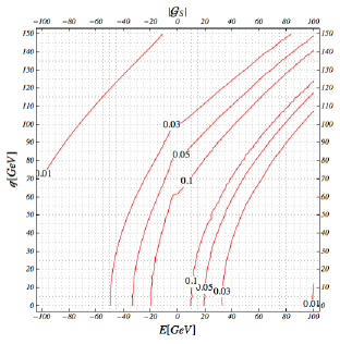
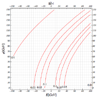
Figure 6: Contour plot of the absolute value of the Green functions for S-wave (a) and P-wave (b).

V Numerical results

Our numerical results are obtained by using MadGraph5 madgraph5 with the HC model mg5:model:hc at the tree level, and then weighted by the QCD correction factor $\mathcal{K}_{S/P}(E,\vec{q})$ at the LO. For a smooth connection to the large $M_{t\bar{t}}$ region, we follow the prescription described in Ref. Sumino:2010bv . Left and right panels in Fig. 7 show the production cross sections at $\sqrt{s}=500$ GeV with respect to the invariant mass of the $t\bar{t}$ system for the pure scalar and pure pseudo-scalar cases, respectively. We can see that the distribution of total production cross sections have a peak below the threshold energy. At this collision energy, the LO cross section is calculated to be $\sigma_{\rm LO}=0.29~{}\,{\rm fb}$ for the pure scalar case (we assume that the electron and position beams are not polarized). Note that when we include the diagram with a $hZZ$ vertex, the total cross section is enhanced by about 1.7% due to the interference with the diagrams which contain the top-Yukawa vertex. The QCD-Coulomb corrections give an enhancement factor of about $2.6$. However, it has been pointed out that the NLO corrections are important particularly in the large $t\bar{t}$ invariant mass region Farrell:2005fk ; Farrell:2006 , which gives an additional overall correction factor of about $K=0.84$ Yonamine:2011 . In total, our prediction to the total cross section is about 0.63 fb. We use this total cross section for the overall normalization. On the other hand, the NLO effects are almost uniform in the whole phase space, therefore our LO estimation can be safely used for studying the spin correlations.

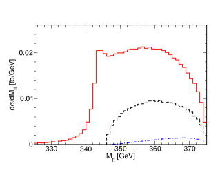
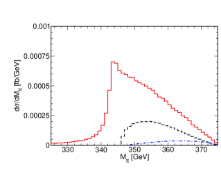
Figure 7: Production cross sections for the cases of the pure scalar case (a) and pure pseudo-scalar case (b). The black-dashed line is the cross section for the S-wave toponium at the Born level. The blue-dash-dotted line is the rest of the production cross section (which is essentially the P-wave contribution) at the Born level. The red-solid line is the total cross section after QCD-Coulomb corrections.

With the approximation of the S-wave dominance, we have calculated the azimuthal angle correlations of leptons from the decays of top and anti-top quarks. We have shown that there are three independent CP-odd observables. The first one is the sum of the azimuthal angles of leptons in the toponium rest-frame, which is due to the interference among the transverse components of the triplet toponium. The correlation function has been given in Eq. (66). Fig. 8 (a) shows the correlations for pure scalar Higgs (black-solid line) and for pure pseudo-scalar Higgs (red-dashed line). Both are symmetric under the sign reflection of $\phi_{\bar{\ell}}^{\star}+\phi_{\ell}^{\star}$, because of the CP conservation separately. However the shapes are completely opposite. In the case of scalar Higgs boson, the interference are constructive when the sum of azimuthal angles is either $\pi$ or $-\pi$. However it is constructive when the sum is $0$ for a pseudo-scalar Higgs boson. Therefore the CP violation effect is sensitive to the sign of the mixing angle $\xi_{ht\bar{t}}$. Fig. 8 (b) show three different CP-mixed cases: $\tan\xi_{ht\bar{t}}=0$ (black-solid), $\tan\xi_{ht\bar{t}}=5$ (red-dashed) and $\tan\xi_{ht\bar{t}}=-5$ (blue-dotted). Here in order to show the differences clearly we have chosen $|\tan\xi_{ht\bar{t}}|=5$ which means an effectively maximum mixing because of the kinematical suppression factor $\kappa\approx 0.2$, see Eq. (48a) and Eq. (48b). Measuring the CP violation effects from transverse-transverse interference requires the reconstructions of both lepton and anti-lepton in the topponium rest-frame. The branching ratio of top quark to leptons $(e,\mu)$ is ${\rm Br}(t\rightarrow\ell X)=19\%$. If we use the $h\rightarrow b\bar{b}$ channel to reconstruct the Higgs boson, which has a branching ratio 56.9%, there are 52 signal events with $100\%$ reconstruction efficiency for the projected integrated luminosity 4 ab^-1 at $\sqrt{s}=500~{}{\rm GeV}$ ILC:scenarios . Simple estimation on the experimental sensitivity is $\delta\tilde{\xi}_{htt}=1.34$. However, because of $\xi_{ht\bar{t}}=\tilde{\xi}_{ht\bar{t}}/\kappa$ with $\kappa\simeq 0.2$ for $\sqrt{s}=500$ GeV, the accuracy of constraining the non-zero CP-phase may be limited at the ILC with the nominal luminosity. This low sensitivity comes from 1) the low total production rate, and 2) a large kinematical suppression factor $\kappa$ in Eq. (48b).

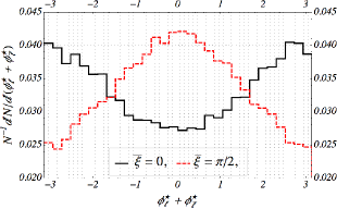
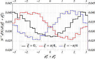
Figure 8: Azimuthal angle correlations for pure scalar and pure pseudo-scalar (a) and CP-mixed cases (b).

Apart from the interference among the transverse polarizations, there are also interferences between the longitudinally and transversely polarized toponia which result in non-trivial azimuthal angle distributions of the lepton and anti-lepton individually in the toponium rest-frame. The correlation functions are given in Eq. (69) and Eq. (70). It is constructive at the origin ($\phi_{\ell,\bar{\ell}}^{\star}=0$) for the lepton, while destructive for the anti-lepton. For the pure scalar case, this feature is shown in Fig. 9 (a). For the pure pseudo-scalar case, because only the transversely polarized toponium can be produced, there are no interference between longitudinally and transversely polarized states. Therefore the azimuthal angle distribution is flat, which is shown in Fig. 9 (b). Fig. 9 (c) and (d) show the interferences in the three cases: $\tilde{\xi}_{ht\bar{t}}=0$ (black-solid), $\tilde{\xi}_{ht\bar{t}}=\pi/4$ (red-dashed) and $\tilde{\xi}_{ht\bar{t}}=-\pi/4$ (blue-dotted) for the lepton and anti-lepton, respectively. We can see that both the lepton and anti-lepton azimuthal distributions are sensitive to the sign of the mixing angle $\tilde{\xi}_{ht\bar{t}}$. Most importantly, measuring CP violation effects through the transverse-longitudinal interferences requires only either of the lepton or anti-lepton momentum being reconstructed. For the $h\rightarrow b\bar{b}$ decay channel, there expects about 275 signal events for the projected integrated luminosity of 4 ab^-1 at $\sqrt{s}=500~{}{\rm GeV}$ ILC:scenarios (for either lepton or anti-lepton) assuming the $100\%$ reconstruction efficiency. Combining the lepton and anti-lepton channels we expect about 550 signal events in total. For this situation, the experimental sensitivity of determining $\tilde{\xi}_{ht\bar{t}}$ is estimated to be $\delta\tilde{\xi}_{ht\bar{t}}=0.4$. Taking into account the kinematical suppression factor of $\kappa\simeq 0.2$, the accuracy of determining $\xi_{ht\bar{t}}$ is estimated to be $\delta\xi_{ht\bar{t}}\simeq 1.1$ for $\xi_{ht\bar{t}}\simeq 0$.

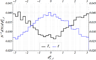
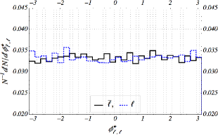
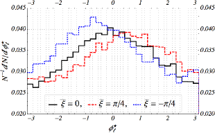
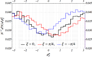
Figure 9: Azimuthal angle correlations of the lepton and anti-lepton for the cases of the pure scalar (a) and the pure pseudo-scalar Higgs boson (b). The CP-violating phase-shift is examined for $\bar{\xi}=0$, $\pi/4$ and $-\pi/4$ for the lepton (c) and the anti-lepton distributions (d).

VI Discussion and Conclusion

In summary, we have studied the CP violation effects in the toponia productions in association with a Higgs boson at the ILC with $\sqrt{s}=500~{}{\rm GeV}$. The Higgs boson can be produced by the emissions of the top or anti-top quarks via the Yukawa interaction, or through the gauge interactions between Higgs and vector bosons, $Z$ or $\gamma$. The CP violation effects can appear both in the Yukawa and gauge interactions. However observing the effects induced by the gauge interactions is difficult, because the CP-odd $hZZ$ interaction is induced at the loop level while the CP-even interaction appears at the tree level. Hence the CP asymmetry induced by the $hZZ$ coupling is suppressed by a factor of $\alpha_{W}/(4\pi)$. In addition, for the $e^{+}e^{-}$ production at $\sqrt{s}=500~{}{\rm GeV}$, the dominant contributions stem from the Higgs emissions from top quarks, but the contributions from the gauge interactions can reach only up to a few percent. Therefore, CP violation effects which emerge by the top-Yukawa couplings should be thoroughly explored.

For $\sqrt{s}=500~{}{\rm GeV}$, the produced toponia are non-relativistic, therefore the production of the P-wave toponium is negligible. The eligibility of this assumption is confirmed by the numerical calculation based on the tree-level event-generator; see Fig. 7. Furthermore, the $ht\bar{t}$ production vertex from a virtual vector boson $Z$ or $\gamma$ can be modeled by a contact vertex operator. By assuming that the spins of the top and anti-top quarks are not altered by the QCD potential, i.e. the QCD potential is spin-independent, the produced toponia spectrum are studied carefully. In this approximation, the relevant toponia are the spin-singlet ${}^{1}S_{0}$ and the spin-triplet ${}^{3}S_{1}$ states. However, the production rate of the singlet toponium is found to be highly suppressed, because it is P-wave in the toponium and Higgs boson system. This observation has been checked by using the tree-level event-generator.

Based on the careful analysis for the helicity amplitudes of the production and decay of toponia, we propose three CP-odd observables, namely the phase-shift in the azimuthal angle of the lepton and anti-lepton as well as their sum. These observables are induced by the non-trivial correlations in the longitudinal-transverse interferences in the azimuthal angle distributions of leptons, and in the transverse-transverse interference in their sum. Compared to the up-down asymmetry examined in Refs. Bhupal:2008 ; Godbole:2007 ; Godbole:2011 which requires the reconstruction of either the top- or anti-top-qaurk momenta, as well as the small contribution from the diagram which contains $hZZ$ interactions (a few percent for $\sqrt{s}\leq 1~{}{\rm TeV}$ Bhupal:2008 ), our observables do not require the reconstruction of the momentum of the top or anti-top quark individually, and are caused purely by the dominant $ht\bar{t}$ interactions. Furthermore, all the three observables have maximum asymmetries of about $32\%$, which are more than $6$ times larger than the maximum asymmetry (5%) in Refs. Godbole:2007 ; Godbole:2011 . Because the CP-odd observables for the longitudinal-transverse interferences can be reconstructed by using only the one lepton momentum, the number of signal events can be increased. The experimental sensitivities for these observables are estimated for an integrated luminosity of $L=4$ ab^-1, and found to be $\delta\xi_{ht\bar{t}}\simeq 1.1$ for $\xi_{ht\bar{t}}=0$. Since the sensitivity is limited mainly due to the statistical fluctuation, it can be improved by increasing the luminosity as projected in Ref. ILC:scenarios .

Compared to the current constraints on $\xi_{htt}$ by the LHC measurement, which has set $\xi_{htt}<0.6\pi$ Kobakhidze:2014gqa , and further improvements by future LHC measurements, the sensitivities of our observables may be relatively low, $\delta\xi_{ht\bar{t}}\simeq 1.1$ for $\xi_{ht\bar{t}}=0$. However, our observables can be used to directly measure the CP phase, rather than to measure the overall rates. Particularly, our observables $\phi_{\ell}$ and $\phi_{\bar{\ell}}$ require either top or anti-top decaying to leptons, and therefore the efficiency would be enhanced dramatically.

VII Appendix

VII.1 Spinor wave functions in the Dirac representation

For completeness we give our conventions for the spinor wave functions in the Dirac representation. In the Dirac representation, Dirac matrixes are given as follows:

$$\gamma^{0}_{D} = \left(\begin{array}[]{cc}1&0\\ 0&-1\end{array}\right)\,,\;\;\;\vec{\gamma}_{D}=\left(\begin{array}[]{cc}0&\vec{\sigma}\\ -\vec{\sigma}&0\end{array}\right)\,.$$ (95)

The free solutions of the Dirac equation in the Dirac representation are

$$u_{D}(\vec{p}_{1},s) = \left(\begin{array}[]{c}\xi_{s}\\[8.53581pt] \dfrac{\vec{\sigma}\cdot\vec{p}_{1}}{E+m}\xi_{s}\end{array}\right)\,,\;\;\;v_{D}(\vec{p}_{2},r)=\left(\begin{array}[]{c}r\dfrac{\vec{\sigma}\cdot\vec{p}_{2}}{E+m}\eta_{-r}\\[8.53581pt] r\eta_{-r}\end{array}\right)\,,$$ (100)

where $\xi_{s}$ and $\eta_{r}$ are eigenstates of the helicity operators $\vec{\sigma}\cdot\vec{p}_{1}/|\vec{p}_{1}|$ and $\vec{\sigma}\cdot\vec{p}_{2}/|\vec{p}_{2}|$, respectively. For completeness we also give the helicity eigenstates as follows:

$$\xi_{+} = \left(\begin{array}[]{c}\cos(\theta/2)\\ e^{i\phi}\sin(\theta/2)\end{array}\right)\,,\;\;\;\xi_{-}=\left(\begin{array}[]{c}-e^{-i\phi}\sin(\theta/2)\\ \cos(\theta/2)\end{array}\right)\,.$$ (105)

The spinor wave functions and the Dirac gamma matrices in the Dirac representation are related to the ones in the chiral representation by the following unitary transformation:

$$\psi_{D} = U_{D}\psi U_{D}^{-1}\,,\;\;\;\gamma^{\mu}_{D}=U_{D}\gamma_{C}^{\mu}U_{D}^{-1}\,,\;\;\;U_{D}=\frac{1}{\sqrt[]{2}}\left(\begin{array}[]{cc}1&1\\ -1&1\end{array}\right)\,.$$ (108)

VII.2 Vector wave functions and Wigner-D functions

The helicity wave functions polarized along the direction $\vec{n}=(\sin\theta\cos\phi,\,\sin\theta\sin\phi,\,\cos\theta)$ for vector particles in the rest frame are defined as follows:

$$\epsilon(\vec{n},\lambda=\pm 1) = \dfrac{1}{\sqrt{2}}(0,\,-\lambda\cos\theta\cos\phi+i\sin\phi,\,-\lambda\cos\theta\sin\phi-i\cos\phi,\,\lambda\sin\theta)\,,$$ (109)

$$\epsilon(\vec{n},\lambda=0) = (0,\,\sin\theta\cos\phi,\,\sin\theta\sin\phi,\,\cos\theta)$$ (110)

The Wigner-D function for spin-1 particle is defined as follows:

$$\vec{\epsilon}(\vec{n},\lambda^{\prime}) = \sum_{\lambda=0,\pm 1}D^{J=1}_{\lambda\lambda^{\prime}}(\theta,\phi)\,\vec{\epsilon}(\vec{0},\lambda)$$ (111)

and it’s inverse

$$\vec{\epsilon}(\vec{0},\lambda) = \sum_{\lambda^{\prime\prime}=0,\pm 1}\widetilde{D}^{J=1}_{\lambda^{\prime\prime}\lambda}(\theta,\phi)\,\vec{\epsilon}(\vec{n},\lambda^{\prime\prime})$$ (112)

and following relation holds

$$\widetilde{D}^{J=1}_{\lambda^{\prime}\lambda}(\theta,\phi) = (D^{J=1}_{\lambda\lambda^{\prime}}(\theta,\phi))^{\ast}$$ (113)

Based on these definitions we also have

$$\vec{\epsilon}^{\;\ast}(\vec{n},\lambda^{\prime})\cdot\vec{\epsilon}(\vec{0},\lambda) = \widetilde{D}^{J=1}_{\lambda^{\prime}\lambda}(\theta,\phi)$$ (114)

$$\vec{\epsilon}^{\;\ast}(\vec{0},\lambda)\cdot\vec{\epsilon}(\vec{n},\lambda^{\prime}) = D^{J=1}_{\lambda\lambda^{\prime}}(\theta,\phi)$$ (115)

References

- (1) G. Aad et al. . (ATLAS Collaboration), Observation of a new particle in the search for the Standard Model Higgs boson with the ATLAS detector at the LHC, Phys. Lett. B 716, 1 (2012).
- (2) S. Chatrchyan et al. (CMS Collaboration), Observation of a new boson at a mass of 125 GeV with the CMS experiment at the LHC, Phys. Lett. B 716, 30 (2012).
- (3) G. Aad et al. . (ATLAS Collaboration), Evidence for the spin-0 nature of the Higgs boson using ATLAS data, Phys. Lett. B 726, 120 (2013).
- (4) S. Chatrchyan et al. (CMS Collaboration), Study of the Mass and Spin-Parity of the Higgs Boson Candidate via Its Decays to Boson Pairs, Phys. Rev. Lett. 110, 081803 (2013); Erratum Phys. Rev. Lett. 110, 189901 (2013).
- (5) S. Chatrchyan et al. (CMS Collaboration), Measurement of the properties of a Higgs boson in the four-lepton final state, Phys. Rev. D 89, 092007 (2014).
- (6) A. Kobakhidze, L. Wu and J. Yue, “Anomalous Top-Higgs Couplings and Top Polarisation in Single Top and Higgs Associated Production at the LHC”, JHEP, 10, 100(2014).
- (7) J. Ellis, T. You, “Updated global analysis of Higgs couplings”, JHEP, 06, 103(2013).
- (8) H. Abe, T. Kobayashi, H. Ohki, K. Sumita, Y. Tatsuta, “Flavor landscape of 10D SYM theory with magnetized extra dimensions”, JHEP, 04, 007(2014).
- (9) K. Nishiwaki, S. Niyogi, A. Shivaji, “ anomalous coupling in double Higgs production”, JHEP, 04, 011(2014).
- (10) S. Klevtsov, S. Zelditch, “Stability and integration over Bergman metrics”, JHEP, 07, 100(2014).
- (11) J. Brod, U. Haisch, and J. Zupan, Constraints on CP-violating Higgs couplings to the third generation, JHEP 1311, 180 (2013).
- (12) J. Shu and Y. Zhang, Impact of a CP-Violating Higgs Sector: From LHC to Baryogenesis, Phys. Rev. Lett. 111, 091801 (2013).
- (13) M. J. Dolan, P. Harris, M. Jankowiak, M. Spannowsky, Constraining CP-violating Higgs Sectors at the LHC using gluon fusion, Phys. Rev. D 90, 073008 (2014).
- (14) S. Bolognesi, Y. Gao, A. V. Gritsan, K. Melnikov, M. Schulze, et al. , On the spin and parity of a single-produced resonance at the LHC, Phys. Rev. D 86, 095031 (2012).
- (15) Y. Chen, A. Falkowski, I. Low, R. V.-Morales, New Observables for CP Violation in Higgs Decays, Phys. Rev. D 90, 113006 (2014).
- (16) Y. Chen, R. Harnik, R. V.-Morales, Probing the Higgs Couplings to Photons in at the LHC, Phys. Rev. Lett. 113, 191801 (2014).
- (17) F. Bishara, Y. Grossman, R. Harnik, D. J. Robinson, J. Shu and J. Zupan, Probing CP Violation in with Converted Photons, J. High Energy Phys. 04, 084 (2014).
- (18) A. Y. Korchin, V. A. Kovalchuk, Polarization effects in the Higgs boson decay to gamma Z and test of CP and CPT symmetries, Phys. Rev. D 88, 036009 (2013).
- (19) W. Bernreuther, P. Gonzalez, M. Wiebusch, Pseudoscalar Higgs Bosons at the LHC: Production and Decays into Electroweak Gauge Bosons Revisited, Eur. Phys. J. C 69, 31 (2010).
- (20) T. Plehn, D. Rainwater, and D. Zeppenfeld, Determining the Structure of Higgs Couplings at the CERN Large Hadron Collider, Phys. Rev. Lett. 88, 051801 (2002).
- (21) J. R. DellユAquila and C. A. Nelson, Use of the or decay mode to distinguish an intermediate mass Higgs boson from a technipion, Nucl. Phys. B 320, 86 (1989).
- (22) J. R. DellユAquila and C. A. Nelson, CP determination for new spin zero mesons by the decay mode, Nucl. Phys. B 320, 61 (1989).
- (23) R. Harnik, A. Martin, T. Okui, R. Primulando, and F. Yu, Measuring CP Violation in at Colliders, Phys. Rev. D 88, 076009 (2013).
- (24) G. Bower, T. Pierzchala, Z. Was, and M. Worek, Measuring the Higgs boson’s parity using , Phys. Lett. B 543, 227 (2002).
- (25) K. Desch, Z. Was, and M. Worek, Measuring the Higgs boson parity at a Linear Collider using the tau impact parameter and decay, Eur. Phys. J. C 29, 491 (2003).
- (26) S. Berge, W. Bernreuther, and J. Ziethe, Determining the CP Parity of Higgs Bosons via Their Decay Channels at the Large Hadron Collider, Phys. Rev. Lett. 100, 171605 (2008).
- (27) S. Berge and W. Bernreuther, Determining the CP parity of Higgs bosons at the LHC in the to 1-prong decay channels, Phys. Lett. B 671, 470 (2009).
- (28) S. Berge, W. Bernreuther, B. Niepelt, and H. Spiesberger, How to pin down the CP quantum numbers of a Higgs boson in its tau decays at the LHC, Phys. Rev. D 84, 116003 (2011).
- (29) S. Berge, W. Bernreuther, and H. Spiesberger, Higgs CP properties using the tau decay modes at the ILC, Phys. Lett. B 727, 488 (2013).
- (30) K. Hagiwara, J. Nakamura, Study on the azimuthal angle correlation between two jets in the top quark pair production, arXiv:1501.00794.
- (31) J. Brod, U. Haisch and J. Zupan, Constraints on CP-violating Higgs couplings to the third generation, JHEP 1311, 180 (2013).
- (32) K. Nishiwaki, S. Niyogi and A. Shivaji, Anomalous Coupling in Double Higgs Production, JHEP 1404, 011 (2014).
- (33) J. Ellis, D. S. Hwang, K. Sakurai and M. Takeuchi, Disentangling Higgs-Top Couplings in Associated Production, JHEP 1404, 004 (2014).
- (34) F. Demartin, F. Maltoni, K. Mawatari, B. Page and M. Zaro, Higgs characterisation at NLO in QCD: CP properties of the top-quark Yukawa interaction, Eur. Phys. J. C 74, no. 9, 3065 (2014).
- (35) X. G. He, G. N. Li and Y. J. Zheng, Probing Higgs boson Properties with at the LHC and the 100 TeV collider, Int. J. Mod. Phys. A 30, no. 25, 1550156 (2015).
- (36) F. Boudjema, R. M. Godbole, D. Guadagnoli and K. A. Mohan, Lab-frame observables for probing the top-Higgs interaction, Phys. Rev. D 92, no. 1, 015019 (2015).
- (37) K. Kołodziej and A. Słapik, Probing the top-Higgs coupling through the secondary lepton distributions in the associated production of the top-quark pair and Higgs boson at the LHC, Eur. Phys. J. C 75, no. 10, 475 (2015).
- (38) M. Casolino, T. Farooque, A. Juste, T. Liu and M. Spannowsky, Probing a light CP-odd scalar in di-top-associated production at the LHC, Eur. Phys. J. C 75, 498 (2015).
- (39) M. R. Buckley and D, Goncalves, Boosting the Direct CP Measurement of the Higgs-Top Coupling, arXiv:1507.07926.
- (40) P. S. Bhupal Dev, A. Djouadi, R. M. Godbole, M. M. Mühlleitner, and S. D. Rindani, Determining the CP Properties of the Higgs Boson, Phys. Rev. Lett. 100, 051801 (2008).
- (41) R. M. Godbole, P.S. Bhupal Dev, A. Djouadi, M. M. Mühlleitner, S.D. Rindani, Probing CP properties of the Higgs Boson via , arXiv:0710.2669, ECONF C0705302:TOP08,2007.
- (42) R. M. Godbole, C. Hangst, M. Mühlleitner, S. D. Rindani, P. Sharma, Model-independent analysis of Higgs spin and CP properties in the process , Eur. Phys. J. C 71, 1681 (2011).
- (43) B. Ananthanarayan, S. K. Garg, J. Lahiri and P. Poulose, Probing the indefinite CP nature of the Higgs boson through decay distributions in the process , Phys. Rev. D 87, no. 11, 114002 (2013).
- (44) B. Ananthanarayan, S. K. Garg, C. S. Kim, J. Lahiri and P. Poulose, Top Yukawa coupling measurement with indefinite CP Higgs in , Phys. Rev. D 90, no. 1, 014016 (2014).
- (45) T. Barklow, J. Brau, K. Fujii, J. Gao, J. List, N. Walker, K. Yokoya, ILC Operating Scenarios, arXiv:1506.07830.
- (46) H. Baer et al., The International Linear Collider Technical Design Report - Volume 2: Physics, arXiv:1306.6352 [hep-ph].
- (47) K. Fujii et al., Physics Case for the International Linear Collider, arXiv:1506.05992 [hep-ex].
- (48) E. E. Salpeter and H. A. Bethe, A Relativistic Equation for Bound-State Problems, Phys. Rev. 84, 1232 (1951).
- (49) B. A. Lippmann and J. Schwinger, Variational Principles for Scattering Processes, Phys. Rev. 79, 469 (1950).
- (50) M. Jeżabek, J. H. Kühn and T. Teubner, Momentum distributions in production and decay near threshold, Z. Phy. C 56, 653 (1992).
- (51) J. Alwall, M. Herquet, F. Maltoni, O. Mattelaer, and T. Stelzer, MadGraph 5 : Going Beyond, J. High Energy Phys. 06, 128 (2011).
- (52) P. Artoisenet, P. Artoisenet, P. de Aquino, F. Demartin, R. Frederix et al. , A framework for Higgs characterisation, J. High Energy Phys. 11, 043 (2013).
- (53) Y. Sumino and H. Yokoya, Bound-state effects on kinematical distributions of top quarks at hadron colliders, JHEP 1009, 034(2010).
- (54) C. Farrell and A. H. Hoang, The Large Higgs energy region in Higgs associated top pair production at the linear collider, Phys. Rev. D 72, 014007 (2005).
- (55) C. Farrell and A. H. Hoang, Next-to-leading-logarithmic QCD corrections to the cross section at , Phys. Rev. D 74, 014008 (2006).
- (56) R. Yonamine, K. Ikematsu, T. Tanabe, K. Fujii, Y. Kiyo, Y. Sumino, and H. Yokoya, Measuring the top Yukawa coupling at the ILC at , Phys. Rev. D 84, 014033 (2011).