A non-linear subdiffusion model for a cell-cell adhesion in chemotaxis

Akram Al-Sabbagh^a,b

^aSchool of Mathematics, The university of Manchester, Manchester, Oxford Road, M13 9PL, UK

^bDept. of Mathematics and Computer Applications, Al-Nahrrain University, 64055 Baghdad, Iraq

Abstract. The purpose of this work is to propose a non-Markovian and nonlinear model of subdiffusive transport that involves adhesion affects the cells escape rates form position $x$, with chemotaxis. This leads the escape rates to be dependent on the particles density at the neighbours as well as the chemotactic gradient. We systematically derive subdiffusive fractional master equation, then we consider the diffusive limit of the fractional master equation. We finally solve the resulted fractional subdiffusive master equation stationery and analyse the role of adhesion in the resulted stationary density.

1. Introduction

In recent years, a stochastic model has become one important tool to deal with the aspect of cell (or organism) migration and adhesion [1, 2, 3, 4, 5, 6, 7]. Cell-cell adhesion is a fundamental phenomenon in regard to the subject of cells binding to each other using their surface proteins that are known as cell adhesion molecules [2]. Cell migration and adhesion play a key role in many biological phenomena, such as biomolecules [8], granular media [9], cell development [10] and tissue formation, stability and breakdown [2] as cells transport to their targets and, by adhesion, they aggregate to from different types of tissues that could be controlled by varying the level of expression of cell adhesion molecules [11].

In general, cell migration can be modelled using two techniques [12], the first is the stochastic (individual–based) model that involves randomness, which is how biological systems behave prevalently, while the other form is deterministic (population-based); this model involves systems of partial differential equations which make it easier to deal with and also more useful for some biological systems [7]. However, those two forms can be married by understanding the mechanism of cell adhesion that uses the individual-level properties that rules many biological behaviours [3].

Cell adhesion models, on the other hand, can be divided into three forms; the discrete approach, which has been widely used to describe many cell migration applications, such as the migration of glioma cell [13, 14], cancer cell invasion [15, 4, 14], wound healing [3] and many other [13, 4, 16, 17, 6]. The second form of cell adhesion modelling is the continuum model, but there are not many attempts on that subject in the literature [1, 2, 3]; some of them were derived by taking the continuous limit of the discrete model. The last type of adhesion modelling is the hybrid model in which both the discrete and the continuous model is combined, and that is even less common [18, 5, 7].

The subject of cell movement related to the mean field density has been reported by many authors [13, 4, 16, 17]. It shows the physical behaviour of non-linear diffusive discrete models. However there are few recent attempts in order to derive a CTRW model with nonlinear reaction [19, 20]. Since the CTRW model has become one popular tool to deal with anomalous diffusion, Fedotov and his collaborators have derived CTRW models for anomalous diffusion process with density dependence jumping rates [21, 22, 23].

The aim in this work is to complete our work in [23] by taking into account of nonlinear dependence on adhesion with anomalous subdiffusion transition in chemotaxis. Therefore, we attempt to derive a non-Markovian random walk model with subdiffusive transport depending on the mean field density together with adhesive effects. In [23], we derived the generalised non-linear fractional equation in a diffusion limit as

$$\frac{\partial\rho}{\partial t} =\frac{\partial{}}{\partial x}\left[\frac{l^{2}}{g(x)}\frac{dS(x)}{dx}e^{-\Phi(x,t)}\mathcal{D}_{t}^{1-\nu(x)}\rho(x,t)e^{\Phi(x,t)}-l^{2}\kappa\frac{\partial\rho}{\partial x}\alpha(\rho)\right]$$

$$+\frac{\partial^{2}{}}{\partial x^{2}}\left[\frac{l^{2}}{2g(x)}e^{-\Phi(x,t)}\mathcal{D}_{t}^{1-\nu(x)}\rho(x,t)e^{\Phi(x,t)}+\alpha(\rho)\rho(x,t)\right],$$ (1.1)

Where doth diffusion and transport are regarded to chemotaxis and the mean field density. In this work, however, we assume the adhesion affects the jumping rate to the right and left $\lambda$ and $\mu$. Section 2. presents the derivation of a non-Markovian nonlinear model with density dependence jumping rate, whereas in section 4. we derive the generalized master equation in diffusion limit, and in section 5. we describe the aggregation phenomena in anomalous subdiffusion.

2. Non-Markovian nonlinear model

In this section we use the same technique we used in [23] in order to derive the generalized non-linear master equation. We assume a particle moves randomly on a one-dimensional lattice with waiting $T_{x}$ time between two jumps. The jump direction would be detected by the minimum of two independent random times $T_{x}^{\lambda}$ (waiting time preceding jump to the right) and $T_{x}^{\mu}$ (waiting time preceding jump to the left). Therefore, the particle jumps to the right if $T_{x}^{\lambda}<T_{x}^{\mu}$ and jumps to the left otherwise. Then the particle’s actual waiting time is

$$T_{x}=\min\{T_{x}^{\lambda},T_{x}^{\mu}\}.$$ (2.1)

Where $T_{x}^{\lambda}$ and $T_{x}^{\mu}$ are distributed as the waiting time PDFs $\psi_{\lambda}(x,\tau)$ and $\psi_{\mu}(x,\tau)$ respectively, where $\tau$ is the particle’s residence time at position $x$. The waiting time PDFs $\psi_{\lambda}(x,\tau)$ and $\psi_{\mu}(x,\tau)$ are defined as the limit

$$\psi_{\lambda}(x,\tau)=\lim_{\Delta\tau\rightarrow 0}\frac{\Pr\{\tau<T_{x}^{\lambda}<\tau+\Delta t\}}{\Delta t},\ \ \ \ \ \psi_{\mu}(x,\tau)=\lim_{\Delta\tau\rightarrow 0}\frac{\Pr\{\tau<T_{x}^{\mu}<\tau+\Delta t\}}{\Delta t}.$$ (2.2)

Accordingly, the survival function PDFs of jumping to the right and left are defined relative to the waiting time PDFs as

$$\Psi_{\lambda}(x,\tau)=\int_{\tau}^{\infty}\psi_{\lambda}(x,s)ds,\ \ \ \ \ \Psi_{\mu}(x,\tau)=\int_{\tau}^{\infty}\psi_{\mu}(x,s)ds.$$ (2.3)

At this stage, we will introduce the modified escape rates of particles to the right $\lambda_{\alpha}$ and to the left $\mu_{\alpha}$, where these escape rates are now depend on the density of particles at the neighbour as well as the particle position $x$ and its residence time $\tau$. They are defined as

$$\lambda_{\alpha}=\lambda(x,\tau)+\alpha_{\lambda}(\rho(x-l,t)),\ \ \ \ \ \mu_{\alpha}=\mu(x,\tau)+\alpha_{\mu}(\rho(x+l,t)).$$ (2.4)

Here, $\lambda(x,\tau)$ and $\mu(x,\tau)$ represent the linear escape rates with no mean field density dependence and are defined as

$$\lambda(x,\tau)=\lim_{\Delta\tau\rightarrow 0}\frac{\Pr\{T_{x}^{\lambda}<\tau+\Delta t|T_{x}^{\lambda}>\tau\}}{\Delta t},\ \ \ \ \ \mu(x,\tau)=\lim_{\Delta\tau\rightarrow 0}\frac{\Pr\{T_{x}^{\mu}<\tau+\Delta t|T_{x}^{\mu}>\tau\}}{\Delta t},$$ (2.5)

And $\alpha_{\lambda}(\rho(x-l,t))$ and $\alpha_{\mu}(\rho(x+l,t))$ are the addition nonlinear escape rates with adhesion effects. The nonlinear term in escape rates are independent of the anomalous trapping with probability of escaping equal to $\alpha(\rho)\Delta t$ in a time interval of $\Delta t$, and

$$\alpha(\rho(x,t))=\alpha_{\lambda}(\rho(x-l,t))+\alpha_{\mu}(\rho(x+l,t)).$$ (2.6)

This flexible form of escape rates leads us to generalize several nonlinear effects, for instance by the following choice of escape rates,

$$\lambda_{\alpha}=\lambda(x,\tau)+\alpha_{\lambda}(\rho(x+l,t)),\ \ \ \ \ \mu_{\alpha}=\mu(x,\tau)+\alpha_{\mu}(\rho(x-l,t)),$$ (2.7)

the volume filling effects can be obtained, where particles that have a non-zero volume prevent other particles from diffusing through the occupied area [24, 25]. Also, those escape rates could lead to the model of the local gradient of density [25] by choosing [23]

$$\lambda_{\alpha}=\lambda(x,\tau)+\kappa(\alpha_{\lambda}(\rho(x+l,t))-\alpha_{\lambda}(\rho(x,t))),\ \ \ \ \ \mu_{\alpha}=\mu(x,\tau)+\kappa(\alpha_{\mu}(\rho(x,t))-\alpha_{\mu}(\rho(x-l,t))).$$ (2.8)

The escape rates $\lambda$ and $\mu$ could also be written in terms of both the waiting time PDF and the survival function, by the use of Bayes’ theorem, as

$$\lambda(x,\tau)=\frac{\psi_{\lambda}(x,\tau)}{\Psi(x,\tau)},\ \ \ \ \ \mu(x,\tau)=\frac{\psi_{\mu}(x,\tau)}{\Psi(x,\tau)},$$ (2.9)

Where $\Psi(x,\tau)$ represents the total survival PDF, which is basically the product of the two survival functions $\Psi_{\lambda}$ and $\Psi_{\mu}$, and is also defined as

$$\Psi(x,\tau)=e^{-\int_{0}^{\tau}(\lambda(x,s)+\mu(x,s))ds}.$$ (2.10)

The total waiting time PDF $\psi(x,\tau)$, in addition, is defined to be the summation of the waiting time PDF of jumping to the right $\psi_{\lambda}(x,\tau)$ and to the left $\psi_{\mu}(x,\tau)$, that are defined as

$$\psi_{\lambda}(x,\tau)=\frac{-\partial\Psi_{\mu}(x,\tau)}{\partial\tau}\Psi_{\lambda}(x,\tau),\ \ \ \ \ \psi_{\mu}(x,\tau)=\frac{-\partial\Psi_{\lambda}(x,\tau)}{\partial\tau}\Psi_{\mu}(x,\tau).$$ (2.11)

In order to derive the generalized master equation for the non-Markovian model, we follow the procedure of adding an auxiliary variable $\tau$ to generate a structured density $\xi(x,t,\tau)$ that represent the particle density at position $x$ at time $t$ being trapped for time $\tau$ [19, 26, 27, 23]. This structured density should obey the balance equation

$$\frac{\partial\xi}{\partial t}+\frac{\partial\xi}{\partial\tau} =-(\lambda(x,\tau)+\alpha_{\lambda}(\rho(x-l,t))\xi(x,t,\tau)$$

$$-(\mu(x,\tau)+\alpha_{\mu}(\rho(x+l,t))\xi(x,t,\tau).$$ (2.12)

The target now is to derive the general form of the unstructured density $\rho(x,t)$, where

$$\rho(x,t)=\int_{0}^{t}\xi(x,t,\tau)d\tau.$$ (2.13)

This approach has been found to be one useful technique to deal with non-Markovian random walk [28, 29, 30, 26, 27], especially for the nonlinear generalizations [21, 31, 32, 22, 23]. The balance equation (2.) needs to satisfy the initial condition for $t=0$ that is given by

$$\xi(x,0,\tau)=\rho_{0}(x)\delta(\tau),$$ (2.14)

Where $\rho_{0}(x)$ is the initial density of particles and $\delta$ is the Dirac delta function. Also, the boundary condition where the residence time $\tau=0$ is given by

$$\xi(x,t,0) =\int_{0}^{t}[\lambda(x-l,\tau)+\alpha_{\lambda}(\rho(x-2l,t))]\xi(x-l,t,\tau)d\tau$$

$$+\int_{0}^{t}[\mu(x+l,\tau)+\alpha_{\mu}(\rho(x+2l,t))]\xi(x+l,t,\tau)d\tau.$$ (2.15)

Denote the integral arrival rate as $j(x,t)$, which represents the rate of particles that arrive to position $x$ at exactly time $t$. This rate is equivalent to the boundary condition above (2.), that is

$$j(x,t)=\xi(x,t,0).$$ (2.16)

We introduce the integral escape rates to the right $i_{\lambda}$ and to the left $i_{\mu}$ as

$$i_{\lambda}(x,t) =\int_{0}^{t}\lambda_{\alpha}\xi(x,t,\tau)d\tau,$$

$$i_{\mu}(x,t) =\int_{0}^{t}\mu_{\alpha}\xi(x,t,\tau)d\tau.$$ (2.17)

Then the boundary condition (2.) can now be presented as

$$j(x,t)=i_{\lambda}(x-l,t)+i_{\mu}(x+l,t).$$ (2.18)

In order to get the final form for the generalised master equation for the unstructured density, we first solve the balance equation (2.) using the method of characteristics and get

$$\xi(x,t,\tau)=\xi(x,t-\tau,0)e^{-\int_{0}^{\tau}(\lambda(x,s)+\mu(x,s))ds}e^{-\int_{t-\tau}^{t}\alpha(\rho)ds},$$ (2.19)

or in other words,

$$\xi(x,t,\tau)=j(x,t-\tau)\Psi(x,\tau)e^{-\int_{t-\tau}^{t}\alpha(\rho)ds},$$ (2.20)

where $\alpha(\rho)=\alpha_{\lambda}(\rho(x-l,t))+\alpha_{\mu}(\rho(x+l,t))$. Inserting the characteristics solution (2.20) into (2.13), and by the use of the initial condition (2.14), one can get

$$\rho(x,t)=\int_{0}^{t}\Psi(x,\tau)j(x,t-\tau)e^{-\int_{t-\tau}^{t}\alpha(\rho)ds}d\tau+\rho_{0}(x)\Psi(x,t)e^{-\int_{0}^{t}\alpha(\rho)ds}.$$ (2.21)

Hence, the integral escape rates to the right and left in equation (2.) can be represented using the solution of (2.20) in the form

$$i_{\lambda}(x,t) =\int_{0}^{t}\psi_{\lambda}(x,\tau)j(x,t-\tau)e^{-\int_{t-\tau}^{t}\alpha(\rho)ds}d\tau$$

$$+\rho_{0}(x)\psi_{\lambda}(x,t)e^{-\int_{0}^{t}\alpha(\rho)ds}+\alpha_{\lambda}(\rho(x-l,t))\rho(x,t),$$

$$i_{\mu}(x,t) =\int_{0}^{t}\psi_{\mu}(x,\tau)j(x,t-\tau)e^{-\int_{t-\tau}^{t}\alpha(\rho)ds}d\tau$$

$$+\rho_{0}(x)\psi_{\mu}(x,t)e^{-\int_{0}^{t}\alpha(\rho)ds}+\alpha_{\mu}(\rho(x+l,t))\rho(x,t).$$ (2.22)

Finally, to eliminate the expression of the arrival rate $j(x,t)$ from the above form, we apply the Laplace transform on (2.) and then invert the transport to obtain

$$i_{\lambda}(x,t) =\int_{0}^{t}K_{\lambda}(x,t-\tau)\rho(x,\tau)e^{-\int_{0}^{t}\alpha(\rho)ds}d\tau+\alpha_{\lambda}(\rho(x-l,t))\rho(x,t),$$

$$i_{\mu}(x,t) =\int_{0}^{t}K_{\mu}(x,t-\tau)\rho(x,\tau)e^{-\int_{0}^{t}\alpha(\rho)ds}d\tau+\alpha_{\mu}(\rho(x+l,t))\rho(x,t),$$ (2.23)

where $K_{\lambda}$ and $K_{\mu}$ are the memory kernels that are defined in Laplace space as

$$\hat{K}_{\lambda}(x,s)=\frac{\hat{\psi}_{\lambda}(x,s)}{\hat{\Psi}(x,s)},\ \ \ \ \ \hat{K}_{\mu}(x,s)=\frac{\hat{\psi}_{\mu}(x,s)}{\hat{\Psi}(x,s)}.$$ (2.24)

In order to get the final approach of the master equation for the unstructured density, we differentiate (2.13) with respect to $t$, and use the balance equation of the structured density (2.) to get

$$\frac{\partial\rho}{\partial t}=j(x,t)-i_{\lambda}(x,t)-i_{\mu}(x,t)$$

or

$$\frac{\partial\rho}{\partial t}=i_{\lambda}(x-l,t)+i_{\mu}(x+l,t)-i_{\lambda}(x,t)-i_{\mu}(x,t).$$ (2.25)

This equation is described as the balance of particles that arrive to and leave from the state $x$ at time $t$. Therefore, the final expression of the generalised master equation for the unstructured density can be formulated as

$$\frac{\partial\rho}{\partial t} =\int_{0}^{t}K_{\lambda}(x-l,t-\tau)\rho(x-l,\tau)e^{-\int_{0}^{t}\alpha(\rho(x-l,t))ds}d\tau+\alpha_{\lambda}(\rho(x-2l,t))\rho(x-l,t)$$

$$+\int_{0}^{t}K_{\mu}(x+l,t-\tau)\rho(x+l,\tau)e^{-\int_{0}^{t}\alpha(\rho(x+l,t))ds}d\tau+\alpha_{\mu}(\rho(x+2l,t))\rho(x+l,t)$$

$$-\int_{0}^{t}K(x,t-\tau)\rho(x,\tau)e^{-\int_{0}^{t}\alpha(\rho)ds}d\tau-\alpha(\rho)\rho(x,t),$$ (2.26)

where $K(x,t)=K_{\lambda}(x,t)+K_{\mu}(x,t)$ is the combined memory kernel and $\alpha(\rho)=\alpha_{\lambda}(\rho(x-l,t))+\alpha_{\mu}(\rho(x+l,t))$.

3. Anomalous subdiffusion model

In this section we deal with a special case of the generalised master equation (2.) and derive the fractional master equation for our model. Assuming that the escape rates are inversely proportional to the residence time $\tau$ leads to a time fractional memory kernel, that is

$$\lambda(x,\tau)=\frac{\nu_{\lambda}(x)}{\tau_{0}(x)+\tau},\ \ \ \ \ \mu(x,\tau)=\frac{\nu_{\mu}(x)}{\tau_{0}(x)+\tau}.$$ (3.1)

Recalling the definition (2.9), the survival function now have a power-law dependence [23] defined in

$$\Psi_{\lambda}(x,\tau)=\left[\frac{\tau_{0}(x)}{\tau_{0}(x)+\tau}\right]^{\nu_{\lambda}(x)},\ \ \ \ \ \Psi_{\mu}(x,\tau)=\left[\frac{\tau_{0}(x)}{\tau_{0}(x)+\tau}\right]^{\nu_{\mu}(x)},$$ (3.2)

and this leads to the total survival PDF

$$\Psi(x,\tau)=\left[\frac{\tau_{0}(x)}{\tau_{0}(x)+\tau}\right]^{\nu(x)},$$ (3.3)

where $\nu_{\lambda}(x)$ and $\nu_{\mu}(x)$ represent the anomalous exponent of jumping to the right and left respectively and $\nu(x)$ is the total anomalous exponent, all of which only depend on the spatial variable $x$. On the other hand, the total waiting time PDF $\psi(x,\tau)$ has a Pareto density in the anomalous case,

$$\psi(x,\tau)=\frac{\nu(x)\tau_{0}(x)^{\nu(x)}}{(\tau_{0}(x)+\tau)^{1-\nu(x)}}.$$ (3.4)

At this stage, let us introduce the jump probabilities that are independent of the residence time $\tau$ as a ratio of the escape rates $\lambda$ or $\mu$ to the sum of them, $\lambda+\mu$, as follows:

$$p_{\lambda}(x)=\frac{\nu_{\lambda}(x)}{\nu(x)},\ \ \ \ \ p_{\mu}(x)=\frac{\nu_{\mu}(x)}{\nu(x)}.$$ (3.5)

This leads, by the use of the Tauberian theorem, to the new Laplace form of the memory kernels

$$\hat{K}_{\lambda}(x,s)\simeq\frac{p_{\lambda}(x)s^{1-\nu(x)}}{g(x)},\ \ \ \ \ \hat{K}_{\mu}(x,s)\simeq\frac{p_{\mu}(x)s^{1-\nu(x)}}{g(x)},$$ (3.6)

and since $p_{\lambda}(x)+p_{\mu}(x)=1$, then the total memory kernel is

$$\hat{K}(x,s)=\frac{s^{1-\nu(x)}}{g(x)}.$$ (3.7)

The integral escape rates in (2.) can now be redefined in terms of the memory kernels with anomalous exponents as

$$i_{\lambda}(x,t) =a(x)e^{-\int_{0}^{t}\alpha(\rho)dt}\mathcal{D}_{t}^{1-\nu(x)}\left[\rho(x,t)e^{\int_{0}^{t}\alpha(\rho)dt}\right]+\alpha_{\lambda}(\rho(x-l,t))\rho(x,t),$$

$$i_{\mu}(x,t) =b(x)e^{-\int_{0}^{t}\alpha(\rho)dt}\mathcal{D}_{t}^{1-\nu(x)}\left[\rho(x,t)e^{\int_{0}^{t}\alpha(\rho)dt}\right]+\alpha_{\mu}(\rho(x+l,t))\rho(x,t),$$ (3.8)

therefore, the fractional master equation can be presented as

$$\frac{\partial\rho}{\partial t} =a(x-l)e^{-\int_{0}^{t}\alpha(\rho(x-l,t))dt}\mathcal{D}_{t}^{1-\nu(x-l)}\left[\rho(x-l,t)e^{\int_{0}^{t}\alpha(\rho(x-l,t))dt}\right]+\alpha_{\lambda}(\rho(x-2l,t))\rho(x-l,t)$$

$$+b(x+l)e^{-\int_{0}^{t}\alpha(\rho(x+l,t))dt}\mathcal{D}_{t}^{1-\nu(x+l)}\left[\rho(x+l,t)e^{\int_{0}^{t}\alpha(\rho(x+l,t))dt}\right]+\alpha_{\mu}(\rho(x+2l,t))\rho(x+l,t)$$

$$-[a(x)+b(x)]e^{-\int_{0}^{t}\alpha(\rho)dt}\mathcal{D}_{t}^{1-\nu(x)}\left[\rho(x,t)e^{\int_{0}^{t}\alpha(\rho)dt}\right]-\alpha(\rho)\rho(x,t).$$ (3.9)

4. Diffusion limit and FFPE

In this section we attempt to derive the FFPE in a diffusive limit. For the limit of $l\rightarrow 0$, let us define the flux of particles from $x\rightarrow x+l$, denoted by $J_{\lambda}$, as

$$J_{\lambda}=i_{\lambda}(x,t)l-i_{\mu}(x+l,t)l,$$ (4.1)

and also, the flux of particles from $x-l\rightarrow x$, denoted by $J_{\mu}$, as

$$J_{\mu}=i_{\lambda}(x-l,t)l-i_{\mu}(x,t)l.$$ (4.2)

Recall the formula (2.25) of the master equation. By the use of the flux definitions (4.1) and (4.2), one can have

$$\frac{\partial\rho}{\partial t}=\frac{-J_{\lambda}+J_{m}u}{l},$$ (4.3)

and for the limit of $l\rightarrow 0$, we get

$$\frac{\partial\rho}{\partial t}=-\frac{\partial{J(x,t)}}{\partial x},$$ (4.4)

where the operator $J(x,t)$ is defined as [21]

$$J(x,t)=-\frac{l^{2}}{2}\frac{\partial{i}}{\partial x}-\frac{l^{2}\ (i_{\lambda}-i_{\mu})}{1-\rho}\frac{\partial{\rho}}{\partial x}+o(a^{2}).$$ (4.5)

In what follows, we consider the probability of jumping to the right $p_{\lambda}$ and to the left $p_{\mu}$ both depend on the chemotactic substance $S(x)$, and are defined as

$$p_{\lambda}(x)=Ae^{-\beta(S(x+l)-S(x))},\ \ \ \ \ p_{\mu}(x)=Ae^{-\beta(S(x-l)-S(x))},$$ (4.6)

where $A$ can be calculated from $p_{\lambda}(x)+p_{\mu}(x)=1$, and the difference between the two probabilities is approximated by [30, 23]

$$p_{\lambda}(x)-p_{\mu}(x)=-l\beta\frac{dS(x)}{dx}+o(l).$$ (4.7)

Also, we can organise the difference between $\alpha_{\lambda}$ and $\alpha_{\mu}$ in an analogous manner. If we suggest

$$p_{\alpha,\lambda}(x,t)=\frac{\alpha_{\lambda}(\rho(x-l,t))}{\alpha(\rho(x,t))},\ \ \ \ \ p_{\alpha,\mu}(x,t)=\frac{\alpha_{\mu}(\rho(x+l,t))}{\alpha(\rho(x,t))},$$

and choose $\alpha_{\lambda}$ and $\alpha_{\mu}$ such as

$$p_{\alpha,\lambda}(x,t)=Be^{\kappa(\rho(x+l,t)-\rho(x,t))},\ \ \ \ \ p_{\alpha,\mu}(x,t)=Be^{\kappa(\rho(x-l,t)-\rho(x,t))},$$ (4.8)

where $B$ satisfies $p_{\alpha,\lambda}(x,t)+p_{\alpha,\mu}(x,t)=1$, the approximation of the difference can be illustrated by

$$p_{\alpha,\lambda}(x,t)-p_{\alpha,\mu}(x,t)=-l\kappa\frac{\partial\rho}{\partial x}+o(l).$$ (4.9)

Thus, using the expression (4.4), by the use of (4.5), (4.7) and (4.9), the fractional master equation (3.) can now be written in the form

$$\frac{\partial\rho}{\partial t} =l^{2}\frac{\partial{}}{\partial x}\frac{1}{1-\rho(x,t)}\frac{\partial{\rho}}{\partial x}\left[\frac{\beta}{g(x)}\frac{dS(x)}{dx}e^{-\Phi(x,t)}\mathcal{D}_{t}^{1-\nu(x)}[\rho(x,t)e^{\Phi(x,t)}]+\kappa\frac{\partial\rho}{\partial x}\alpha(\rho(x,t))\right]$$

$$+\frac{l^{2}}{2}\frac{\partial^{2}}{\partial x^{2}}\left[\frac{e^{-\Phi(x,t)}}{g(x)}\mathcal{D}_{t}^{1-\nu(x)}[\rho(x,t)e^{\Phi(x,t)}]+\alpha(\rho(x,t))\rho(x,t)\right],$$ (4.10)

where $\Phi(x,t)=\int_{0}^{t}\alpha(\rho(x,t))dt$ and $\alpha(\rho(x,t))=\alpha_{\lambda}(\rho(x-l,t))+\alpha_{\mu}(\rho(x+l,t))$.

5. Aggregation and stationary density

The attempt in this section is to find the stationary form of the master equation (4.), where the non-linear escape rates $\alpha_{\lambda}(\rho)$ and $\alpha_{\mu}(\rho)$ depend on the particles density at the point of next jump position. Therefore, by the definition of the stationary density, in the limit of $s\rightarrow 0$

$$\rho_{st}(x)=\lim_{s\rightarrow 0}s\hat{\rho}(x,s),$$

and the stationary integral escape rates are

$$\hat{i}_{\lambda}(x)=\lim{s\rightarrow 0}s\hat{i}_{\lambda}(x,s),\ \ \ \ \ \hat{i}_{\mu}(x)=\lim{s\rightarrow 0}s\hat{i}_{\mu}(x,s).$$

Assuming that $e^{-\int_{0}^{t}\alpha(\rho)dt}$ can be approximated by $e^{-\alpha(\rho_{st}(x))t}$, the stationary integral escape rates can be written in the form [23]

$$i_{\lambda,st}(x)=\lambda_{\nu}(x)\rho_{st}(x),\ \ \ \ \ i_{\mu,st}(x)=\mu_{\nu}(x)\rho_{st}(x),$$ (5.1)

where

$$\lambda_{\nu}(x) =a(x)\alpha(\rho_{st}(x))^{1-\nu(x)}+\alpha_{\lambda}(\rho_{st}(x-l)),$$

$$\mu_{\nu}(x) =b(x)\alpha(\rho_{st}(x))^{1-\nu(x)}+\alpha_{\mu}(\rho_{st}(x+l)).$$ (5.2)

Then the fractional master equation (4.) can be rewritten in terms of the stationary density, with vanishing time derivative $\frac{\partial\rho}{\partial t}\rightarrow 0$, as

$$0=-\frac{\partial{}}{\partial x}\left[\frac{-l^{2}}{2}\frac{\partial{i_{st}}}{\partial x}+\frac{l^{2}}{1-\rho_{st}}(i_{\lambda,st}-i_{\mu,st})\frac{\partial{\rho}}{\partial x}\right],$$

and hence

$$0 =\frac{\partial^{2}{}}{\partial x^{2}}\frac{l^{2}\alpha(\rho_{st}(x))^{1-\nu(x)}}{2}\left[\frac{1}{g(x)}+\alpha(\rho_{st})\right]\rho_{st}$$

$$-\frac{\partial{}}{\partial x}\frac{l^{2}}{1-\rho_{st}}\frac{\partial{\rho_{st}}}{\partial x}\left[\frac{p_{\lambda}(x)-p_{\mu}(x)}{g(x)}\alpha(\rho_{st})^{1-\nu(x)}+\kappa\frac{\partial{\rho_{st}}}{\partial x}\right]\rho_{st}.$$ (5.3)

Substituting the values of (4.7) and (4.9), we get the final form

$$\frac{\partial{}}{\partial x}D_{\nu}(x,\rho_{st})\rho_{st}(x)=v(x,\rho_{st})\rho_{st}\frac{\partial{\rho_{st}}}{\partial x},$$ (5.4)

where $D_{\nu}(x,\rho_{st})$ is the diffusion function, and $v(x,\rho_{st})$ is the velocity function, and are defined as

$$D_{\nu}(x,\rho_{st})=\frac{l^{2}\alpha(\rho_{st}(x))^{1-\nu(x)}}{2}\left[\frac{1}{g(x)}+\alpha(\rho_{st})\right],$$ (5.5)

and

$$v(x,\rho_{st})=\frac{l^{2}}{1-\rho_{st}}\left[\frac{\beta}{g(x)}\frac{dS(x)}{dx}\alpha(\rho_{st})^{1-\nu(x)}+\kappa\frac{\partial{\rho_{st}}}{\partial x}\right].$$ (5.6)

The final fractional master equation (5.4) can be numerically approximated with some specific assumptions as it is complicated and not easy to solve. Figure (1) represents the simulated stationary density $\rho_{st}$ distributed over the interval $[0,1]$; it shows that adhesion effects on particles seemed to slow them down and force them to aggregate on the boundary.

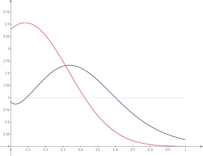
Figure 1: Stationary density of particles $\rho{st}$ in quadratic chemotaxis gradient $S(x)=5x$, on domain of $[0,1]$, calculated with anomalous substance $\nu(x)=\nu_{0}e^{-kx}$, $\nu_{0}=0.9$ and $k=2.19$. The blue line represent the density with no adhesion effects $\lambda_{\aleph}=\mu_{\alpha}=2\times 10^{-4}(1-\chi\rho_{st})$. The red line is the density where escape rates depend on the density of particles on the neighbours $\lambda_{\aleph}=2\times 10^{-4}(1-\chi\rho_{st,-1})$, and $\mu_{\aleph}=2\times 10^{-4}(1-\chi\rho_{st,+1})$, where $\chi=0.1$.

Conclusions

The main target in this work has been to implement adhesion effect, involving nonlinear dependence, into fractional subdiffusion transition model. We presented a non-Markovian and non-linear random walk model, where the escape rates inversely proportional to the residence time $\tau$, and they also depend on the density of particles at the neighbours. We derived the generalised master equation for this model, it included the exponential factor that involves the non-linear escape rate dependence with adhesion effects. In the subdiffusive case, the resulted master equation involved to a non-trivial combination of the non-linear exponential factor together with the Riemann-Liouville fractional derivative. This combination performs as a tempering to the anomalous trapping process. In long time limit, we could evaluate the fractional master equation in terms of stationary density. The stationary solution with non-linear dependence of $\alpha$ upon to $\rho$ led to a nonlinear advection and diffusion, which are both dependent on nonlinear escape rates with adhesion effects. Finally, we presented a numerical simulation for the stationary solution in figure (1), that showed that adhesion effects seemed to slow particles down and force them to aggregate. This Model can also be applied on transport systems with non-standard diffusion, where memory kernels causes a dependence between reactions and transport, like the case of propagating front [33].

Acknowledgement 1.

The author is very grateful to Prof. Sergei Fedotov for his great help and support.

References

• [1] Stephen Turner, Jonathan A. Sherratt, Kevin J. Painter and Nicholas J. Savill “From a discrete to a continuous model of biological cell movement” In Physical Review E 69.2, 2004, pp. 021910 DOI: 10.1103/PhysRevE.69.021910
• [2] Nicola J. Armstrong, Kevin J. Painter and Jonathan A. Sherratt “A continuum approach to modelling cell–cell adhesion” In Journal of Theoretical Biology 243.1, 2006, pp. 98–113 DOI: 10.1016/j.jtbi.2006.05.030
• [3] K. Anguige and C. Schmeiser “A one-dimensional model of cell diffusion and aggregation, incorporating volume filling and cell-to-cell adhesion” In Journal of Mathematical Biology 58.3, 2008, pp. 395–427 DOI: 10.1007/s00285-008-0197-8
• [4] Matthew J. Simpson, Chris Towne, D. L. Sean McElwain and Zee Upton “Migration of breast cancer cells: Understanding the roles of volume exclusion and cell-to-cell adhesion” In Physical Review E 82.4, 2010, pp. 041901 DOI: 10.1103/PhysRevE.82.041901
• [5] Matthew J. Simpson, Kerry A. Landman, Barry D. Hughes and Anthony E. Fernando “A model for mesoscale patterns in motile populations” In Physica A: Statistical Mechanics and its Applications 389.7, 2010, pp. 1412–1424 DOI: 10.1016/j.physa.2009.12.010
• [6] Stuart T. Johnston, Matthew J. Simpson and Ruth E. Baker “Mean-field descriptions of collective migration with strong adhesion” In Physical Review E 85.5, 2012, pp. 051922 DOI: 10.1103/PhysRevE.85.051922
• [7] Robin N. Thompson, Christian A. Yates and Ruth E. Baker “Modelling Cell Migration and Adhesion During Development” In Bulletin of Mathematical Biology 74.12, 2012, pp. 2793–2809 DOI: 10.1007/s11538-012-9779-0
• [8] Kevin Kendall “Molecular Adhesion and Its Applications” Boston: Kluwer Academic Publishers, 2004 URL: http://link.springer.com/10.1007/b100328
• [9] Haye Hinrichsen and Dietrich E. Wolf “The physics of granular media / Haye Hinrichsen and Dietrich E. Wolf.” Weinheim: Wiley-VCH, 2004
• [10] L Wolpert “Principles of development / Lewis Wolpert … [et al.].” Oxford ; New York: Oxford University Press, 2011
• [11] Ramsey A. Foty and Malcolm S. Steinberg “The differential adhesion hypothesis: a direct evaluation” In Developmental Biology 278.1, 2005, pp. 255–263 DOI: 10.1016/j.ydbio.2004.11.012
• [12] Radek Erban and Hans G. Othmer “From Individual to Collective Behavior in Bacterial Chemotaxis” In SIAM Journal on Applied Mathematics 65.2, 2004, pp. 361–391 URL: http://www.jstor.org/stable/4096270
• [13] Christophe Deroulers, Marine Aubert, Mathilde Badoual and Basil Grammaticos “Modeling tumor cell migration: From microscopic to macroscopic models” In Physical Review E 79.3, 2009, pp. 031917 DOI: 10.1103/PhysRevE.79.031917
• [14] Evgeniy Khain et al. “Collective behavior of brain tumor cells: The role of hypoxia” In Physical Review E 83.3, 2011, pp. 031920 DOI: 10.1103/PhysRevE.83.031920
• [15] STEPHEN TURNER and JONATHAN A. SHERRATT “Intercellular Adhesion and Cancer Invasion: A Discrete Simulation Using the Extended Potts Model” In Journal of Theoretical Biology 216.1, 2002, pp. 85–100 DOI: 10.1006/jtbi.2001.2522
• [16] Anthony E. Fernando, Kerry A. Landman and Matthew J. Simpson “Nonlinear diffusion and exclusion processes with contact interactions” In Physical Review E 81.1, 2010, pp. 011903 DOI: 10.1103/PhysRevE.81.011903
• [17] Catherine J. Penington, Barry D. Hughes and Kerry A. Landman “Building macroscale models from microscale probabilistic models: A general probabilistic approach for nonlinear diffusion and multispecies phenomena” In Physical Review E 84.4, 2011, pp. 041120 DOI: 10.1103/PhysRevE.84.041120
• [18] Alexander R. A. Anderson “A hybrid mathematical model of solid tumour invasion: the importance of cell adhesion” In Mathematical Medicine and Biology 22.2, 2005, pp. 163–186 DOI: 10.1093/imammb/dqi005
• [19] V. Mendez, S. Fedotov and W. Horsthemke “Reaction-Transport Systems: Mesoscopic Foundations, Fronts, and Spatial Instabilities” Springer, 2010
• [20] C. N. Angstmann, I. C. Donnelly and B. I. Henry “Continuous Time Random Walks with Reactions Forcing and Trapping” In Mathematical Modelling of Natural Phenomena 8.2, 2013, pp. 17–27 DOI: 10.1051/mmnp/20138202
• [21] S. Fedotov “Nonlinear subdiffusive fractional equations and the aggregation phenomenon” In Physical Review E 88.3, 2013, pp. 032104 DOI: 10.1103/PhysRevE.88.032104
• [22] P. Straka and S. Fedotov “Transport equations for subdiffusion with nonlinear particle interaction” In Journal of Theoretical Biology 366, 2015, pp. 71–83 DOI: 10.1016/j.jtbi.2014.11.012
• [23] S. Falconer, A. Al-Sabbagh and S. Fedotov “Nonlinear Tempering of Subdiffusion with Chemotaxis, Volume Filling, and Adhesion” In Mathematical Modelling of Natural Phenomena 10.3, 2015, pp. 48–60 DOI: 10.1051/mmnp/201510305
• [24] T. Hillen and K. Painter “Global Existence for a Parabolic Chemotaxis Model with Prevention of Overcrowding” In Advances in Applied Mathematics 26.4, 2001, pp. 280–301 DOI: 10.1006/aama.2001.0721
• [25] T. Hillen and K. J. Painter “A user’s guide to PDE models for chemotaxis” In Journal of Mathematical Biology 58.1-2, 2008, pp. 183–217 DOI: 10.1007/s00285-008-0201-3
• [26] M. O. Vlad and J. Ross “Systematic derivation of reaction-diffusion equations with distributed delays and relations to fractional reaction-diffusion equations and hyperbolic transport equations: Application to the theory of Neolithic transition” In Physical Review E 66.6, 2002, pp. 061908 DOI: 10.1103/PhysRevE.66.061908
• [27] A. Yadav and W. Horsthemke “Kinetic equations for reaction-subdiffusion systems: Derivation and stability analysis” In Physical Review E 74.6, 2006, pp. 066118 DOI: 10.1103/PhysRevE.74.066118
• [28] S. Fedotov “Subdiffusion, chemotaxis, and anomalous aggregation” In Physical Review E 83.2, 2011, pp. 021110 DOI: 10.1103/PhysRevE.83.021110
• [29] S. Fedotov and S. Falconer “Subdiffusive master equation with space-dependent anomalous exponent and structural instability” In Physical review. E, Statistical, nonlinear, and soft matter physics 85.3 Pt 1, 2012, pp. 031132
• [30] S. Fedotov, A. O. Ivanov and A. Y. Zubarev “Non-homogeneous Random Walks, Subdiffusive Migration of Cells and Anomalous Chemotaxis” In Mathematical Modelling of Natural Phenomena 8.02, 2013, pp. 28–43 DOI: 10.1051/mmnp/20138203
• [31] S. Fedotov and S. Falconer “Nonlinear degradation-enhanced transport of morphogens performing subdiffusion” In Physical Review E 89.1, 2014, pp. 012107 DOI: 10.1103/PhysRevE.89.012107
• [32] S. Fedotov and N. Korabel “Subdiffusion in an external potential: Anomalous effects hiding behind normal behavior” In Physical Review E 91.4, 2015, pp. 042112 DOI: 10.1103/PhysRevE.91.042112
• [33] A. Yadav, S. Fedotov, V. Méndez and W. Horsthemke “Propagating fronts in reaction–transport systems with memory” In Physics Letters A 371.5, 2007, pp. 374–378 DOI: 10.1016/j.physleta.2007.06.044