Sulphur molecules in the circumstellar envelopes of M-type AGB stars

Abstract

Aims. The sulphur compounds SO and $\mathrm{SO}_{2}$ have not been widely studied in the circumstellar envelopes of asymptotic giant branch (AGB) stars. By presenting and modelling a large number of SO and $\mathrm{SO}_{2}$ lines in the low mass-loss rate M-type AGB star R Dor, and modelling the available lines of those molecules in a further four M-type AGB stars, we aim to determine their circumstellar abundances and distributions.

Methods. We use a detailed radiative transfer analysis based on the accelerated lambda iteration method to model circumstellar SO and $\mathrm{SO}_{2}$ line emission. We use molecular data files for both SO and $\mathrm{SO}_{2}$ that are more extensive than those previously available.

Results. Using 17 SO lines and 98 $\mathrm{SO}_{2}$ lines to constrain our models for R Dor, we find an SO abundance of $(6.7\pm 0.9)\times 10^{-6}$ and an $\mathrm{SO}_{2}$ abundance of $5\times 10^{-6}$ with both species having high abundances close to the star. We also modelled ³⁴SO and found an abundance of $(3.1\pm 0.8)\times 10^{-7}$, giving an ³²SO/³⁴SO ratio of $21.6\pm 8.5$. We derive similar results for the circumstellar SO and $\mathrm{SO}_{2}$ abundances and their distributions for the low mass-loss rate object W Hya. For the higher mass-loss rate stars, we find shell-like SO distributions with peak abundances that decrease and peak abundance radii that increase with increasing mass-loss rate. The positions of the peak SO abundance agree very well with the photodissociation radii of $\mathrm{H}_{2}$O. We also modelled $\mathrm{SO}_{2}$ in two higher mass-loss rate stars but our models for these were less conclusive.

Conclusions. We conclude that for the low mass-loss rate stars, the circumstellar SO and $\mathrm{SO}_{2}$ abundances are much higher than predicted by chemical models of the extended stellar atmosphere. These two species may also account for all the available sulphur. For the higher mass-loss rate stars we find evidence that SO is most efficiently formed in the circumstellar envelope, most likely through the photodissociation of $\mathrm{H}_{2}$O and the subsequent reaction between S and OH. The S-bearing parent molecule does not appear to be $\mathrm{H}_{2}$S. The $\mathrm{SO}_{2}$ models for the higher mass-loss rate stars are less conclusive, but suggest an origin close to the star for this species. This is not consistent with current chemical models. The combined circumstellar SO and $\mathrm{SO}_{2}$ abundances are significantly lower than that of sulphur for these higher mass-loss rate objects.

1 Introduction

Low- to intermediate-mass stars eventually evolve from the main sequence to the asymptotic giant branch (AGB). AGB stars lose mass rapidly, producing a circumstellar envelope (CSE) of atomic and molecular matter and dust, rich in chemical diversity. The variety and abundances of molecules that can be found in the circumstellar envelopes of AGB stars depend on the chemistry of the individual star. For example, carbon stars, which have carbon-to-oxygen ratio C/O $>1$, are most likely to have a variety of C-bearing molecules in their CSEs (e.g. Gong et al., 2015), while oxygen-rich M-type stars, with C/O $<1$, are more likely to contain a variety of O-bearing molecules (e.g. Justtanont et al., 2012).

SO and $\mathrm{SO}_{2}$ are two such O-bearing molecules. They are thought to exist in shells in the CSE, having been formed through the photodissociation of the parent molecule $\mathrm{H}_{2}$S and subsequent reactions with O and OH (Cherchneff, 2006; Willacy & Millar, 1997). Observations of the red supergiant VY CMa by Adande et al. (2013) contradict this view, however; the modelling results show small, concentrated envelopes of SO and $\mathrm{SO}_{2}$ and indications that $\mathrm{SO}_{2}$ may itself be formed directly, rather than being a photodissociation product of $\mathrm{H}_{2}$S or another molecule and are found in a hollow shell around the star. Similarly, when Decin et al. (2010a) modelled $\mathrm{SO}_{2}$ emission around the AGB star IK Tau, they had difficulty reconciling their observations with a shell model.

The Yamamura et al. (1999) ISO/SWS detections of the 7.4 $\mathrm{}\mu\mathrm{m}$ $\nu_{3}$ $\mathrm{SO}_{2}$ band in a few AGB stars suggest that $\mathrm{SO}_{2}$ is formed in the warmest regions of the CSE. Analysis of these data by Yamamura et al. (1999) and Cami et al. (1999) indicates that the $\mathrm{SO}_{2}$ is mostly likely formed within a few stellar radii of the star at a temperature of $\sim$ 600 K. Cami et al. (1999) also find that the excitation of $\mathrm{SO}_{2}$ to the $\nu_{3}$ band varies with pulsation period. Their simple models put the outer radius of $\mathrm{SO}_{2}$ within $\sim 5R_{*}$.

In this paper we present new observations of circumstellar SO and $\mathrm{SO}_{2}$ from an APEX spectral survey of the M-type AGB star R Dor. We combine these results with SO and $\mathrm{SO}_{2}$ detections from Herschel/HIFI, developing comprehensive models of the SO and $\mathrm{SO}_{2}$ distributions around R Dor using 17 SO lines and 98 $\mathrm{SO}_{2}$ lines, all spectrally resolved.

We also model the sparse detections of SO and $\mathrm{SO}_{2}$ emission towards the other M-type AGB stars observed with Herschel/HIFI, supplemented with archival data where available.

2 Sample and observations

The stars included in this study come from the sample of M-type AGB stars observed as part of the HIFISTARS Guaranteed Time Key Programme (Justtanont et al., 2012, and see Sect. 2.2 for details). The OH/IR stars are excluded, as is Mira, which has a complicated and asymmetric CSE induced by a white dwarf companion (see Ramstedt et al., 2014). That leaves a sample of five M-stars, four of which had SO and $\mathrm{SO}_{2}$ lines detected by HIFI. The remaining star, TX Cam, has previously been detected in SO at lower frequencies.

Some basic information about the five sources is given in Table 1.

Table 1: Basic information about our five sources.

Star	RA	Dec	Variability	Spec type
IK Tau	03 53 28.87	$+$11 24 21.7	M	M9
R Dor	04 36 45.59	$-$62 04 37.8	SRB	M8e
TX Cam	05 00 50.39	$+$56 10 52.6	M	M8.5
W Hya	13 49 02.00	$-$28 22 03.5	M	M7.5-9e
R Cas	23 58 24.87	$+$51 23 19.7	M	M6.5-9e

2.1 APEX data

We performed a spectral survey of R Dor in the ranges $213-321.5$ GHz and $338.5-368.5$ GHz ($\lambda=0.8-1.4$ mm) using the Swedish Heterodyne Facility Instrument (SHeFI; Vassilev et al., 2008) on the Atacama Pathfinder Experiment telescope (APEX). The data were observed over several observing seasons between May 2011 and June 2015. The observations were carried out using beam switching with a standard beam throw of 3′. A detailed description of this survey will be presented by De Beck et al., (in prep.).

Data reduction was carried out using the Gildas/Class package. Scans with very unstable baselines were ignored and bad channels were blanked. After masking the regions with line emission, polynomial baselines of typically first degree were subtracted from the averaged spectra to obtain a 0 K baseline. Rms noise levels throughout the survey are around $2-10$ mK at a velocity resolution of 1 km s^-1. The spectra were then converted to main beam temperatures using efficiency correction factors of $\eta_{mb}=0.75$ for $\nu<270$ GHz, $\eta_{mb}=0.74$ for $270<\nu<320$ GHz, and $\eta_{mb}=0.73$ for $\nu>320$ GHz. The half-power beam-widths were calculated using the general formula

$$\theta=7.8\left(\frac{800}{\nu}\right)$$ (1)

where $\nu$ is in GHz and $\theta$ is in arcseconds. The beam-widths across our frequency range are between 17–29$\arcsec$.

The detections of SO using APEX are listed in Table 2 and the $\mathrm{SO}_{2}$ detections are listed in Table 3. There were also some detections of SO and $\mathrm{SO}_{2}$ isotopologues: ³⁴SO, and tentative detections of ³⁴$\mathrm{SO}_{2}$ and SO¹⁸O. We model ³⁴SO, but are unable to perform a full radiative transfer analysis for the other isotopologues. See Table 4 for a list of isotopologue detections and for the full discussion, see Sect. 3.2.4.

In terms of other S-bearing molecules, there were no conclusive detections of either CS (out of three possible transitions in the range $J_{\mathrm{up}}=5$ to $J_{\mathrm{up}}=7$) or SiS (out of nine possible transitions in the range $J_{\mathrm{up}}=12$ to $J_{\mathrm{up}}=20$). There was a tentative detection of CS ($6\to 5$) but it is blended with ²⁹SiO($7\to 6$, $v=3$) line and hence allows no reliable conclusion on the detection of CS. (We note that there are several other detections of ²⁹SiO in the survey, but none of CS.) No other S-bearing molecules were detected in this survey.

Table 2: SO observations towards R Dor using APEX, listed in order of descending energy of the upper level.

Transition	$\nu\;\;\;$	$E_{\mathrm{up}}$	$\theta\;$	$I_{mb}$
	[GHz]	[K]	[″]	[K $\mathrm{km\,s}^{-1}$]
$8_{8}\to 7_{7}$	344.311	88	18	5.04
$8_{7}\to 7_{6}$	340.714	81	18	4.59
$8_{9}\to 7_{8}$	$\dagger$ 346.528	79	18	4.54
$7_{7}\to 6_{6}$	301.286	71	21	4.74
$7_{6}\to 6_{5}$	296.550	65	21	4.12
$7_{8}\to 6_{7}$	304.078	62	21	6.40
$6_{6}\to 5_{5}$	258.256	57	24	3.49
$6_{5}\to 5_{4}$	251.826	51	25	3.13
$6_{7}\to 5_{6}$	261.844	48	24	5.20
$5_{5}\to 4_{4}$	215.221	44	29	2.25
$5_{6}\to 4_{5}$	219.949	35	28	4.21
$3_{3}\to 2_{3}$	339.341	26	18	00.125
$2_{2}\to 1_{2}$	309.502	19	20	00.100

Table 3: SO₂ observations towards R Dor using APEX, listed in order of descending energy of the upper level.

Transition	$\nu\;\;\;$	$E_{\mathrm{up}}$	$\theta\;$	$I_{mb}$	Transition	$\nu\;\;\;$	$E_{\mathrm{up}}$	$\theta\;$	$I_{mb}$
	[GHz]	[K]	[″]	[K $\mathrm{km\,s}^{-1}$]		[GHz]	[K]	[″]	[K $\mathrm{km\,s}^{-1}$]
$25_{4,22}\to 26_{1,25}$	* 279.497	1085	22	0.373	$16_{3,13}\to 16_{2,14}$	214.689	148	29	0.415
$40_{4,36}\to 40_{3,37}$	341.403	808	18	0.217	$17_{1,17}\to 16_{0,16}$	313.661	136	20	2.881
$36_{5,31}\to 36_{4,32}$	341.674	679	18	0.148	$14_{4,10}\to 14_{3,11}$	351.874	136	18	0.860
$36_{4,32}\to 36_{3,33}$	281.689	662	22	0.257	$15_{3,13}\to 15_{2,14}$	275.240	133	23	0.745
$34_{5,29}\to 34_{4,30}$	360.290	612	17	0.250	$16_{1,15}\to 15_{2,14}$	236.217	131	26	0.595
$34_{3,31}\to 34_{2,32}$	342.762	582	18	0.255	$13_{4,10}\to 13_{3,11}$	357.165	123	17	0.919
$32_{4,28}\to 32_{3,29}$	258.389	531	24	0.368	$16_{0,16}\to 15_{1,15}$	283.292	121	22	0.959
$32_{3,29}\to 32_{2,30}$	300.273	519	21	0.453	$15_{2,14}\to 15_{1,15}$	248.057	119	25	0.423
$30_{4,26}\to 30_{3,27}$	259.599	472	24	0.212	$15_{2,14}\to 14_{1,13}$	366.214	119	17	0.840
$30_{3,27}\to 30_{2,28}$	263.544	459	24	0.231	$14_{3,11}\to 14_{2,12}$	226.300	119	28	0.596
$28_{4,24}\to 28_{3,25}$	267.720	416	23	0.412	$12_{4,8}\to 12_{3,9}$	355.046	111	18	0.498
$28_{3,25}\to 28_{2,26}$	234.187	403	27	0.289	$13_{3,11}\to 13_{2,12}$	267.537	106	23	0.600
$28_{3,25}\to 27_{4,24}$	$\dagger$ 313.412	403	20	0.129	$15_{1,15}\to 14_{0,14}$	281.763	107	22	2.007
$28_{2,26}\to 28_{1,27}$	340.316	392	18	0.365	$11_{4,8}\to 11_{3,9}$	357.388	100	17	0.980
$26_{4,22}\to 26_{3,23}$	280.807	364	22	0.382	$12_{3,9}\to 12_{2,10}$	237.069	94	26	0.616
$26_{3,23}\to 26_{2,24}$	213.068	351	29	0.410	$14_{0,14}\to 13_{1,13}$	244.254	94	26	1.702
$26_{3,23}\to 25_{4,22}$	245.339	351	25	0.216	$13_{2,12}\to 13_{1,13}$	225.154	93	28	0.652
$26_{2,24}\to 26_{1,25}$	296.169	341	21	0.306	$13_{2,12}\to 12_{1,11}$	$\dagger$ 345.339	93	18	2.283
$25_{3,23}\to 25_{2,24}$	359.151	321	17	0.601	$10_{4,6}\to 10_{3,7}$	356.755	90	17	0.804
$24_{4,20}\to 24_{3,21}$	$\dagger$ 296.535	317	21	0.520	$11_{3,9}\to 11_{2,10}$	262.257	83	24	0.639
$24_{1,23}\to 24_{0,24}$	363.891	281	17	0.396	$13_{1,13}\to 12_{0,12}$	$\dagger$ 251.200	82	25	1.275
$22_{4,18}\to 22_{3,19}$	312.543	273	20	0.424	$9_{4,6}\to 9_{3,7}$	357.672	81	17	0.497
$23_{2,22}\to 23_{1,23}$	363.926	260	17	0.741	$10_{3,7}\to 10_{2,8}$	245.563	73	25	0.587
$21_{4,18}\to 21_{3,19}$	363.159	252	17	0.815	$8_{4,4}\to 8_{3,5}$	357.581	72	17	0.686
$22_{2,20}\to 22_{1,21}$	216.643	248	29	0.373	$7_{4,4}\to 7_{3,5}$	357.892	65	17	0.685
$22_{2,20}\to 21_{3,19}$	286.416	248	22	0.168	$9_{3,7}\to 9_{2,8}$	258.942	64	24	0.561
$21_{3,19}\to 21_{2,20}$	316.099	235	20	0.878	$11_{1,11}\to 10_{0,10}$	221.965	60	28	0.953
$19_{4,16}\to 19_{3,17}$	359.771	214	17	0.430	$6_{4,2}\to 6_{3,3}$	357.926	59	17	0.527
$20_{1,19}\to 20_{0,20}$	282.293	199	22	0.751	$8_{3,5}\to 8_{2,6}$	$\dagger$ 251.211	55	25	0.995
$20_{1,19}\to 19_{2,18}$	338.612	199	18	1.255	$5_{4,2}\to 5_{3,3}$	358.013	53	17	0.398
$19_{3,17}\to 19_{2,18}$	299.317	197	21	0.496	$9_{2,8}\to 8_{1,7}$	298.576	51	21	0.496
$20_{0,20}\to 19_{1,19}$	$\dagger$ 358.216	185	17	2.373	$4_{4,0}\to 4_{3,1}$	358.038	49	17	0.234
$19_{2,18}\to 19_{1,19}$	301.897	183	21	0.561	$7_{3,5}\to 7_{2,6}$	257.100	48	24	0.448
$17_{4,14}\to 17_{3,15}$	357.963	180	17	0.917	$6_{3,3}\to 6_{2,4}$	$\dagger$ 254.281	41	25	0.776
$19_{1,19}\to 18_{0,18}$	346.652	168	18	1.390	$5_{3,3}\to 5_{2,4}$	256.247	36	24	0.350
$16_{4,12}\to 16_{3,13}$	$\dagger$ 346.524	165	18	3.864	$5_{3,3}\to 4_{2,2}$	351.257	36	18	0.705
$18_{1,17}\to 18_{0,18}$	240.943	163	26	0.506	$7_{2,6}\to 6_{1,5}$	271.529	36	23	0.426
$18_{1,17}\to 17_{2,16}$	288.520	163	22	0.852	$4_{3,1}\to 4_{2,2}$	255.553	31	24	0.215
$17_{3,15}\to 17_{2,16}$	285.744	163	22	0.382	$6_{2,4}\to 5_{1,5}$	282.037	29	22	0.349
$18_{0,18}\to 17_{1,17}$	321.330	152	19	2.091	$3_{3,1}\to 2_{2,0}$	313.280	28	20	0.381
$15_{4,12}\to 15_{3,13}$	357.241	150	17	0.893	$5_{2,4}\to 4_{1,3}$	241.616	24	26	0.398
$17_{2,16}\to 17_{1,17}$	273.753	149	23	0.378	$4_{2,2}\to 3_{1,3}$	235.152	19	27	0.211

Table 4: SO and $\mathrm{SO}_{2}$ isotopologue observations towards R Dor using APEX.

	Transition	$\nu\;\;\;$	$E_{\mathrm{up}}$	$\theta\;$	$I_{mb}$
		[GHz]	[K]	[″]	[K $\mathrm{km\,s}^{-1}$]
34SO	$8_{9}\to 7_{8}$	339.857	77.3	18	0.26
	$7_{7}\to 6_{6}$	295.396	69.9	21	0.20
	$7_{8}\to 6_{7}$	298.258	61.1	21	0.42
	$6_{6}\to 5_{5}$	253.207	55.7	25	0.26
	$6_{7}\to 5_{6}$	256.878	46.7	24	0.38
	$5_{6}\to 4_{5}$	215.840	34.4	29	0.18
34SO2	$20_{0,20}\to 19_{1,19}$	357.102	184.6	17	0.25
	$17_{3,15}\to 17_{2,16}$	279.075	161.9	22	0.11
	$6_{3,3}\to 5_{2,4}$	362.158	40.6	17	0.24
SO18O	$35_{10,26}\to 36_{9,27}$	288.482	786.3	22	0.19
	$19_{3,17}\to 19_{2,18}$	288.270	186.8	22	0.24
	$18_{0,18}\to 17_{1,17}$	303.476	143.4	21	0.18
	$17_{2,16}\to 16_{2,15}$	303.155	141.3	21	0.28
	$14_{4,10}\to 14_{3,11}$	344.874	129.6	18	0.24

2.2 HIFI data

R Dor, IK Tau, R Cas, TX Cam and W Hya were observed as part of the HIFISTARS Guaranteed Time Key Programme, using the Herschel/HIFI instrument (de Graauw et al., 2010) to observe emission lines with high spectral resolution. The full results are presented in detail in Justtanont et al. (2012). Since those data were published, there have been updates to the main beam efficiencies (Mueller et al., 2014) and for this work we have re-reduced the HIFI data to take this into account (using HIPE version 12.1, Ott, 2010). We have also identified three additional $\mathrm{SO}_{2}$ lines that were not included in Justtanont et al. (2012). The detected SO and $\mathrm{SO}_{2}$ HIFI lines are listed in Table 5. We note that no SO or $\mathrm{SO}_{2}$ lines were detected with HIFI in TX Cam.

Table 5: SO₂ and SO observations using HIFI, listed by molecule in order of descending energy of the upper level.

Molecule	Transition	$\nu\;\;\;$	$E_{\mathrm{up}}$	$\theta\;$	IK Tau	R Dor	TX Cam	W Hya	R Cas
		[GHz]	[K]	[″]	[K $\mathrm{km\,s}^{-1}$]	[K $\mathrm{km\,s}^{-1}$]	[K $\mathrm{km\,s}^{-1}$]	[K $\mathrm{km\,s}^{-1}$]	[K $\mathrm{km\,s}^{-1}$]
SO	$23_{24}\to 22_{23}$	988.618	575	21	-	-	-	0.76	-
	$15_{16}\to 14_{15}$	645.875	253	33	-	1.5	$<$0.1	0.43	0.13
	$13_{13}\to 12_{12}$	559.319	201	37	0.16	1.3	$<$0.08	0.55	0.16
	$13_{12}\to 12_{11}$	558.087	195	37	0.44	1.4	$<$0.08	0.42	0.14
	$13_{14}\to 12_{13}$	560.178	193	37	0.23	1.5	$<$0.08	0.58	0.26
SO2	$36_{2,34}\to 35_{3,33}$	* 661.510	630	32	-	0.37	-	-	-
	$37_{1,37}\to 36_{0,36}$	659.421	609	32	-	0.68	-	0.12	-
	$36_{1,35}\to 35_{2,34}$	658.632	606	32	0.16	0.61	-	0.35	0.26
	$32_{2,30}\to 31_{3,29}$	571.532	505	36	-	1 0.20 $\dagger$	-	-	-
	$27_{7,21}\to 27_{6,22}$	* 657.885	468	32	-	0.21	-	-	-
	$32_{0,32}\to 31_{1,31}$	571.553	459	36	-	1 0.39 $\dagger$	-	-	-
	$25_{7,19}\to 25_{6,20}$	* 659.338	419	32	-	0.25	-	-	-
	$24_{7,17}\to 24_{6,18}$	659.898	396	32	-	1 0.23 $\dagger$	-	-	-
	$23_{7,17}\to 22_{6,16}$	1102.115	374	19	-	0.93	-	-	-
	$22_{6,16}\to 22_{5,17}$	557.283	321	37	-	0.29	-	0.14	-
	$15_{9,7}\to 14_{8,6}$	1151.852	309	19	-	1.50	-	-	-
	$21_{6,16}\to 21_{5,17}$	558.391	301	37	-	0.22	-	0.20	-
	$13_{9,5}\to 12_{8,4}$	1113.506	282	19	-	0.76	-	-	-
	$20_{6,14}\to 20_{5,15}$	558.812	282	37	-	0.14	-	-	-
	$18_{6,12}\to 18_{5,13}$	559.882	246	37	-	0.19	-	0.12	-
	$16_{6,10}\to 16_{5,11}$	560.613	213	37	-	0.22	-	-	-

2.3 Archival data

To supplement the HIFI data for IK Tau, R Cas, W Hya, and TX Cam, we have used observations found in the literature. These are listed in Table 6. As the older data generally covers lower-energy transitions than those observed by HIFI, we are better able to constrain our models over a larger energy range. This is particularly important for R Cas, IK Tau and TX Cam where the HIFI lines (or non-detections in the case of TX Cam) are clustered close together energetically.

Table 6: Archival observations of SO and $\mathrm{SO}_{2}$ towards IK Tau, TX Cam, R Cas, and W Hya.

Source	Molecule	Transition	$\nu$	$E_{\mathrm{up}}$	Telescope	$\theta$	$I_{mb}$	Reference
			[GHz]	[K]		[″]	[K $\mathrm{km\,s}^{-1}$]
IK Tau	SO	$8_{8}\to 7_{7}$	344.310	88	APEX	18	2.7	Kim et al. (2010)
		$7_{7}\to 6_{6}$	301.286	71	APEX	20	0.89	Kim et al. (2010)
		$5_{6}\to 4_{5}$	219.949	35	NRAO	30	6.5	Sahai & Wannier (1992)
		$2_{2}\to 1_{1}$	86.094	19	IRAM	27	0.65	Omont et al. (1993)
		$3_{4}\to 2_{3}$	138.179	16	IRAM	17	13.5	Sahai & Wannier (1992)
		$2_{3}\to 1_{2}$	99.300	9	OSO	37.5	4.2	Sahai & Wannier (1992)
		$2_{3}\to 1_{2}$	99.300	9	OSO	37.5	3.6	Olofsson et al. (1998)
	SO2	$17_{1,17}\to 16_{0,16}$	313.660	136	APEX	20	11.3	Kim et al. (2010)
		$14_{4,10}\to 14_{3,11}$	351.873	136	APEX	18	0.55	Kim et al. (2010)
		$14_{3,11}\to 14_{2,12}$	226.300	119	IRAM	10.5	1.0	Decin et al. (2010a)
		$13_{2,12}\to 12_{1,11}$	345.338	93	APEX	18	6.3	Kim et al. (2010)
		$10_{1,9}\to 10_{0,10}$	104.239	55	IRAM	24	1.83	Omont et al. (1993)
		$10_{0,10}\to 9_{1,9}$	160.828	50	IRAM	15	8.6	Omont et al. (1993)
		$5_{3,3}\to 5_{2,4}$	256.247	36	IRAM	9.5	3.4	Decin et al. (2010a)
		$5_{3,3}\to 4_{2,2}$	351.257	36	APEX	18	1.4	Kim et al. (2010)
		$4_{3,1}\to 4_{2,2}$	255.553	31	IRAM	9.5	3.2	Decin et al. (2010a)
		$4_{3,1}\to 3_{2,2}$	332.505	31	APEX	19	1.4	Kim et al. (2010)
		$3_{3,1}\to 3_{2,2}$	255.958	28	IRAM	9.5	2.2	Decin et al. (2010a)
		$3_{3,1}\to 2_{2,0}$	313.279	28	APEX	20	2.2	Kim et al. (2010)
		$3_{1,3}\to 2_{0,2}$	104.029	8	IRAM	24	1.78	Omont et al. (1993)
TX Cam	SO	$5_{6}\to 4_{5}$	219.949	35	IRAM	13	7.0	Bujarrabal et al. (1994)
		$5_{6}\to 4_{5}$	219.949	35	NRAO	30	1.8	Sahai & Wannier (1992)
		$2_{3}\to 1_{2}$	99.300	9	OSO	37.5	2.9	Sahai & Wannier (1992)
		$2_{3}\to 1_{2}$	99.300	9	OSO	37.5	2.1	Olofsson et al. (1998)
W Hya	SO	$5_{5}\to 4_{4}$	215.221	31	SMA	1.5	*8.2*	Vlemmings et al. (2011)
		$2_{3}\to 1_{2}$	99.300	9	SEST	51	0.2	Olofsson et al. (1998)
R Cas	SO	$5_{6}\to 4_{5}$	219.949	35	NRAO	30	2.0	Sahai & Wannier (1992)
		$2_{3}\to 1_{2}$	99.300	9	OSO	37.5	1.4	Sahai & Wannier (1992)
		$2_{3}\to 1_{2}$	99.300	9	OSO	37.5	1.7	Olofsson et al. (1998)
	SO2	$3_{1,3}\to 2_{0,2}$	104.029	7.7	IRAM	24	0.81	Guilloteau et al. (1986)

3 Modelling

3.1 Modelling procedure

We perform detailed radiative transfer modelling of the molecular emission lines using an accelerated lambda iteration method code (ALI), which has been previously described and implemented by e.g. Maercker et al. (2008); Schöier et al. (2011); Danilovich et al. (2014). ALI is particularly useful in this work as it is able to take into account extensive descriptions of molecular properties — such as large numbers of energy levels and transitions — while still fully solving the statistical equilibrium equations and taking temperature and velocity profiles into account.

We assume a smoothly expanding spherical CSE produced by a constant mass-loss rate. The molecules are located in this CSE until they eventually become photodissociated. They are excited by collisions with $\mathrm{H}_{2}$ molecules and through radiation from the star, the dust, and the cosmic microwave background. ALI input parameters such as the kinetic temperature distribution, dust temperature, and dust optical depth, are taken from CO modelling and, where applicable, are listed in Table 7. For R Dor, R Cas, IK Tau, and TX Cam Maercker et al. (in prep.) performed detailed radiative transfer modelling of the CO and $\mathrm{H}_{2}$O lines and we use their results in our modelling. We based our CO model of W Hya on the results of Khouri et al. (2014a), but generated a CO model using the same code as in Maercker et al. (in prep.) for consistency between the stars.

We calculated the best fit model for each star and molecule using a $\chi^{2}$ statistic, which we define as

$$\chi^{2}=\sum^{N}_{i=1}\frac{(I_{\mathrm{mod},i}-I_{\mathrm{obs},i})^{2}}{\sigma_{i}^{2}}$$ (2)

where $I$ is the integrated line intensity, $\sigma$ is the uncertainty in the observations, and $N$ is the number of lines being modelled. We also calculate a reduced $\chi^{2}$ value such that $\chi^{2}_{\mathrm{red}}=\chi^{2}/(N-p)$ where $p$ is the number of free parameters.

After testing both centrally-peaked and shell-like abundance distributions, we came to the conclusion that the best radial abundance distribution profiles for both SO and $\mathrm{SO}_{2}$ in R Dor and W Hya were Gaussian profiles of the form

$$f=f_{p}\exp\left(-\left(\frac{r}{R_{e}}\right)^{2}\right)$$ (3)

where $f_{p}$ is the peak abundance at the inner radius, and $R_{e}$ is the $e$-folding radius, the radius at which the abundance has dropped by a factor of $1/e$.

In the cases of IK Tau and R Cas, we found that a shell model was a better fit to the observed SO lines. As such, we modelled IK Tau and R Cas assuming a Gaussian shell for the abundance distribution of the form

$$f=f_{p}\exp\left(-4\frac{(r-R_{p})^{2}}{R_{w}^{2}}\right)$$ (4)

where $f_{p}$ is the peak abundance, $R_{p}$ is the radial distance of the peak of the distribution from the centre of the star, and $R_{w}$, is the width of the shell at the $e$-folding radius. Using a shell distribution for both IK Tau and R Cas rather than a central Gaussian distribution significantly improved the $\chi^{2}$ fits of the models.

Similarly, we can firmly rule out a centrally-peaked model for TX Cam, as for such a model to fit the archival data we would expect conclusive detections in the HIFI data. As the undetected HIFI lines are of higher energy than the archival detections, a lower abundance in the inner regions of the CSE is expected, than in the outer regions, which points to a shell-like abundance distribution.

3.1.1 SO

For the radiative transfer analysis of SO we include 182 rotational energy levels, denoted $N_{J}$, up to $N=30$ in the ground and first excited vibrational states. There are 907 radiative transitions. These include pure rotational transitions in the $X^{3}\Sigma^{-}$ $v=0$ and $v=1$ states as well as the $v=1\to 0$ rovibrational lines. There are 8629 collisional transitions including collisions between all rotational states within a vibrational state, as well as between vibrational states. The rotational energy levels, transition frequencies, and A-values have been adapted directly from the CDMS (Müller et al., 2001, 2005). The infrared line list has been computed directly from the rotational levels with the band-head frequency adjusted to give very good agreement with the line positions measured by Burkholder et al. (1987). The vibration-rotation line strengths have been computed in intermediate coupling and have been verified by comparison with the pure rotational line strengths in the CDMS tables. The vibration-rotation transition dipole moment has been taken to be 0.08843 Debye, which yields inverse lifetimes of $A_{\mathrm{tot}}=3.6$ s^-1 for the $v=1\to 0$ band as computed by Peterson & Woods (1990). The collisional rate coefficients for pure rotational transitions were adapted from the He-SO rates computed by Lique et al. (2006) with mass-scaling to H₂ as in the smaller data set in the LAMDA database (Schöier et al., 2005). Rates for transitions within $v=1$ were assumed to be identical to those within $v=0$. Crude collision rates for $v=1\to 0$ were scaled in proportion to normalised radiative line strengths for electric-dipole-allowed transitions, with the largest values of the order of $1\times 10^{-11}$ cm³ s^-1.

In Fig. 1 we include an energy level diagram for SO. Here we have indicated all the transitions of SO detected towards R Dor with HIFI and APEX. These cover most of the transitions also detected in IK Tau, R Cas, W Hya, and TX Cam.

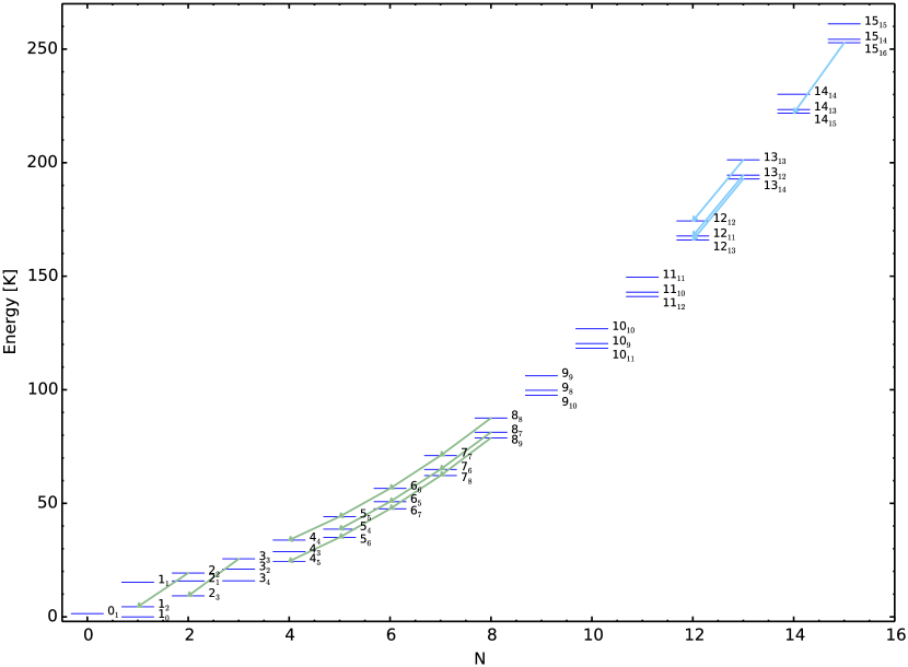
Figure 1: SO energy level diagram with levels labelled using the $N_{J}$ convention. Transitions detected with HIFI and APEX towards R Dor are indicated in light blue and green, respectively.

For the purposes of modelling the ³⁴SO emission in R Dor, we used a simpler molecular description than that for ³²SO, including the rotational energy levels up to $N=30$, corresponding to those included for ³²SO, but only in the ground vibrational state. When adopting the corresponding simpler molecular description for ³²SO in the case of R Dor specifically, we found that the final best fit model only shifted by a few percent between the detailed and simpler descriptions, justifying this approach for ³⁴SO. There was, however, some shift in final model for the other, especially higher mass-loss rate, stars when changing between the detailed and simpler molecular description for SO.

3.1.2 SO₂

Our radiative transfer analysis of $\mathrm{SO}_{2}$ includes 2600 energy levels, denoted $J_{Ka,Kc}$, across the ground vibrational state and the $\nu_{1}=1$ (8.7 $\mathrm{}\mu\mathrm{m}$), $\nu_{2}=1$ (19.3 $\mathrm{}\mu\mathrm{m}$) and $\nu_{3}=1$ (7.3 $\mathrm{}\mu\mathrm{m}$) vibrationally excited states. Levels with energies up to 4830 K and $J=38$ were included. This gives 15243 radiative transitions, with spectroscopic data taken from the HITRAN database (Rothman et al., 2013), and 15244 collisional transitions. The collision rates in the literature for SO₂ are inadequate for our purposes. Green (1995) calculated rate coefficients for He-SO₂ collisions in the infinite-order sudden approximation for the lowest 50 rotational levels (up to 100 K excitation energy and $J\leq 13$ only). Cernicharo et al. (2011) published rates for H₂-SO₂ collisions for the lowest 31 rotational levels at low temperatures, 5 to 30 K. The rates for H₂ impact were found to be approximately 10 times higher than corresponding rates for He impact. For the much larger number of states in our models, we adopted instead a set of crude collision rates in which the downward rate coefficient is proportional to the radiative line strength and normalised to a total collisional quenching rate of $2.0\times 10^{-10}$ cm³ s^-1, which is comparable to the highest collision rates found by Cernicharo et al. (2011). We tested the impact of the chosen collisional transition rates by multiplying the rates, in stages, by up to two orders of magnitude in both directions. We find that such drastic changes had only a very small and barely detectable effect on the resulting models. Hence we conclude that $\mathrm{SO}_{2}$ excitation is radiatively dominated with the choice of collisional transition rates playing only a minor role in the radiative transfer modelling.

In Fig. 2 we include an energy level diagram for $\mathrm{SO}_{2}$. Here we have indicated all transitions of $\mathrm{SO}_{2}$ detected towards R Dor with HIFI and APEX. As can be seen, $\mathrm{SO}_{2}$ has many close energy levels. This leads to a multitude of overlapping transitions, especially in AGB winds with typical expansion velocities of 5 – 25 $\mathrm{km\,s}^{-1}$. The number of levels, transitions and overlaps presents some computational challenges, especially when it comes to fully taking overlapping lines into account or running exhaustive grids. To reduce running time to a manageable interval we restrict the overlaps so that only those within the sampled frequency range, between 200 – 1200 GHz, are included. This reduced the total number of overlaps by more than an order of magnitude (down to 441 lines participating in overlaps), hence decreasing running time and memory usage. This, however, neglects possible overlaps in pumping lines, which could have a significant effect on some of the lines included in the model. From what tests we were able to run we believe that the overall impact of these omitted lines is relatively minor.

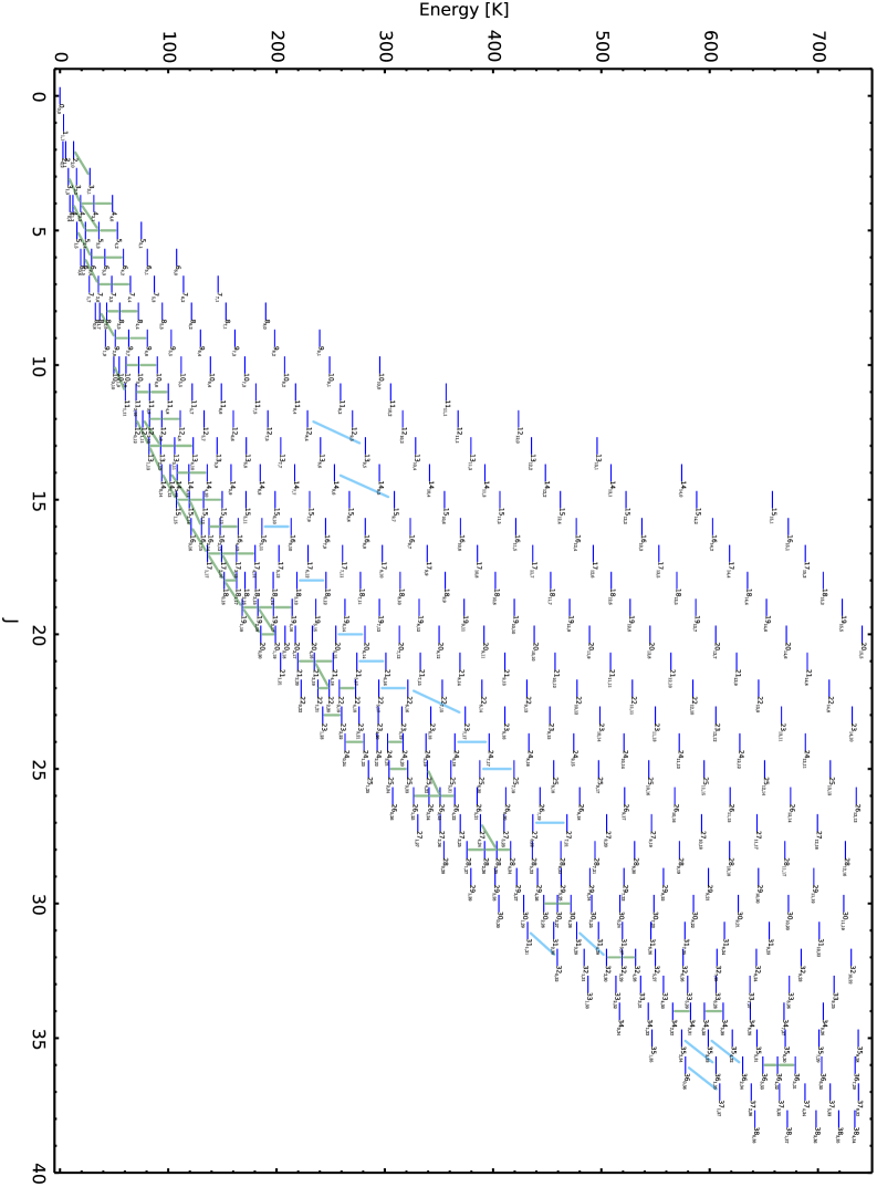
Figure 2: $\mathrm{SO}_{2}$ energy level diagram. Levels are labelled $J_{K_{a},K_{c}}$. Transitions detected with HIFI and APEX towards R Dor are indicated in light blue and green, respectively.

3.2 R Dor

Our modelling is based on the radiative transfer results obtained by Maercker et al. (in prep) for CO in R Dor. They find a mass-loss rate of $\dot{M}=1.6\times 10^{-7}\leavevmode\nobreak\ \;\mathrm{M}_{\odot}\leavevmode\nobreak\ \mathrm{yr}^{-1}$ and an expansion velocity of $\upsilon_{\infty}=5.7\leavevmode\nobreak\ \mathrm{km\,s}^{-1}$. They also find an expansion velocity profile following

$$\upsilon(r)=\upsilon_{\mathrm{min}}+(\upsilon_{\infty}-\upsilon_{\mathrm{min}})\left(1-\frac{R_{\mathrm{in}}}{r}\right)^{\beta}$$ (5)

where $\upsilon_{\mathrm{min}}=3\leavevmode\nobreak\ \mathrm{km\,s}^{-1}$ is taken to be the sound speed at $R_{\mathrm{in}}=1.6\times 10^{14}$ cm, the dust condensation radius. $\beta=1.5$ governs the acceleration of the gas, having the most significant impact in the inner regions, and hence on the excitation of the higher-energy lines. The other relevant stellar properties of R Dor are listed in Table 7.

Table 7: Stellar properties and input from CO models.

	IK Tau	R Dor	TX Cam	W Hya	R Cas
$L_{*}$ [L⊙]	7700	6500	8600	5400	8700
$D$ [pc]	265	59	380	78	176
$\upsilon_{\mathrm{LSR}}$ [$\mathrm{km\,s}^{-1}$]	34	7	11.4	40.5	25
$T_{*}$ [K]	2100	2400	2400	2500	3000
$R_{\mathrm{in}}$ [$10^{14}$ cm]	2.0	1.9	2.2	2.0	2.2
$\tau_{10}$	1.0	0.03	0.4	0.07	0.09
$\dot{M}$ [$10^{-7}\;\mathrm{M}_{\odot}\leavevmode\nobreak\ \mathrm{yr}^{-1}$]	$50$	$1.6$	40	$1$	$8$
$\upsilon_{\infty}$ [$\mathrm{km\,s}^{-1}$]	17.5	5.7	17.5	7.5	10.5
$\beta$	1.5	1.5	2.0	5.0	2.5

3.2.1 SO results

To model the 17 SO lines detected towards R Dor with APEX and HIFI, we set up a grid sampling different SO abundances and $e$-folding radii. We then ran a finer grid with steps of $0.1\times 10^{-6}$ in abundance and $0.1\times 10^{15}$ cm in $e$-folding radius to find the best possible fit to the observations. The results of our $\chi^{2}$ analysis can be seen in Fig. 3. Our resulting best-fit model, with $\chi^{2}_{\mathrm{red}}=0.90$, has a peak SO abundance relative to $\mathrm{H}_{2}$ of $(6.7\pm 0.9)\times 10^{-6}$ and $e$-folding radius $R_{e}=(1.4\pm 0.2)\times 10^{15}$ cm and is plotted against the observed lines with respect to the LSR velocity in Fig. 4. A plot illustrating the goodness-of-fit for all the lines is given in Fig. 5. The abundance profile for SO is plotted in Fig. 8 along with $\mathrm{SO}_{2}$ and the CO and $\mathrm{H}_{2}$O results from Maercker et al. (in prep.) for comparison.

One of the detected SO lines, ($8_{9}\to 7_{8}$), overlaps with $\mathrm{SO}_{2}$($16_{4,12}\to 16_{3,13}$) in its wing. We note that this is the only SO line which is significantly over-predicted by the model. Our code is unable to properly take heteromolecular overlaps such as this into account. We suspect that although the $\mathrm{SO}_{2}$ line is much fainter than the SO line (in fact it is difficult to see even in Fig. 20 where the $\mathrm{SO}_{2}$ model is overplotted), their interaction likely affects the flux from SO($8_{9}\to 7_{8}$).

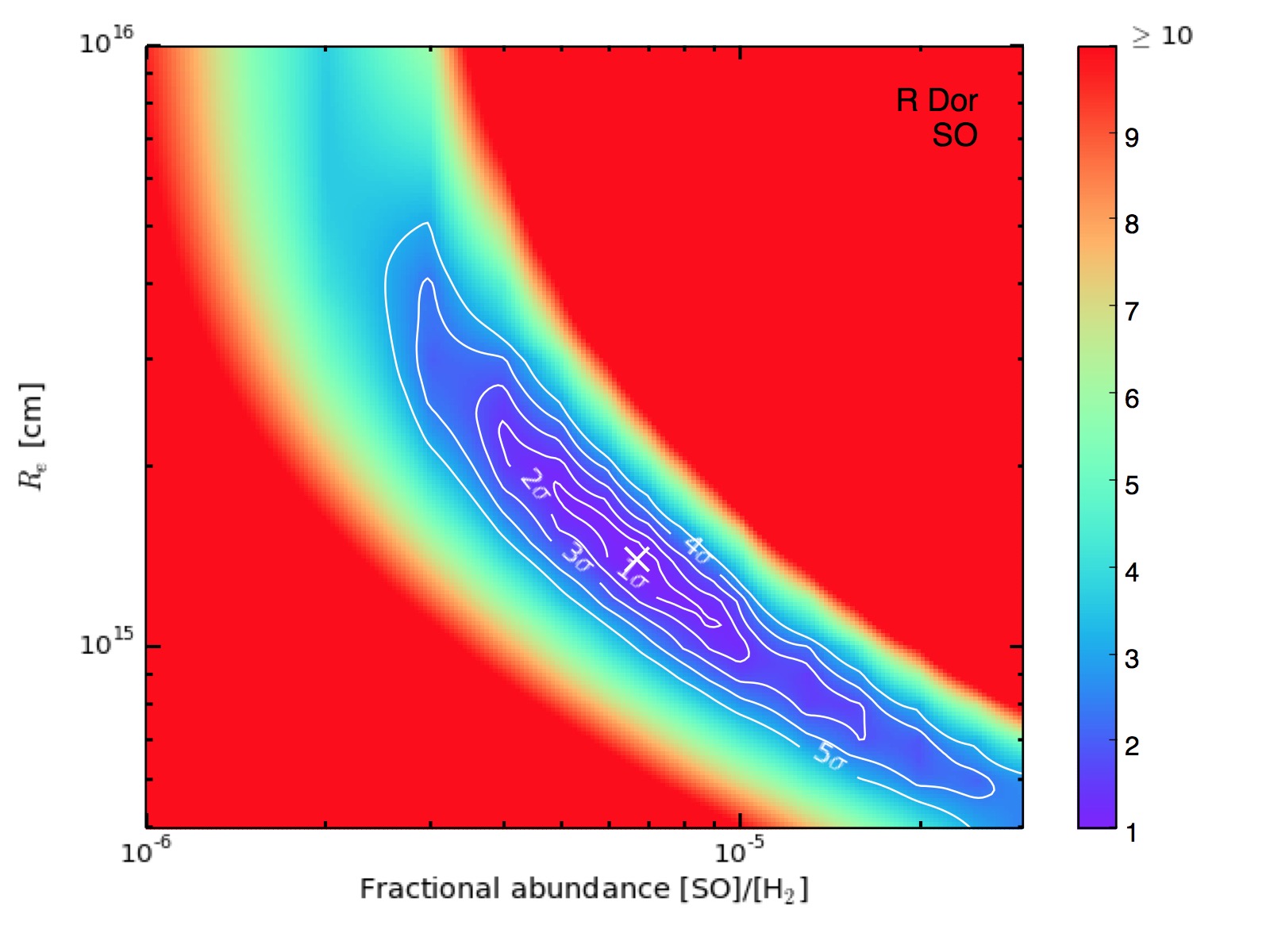
Figure 3: SO $\chi^{2}$ plots for R Dor, W Hya, IK Tau and R Cas. The contours show the confidence intervals and the shading represents the $\chi^{2}_{\mathrm{red}}$ value for the corresponding model, with the colour-bar indicating multiples of the minimum $\chi^{2}_{\mathrm{red}}$ value. The white cross indicates our best-fit model (see Table 9). For IK Tau, the slice for which $R_{w}=1.8R_{p}$ is shown. For R Cas, the slice for which $R_{w}=1.0R_{p}$ is shown.

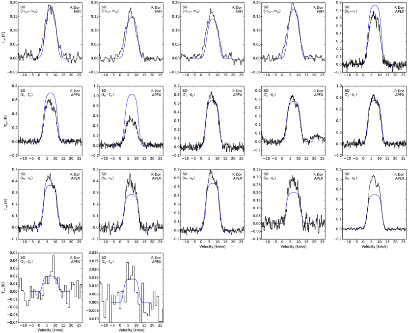
Figure 4: SO models (blue lines) and observations (black histograms) for R Dor.

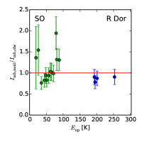
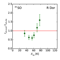
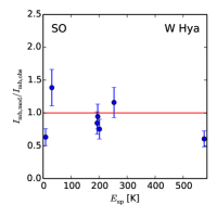
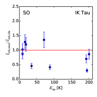
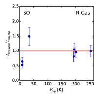
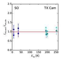
Figure 5: SO goodness of fit plots for R Dor, R Cas, IK Tau, and W Hya. New HIFI lines as well as archival data listed in Table 6 are included. The green points in the R Dor plots represent the observations from the APEX spectral survey. Undetected HIFI lines are shown as cyan points with arrows, in this case representing lower limits because the vertical axis is the ratio of model integrated intensities to observed integrated intensities or the upper limits thereof.

3.2.2 SO₂ results

We detected 100 $\mathrm{SO}_{2}$ lines in R Dor with APEX and HIFI. We exclude the $v_{2}=1$ ($25_{4,22}\to 26_{1,25}$) line at 279.497 GHz from our analysis since it is most likely a maser. We also concluded that it was not computationally viable to model the line with the highest energy level in the ground state, ($40_{4,36}\to 40_{3,37}$) at 341.403 GHz, as the number of additional levels and transitions required to fully account for this line represented a significant increase in computation time. (We would have required 3583 levels and 19889 radiative transitions.) The two excluded lines are plotted in Fig. 6.

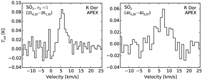
Figure 6: $\mathrm{SO}_{2}$ lines excluded from modelling for R Dor. See text for full explanation.

This leaves us with 98 detected $\mathrm{SO}_{2}$ lines with which to constrain our model. Our best fit model has $f_{p}=5.0\times 10^{-6}$, $R_{e}=1.6\times 10^{15}$ cm and $\chi^{2}_{\mathrm{red}}=3.7$. Due to the significant computational time in running $\mathrm{SO}_{2}$ models, we are unable to provide a comprehensive error analysis as we do for the SO model, hence the lack of formal uncertainties on our results. The model lines are plotted with the observed lines in Fig. 20 with goodness of fit shown in Fig. 7. Overlaps are discussed in detail in Sect. 3.2.3. Fig. 8 shows our best-fit abundance profiles for $\mathrm{SO}_{2}$ and SO, along with the results for CO and $\mathrm{H}_{2}$O from Maercker et al. (in prep.).

There is a lot of scatter in the goodness-of-fit plots in Fig. 7. There is no trend in goodness-of-fit with upper energy level or $J$, but the observed lines that are most strongly under-predicted by the model are those lines for which the upper energy level has quantum number $K_{a}\geq 6$ (see lower right plot in Fig. 7). This corresponds to the lines further away from the “backbone” of $K_{a}=0,1$ energy levels in the energy level diagram in Fig. 2. We suspect this could be partially due to our exclusion of overlaps for lines outside of the observed frequency range (see Sect. 3.1.2). When testing models with and without overlaps enabled, we note that some lines that do not participate in overlaps can still be strongly affected by the inclusion (or not) of overlaps in our model. For example $\mathrm{SO}_{2}$($27_{7,21}\to 27_{6,22}$) at 657.885 GHz was one such line, with the model predicting weaker emission by a factor of a few when overlaps were omitted. Unfortunately, due to computational limitations, it is not feasible to properly include overlaps in a full radiative transfer analysis, as discussed in Sect. 3.1.2. It should also be noted that the R Dor data were taken over a long observational campaign (see Sect. 2), so any variability in $\mathrm{SO}_{2}$ line brightnesses with pulsation period may contribute to the scatter.

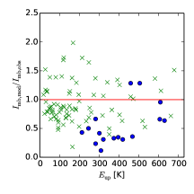
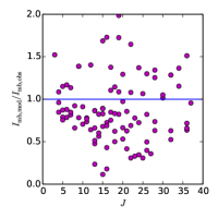
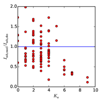
Figure 7: $\mathrm{SO}_{2}$ goodness of fit plots for R Dor. Top: Goodness of fit with upper energy level of the transition. HIFI lines are shown as blue points and APEX lines are shown as green crosses. Error bars are excluded to make the plot clearer to read. Lower left: Goodness of fit with $J$. Lower right: Goodness of fit with $K_{a}$, a clear downwards trend for $K_{a}\geq 6$.

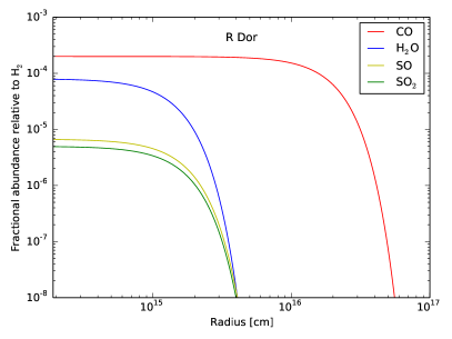
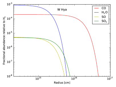
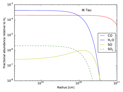
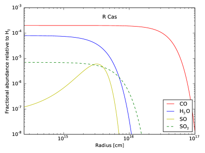
Figure 8: Abundance profiles for R Dor, W Hya, IK Tau and R Cas. The abundances for CO and $\mathrm{H}_{2}$O are taken from Maercker et al., (in prep), except for W Hya, for which they are taken from Khouri et al. (2014a, b). The dashed line for the $\mathrm{SO}_{2}$ results for IK Tau and R Cas indicates that they are tentative.

3.2.3 Overlapping lines

Table 8: Overlapping lines in R Dor

Primary line	Frequency	Secondary line	Frequency	Notes
$\mathrm{SO}_{2}$ $32_{0,32}\to 31_{1,31}$	571.553	$\mathrm{SO}_{2}$ $32_{2,30}\to 31_{3,29}$	571.532	Two distinct peaks
$\mathrm{SO}_{2}$ $13_{1,13}\to 12_{0,12}$	251.200	$\mathrm{SO}_{2}$ $8_{3,5}\to 8_{2,6}$	251.211	Two distinct peaks
SO $8_{9}\to 7_{8}$	346.528	$\mathrm{SO}_{2}$ $16_{4,12}\to 16_{3,13}$	346.524	SO line strongly dominates, $\mathrm{SO}_{2}$ line in SO wing
$\mathrm{SO}_{2}$ $24_{7,17}\to 26_{6,18}$	659.898	$\mathrm{SO}_{2}$ $40_{1,39}\to 40_{0,40}$	659.886	Primary line dominates, secondary appears in wing*
$\mathrm{SO}_{2}$ $6_{3,3}\to 6_{2,4}$	254.281	$\mathrm{SO}_{2}$ $24_{2,22}\to 24_{1,23}$	254.283	Unresolved overlap of two lines of similar strength
$\mathrm{SO}_{2}$ $32_{3,29}\to 32_{2,30}$	300.273	$\mathrm{SO}_{2}$ $24_{8,16}\to 25_{7,19}$ ($\nu_{2}=1$)	300.280	Secondary line not detected
$\mathrm{SO}_{2}$ $15_{4,12}\to 15_{3,13}$	357.241	$\mathrm{SO}_{2}$ $37_{4,34}\to 38_{1,37}$ ($\nu_{2}=1$)	357.230	Secondary line not detected
$\mathrm{SO}_{2}$ $12_{3,9}\to 12_{2,10}$	237.069	$\mathrm{SO}_{2}$ $26_{3,23}\to 25_{4,22}$ ($\nu_{2}=1$)	237.062	Secondary line not detected
$\mathrm{SO}_{2}$ $7_{3,5}\to 7_{2,6}$	257.100	$\mathrm{SO}_{2}$ $8_{3,5}\to 8_{2,6}$ ($\nu_{2}=1$)	257.099	Lines coincide very closely; not distinguishable
$\mathrm{SO}_{2}$ $13_{2,12}\to 12_{1,11}$	345.339	H13CN $4\to 3$	345.340	Lines not distinguishable in profile

.

Table 8 contains an inventory of known line overlaps for the presented lines. In our radiative transfer modelling, we are able to take into account overlaps which occur between two lines of the same molecule — i.e. two $\mathrm{SO}_{2}$ lines. (For computational purposes we only include $\mathrm{SO}_{2}$ overlaps in the range 200 GHz – 1.2 THz. Note, however, that all possible homomolecular overlaps are taken into account for SO in all modelled stars.) However, if there is a line overlap between two lines generated by different molecules, we are unable to properly treat this, as our code only allows for the modelling of one molecular species at a time. In R Dor we observe two such heteromolecular overlaps. The first between the SO($8_{9}\to 7_{8}$) and $\mathrm{SO}_{2}$($16_{4,12}\to 16_{3,13}$) lines, where the much weaker $\mathrm{SO}_{2}$ line appears in the wing of the bright SO line, and the second between $\mathrm{SO}_{2}$($13_{2,12}\to 12_{1,11}$) and H¹³CN($4\to 3$), where the two lines coincide very closely so as to be indistinguishable. Based on our model, we expect approximately half the flux to be due to the H¹³CN($4\to 3$) transition, which would agree with the H¹³CN($3\to 2$) line also covered by the APEX survey. However, without modelling H¹³CN, it is not possible to fully gauge the impact of this overlap on our model.

The remaining line overlaps for lines modelled in this paper are homomolecular.

Three of the line pairs that are treated as overlapping in the code consist of a bright primary line in the vibrational ground state and a very weak secondary line in the $\nu_{2}=1$ vibrationally excited state. As can be seen in Fig. 20, these secondary lines are not detectable above the noise in our observations, but are taken into account in our modelling.

The $\mathrm{SO}_{2}$ ($24_{7,17}\to 26_{6,18}$) line at 659.898 GHz overlaps with the $\mathrm{SO}_{2}$ ($40_{1,39}\to 40_{0,40}$) at 659.886 GHz and we would expect the latter to have an effect on the former. However, the $\mathrm{SO}_{2}$ ($40_{1,39}\to 40_{0,40}$) line falls outside of the range of energy levels we included in our model. As noted in Sect. 3.1.2, it was not feasible to include a larger number of higher energy levels, hence this particular overlap is not taken into account in our modelling.

3.2.4 Isotopologue results

Based on the analysis of 6 ³⁴SO lines, and assuming the same $e$-folding radius as found for ³²SO, we find a ³⁴SO abundance of $(3.1\pm 0.8)\times 10^{-7}$ in a best fit model that has $\chi^{2}_{\mathrm{red}}=1.4$. This gives a ³²SO/³⁴SO ratio of $21.6\pm 8.5$. The best fit model is shown in Fig. 9. The goodness of fit plot showing the ratio between the model and observed integrated intensities is shown in Fig. 5.

Modelling ³⁴$\mathrm{SO}_{2}$ in the same detailed manner as we have modelled ³²$\mathrm{SO}_{2}$ is impractical given the computational time required, the complexity of the molecular data file, and the low number of detected lines. However, all of the ³²$\mathrm{SO}_{2}$ lines we modelled are optically thin, so we can approximate the ³²$\mathrm{SO}_{2}$/³⁴$\mathrm{SO}_{2}$ ratio by comparing the intensity ratios of two lines of the same transition. The best ³⁴$\mathrm{SO}_{2}$ transition for this purpose is $20_{0,20}\to 19_{1,19}$. Comparing the integrated intensities for this transition, we find a ³²$\mathrm{SO}_{2}$/³⁴$\mathrm{SO}_{2}$ ratio of $21.6\pm 12.1$, in good agreement with the result from ³⁴SO modelling.

The solar system value of ³²S/³⁴S is 22.5 (Cameron, 1973) and Kahane et al. (1988) found a value of 20.2 for the carbon star CW Leo using SiS isotopologues, both in agreement with our results.

While a detailed model of ³⁴$\mathrm{SO}_{2}$ would be extremely time consuming, a detailed model of SO¹⁸O would not be computationally feasible. Due to the asymmetry of the two oxygen atoms, SO¹⁸O has approximately double the number of energy levels and transitions as $\mathrm{SO}_{2}$, when looking at the same energy range, meaning that an SO¹⁸O molecular data file would have to be approximately twice the size of our already very large $\mathrm{SO}_{2}$ file to probe a similar range of energies. The more complex energy level structure also means it is not possible to directly compare lines between SO¹⁸O and $\mathrm{SO}_{2}$, even when the transitions have the same quantum numbers. For ³⁴$\mathrm{SO}_{2}$ and SO¹⁸O we present the (tentative) detections in Fig. 21.

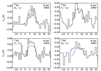
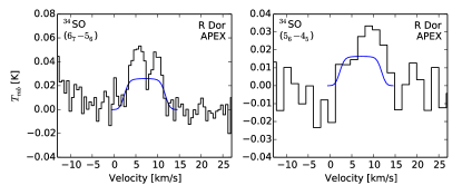
Figure 9: ³⁴SO model (blue lines) and observations (black histograms) for R Dor.

3.3 Other M stars

We model SO and $\mathrm{SO}_{2}$ line emission for the remaining stars using HIFI observations, as listed in Table 5, and archival observations with different ground-based instruments, as listed in Table 6. Several of these older observations probe energy levels significantly lower than the HIFI observations, allowing us to better constrain the size of the emitting molecular envelope. This is particularly important for IK Tau, where only the three $N=13\to 12$ SO lines were detected with HIFI, as these are emitted from a similar region of the CSE.

The stellar parameters used in our SO and $\mathrm{SO}_{2}$ models, taken from CO model results, are listed in Table 7.

3.3.1 W Hya

In the case of W Hya we find an SO model that fits the data well using the Gaussian abundance distribution given in Eq. 3. We found $f_{p}=(5.0\pm 1.0)\times 10^{-6}$ and $R_{e}=(1.5\pm 0.5)\times 10^{15}$ cm, with $\chi^{2}_{\mathrm{red}}=2.57$. This result is qualitatively similar to that of R Dor. As with R Dor, this suggests that SO in the CSE of W Hya is formed close to the star and is not found in a shell around the star as might be expected if it were a photodissociation product of another molecule such as $\mathrm{H}_{2}$S. The HIFI observations and model line plots for SO are shown in Figure 10. The corresponding $\chi^{2}$ plot is shown in Fig. 3.

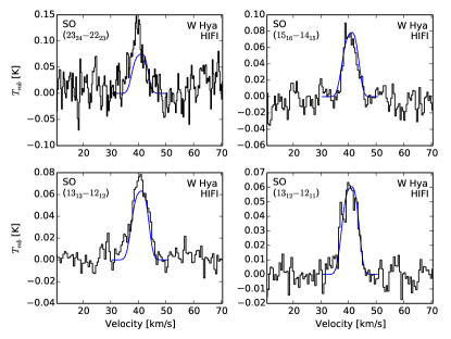
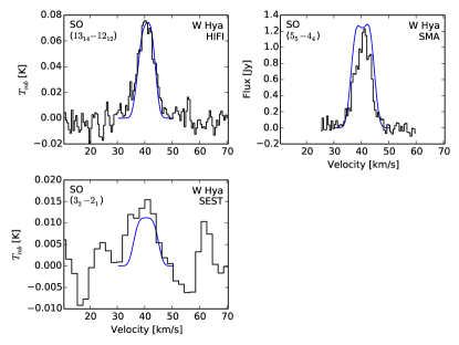
Figure 10: Models (blue lines) and observations (black histograms) for SO towards W Hya.

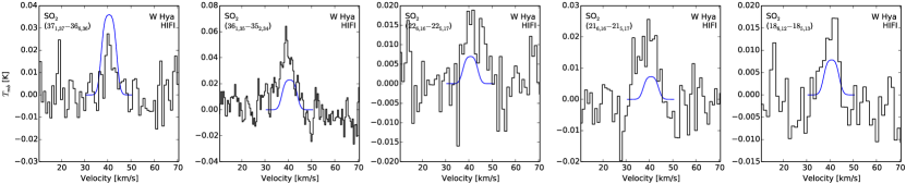
Figure 11: Models (blue lines) and observations (black histograms) for $\mathrm{SO}_{2}$ towards W Hya.

The HIFI observations and model line plots for $\mathrm{SO}_{2}$ towards W Hya are shown in Figure 11. The main difficulty we had in fitting an $\mathrm{SO}_{2}$ model was finding a model which fit the two highest-energy lines. As can be seen in Table 5, the $\mathrm{SO}_{2}$($37_{1,37}\to 36_{0,36}$) and $\mathrm{SO}_{2}$($36_{1,35}\to 35_{2,34}$) lines are only $\sim 3$ K apart in upper energy level. Also we note that the lower-energy line is almost a factor of 3 brighter than the higher-energy line. Our model invariably predicts a smaller difference in intensity with the higher-energy line being the brighter. The same is true for R Dor, however, in R Dor the detected lines reflect this (although the model fit is not perfect). This phenomenon is probably due in part to the noise in our observations but could also reflect a problem with our molecular description of $\mathrm{SO}_{2}$. In this case, the most likely cause is the cut-off in included energy levels at $J=38$. The variation in these lines cannot be due to variations in brightness due to stellar pulsations as both lines were observed simultaneously (and, indeed, all the $\mathrm{SO}_{2}$ lines in W Hya were observed within two days). In any case, the apparently outlying line of ($37_{1,37}\to 36_{0,36}$) strongly contributes to the poorly fitting model we find for $\mathrm{SO}_{2}$ in W Hya. We are able to find a better fit by excluding this line, but do not have a strong basis for doing so, hence we leave it in.

Our best fit model for $\mathrm{SO}_{2}$ has $f_{p}=5.0\times 10^{-6}$, based on a small grid with steps of $0.5\times 10^{-6}$, and $R_{e}=3.0\times 10^{15}$ cm, based on a small grid with steps of $0.5\times 10^{15}$ cm. This model has $\chi^{2}_{\mathrm{red}}=5.7$. We also test an $\mathrm{SO}_{2}$ model using the parameters we found for SO. That model is not a significantly worse fit with almost the same $\chi^{2}_{\mathrm{red}}$.

The abundance distributions for SO and $\mathrm{SO}_{2}$, along with the CO and $\mathrm{H}_{2}$O abundance distributions from Khouri et al. (2014a, b) for comparison, are shown in Fig. 8.

3.3.2 IK Tau

When we try to fit the SO IK Tau observations with a centrally peaked Gaussian distribution, we cannot constrain the $e$-folding radius with the available data. The $\chi^{2}$ analyses of centrally-peaked Gaussian models point towards very large $e$-folding radii, significantly larger (by more than half an order of magnitude) than the half-abundance radius Maercker et al. (in prep.) found for the corresponding CO envelope. Since it is highly unlikely that the SO envelope is more extensive than that of CO, we conclude that a centrally-peaked Gaussian distribution is unlikely for SO in IK Tau. Instead, we run a three-parameter grid across $f_{p}$, $R_{p}$, and $R_{w}$ (see Eq. 4) to find the best model. We find $f_{p}=(1.0\pm 0.2)\times 10^{-6}$, $R_{p}=(1.3\pm 0.2)\times 10^{16}$ cm, and $R_{w}=1.8R_{p}$ (which we gridded in steps of $0.2R_{p}$), with $\chi^{2}_{\mathrm{red}}=4.67$ and the resultant lines are shown in Fig. 12.

The $\chi^{2}$ plot for SO in IK Tau is shown in Fig. 3. IK Tau has a significantly larger $\chi^{2}$ value for the best fit model (compared with R Dor and W Hya) because of some noisy observations. This is also seen in the goodness of fit plot in Fig. 5. In comparison, R Dor and W Hya have brighter and more uniform line observations, making it easier to find a good model fit.

Decin et al. (2010a) perform a radiative transfer analysis of IK Tau in a way that is similar to our method. They find an SO abundance distribution that is similar to our shell-like distribution, but with an increased abundance in the inner region. They find an abundance at $200R_{*}$ (which corresponds to about $3\times 10^{15}$ cm) of $\sim 2\times 10^{-7}$ using two lines to fit the model. This did not change significantly in the follow up in Decin et al. (2010b) which included one of the HIFI lines as well. Our model results give a corresponding abundance about a factor of 2 higher at the same radius but using a different shape for the abundance distribution. We also use 10 lines with a broader range of energy levels to constrain the model.

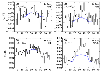
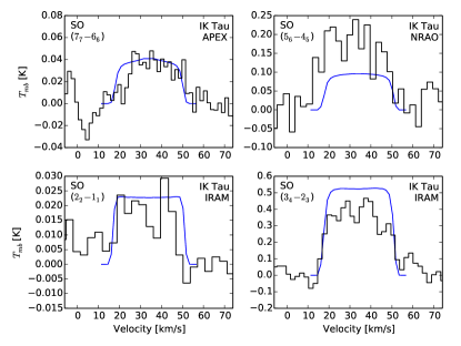
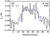
Figure 12: SO models (blue lines) and observations (black histograms) for IK Tau.

In the case of $\mathrm{SO}_{2}$ in IK Tau we are unable to include overlaps as we do for R Dor and W Hya due to the larger expansion velocity of the circumstellar gas around IK Tau. The larger expansion velocity means there are a larger number of overlaps (since the lines are about three times wider than for R Dor) which quickly become computationally infeasible to fully account for.

We could not find a consistent model for IK Tau that matched all the available observed $\mathrm{SO}_{2}$ lines. In particular, there was a very large scatter in goodness-of-fit for the lines with upper energy levels of 136 K or less (which is all of the lines other than the one HIFI observation). There was no way to simultaneously fit all these observed lines well. A centrally-peaked Gaussian model matches the data reasonably well — particularly the HIFI line, which according to the best shell model should have been a non-detection — and much better than the shell model. A Gaussian model with $e$-folding radius located at the peak of the SO distribution is a better fit than a model with the SO distribution parameters, but we find that decreasing the $e$-folding radius to $R_{e}=1\times 10^{16}$ cm gives a better fit again. We cannot constrain the $e$-folding radius better than by a factor of $\sim 2$, however, because of the large scatter in the lower-energy lines. The model we present in this paper, plotted in Fig. 13, has a peak $\mathrm{SO}_{2}$ abundance $f_{p}=2\times 10^{-6}$, and $R_{e}=1\times 10^{16}$ cm. This model has $\chi^{2}_{\mathrm{red}}=18.4$, the high value reflecting the poor overall fit.The large scatter in the IK Tau $\mathrm{SO}_{2}$ lines could be due to variability in line brightness with pulsation period. The data we used were observed at different times corresponding to different phases of pulsation. For example, the brightest lines, $(17_{1,17}\to 16_{0,16})$ and $(13_{2,12}\to 12_{1,11})$, were observed less than two weeks apart close to maximum brightness in 2006. The most under-predicted line, $(14_{3,11}\to 14_{2,12})$, was observed four months later when the star was approaching minimum brightness. On the other hand, the most well-fit lines — those with $J=5,4,3$ as can be seen in Fig. 13 — were variously taken close to minimum and maximum brightness, so perhaps it is the higher $J$ lines which are most strongly affected. Future monitoring of these lines observationally would allow us to confirm whether the effect on the higher-$J$ lines is really due to variability over a pulsation period.

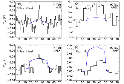
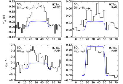
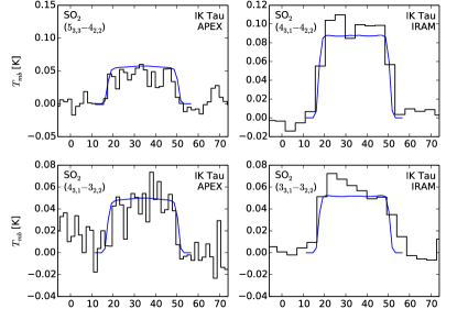
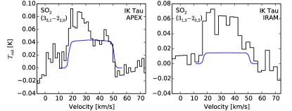
Figure 13: $\mathrm{SO}_{2}$ model (blue line) and observations (black histograms) of IK Tau. For details on the archival observations, see Table 6.

The abundance distributions for SO and $\mathrm{SO}_{2}$ in IK Tau, along with the CO and $\mathrm{H}_{2}$O abundance distributions from Maercker et al. (in prep.) for comparison, are shown in Fig. 8. In general, we do not consider our $\mathrm{SO}_{2}$ results for IK Tau conclusive. A more rigorous model which is properly able to take overlaps into consideration and which perhaps includes more lines in the intermediate to high energy range (with upper energy level $>136$ K) is recommended.

Decin et al. (2010a) have similar issues modelling the $\mathrm{SO}_{2}$ in IK Tau, especially with the ($17_{1,17}\to 16_{0,16}$) and ($13_{2,12}\to 12_{1,11}$) lines which we also strongly under-predict, as can be seen in Fig. 13. When they exclude these two lines, Decin et al. (2010a) find a high inner abundance of $\mathrm{SO}_{2}$, in general agreement with our results. The poor fit of our model could be a result of unusual structure in the CSE of IK Tau or could be a result of not being able to properly consider overlaps in the $\mathrm{SO}_{2}$ model. The higher wind velocity would also lead to more overlapping lines overall — including in regions we have not observed — which could have an effect on the overall energy distribution between all molecular energy levels.

Kim et al. (2010) use a combination of Monte-Carlo radiative transfer modelling, to find CSE properties, and LTE formulations, to determine SO and $\mathrm{SO}_{2}$ abundance for IK Tau. For SO they find fractional abundances in the range 3 to $8\times 10^{-7}$ and for $\mathrm{SO}_{2}$ their fractional abundances were in the range $4\times 10^{-6}$ to $1\times 10^{-5}$. Their results are not accompanied by clear abundance distributions, making them difficult to compare with our results. Nevertheless, their SO result is very close to our peak abundance for SO, while their $\mathrm{SO}_{2}$ result is much higher than we found.

3.3.3 R Cas

As with IK Tau, we find that a model with a centrally peaked Gaussian distribution of SO does not match the observed data. We again run a three-parameter grid to find the best shell-model fit to the data and find $f_{p}=(6.0\pm 1.2)\times 10^{-6}$, $R_{p}=(3.2\pm 0.3)\times 10^{15}$ cm, and $R_{w}=1.0R_{p}$ cm (gridded in steps of $0.2R_{p}$), with $\chi^{2}_{\mathrm{red}}=3.12$. The resultant model lines are shown in Fig. 14 with the observations. The $\chi^{2}$ plot for SO in R Cas is shown in Fig. 3 and the goodness of fit plot is included in Fig. 5.

As there are only 2 $\mathrm{SO}_{2}$ lines observed towards R Cas, we are only able to find an approximate model for $\mathrm{SO}_{2}$. As with IK Tau, a shell-like model based on the R Cas SO results does not fit the $\mathrm{SO}_{2}$ observations. Our best model has $f_{p}=7\times 10^{-6}$ (best within steps of $1\times 10^{-6}$) and $R_{e}=6\times 10^{15}$ cm (best within steps of $1\times 10^{15}$ cm). In Fig. 15 we plot the HIFI detection with our model. An abundance plot for SO, $\mathrm{SO}_{2}$, CO and $\mathrm{H}_{2}$O towards R Cas is shown in Fig. 8.

We note that the HIFI detection in Fig. 15 has a central narrow peak, much narrower than the gas expansion velocity, This skews the overall integrated line intensity somewhat. Interestingly, IK Tau has a similar narrow peak in the same transition line (see Fig. 13), also at approximately the stellar velocity. R Dor does not have such a peak and W Hya may have one which is significantly less bright with respect to the rest of the emission line. The cause of this feature is unclear.

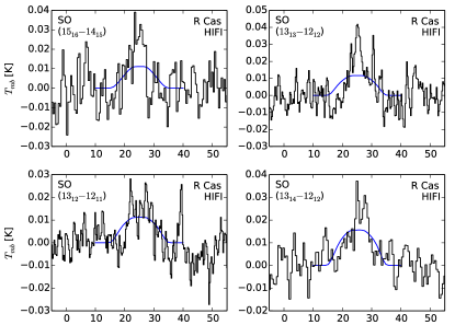
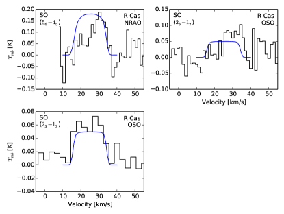
Figure 14: SO models (blue lines) and observations (black histograms) for R Cas.

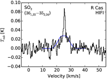
Figure 15: $\mathrm{SO}_{2}$ model (blue line) and observation (black histogram) for R Cas.

3.3.4 TX Cam

In the case of SO towards TX Cam, we do not have sufficient constraints to run a full grid and perform a $\chi^{2}$ analysis as we did for the other stars. Instead we aim to fit the archival lines and find the largest $R_{w}$ allowed by the HIFI non-detections. The best model with these assumptions has $f_{p}=1.7\times 10^{-6}$, $R_{p}=1.4\times 10^{16}$ cm and $R_{w}=1.6R_{p}$. We plot the detected lines with our model in Fig. 16. The goodness of fit, represented by the ratio between model integrated intensities and observed integrated intensities, is plotted in Fig. 5. We stress that the dearth of observational results leaves our model poorly constrained and this is just one possible model that fits the available data. We can, however, rule out a centrally peaked model, as in that case we would expect the HIFI lines to have been detected, given the constraints on the fit from the archival lines.

There were no $\mathrm{SO}_{2}$ lines detected towards TX Cam.

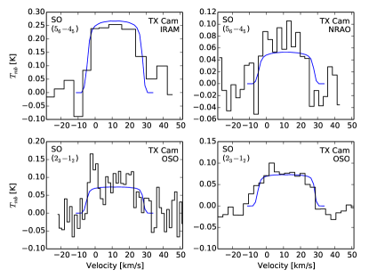
Figure 16: SO models (blue lines) and observations (black histograms) for TX Cam. We only plot the archival SO detections, not the non-detections from HIFI.

Table 9: SO and $\mathrm{SO}_{2}$ model results

	IK Tau	R Dor	TX Cam	W Hya	R Cas
$f_{p,\mathrm{SO}}$ $\times 10^{-6}$	$1.0\pm 0.2$	$6.7\pm 0.9$	1.7*	$5.0\pm 1.0$	$6.0\pm 1.2$
$R_{e,\mathrm{SO}}$ [$\times 10^{15}$ cm]	-	$1.4\pm 0.2$	-	$1.5\pm 0.5$	-
$R_{p,\mathrm{SO}}$ [$\times 10^{15}$ cm]	$13\pm 2$	-	14*	-	$3.2\pm 0.3$
$R_{w,\mathrm{SO}}$ [$\times R_{p,\mathrm{SO}}$]	1.8	-	1.6*	-	1.0
$\chi^{2}_{\mathrm{red}}$ (SO)	4.7	0.9	-	2.6	3.1
$N_{\mathrm{SO}}$	10	17	4 (4)	7	7
$f_{p,\mathrm{SO}_{2}}$ $\times 10^{-6}$	0.86	5.0	-	5.0	7
$R_{e,\mathrm{SO}_{2}}$ [$\times 10^{15}$cm]	10	1.6	-	3.0	6
$\chi^{2}_{\mathrm{red}}$ ($\mathrm{SO}_{2}$)	14.3	3.7	-	5.7	-
$N_{\mathrm{SO}_{2}}$	14	98	0	5	2

4 Discussion

4.1 SO distribution

Our results for circumstellar SO are summarised in Table 9. In Fig. 17 we plot the circumstellar SO abundance profiles of the stars we modelled. We also show the radial range probed by the available observational data for each line with a thicker line. These ranges were found by considering the brightness distributions for each emission line and the radii at which these fall to half of their maximum values. It is interesting to note that for R Cas, IK Tau, and TX Cam, the three stars with shell-like SO distributions, the location of the peak is found progressively further out with increasing mass-loss rate. The two low mass-loss rate stars, however, both seem to have centrally peaked SO distributions, which could be interpreted as shells with peaks close to the star, especially if the peaks are near or within our inner radii. Looking at the three stars with shell-like SO distributions, there also seems to be a trend of decreasing SO abundance with increasing mass-loss rate (or with the radius of peak SO abundance).

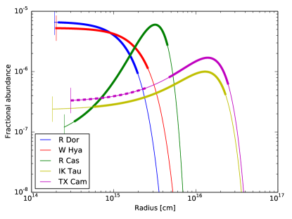
Figure 17: SO abundance distributions for all stars modelled. The vertical lines represent the dust condensation radii, where our models stop. The thicker sections of the curves represent the area probed by our observations and for TX Cam the thick dashed line is the area probed by the upper limits imposed by the HIFI non-detections.

In Fig. 18 we plot the peak positions against the wind density, ${\dot{M}}/{\upsilon_{\infty}}$, and fit a power law to the three higher mass-loss rate stars (R Cas, TX Cam and IK Tau). The results for these stars are well fit by a power law

$$R_{p}\propto\left(\frac{\dot{M}}{\upsilon_{\infty}}\right)^{\alpha_{R}}$$ (6)

with $\alpha_{R}=1.15\pm 0.24$. We extend the power law to predict the peak positions for R Dor and W Hya, were they also to fit this trend. This predicts the peak in SO abundance for R Dor to lie at $1.0\times 10^{15}$ cm, which is close to the $R_{e}$ we found, and for W Hya the predicted SO peak lies at $4.4\times 10^{14}$ cm, about three times smaller than the $e$-folding radius. Running models with shell-like distributions at the predicted peaks, we found they could not provide as good a fit for either R Dor or W Hya as the star-centred Gaussian models. In general, the best shell models had at least twice the $\chi^{2}$ values of the best star-centred Gaussian models. Given the region probed by our observations as shown in Fig. 17, it is not surprising that changing the inner abundance would have an effect on the model fit.

We performed a similar fit for the peak abundance values against density for the three highest mass-loss rate stars. The results for these stars are well fit by a power law

$$f_{p}\propto\left(\frac{\dot{M}}{\upsilon_{\infty}}\right)^{\alpha_{f}}$$ (7)

with $\alpha_{f}=-1.29\pm 0.17$, Fig. 18. Doing a similar extrapolation to predict the peak abundance values for R Dor and W Hya based on the power law, we find fractional abundance predictions of $2.2\times 10^{-5}$ for R Dor and $5.8\times 10^{-5}$ for W Hya. Both of these are higher than the values we find from our modelling and in the case of W Hya this represents more sulphur than should be available, i.e. it exceeds the solar and ISM abundances (see below). Because the SO abundance cannot increase with decreased mass-loss rate indefinitely, there must be a maximum SO abundance set by the abundance of sulphur.

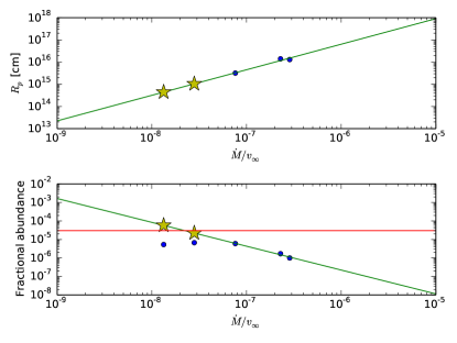
Figure 18: Trends in SO peak radius (top) and fractional abundance (bottom) against the circumstellar density measure, $\dot{M}/\upsilon_{\infty}$. The green lines are the trends fitted to the three higher mass-loss rate stars (R Cas, TX Cam and IK Tau), while the yellow stars are the predicted locations of the lower mass-loss rate stars (R Dor and W Hya) based on the trend. In the fractional abundance plot, the red line shows the hard limit for SO abundance based on solar S abundance and the blue points in line with the yellow stars represent the real abundance values for R Dor and W Hya.

The shell-like distributions of SO for the three stars with the highest mass-loss rates means that circumstellar chemistry, most likely related to photodissociation, must play an important role, in these cases. It is therefore interesting to compare with results on photodissociation for other species. H₂O is particularly interesting here, since, as will be discussed below, SO (and also SO₂) may owe its origin to the presence of circumstellar OH, which in turn is a photodissociation product of H₂O. Netzer & Knapp (1987) predict a peak OH radius that scales with both mass-loss rate and expansion velocity. Their formulation has been used by Maercker et al. (2008, 2009); Schöier et al. (2011); Danilovich et al. (2014) and others to define the $e$-folding radius of $\mathrm{H}_{2}$O, since OH is a photodissociation product of $\mathrm{H}_{2}$O and peaks in abundance where $\mathrm{H}_{2}$O drops off. In Fig. 19 we plot our SO peak abundance radii or $e$-folding radii (as relevant) against the $\mathrm{H}_{2}$O $e$-folding radii of the same stars found by Maercker et al. (in prep.) and Khouri et al. (2014b, for W Hya). We find a strong correlation, which is close to being 1:1. The chemistry of SO will be discussed in Sect. 4.3.

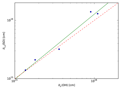
Figure 19: The peak abundance radii of SO (for R Cas, TX Cam, and IK Tau) and the $e$-folding radii of SO (for R Dor and W Hya), plotted against the $e$-folding radii of $\mathrm{H}_{2}$O found by Maercker et al (in prep.) and Khouri et al. (2014b, for W Hya). The solid green line is the best fit to the data and the dashed red line traces a 1:1 relationship.

4.2 SO₂ distribution

Our results for circumstellar SO₂ are summarised in Table 9. For R Dor and W Hya we find circumstellar $\mathrm{SO}_{2}$ distributions of similar size and abundance to the circumstellar SO distributions. Our results for the higher mass-loss rate stars, however, are less clear. For both IK Tau and R Cas, the best models are centrally-peaked Gaussian distributions of $\mathrm{SO}_{2}$, rather than the shell-like models we found for SO. For IK Tau, we were unable to constrain the $e$-folding radius better than by a factor of 2 and for R Cas we only had two observations, but in both cases shell models similar to the corresponding SO models are ruled out. Our $\mathrm{SO}_{2}$ results for IK Tau and R Cas suggest that $\mathrm{SO}_{2}$ is formed in the inner regions irrespective of the mass-loss rate. It appears that $\mathrm{SO}_{2}$ is formed more favourably than SO in the inner regions. There does not appear to be a strong correlation between $e$-folding radius and mass-loss rates or $\mathrm{H}_{2}$O $e$-folding radii, as we found for SO, but this might become clearer if we add more $\mathrm{SO}_{2}$ observations to our models, especially for R Cas and W Hya. We emphasise that our SO₂ results for the higher mass-loss rate stars, R Cas and IK Tau, are particularly uncertain.

4.3 Comparisons with chemical models

There exist two studies of the abundances of SO and SO₂ in the extended atmospheres of AGB stars (Cherchneff, 2006; Gobrecht et al., 2016). In both cases the effects of shock-induced chemistry, due to pulsational motion, are included. Cherchneff (2006) has chosen TX Cam as the representative star, and the modelling covers the region from 1 to 5 stellar radii, $R_{*}$, which means that the outer reach of their model is approximately an order of magnitude smaller than our inner radii. For their model star with C/O = 0.75, they find an SO abundance at $5R_{*}$ of $3\times 10^{-7}$, and an SO₂ abundance several orders of magnitude lower than this. Gobrecht et al. (2016) use IK Tau as the example, and extend the calculations to 10 stellar radii (the outer radius of their model then approximately meets the inner radius used by us). Their model focuses on the shock chemistry in this region, much of which varies with the pulsation phase. Their abundances of SO and $\mathrm{SO}_{2}$ are much lower than we observe, at $\sim 10^{-8}$ and $\sim 2\times 10^{-9}$, respectively. This means that the predicted SO and $\mathrm{SO}_{2}$ abundances close to the star, at least for these higher mass-loss rate stars, are substantially lower than we derive for our sample stars.

The shell-like SO distributions for the higher mass-loss rate stars suggest a circumstellar origin. Willacy & Millar (1997) describe circumstellar chemical models of four M-type AGB stars, including R Dor, TX Cam, and IK Tau. Their models differ from ours in terms of CSE parameters, for example taking the inner radius to be $2\times 10^{15}$ cm, about an order of magnitude larger than our inner radii. They assume that all the sulphur is carried by H₂S that is eventually photodissociated. SO is subsequently formed through the following reactions

$$\mathrm{S}+\mathrm{OH}\to\mathrm{SO}+\mathrm{H}$$ (8)

$$\mathrm{SH}+\mathrm{O}\to\mathrm{SO}+\mathrm{H}$$ (9)

which are favoured depending on the availability of OH and SH, respectively, and with Eq. 8 dominating at the lower gas temperatures in the CSE. Following this, SO can be destroyed through

$$\mathrm{SO}+\mathrm{OH}\longleftrightarrow\mathrm{SO}_{2}+\mathrm{H}$$ (10)

and hence form SO₂. Unfortunately, they only visualise their model results for TX Cam, the least well-constrained star of our sample. Nevertheless, the location of the peak of the SO distribution that we find for TX Cam agrees quite well with their predicted peak location. Our peak abundance is about 50% higher than theirs, but this must be considered to be within the errors. Their $\mathrm{SO}_{2}$ distribution for TX Cam peaks at roughly the same radius as SO, but with a peak abundance about an order of magnitude lower than that of SO (as we do not have any $\mathrm{SO}_{2}$ detections for TX Cam, we cannot compare this directly). The molecular column densities they list for R Dor, IK Tau, and TX Cam are, in general, a few orders of magnitude lower than those predicted by our models.

In conclusion, our SO results for the outer CSE are reasonably consistent with the results of Willacy & Millar (1997) for the higher mass-loss rate objects, although they do not predict a peak abundance that decreases with mass-loss rate. Thus, an origin through OH is likely, a result that is further strengthened by the correlation between SO and H₂O sizes that we found. However, we note that neither Cherchneff (2006) nor Gobrecht et al. (2016) predict high abundances of H₂S in the upper atmosphere. For the lower mass-loss rate objects, where the SO abundance is high close to the star, the models of Cherchneff (2006) and Gobrecht et al. (2016) fail by more than two orders of magnitude to reproduce our estimated abundances. They even fail to reproduce the inner SO abundances for the higher mass-loss rate stars.

In the case of SO₂ we find no evidence for a photo-induced circumstellar origin along the Willacy & Millar (1997) model for any of our objects. Once again, we caution that the results for R Cas and IK Tau are uncertain. The SO₂ abundances that we estimate for R Dor and W Hya are an order of magnitude higher than those predicted by Cherchneff (2006) and Gobrecht et al. (2016).

4.4 Sulphur chemistry: can we account for all the sulphur?

AGB stars and their progenitors do not produce S via nucleosynthesis. As such, the quantity of sulphur available to form molecules in the CSE of an AGB star is fixed and not dependent on the stage of evolution or mass of the star in question. Rudolph et al. (2006) find an S/H ratio in the ISM of $\sim 10^{-5}$ in the solar neighbourhood and Lodders (2003) indicate a solar S/H abundance of $1.5\times 10^{-5}$. All stars in our sample are at distances $<\,400$ pc and hence can be assumed to trace a similar S/H abundance. In this work we refer to the fractional molecular abundance with respect to $\mathrm{H}_{2}$. Hence, assuming all hydrogen is in the form of $\mathrm{H}_{2}$ in the CSE, we will take the S/$\mathrm{H}_{2}$ ratio to be $\sim 2$ to $3\times 10^{-5}$, which represents the maximum total amount of sulphur that should be found in an AGB star.

For R Dor and W Hya we find combined SO and $\mathrm{SO}_{2}$ abundances of $\sim 1.2\times 10^{-5}$ and $\sim 1.0\times 10^{-5}$, respectively. Hence, in these cases most of the sulphur is locked up in SO and $\mathrm{SO}_{2}$ within the inner regions of the CSE and within the errors. This result is consistent with the non-detections (or low-level emission) for CS and SiS in the APEX spectral scan of R Dor, and no reported detections of these species towards W Hya. In the case of R Cas, the combined SO and $\mathrm{SO}_{2}$ abundances in the mid-CSE is $\sim 1.4\times 10^{-5}$, suggesting that these two species carry all the sulphur, but here the uncertainty on the $\mathrm{SO}_{2}$ abundance is substantial. For the high mass-loss rate object IK Tau, the combined SO and $\mathrm{SO}_{2}$ abundance is well below that of sulphur.

In general, higher mass-loss rate stars also show definitive detections of other S-bearing molecules. For example, SiS was detected in several carbon and M-type stars by Schöier et al. (2007) and Danilovich et al. (2015). Schöier et al. (2007) reported circumstellar SiS abundances of $4\times 10^{-7}$, $4\times 10^{-7}$, and $1\times 10^{-7}$ for R Cas, TX Cam, and IK Tau, respectively, suggesting that SiS is less abundant than SO and $\mathrm{SO}_{2}$ by up to an order of magnitude, at least in the outer CSE. It should be noted that Schöier et al. (2007) assume a Gaussian distribution of SiS centred on the star, but find their model fit greatly improved when they include a high-abundance inner component, which could represent the SiS reservoir before depletion through dust condensation. Decin et al. (2010a), who model IK Tau in detail, also find evidence of depletion of SiS.

Another S-bearing molecule, CS, has mainly been detected in carbon stars rather than M-type stars. CS has been detected and modelled in IK Tau by Kim et al. (2010) and Decin et al. (2010a), detected in TX Cam and IK Tau by Bujarrabal et al. (1994, with non-detections in R Cas and W Hya) and Lindqvist et al. (1988, with a non-detection in R Cas). Derived CS abundances for M-type stars have generally been low, in the range $\sim 10^{-8}$ to $\sim 5\times 10^{-8}$ (see Bujarrabal et al., 1994; Decin et al., 2010a, for examples).

$\mathrm{H}_{2}$S is considered as a parent species of sulphur in the chemical modelling of Willacy & Millar (1997). However, $\mathrm{H}_{2}$S has not been widely detected in AGB stars other than in OH/IR stars. For example, in the HIFISTARS project $\mathrm{H}_{2}$S was only detected in AFGL 5379 (Justtanont et al., 2012), despite being in the observed range for all stars except TX Cam, while Justtanont et al. (2015) detected $\mathrm{H}_{2}$S in all OH/IR stars observed with SPIRE and some observed with PACS. In a study of 25 stars, Ukita & Morris (1983) detected $\mathrm{H}_{2}$S only in OH231.8+4.2 aka the Rotten Egg Nebula. Omont et al. (1993) detected $\mathrm{H}_{2}$S in several high mass-loss rate stars, including several OH/IR stars. Of the stars we modelled, Ukita & Morris (1983) did not detect $\mathrm{H}_{2}$S in W Hya, R Cas, and TX Cam, but it was detected in IK Tau by Omont et al. (1993) and De Beck et al. (in prep.). This suggests that $\mathrm{H}_{2}$S may require high densities to form, or may be able to survive longer in the CSEs of high mass-loss rate stars, or that the excitation conditions are such that the emission is only bright enough in the very high mass-loss rate stars to be detectable. We note that Gobrecht et al. (2016) predict a fairly rapid decline of $\mathrm{H}_{2}$S inside of the dust condensation radius (which is where our models start) even for IK Tau, which is a relatively high mass-loss rate object.

To check what the lack of detections predicts in terms of $\mathrm{H}_{2}$S abundances, we run radiative transfer models for R Dor and IK Tau to find upper limits for the $\mathrm{H}_{2}$S abundances based on the non-detections in HIFI, the non-detection in APEX for R Dor, and the SMA detection in IK Tau by De Beck et al. (in prep.). We used the ortho-$\mathrm{H}_{2}$S molecular data file available on LAMDA (Schöier et al., 2005) which includes the lowest 45 rotational energy levels, 139 radiative transitions with frequencies taken from JPL and 990 collisional transitions taken from Dubernet et al. (2009) for temperatures from 5–1500 K. For IK Tau, using the detection from De Beck et al. (in prep.) and the HIFI upper limit to also constrain the envelope size, we find a small envelope with $R_{e}\simeq 4\times 10^{14}$ cm and $f_{p}\simeq 4\times 10^{-6}$. This is consistent with a rapid destruction of $\mathrm{H}_{2}$S. For R Dor, using both non-detections and assuming the $R_{e}$ we find for SO, we find an upper limit on the abundance of $f_{p}\lesssim 2.5\times 10^{-7}$. If we instead use the $\mathrm{H}_{2}$S envelope size found for IK Tau, the abundance upper limit increases slightly to $f_{p}\lesssim 6\times 10^{-7}$. In any case, these results limit the possibility that $\mathrm{H}_{2}$S is a significant S-carrier in the inner CSE, certainly for the low mass-loss rate objects.

None of the molecules discussed thus far have been found in sufficient quantities towards higher mass-loss rate AGB stars to account for the full amount of expected sulphur. It is possible that the remaining sulphur is locked up in dust or left as atomic S or locked up in molecules that are difficult to detect for various reasons, such as the spectral region they are most likely to emit in, as is the case with HS. Both Cherchneff (2006) and Willacy & Millar (1997) predict a rapid decline of HS with radius as it is consumed by various chemical processes (although we note that the two studies make predictions for different regions around the star). The only detection of HS in the literature is through ro-vibrational lines identified by Yamamura et al. (2000) towards R And (an S-type AGB star). They estimate a molecular abundance of HS/H $\sim 1\times 10^{-7}$, which is well below the sulphur limit. There have been no other detections of circumstellar HS, although it has been detected in the ISM (see e.g. Neufeld et al., 2015).

To fully study the issue of sulphur in the CSEs of AGB stars of different mass-loss rates, a more thorough investigation including more molecular species — such as SiS, CS, and $\mathrm{H}_{2}$S in addition to SO and $\mathrm{SO}_{2}$ — across a larger sample of stars is needed.

5 Conclusions

We present new APEX observations of a very large number of SO and $\mathrm{SO}_{2}$ lines towards the low mass-loss rate M-type AGB star R Dor. Combining these data with higher-frequency observations from Herschel/HIFI, we compute comprehensive radiative transfer models to determine the molecular abundances and distributions of the two molecules. For R Dor we find a Gaussian abundance distribution centred on the star, with a peak SO fractional abundance of $(6.7\pm 0.9)\times 10^{-6}$ and $e$-folding radius of $(1.4\pm 0.2)\times 10^{15}$ cm, and an $\mathrm{SO}_{2}$ fractional abundance of $5.0\times 10^{-6}$ and $e$-folding radius of $1.6\times 10^{15}$ cm. Our ³⁴SO model assumes the same $e$-folding radius as for ³²SO and we find an abundance of $(3.1\pm 0.8)\times 10^{-7}$. This gives an ³²SO/³⁴SO ratio of $21.6\pm 8.5$, which is in agreement with previous results from other nearby stars.

We also model SO in four other M-type AGB stars that were observed as part of HIFISTARS: IK Tau, TX Cam, W Hya, and R Cas. For TX Cam for we are only able to provide an upper limit model since there are no SO lines detected with HIFI. Of these four stars only W Hya has a similar SO distribution to R Dor. The other three stars, all of which have higher mass-loss rates, are best fit with shell-like abundance distributions. We find that the radial position of the peak of the distributions increases with mass-loss rate, while the peak abundances decrease. The location of the peaks of the SO distributions correlates with the photodissociation of $\mathrm{H}_{2}$O into OH (itself partly dependent on mass-loss rate), suggesting that the production of SO depends on the availability of OH to participate in the formation process.

We are only able to model $\mathrm{SO}_{2}$ in an additional three stars, IK Tau, W Hya, and R Cas, owing to the dearth of detections towards TX Cam. For W Hya we find an $\mathrm{SO}_{2}$ distribution similar to SO in abundance and envelope size. We have some difficulty fitting an $\mathrm{SO}_{2}$ model to observations for IK Tau and ultimately find an uncertain model which differs in shape from the SO distribution. For R Cas the $\mathrm{SO}_{2}$ model is also very uncertain because there are only two detected lines.

Overall, the circumstellar SO and $\mathrm{SO}_{2}$ abundances are much higher than predicted by chemical models of the extended stellar atmosphere. These two species may also account for all the available sulphur in the lower mass-loss rate stars. The S-bearing parent molecule appears not to be $\mathrm{H}_{2}$S. The $\mathrm{SO}_{2}$ models for the higher mass-loss rate stars are less conclusive, but suggest an origin close to the star for this species. This is not consistent with present chemical models. The combined circumstellar SO and $\mathrm{SO}_{2}$ abundances are significantly lower than that of sulphur for these higher mass-loss rate objects.

To better constrain the behaviour of sulphur we need more observations of SO and $\mathrm{SO}_{2}$, as well as other S-bearing species. Observations of a larger sample of stars will also allow us to confirm the trends we see in the SO abundance distributions.

Appendix A R Dor plots

Our best fit model lines for $\mathrm{SO}_{2}$ in R Dor are plotted along with the corresponding observations in Fig. 20. For more details see Sect. 3.2.2.

The tentative detections of the isotopologues ³⁴$\mathrm{SO}_{2}$ and SO¹⁸O from the APEX survey towards R Dor are plotted in Fig. 21.

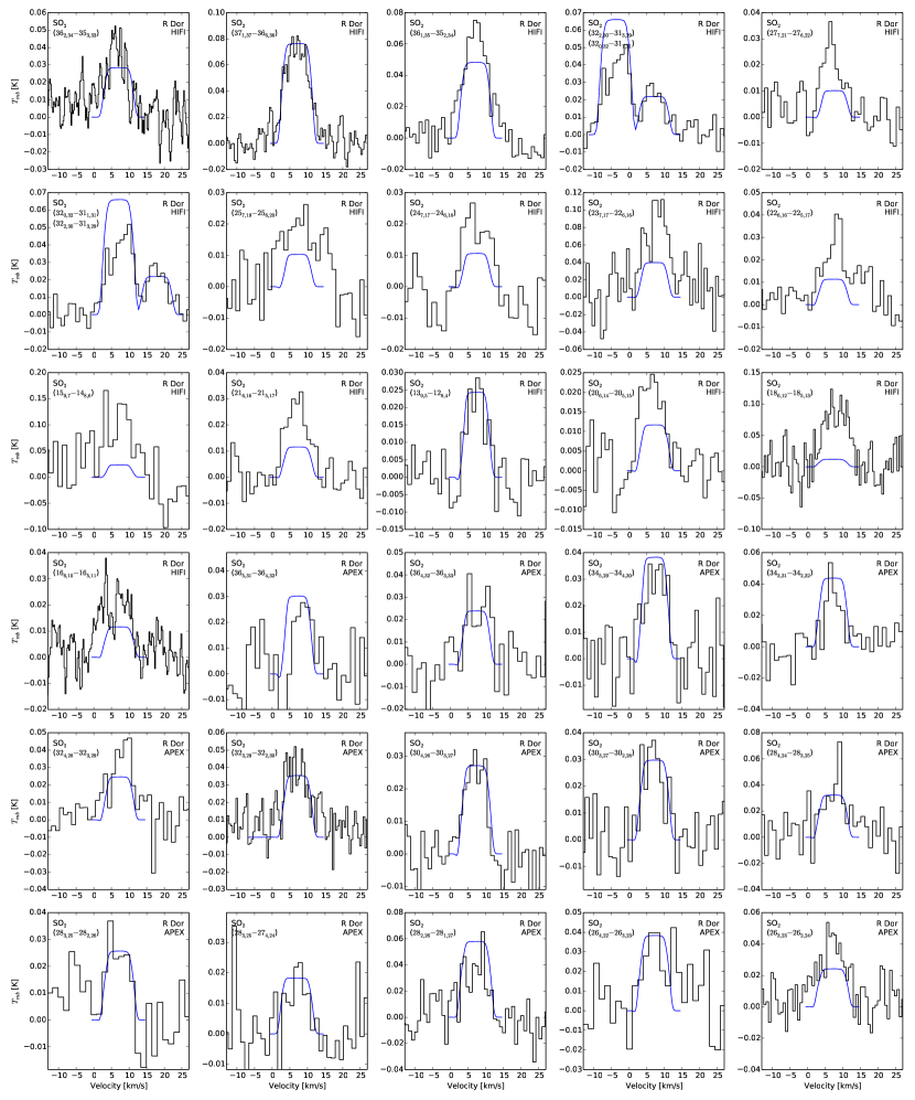
Figure 20: $\mathrm{SO}_{2}$ model (blue line) and observations (black histograms) of R Dor. In the case of overlapping lines, the top line listed is always the line centred at $\upsilon_{\mathrm{LSR}}=5.7\leavevmode\nobreak\ \mathrm{km\,s}^{-1}$.

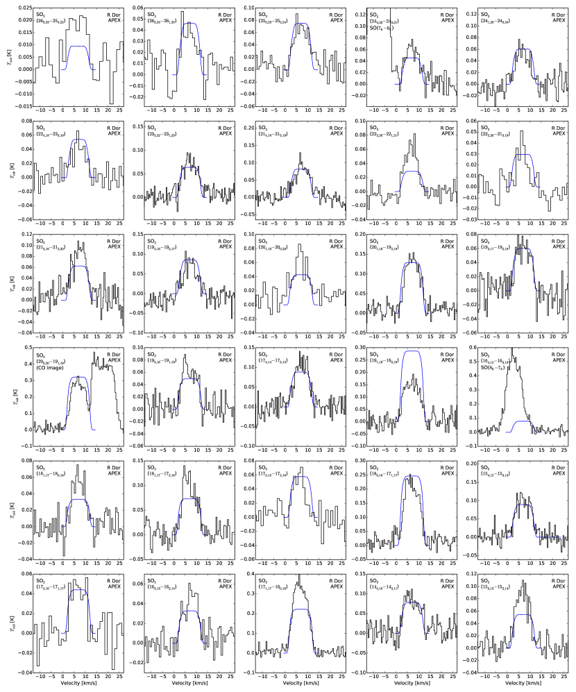
Figure 20: continued.

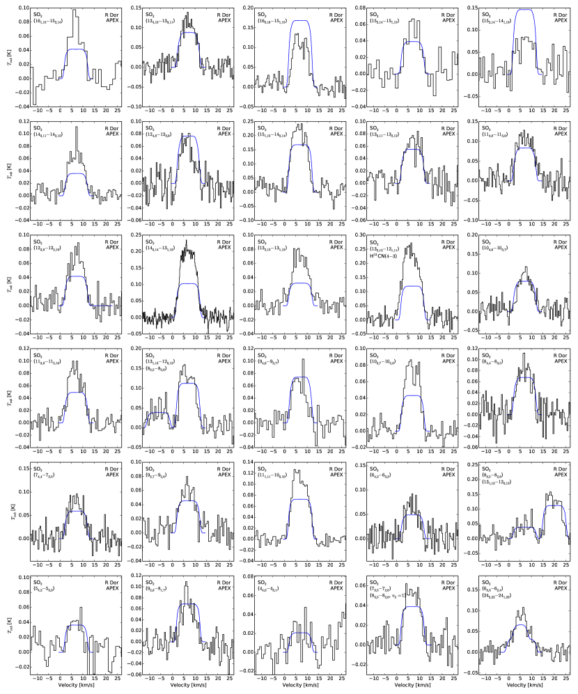
Figure 20: continued.

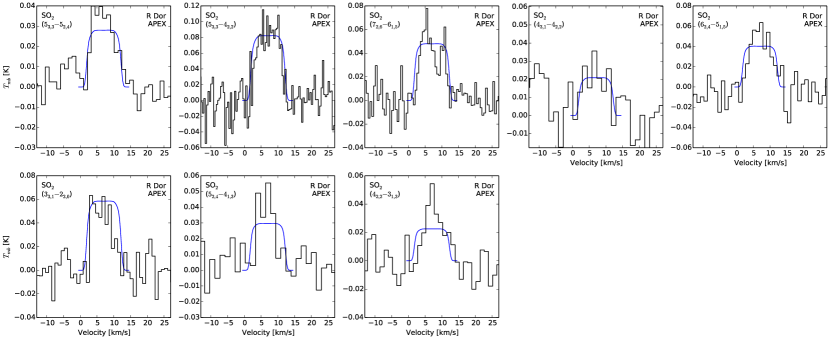
Figure 20: continued.

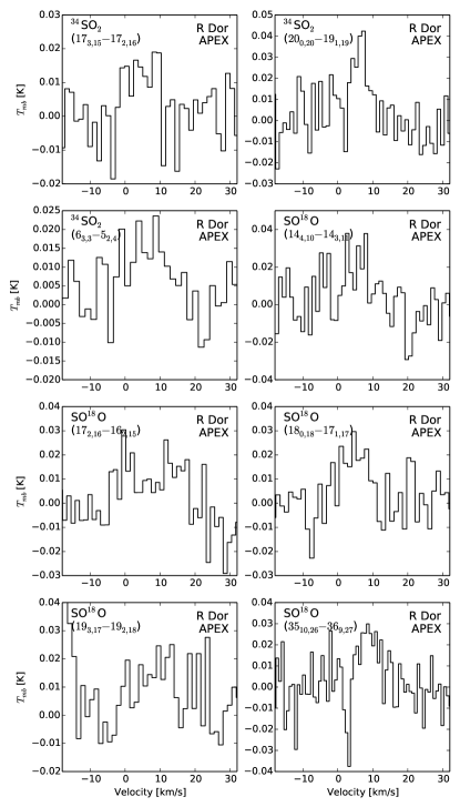
Figure 21: Detections of the isotopologues ³⁴$\mathrm{SO}_{2}$ and SO¹⁸O towards R Dor.

Appendix B HIFI OBSIDs

The observation IDs for the HIFI observations used in this work are given in Table 10, including the non-detections used to constrain our TX Cam SO model.

Table 10: HIFI OBSIDs for observations used in this work.

Star	OBSID
IK Tau	1342190198
	1342191594
R Dor	1342198355
	1342197982
	1342200969
	1342200906
TX Cam	* 1342205330 *
	* 1342205309 *
W Hya	1342200951
	1342200981
	1342200929
R Cas	1342200974
	1342198335