Classification and Ranking of Fermi LAT Gamma-ray Sources from the 3FGL Catalog using Machine Learning Techniques

Abstract

We apply a number of statistical and machine learning techniques to classify and rank gamma-ray sources from the Third $Fermi$ Large Area Telescope (LAT) Source Catalog (3FGL), according to their likelihood of falling into the two major classes of gamma-ray emitters: pulsars (PSR) or Active Galactic Nuclei (AGN). Using 1904 3FGL sources that have been identified/associated with AGN (1738) and PSR (166), we train (using 70% of our sample) and test (using 30%) our algorithms and find that the best overall accuracy ($>$96%) is obtained with the Random Forest (RF) technique, while using a logistic regression (LR) algorithm results in only marginally lower accuracy. We apply the same techniques on a sub-sample of 142 known gamma-ray pulsars to classify them into two major subcategories: young (YNG) and millisecond pulsars (MSP). Once more, the RF algorithm has the best overall accuracy ($\sim$90%), while a boosted LR analysis comes a close second. We apply our two best models (RF and LR) to the entire 3FGL catalog, providing predictions on the likely nature of unassociated sources, including the likely type of pulsar (YNG or MSP). We also use our predictions to shed light on the possible nature of some gamma-ray sources with known associations (e.g. binaries, SNR/PWN). Finally, we provide a list of plausible X-ray counterparts for some pulsar candidates, obtained using Swift, Chandra, and XMM. The results of our study will be of interest for both in-depth follow-up searches (e.g. pulsar) at various wavelengths, as well as for broader population studies.

1 Introduction

The field of gamma-ray ($>$100 MeV) astronomy has long been plagued by the double problem of low number of photons (and hence, sources), and their poor characterization. Indeed, the angular resolution of gamma-ray instruments is typically measured in degrees or arcminutes at best, also being a strong function of energy (improving with increasing energy). Thus, one of the earliest gamma-ray catalogs, the Second COS-B catalog (2CG), contained only 25 sources and 21 of them were unidentified (Swanenburg et al., 1981), while two decades later, the Third EGRET Catalog (3EG) contained 271 sources  (Hartman et al., 1999), almost two thirds of which remained unidentified, despite intense follow-up efforts (Thompson, 2008).

The Fermi Large Area Telescope (LAT), launched in 2008, represents a giant leap in capabilities compared to past instruments. With its silicon-strip detector technology, wide field of view (2.4 sr), and high duty cycle ($>$95%), the LAT has not only already detected over 1000 times more photons than EGRET did, but these cover a far broader energy range (20 MeV to $>$300 GeV) and are much better characterized (Atwood et al., 2009).

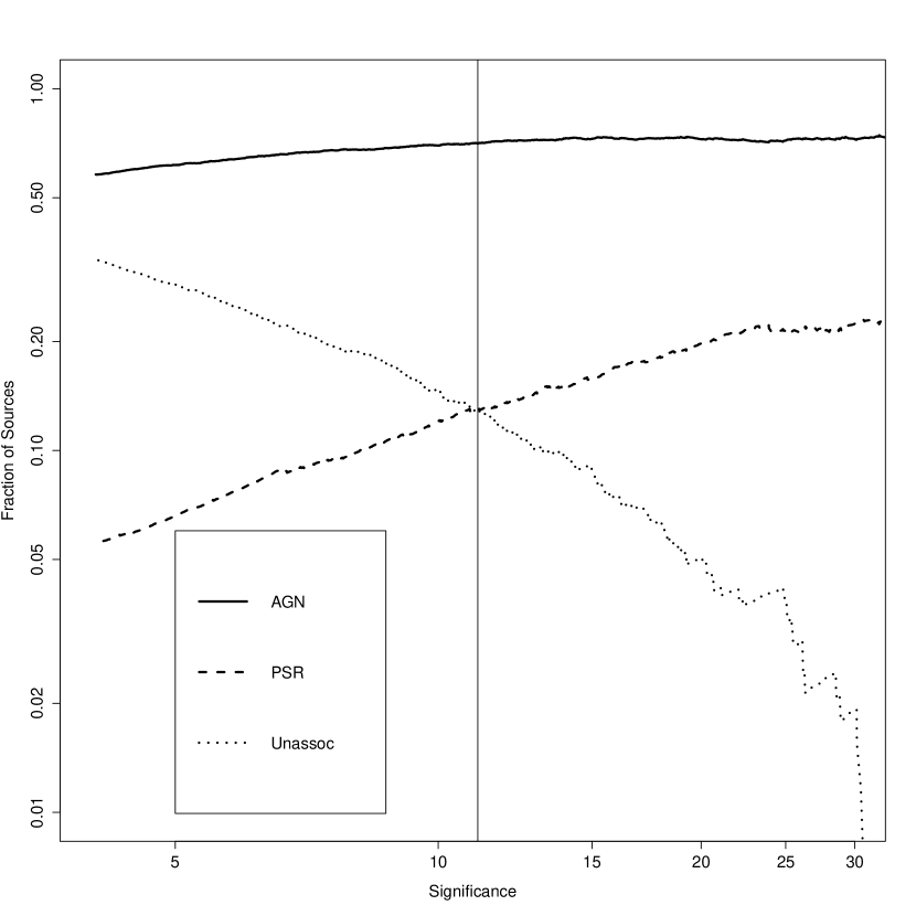
Figure 1: Fraction of 3FGL sources in the three major categories (AGN, PSR, and Unassociated) as a function of the (4-year) significance of the source. The vertical line represents the lowest significance of a pulsar found in a blind search of gamma-ray data so far (PSR J1023-5746, 11.1$\sigma$).

Within a few months of launch, the LAT team released a first list of 205 highly-significant ($>10\sigma$) sources. Known as the Bright Source List (also referred to as 0FGL (Abdo et al., 2009c)), this list represented a big improvement over previous catalogs, as illustrated by the fact that fewer than 20% of 0FGL sources were unassociated at the time of publication. Full-fledged Fermi-LAT catalogs have been released periodically since then, based on 11 months (1FGL, Abdo et al., 2010), two years (2FGL, Nolan et al., 2012), and most recently, four years of data (3FGL, Acero et al., 2015a). The number of known ($>$ 100 MeV) gamma-ray sources now stands at over 3000, with approximately one third of these in the unassociated category (Acero et al., 2015a). Figure 1 shows the fraction of 3FGL sources in the three broad categories, Active Galactic Nuclei (AGN), pulsars (PSR), and Unassociated sources as a function of the (4-year) significance of the source. The sharp drop in the fraction of gamma-ray sources that are pulsars, with decreasing significance (from $\sim 20\%$ of $>20\sigma$ sources, to $\sim 10\%$ of $\sim 10\sigma$ sources), in contrast to the fraction of AGN (a relatively uniform $\sim 60\%$) suggests that the discovery space for new (relatively gamma-bright) pulsars remains significant.

In addition to uncovering large numbers of new gamma-ray sources, the improved sensitivity of the LAT also enables a much better characterization of these sources, facilitating their identification. Among the earliest scientific results from the LAT, was the discovery of a large population of radio-quiet gamma-ray pulsars (Abdo et al., 2009b; Saz Parkinson et al., 2010), using a new blind-search technique developed specifically for the very long time series expected with the LAT (Atwood et al., 2006). These findings confirmed some predictions that many of the unidentified EGRET sources in the Galactic plane were pulsars (e.g. Yadigaroglu & Romani, 1995), favoring outer gap pulsar models (Cheng et al., 1986; Romani, 1996, 2014), where the gamma rays are generated in the outer magnetosphere, as opposed to polar cap models, where the emission comes from closer to the neutron star surface (e.g. Harding & Muslimov, 1998).

Perhaps even more surprising than the large number of young, radio-quiet pulsars discovered by the LAT was the detection of a large population of gamma-ray millisecond pulsars (MSPs) (Abdo et al., 2009a), something which, though not entirely unforeseen (e.g. Harding et al., 2005), has exceeded all expectations. Through the joint efforts of the LAT team and radio astronomers working at the major radio observatories around the world, the Fermi LAT Pulsar Search Consortium (PSC) has been carrying out extensive radio observations of both newly-discovered LAT gamma-ray pulsars, as well as carrying out new pulsar searches in LAT unassociated sources (Ray et al., 2012). This has led to the discovery of over 70 new pulsars to date (e.g. Ransom et al., 2011), the vast majority of which are MSPs.

Aside from pulsars, there are many classes of astrophysical objects that emit gamma rays. In fact, the 3FGL Catalog lists around twenty different gamma-ray source classes. By far the two largest classes are, broadly speaking, pulsars (PSR) and Active Galactic Nuclei (AGN), especially those of the blazar variety (Acero et al., 2015a). Indeed, AGN detected by the LAT can be further subdivided into many different classes (e.g. flat-spectrum radio quasars (FSRQs), BL Lacs, etc.). For extensive details, including the latest catalog of LAT-detected AGN, see Ackermann et al. (2015).

It has been known for some time now that the two main classes of gamma-ray sources (AGN and PSR) can be roughly distinguished by their timing and spectral properties: AGN display variability on month-long time scales and have energy spectra that break more softly than pulsars in the LAT energy band. Pulsars tend to be non-variable (on long time scales) and have spectra with more curvature, breaking on both ends, and therefore poorly described by a simple power law, normally requiring the addition of an exponential cut-off at a few GeV. This was illustrated graphically in the 1FGL catalog by means of a Variability-Curvature plot (See Figure 8 from Abdo et al., 2010), showing pulsars and AGN clustering in opposite corners. Indeed, a number of bright pulsar candidates were identified this way (e.g. Kong et al., 2012; Romani, 2012), and later discovered to be pulsars (Pletsch et al., 2012; Ray et al., 2014).

The large increase in the number of gamma-ray sources detected with the LAT, as well as the somewhat crude and arbitrary (as well as subjective) nature of visual inspection techniques, make it desirable to develop an automated scheme to classify candidate sources, according to their predicted source class. In recent years there has been an explosion of interest in data science, and the application of statistical techniques to all fields, including astronomy (for a nice overview of recent developments in machine learning and data mining techniques applied to astronomy, see Way et al., 2012). Various groups have started applying these techniques to astronomical data. Recently,  Masci et al. (2014) applied the Random Forest algorithm to the classification of variable stars using the Wide-field Infrared Survey Explorer (WISE) data, achieving efficiencies of up to $\sim$85%. In the gamma-ray regime, a number of groups have worked on both unsupervised learning (Lee et al., 2012) and supervised learning (Mirabal et al., 2012) techniques. Indeed, the Fermi LAT Collaboration applied two different machine-learning techniques to the automatic classification of 1FGL sources: logistic regression and classification trees. By combining the two methods, a success rate of $\sim$80% was estimated for the correct classification of the gamma-ray source class (Ackermann et al., 2012). An artificial neural network approach has also been implemented and applied to the 2FGL catalog with some promising preliminary results (Salvetti, 2013).

We have explored a large number of statistical techniques for ranking data (e.g. Alvo & Yu, 2014) and have applied some of the most commonly used algorithms to the problem of classification of LAT gamma-ray sources in the most recent 3FGL Catalog (Acero et al., 2015a). Our goal is not to firmly establish the class of each of the $\sim$1000 unassociated gamma-ray sources in 3FGL; rather, it is to provide an objective measure that quantifies the likelihood of each source of belonging to one of the two major classes (pulsar or AGN), for the purpose of aiding in the necessary follow-up studies and searches (mostly in other wavelengths) that can conclusively determine the nature of each individual source. In pointing out sources that are unlikely to belong to either of the big source classes, our study also serves to highlight gamma-ray sources that might have a more exotic origin (e.g. dark matter annihilation). Finally, our results may be useful for population studies, or to estimate the number of new gamma-ray sources in each class that we might expect to identify in the future.

The structure of the paper is as follows. In Section 2 we describe the data sets used in the paper as well as some of the key predictor parameters employed. Section 3 discusses the various algorithms we considered, with an emphasis on those that proved most successful (Random Forest and Logistic Regression). Next, in Section 4 , we discuss the application of these algorithms to the 3FGL catalog and provide an overview of our results. Finally, Section 5 provides a discussion of our key results and conclusions, including our predictions on the nature of both the unassociated sources, as well as certain gamma-ray sources with known associations (e.g. gamma-ray binaries and SNR/PWNe). We also provide a list of plausible X-ray counterparts for some of our best pulsar candidates, obtained through our follow-up program of LAT gamma-ray sources with Swift, Chandra, and XMM.

2 Data and Feature Selection

The Fermi LAT Third Source Catalog (3FGL) was publicly released through the Fermi Science Suppport Center (FSSC) in January 2015, with a few minor updates being posted around the time of official publication (Acero et al., 2015a). The results presented here make use of the uptdated version released on 2015 May 18 (FITS file gll_psc_v16.fit). The 3FGL catalog contains 3,034 gamma-ray sources, of which 1010 are unassociated.

2.1 Training and Testing Sets

Since we are interested in applying a number of supervised learning techniques to classify sources according to their likelihood of falling into two broad classes (PSR and AGN), our first step involves selecting sources from 3FGL that are known to fall into these two categories. We select all sources that are identified or associated with pulsars (i.e. sources classified as PSR or psr, respectively, in 3FGL), and all sources that are identified or associated with any type of AGN, including FSRQs, BL Lacs, etc (i.e. sources of the following class: FSRQ, fsrq, BLL, bll, BCU, bcu, RDG, rdg, NLSY1, nlsy1, agn, ssrq, and sey). After filtering out sources with missing values (six AGN and one pulsar, namely PSR J1513–5908), we are left with a total of 1904 sources, of which 1738 are AGN and 166 are PSR. We created training and testing sets by randomly selecting 70% and 30% of these sources, respectively. In summary, our training sample contains 1,217 AGN and 116 PSR, while our testing sample contains 521 AGN and 50 PSR.

Because we are also interested in the classification of pulsars into ‘young’ (YNG) and millisecond (MSP), we further split the known gamma-ray pulsars into these two sub-samples. We make use of the public list of LAT-detected gamma-ray pulsars and cross-correlate these with the 3FGL catalog, obtaining a list of 142 known gamma-ray pulsars (77 YNG and 65 MSP) which, we randomly split up into a training set containing 70% of the sample (52 YNG and 47 MSP) and a testing set with the remaining 30% (25 YNG and 18 MSP).

2.2 Feature Selection

The 3FGL Catalog contains a large number of measured parameters on each source, covering everything from the source positions and uncertainties, to fluxes in various bands, etc. In addition to all the parameters included in 3FGL, we also defined the following hardness ratios, following Ackermann et al. (2012), as:

$hr_{ij}=(EnergyFlux_{j}-EnergyFlux_{i})/(EnergyFlux_{j}+EnergyFlux_{i})$

where $i$ and $j$ are indices corresponding to the five different LAT energy bands defined in the 3FGL catalog: i=1: 100–300 MeV, i=2: 300 MeV – 1 GeV, i=3: 1–3 GeV, i=4: 3–10 GeV, and i=5: 10–100 GeV, respectively. The energy flux in each band is computed by integrating the photon flux, using the measured spectral index.

We started out with a large number (35) of potential parameters on which to train our sample. Using a two sample t-test, we then determined how the various parameters were correlated to each other (e.g. Signif_Avg is highly correlated with Flux_Density) and removed highly correlated ($\mid$$\rho$$\mid>$0.7) parameters as well as parameters related to the position of the source (e.g. GLAT, GLON). We then applied a log transformation to some parameters that displayed highly skewed distributions (e.g. Variability_Index). We dropped sources with missing values for any of our predictor parameters, leaving a total of 3021 sources, out of the original 3034. Table 1 shows the 9 predictor parameters that we ended up using in our various models for classifying PSR vs AGN, along with the range and median of these parameters in our data sets. These include the well-known curvature and variability parameters (Signif_Curve and Variability_Index, respectively), the spectral index and flux density of the source, the uncertainty in the energy flux above 100 MeV (Unc_Energy_Flux100), and the four hardness ratios constructed using the five different energy bands and equation described above (i.e. $hr_{12}$, $hr_{23}$, $hr_{34}$, and $hr_{45}$). For the MSP vs YNG classification, we added GLAT (Galactic Latitude) as a possible predictor parameter. In Appendix A.1 we provide the R script used to obtain and clean the data, as well as to perform our detailed feature selection.

3 Classification Algorithms

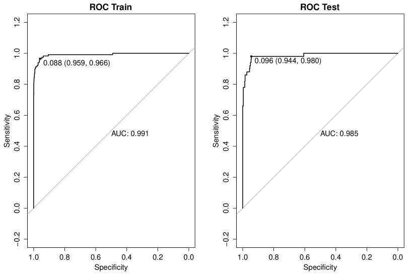
Figure 2: ROC curves for the LR model for the AGN vs PSR classification. On the left is the curve obtained on the training set, showing that the best threshold (P=0.088) results in a specificity of 0.959 and sensitivity of 0.966. The one on the right shows the corresponding values for the model applied to the testing set.

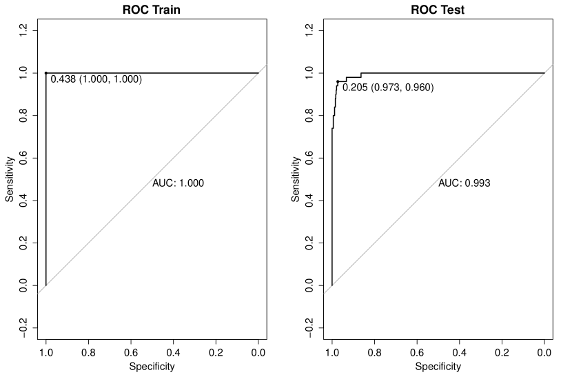
Figure 3: ROC curves for the RF model for the AGN vs PSR classification. On the left is the curve obtained on the training set, showing that the best threshold (P=0.438) results in a specificity of 1.0 and sensitivity of 1.0. The plot on the right shows that the corresponding values for the model applied to the testing set results in 0.973 and 0.960, respectively.

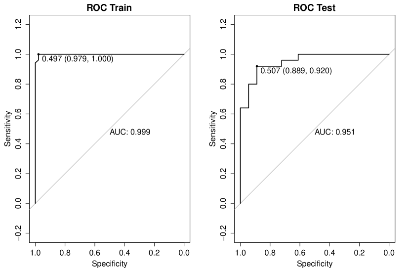
Figure 4: ROC curves for the Boosted LR model for the YNG vs MSP classification. On the left is the curve obtained on the training set, showing that the best threshold (P=0.497) results in a specificity of 0.979 and sensitivity of 1.0. The plot on the right shows that the corresponding values for the model applied to the testing set results in 0.889 and 0.920, respectively.

We considered a long list of algorithms (see Tables 2 and 3 for a complete list), including Decision Trees, Support Vector Machines (SVM), a simple logistic regression (LR) model (with both forward and backward stepwise elimination), various modified versions of LR (e.g. Boosted LR, logistic decision trees), Random Forest (RF), as well as some combination of methods (e.g. a 2-step method involving decision trees followed by LR). We used the RWeka package (Hornik et al., 2009; Witten & Frank, 2011), along with the pROC R package (Robin et al., 2011) to draw Receiver Operating Characteristic (ROC) curves, commonly used in the data mining and machine learning communities to measure the performance of a classifier. In such a curve, one plots sensitivity (true positive rate) vs specificity (true negative rate) for varying thresholds, allowing us to evaluate the tradeoffs involved in each choice, with the ultimate goal being to classify correctly the largest proportion of pulsars in our sample, while keeping the proportion of mis-classifications as low as possible. Figures 2 and 3 show the ROC curves for our two best algorithms in the AGN vs PSR classification, while Figures 4 and 5 show the corresponding ROC curves for the best two algorithms in the YNG vs MSP classification. We define the best threshold as that which maximizes the sum of both terms (sensitivity + specificity, see Appendix A.2 for the relevant R scripts). We also used the randomForest (Liaw & Wiener, 2002) R package to fit random forests and the e1071 (Meyer et al., 2014) R package to fit SVM models. Ultimately, we settled on the RF algorithm, for its overall accuracy, and LR for its slightly better sensitivity to pulsar classification. In the following sections we provide some details on the most successful models we decided to apply to the 3FGL Catalog.

3.1 Random Forest

Random forest (Breiman, 2001, hereafter RF) is an ensemble learning method which uses decision trees as building blocks for classification, regression and other tasks. By aggregating the predictions based on a large number of decision trees, RF generally improves the overall predictive performance while reducing the natural tendency of standard decision trees to over-fit the training set. RF is essentially an extension of a Bootstrap aggregating method called Tree bagging (Breiman, 1996). First of all, tree bagging for classification generates $B$ different training sets by sampling with replacement from the original training set. Then it builds a separate tree for each training set, resulting in $B$ fitted trees, and finally for each new observation, it generates the predicted class probability by taking the average of the $B$ predicted class probabilities from all $B$ fitted trees.

RF provide an improvement over bagged trees by way of a random small tweak that decorrelates the trees. Its main idea is that in each step of identifying the best split of a node in the tree growing stage, a random sample of $m$ parameters drawn from all the predictor parameters is used for consideration in selecting the best split for that node. Typically, a value of $m\sim\sqrt{p}$ is used, where $p$ is the total number of parameters tried at each split. By forcing each split to consider only a subset of the predictor parameters, the splits will not always be constructed from the strongest predictor but some other potential strong predictors, thereby making the RF more reliable. It is thus advantageous to use RF when there exists multicollinearity in the predictor parameters. The detailed algorithm can be found in the book by James et al. (2013).

In this paper, we make use of the randomForest package (Liaw & Wiener, 2002) in R. In order to ensure the stability of our results, we grew a large number of trees (10,000 vs the default of 500) and scanned over a range of values of $m$. We found that a value of $m$=2 was optimum, giving an OOB estimate of the error of 2.3%.

The randomForest package can also generate a variable importance measure for each parameter in terms of the mean decrease in accuracy (MDA), which is computed from permuting the OOB data: For each tree, the prediction error on the OOB portion of the data is recorded (error rate in the classification). Then the same is done after permuting each predictor variable. The difference between the two are then averaged over all trees (Liaw & Wiener, 2002).

The randomForest package also computes the proximity measure, which, for each pair of elements (i, j), represents the fraction of trees in which elements i and j fall in the same terminal node. This can be used to calculate the “outlyingness” of a source, as the reciprocal of the sum of squared proximities between that source and all other sources in the same class, normalized by subtracting the median and dividing by the median absolute deviation, within each class (Liaw & Wiener, 2002). Figure 6 shows the outlyingness of all 3FGL sources, with respect to the PSR and AGN classes. Note that most pulsars have large values of “AGN outlyingness”, while most AGN have large values of “PSR outlyingness”. A large value of “outlyingness” along both axes could imply a different gamma-ray source class altogether (i.e. non-Pulsar and non-AGN).

3.2 Logistic Regression

Logistic regression (hereafter LR) is a very popular probability model that was developed by Cox (1958) and Walker & Duncan (1967). The model can be used to predict a binary response based on one or more predictor parameters (features). For an 0/1 binary response variable $y$ and $p$ predictor parameters $x_{1},...,x_{p}$, the logistic regression model can be written as

$$y\mid x\sim Bernoulli(\pi)$$

and

$$logit(\pi)\equiv\log\frac{\pi}{1-\pi}=\beta_{0}+\beta_{1}x_{1}+...+\beta_{p}x_{p}$$

where $\beta=(\beta_{0},\beta_{1},...,\beta_{p})$ is a vector of unknown parameters which can be estimated by the maximum likelihood method. For further details on logistic regression, including its use as a classifier, see Hosmer et al. (2013).

Both forward and backward stepwise methods are considered in parameter selection. Forward stepwise method starts with no predictor parameters in the model, and then recursively adds parameters one at a time according to the Akaike Information Criterion (AIC). Backward stepwise method is performed similarly except that it starts with all predictor parameters in the model and proceeds by dropping parameters one at a time. In our study, we found that both methods gave the same result.

3.3 Boosted Logistic Regression

Boosted logistic regression is a powerful classifier based on additive logistic regression fitted by stage-wise optimization of the Bernoulli log-likelihood (Friedman et al., 2000). In a two-class problem, the additive logistic regression is of the form:

$$\log\frac{P(y=1\mid x)}{P(y=0\mid x)}=\sum_{m=1}^{M}f_{m}(x)$$

where $f_{m}(x)$ is learned in fitting the $m$th logistic regression on a weighted training data. Its basic idea is to adaptively change the frequency weights of the observations in the training data according to the performance of the previous logistic model. Unlike fitting a single model to the data which may not fit the data well or potentially suffer from over-fitting, the boosting approach instead, by sequentially fitting the logistic regression models, gradually improves the model fit in the regions where it originally did not perform well.

Friedman et al. (2000) developed an algorithm for fitting additive logistic regression models, named as the LogitBoost algorithm which can be implemented using the LogitBoost function in the RWeka package (Hornik et al., 2009; Witten & Frank, 2011).

3.4 Model Building Procedure

In order to determine the optimal cutoff probability value of the prediction generated from each model, we adopted a 10-fold cross-validation method. The procedure of model building is summarized as follows:

1. We partitioned our 3FGL data set at random into 70% for training and 30% for testing, as described in Section 2.1.

2. We divided the training set randomly into 10 equal-size subsets.

3. We used 9 subsets to build a model and apply the fitted model to test on the remaining subset. We then repeated this procedure for all 10 subsets until all the subsets were tested.

4. We obtain the ROC curve based on all the tested subsets and determine the best cutoff value.

5. Using the training data to build a model, we then apply the fitted model and best cutoff value to generate our prediction (“PSR" or “AGN") for the testing data.

4 Application of the algorithms to 3FGL

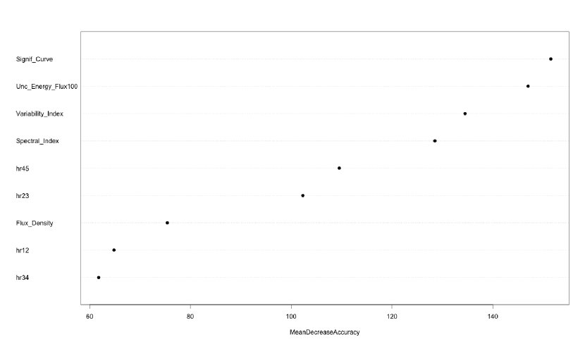
Figure 7: Mean Decrease in Accuracy for the best Random Forest model to classify sources into AGN vs Pulsar.

Figure 7 shows the relative importance of the input parameters in the RF model, expressed as the mean decrease in accuracy, as described in Section 3.1. Note that in some cases we have transformed the parameters by taking the log, due to the skewness of the distributions. We note that, perhaps not surprisingly, the curvature significance and variability parameters (Signif_Curve and Variability_Index) are two of the three most important predictor variables, while the uncertainty in the energy flux (Unc_Energy_Flux100) also turns out to be very important, perhaps as a proxy for the quality of the spectral fit of the source. In the case of the classification of pulsars into YNG and MSP, we added GLAT (Galactic Latitude), which we found to be useful in discriminating between the two classes (In fact, it is the second most important parameter, see Figure 8). Table 4, on the other hand, shows the values of the parameters ($\beta_{0},\beta_{1},...$) corresponding to the various predictor parameters in the best logistic regression model (backwards stepwise), giving also an indication of the significance of each one (Variability_Index being the most significant, in this case).

4.1 Results

After applying a large number of algorithms to the problem of gamma-ray source classification, we concluded that the RF technique provides the overall best accuracy (96.7%), while LR (with backward stepwise elimination) provides only slightly lower overall accuracy (94.7%), but a better sensitivity to pulsar identifications (98%, vs 96% for RF). Table 2 provides a summary the results of all the various algorithms we tried, as applied to the problem of classifying AGN and PSR.

The performance of the models, given in Tables 2 and 3, is clustered into two groups: the best algorithms, which perform basically the same, and the worst algorithms, which are also basically the same. The best algorithms are all those tree-type models such as Decision Tree and RF (CV) while the worst ones are those linear-type models such as LR and Boosted LR (CV). Therefore, tree-type models seem better than linear-type models in classifying AGN and PSR. From Table 3, the best performing algorithms in the case of YNG vs MSP are Boosted LR and RF, which are the only two ensemble methods considered here. Ensemble methods aim at combining many models to form the final classification (e.g., RF combines many tree models while boosted LR combines many LR models). Therefore, we believe that combining models can help improve the classification of young vs millisecond pulsars. The small scatter in the performance of the algorithms is likely due to the imbalanced nature of the data sets. Indeed, we see that even the worst performing algorithm has an overall accuracy of $>$93%. It is worth considering an additional performance measure called F1 score (or F-measure), which is defined as the harmonic mean of precision and recall, therefore conveying a balance between these two quantities (Powers, 2011). This F1 score for PSR ranges from 0 to 1, with a larger value implying a better performance in classifying PSR. The F1 scores have a wider range (see last column in Table 2), and the four tree-type models perform better than the linear-type models for the classification of PSR and AGN, with the RF still returning the best performance.

To test the robustness of our results, we ran both the RF and LR algorithms ten times, randomly selecting different training and testing sets in each case and found consistent results. Both methods returned an overall accuracy of $\sim$96%, with the RF technique performing marginally better than LR.

For our analysis of the pulsar population, using a much smaller sample of 142 known gamma-ray pulsars (77 YNG and 65 MSP), we again found that the RF algorithm returns the best overall accuracy (90.7%), while a boosted logistic regression analysis comes a close second (88.4%). We caution, however, that these results are based on a relatively small testing sample of only 43 pulsars (25 YNG and 18 MSP). Table 3 summarizes the results obtained by the various algorithms in the classification of young (YNG) vs millisecond pulsars (MSP).

Having settled on the best models, we then applied these to the entire 3FGL catalog (that is, all 3,021 sources for which predictor parameters are available and for which our models could therefore be applied). Table 5 shows a portion of these results (the full table being available electronically from the journal ). In the next section we go over some of the implications and follow-up multi-wavelength studies based on these results.

5 Discussion and Conclusions

One of the main goals of our investigations is to identify the most promising unassociated gamma-ray sources to target in pulsar searches, both in blind gamma-ray searches and in radio searches. As discussed in Section 1, these searches have been very fruitful in the past, and as indicated by Figure 1, the discovery potential remains significant.

Overall, we find that of the 1008 unassociated sources for which we have a prediction, in 893 cases the RF and LR algorithms are in agreement (334 being classified as likely PSR and 559 as likely AGN). Out of the 334 unassociated sources classified as likely PSR, 309 resulted in a consistent sub-classification using both the RF and Boosted LR algorithms (194 of these being classified as likely YNG pulsars, while 115 as likely MSPs). In Table LABEL:unassoc we provide a list of the most significant ($>10\sigma$) 3FGL unassociated sources which our methods (both RF and LR) predict to be pulsars. While a $10\sigma$ cutoff is somewhat arbitrary (and since we provide predictions for all sources, searchers are free to set their own thresholds), we should keep in mind that no pulsars have been found in blind searches of gamma-ray data below this significance (see Figure 1), so it is probably safe to say that most pulsars found in the future will also be above this cutoff. Indeed, if we consider only sources above 11$\sigma$ (roughly the lowest significance for a pulsar found in a gamma-ray blind search), we note that there are $\sim$1000 sources, of which only $\sim$125 are unassociated. Our algorithms predict that roughly 75% of these should be pulsars, of which two thirds are predicted to be YNG and the remaining third MSP. As an indication of how realistic these numbers are, we point out that the discovery of an additional $\sim$90-95 LAT pulsars would bring the percentage of pulsars within these $>11\sigma$ sources up to $\sim$22%, or roughly the same percentage found among the 239 most significant ($>32.9\sigma$) 3FGL sources, 100% of which have known associations. Of course, the well known lack of correlation between radio and gamma-ray fluxes of pulsars also means that radio searches of less significant LAT sources (led by the PSC) will continue to produce new gamma-ray pulsar discoveries. It is likely that these will mostly continue to be in the MSP category, since a significant fraction ($\sim$50%) of the young gamma-ray pulsars that are below threshold for LAT blind search discoveries will likely turn out to be radio-quiet, while a large fraction of young pulsars that lie along the Galactic plane have probably already been discovered in existing deep radio surveys.

We note that some of our predictions have already been confirmed by the latest pulsar searches. Recently, for example, the young pulsar J1906+0722 was discovered in a gamma-ray blind search of 3FGL J1906.6+0720 (Clark et al., 2015) while the millisecond pulsar (MSP) J1946-5403 was discovered in a targeted radio search of 3FGL J1946.4-5403 (Camilo et al., 2015). In some cases, athough pulsations have not yet been discovered, the presence of a millisecond pulsar is strongly suggested by multiwavelength observations (e.g. 3FGL J1653.6-0158 (Romani, 2014), 3FGL J0523.3-2528 (Strader et al., 2014; Xing et al., 2014), 3FGL J1544.6-1125 (Bogdanov & Halpern, 2015), 3FGL J2039.6-5618 (Salvetti et al., 2015; Romani, 2015)), in agreement with our predictions (see Table LABEL:unassoc).

Searches for new gamma-ray pulsars need not be limited to unassociated sources. Indeed, other known gamma-ray source classes like supernova remnants (SNRs) and pulsar wind nebulae (PWNe) are known to be related to pulsars, and it is often hard to disentangle the emission coming from the pulsar from that of the remnant or PWN. Thus, it is worth looking more closely into those sources that have been classified as SNR/PWNe, in the hope that a new (as yet undiscovered) pulsar could be found in its midst. Table LABEL:snrpwn provides our model (LR and RF) predictions for 3FGL sources with claimed SNR or PWN associations, which includes most of the likely GeV SNRs (27/30) and about half of the marginal ones (8/14), as reported in the “First Fermi LAT Supernova Remnant Catalog” (Acero et al., 2015b). Of the 9 SNRs from the LAT SNR catalog not listed here (3 firm and 6 marginal), one corresponds to a LAT source dropped from our analysis, as described in Section 2 (3FGLJ2021.0+4031e, associated with Gamma Cygni), while the remaining 8 have no corresponding 3FGL source. We find that a significant number of these sources are classified by both the RF and LR algorithms as likely pulsars, in some cases with very large probability. Indeed, as many as 14 of the likely SNRs from the LAT SNR catalog have a P$>$0.95 in the LR algorithm, scoring highly in the RF algorithm too, including such famous SNRs as IC443, Cas A, or the Cygnus Loop. For more details on other potential associations we recommend consulting the “Census of high-energy observations of Galactic supernova remnants”(Ferrand & Safi-Harb, 2012). We should add that Acero et al. (2015b) reported an upper limit of 22% on the number of GeV candidates falsely identified as SNRs, so finding 6–7 new gamma-ray pulsars among these sources would still be consistent with the LAT SNR Catalog results.

Gamma-ray binaries are another class of gamma-ray source that has been predicted to be associated with pulsars (Dubus, 2006, 2013). Looking at the results of our models as applied to the four LAT-detected gamma-ray binaries (Table LABEL:binaries), we see that all of them are, indeed, predicted to be pulsars (specifically, of the YNG variety). It may, therefore, be worth considering our YNG pulsar candidates as also being gamma-ray binary candidates, especially as it may be simpler to discover a gamma-ray binary orbital modulation than to discover pulsed emission from such systems.

We also considered sources with large values of outlyingness, as discussed in Section 3.1. Table LABEL:out lists those 3FGL sources with large ($>$75) values of PSR and AGN outlyingness. We looked into the five sources highlighted by Mirabal et al. (2012) as being the top“outliers”, among the high-latitude 2FGL sources. Out of the five, four are classified by our algorithms clearly as MSPs (indeed, one of them, PSR J0533+6759 has already been discovered), while the remaining source (now known as 3FGL J1709.5–0335) is classified by both our RF and LR algorithms as an AGN.

Finally, looking at the results of our predictions as applied to the set of 1904 3FGL sources associated with AGN or PSR (i.e. our combined training and testing set), it is worth considering how consistent the two algorithms are with each other, in addition to how accurate they are. We find that RF and LR are in agreement in $>$95% of cases (1825 sources). Of all of these, we find only 13 sources where our predicted class differs from that given in the 3FGL catalog. While it is perfectly natural to expect all of these associations to be correct, given the small number, we provide a list of these sources in Table 10, in case some may deserve further investigation. We note that in all but one case, this misclassification involves a source that in 3FGL has been associated with an AGN, while our algorithms predict a PSR (in most cases of the MSP variety). In the case of PSR J1137+7528 (clearly identified in the LAT by its pulsations), the reason for the bad model prediction is likely due to the poor spectral fit arising from the low source significance (4.3$\sigma$). Indeed, two out of the 5 spectral energy bins in 3FGL are only upper limits, and the resulting power-law fit provides a perfectly acceptable model for the spectrum, as is usually the case with AGN.

5.1 X-ray observations

As discussed in Section 1, our goal in applying machine learning techniques to the entire 3FGL catalog was not so much to establish conclusively the class of individual sources, but rather to identify the most promising sources for further investigation.

Uncovering the nature of gamma-ray sources usually requires a coordinated multi-wavelength effort with many instruments. X-ray observations can be particularly useful in blind searches for gamma-ray pulsars, given the much better angular resolution of X-ray instruments and the sensitivity of pulsar observations to uncertainties in the position being searched (Dormody et al., 2011; Saz Parkinson et al., 2014). Furthermore, X-ray observations of pulsars are also beginning to shed light on possible differences between radio-loud and radio-quiet pulsars (Marelli et al., 2015).

In this section we describe our efforts to use X-ray observations in the search for new gamma-ray pulsars among some of the most promising unassociated LAT sources. Over the past several years, we have observed a number of bright LAT unassociated gamma-ray sources with Chandra and XMM, currently the most sensitive instruments in the $\sim$1–10 keV band (e.g. Saz Parkinson et al., 2014). It is beyond the scope of this paper to carry out an exhaustive analysis of all the X-ray observations of LAT sources, many of which have, in any case, been published and discussed elsewhere (e.g. Cheung et al., 2012). Here, we briefly discuss six interesting LAT sources for which we (PI: Saz Parkinson) obtained either Chandra or XMM observations.

We performed a standard reprocess, analysis, and source detection in the 0.3-10 keV energy band of the XMM-Newton and Chandra observations, following Marelli et al. (2015). For each of the X-ray sources inside the gamma-ray error ellipse, we performed a spectral analysis. After extracting the spectra, response matrices, and effective area files, we fitted a power-law model using either the $\chi^{2}$ statistic of the C-statistic (Cash, 1979) in case of a negligible background (the case of Chandra sources). Unfortunately, the low statistics in some cases prevented us from an accurate spectral characterization. For sources with a low number of counts (typically fewer than $\sim$ 30), we fixed the column density to the value of the integrated Galactic N_H (Kalberla et al., 2005) and, if necessary, the photon index to 2. We computed the gamma-ray to X-ray flux ratio. As reported in Marelli et al. (2011, 2015), this could give important information on the nature of the source. Finally, we computed the predicted 5$\sigma$ upper limit on a detection, based on the signal-to-noise. The detailed results of our X-ray analyses are presented in Table LABEL:counterparts2. In the following paragraph we summarize some of our key findings.

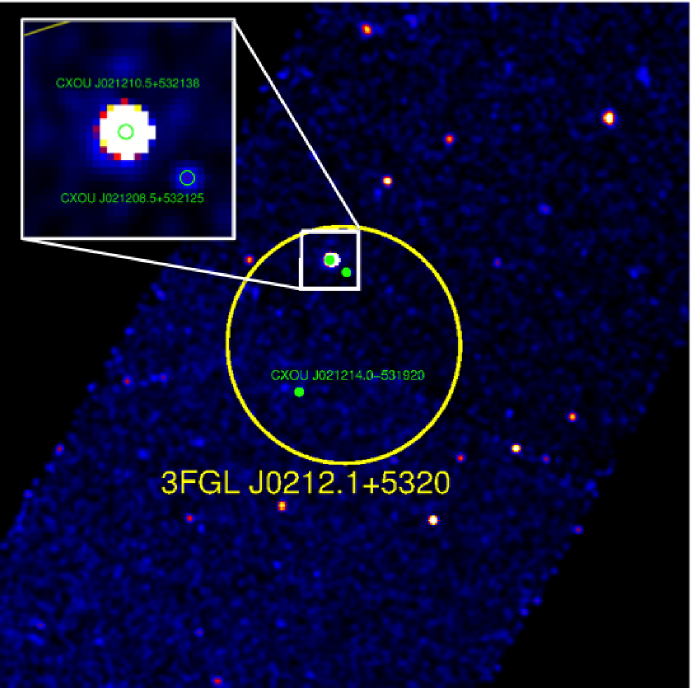
Figure 9: Chandra 30 ks observation of 3FGL J0212.1+5320, predicted by our algorithm to be a millisecond pulsar (MSP, see Table LABEL:unassoc). The smoothed 0.3-10 keV ACIS-I exposure-corrected (10’x10’) image includes the 95% confidence LAT error ellipse (shown in yellow). The most probable X-ray counterpart (CXOU J021210.5+532138) is highlighted in a zoomed 1’x1’ region, with a 2" radius source extraction region shown in green.

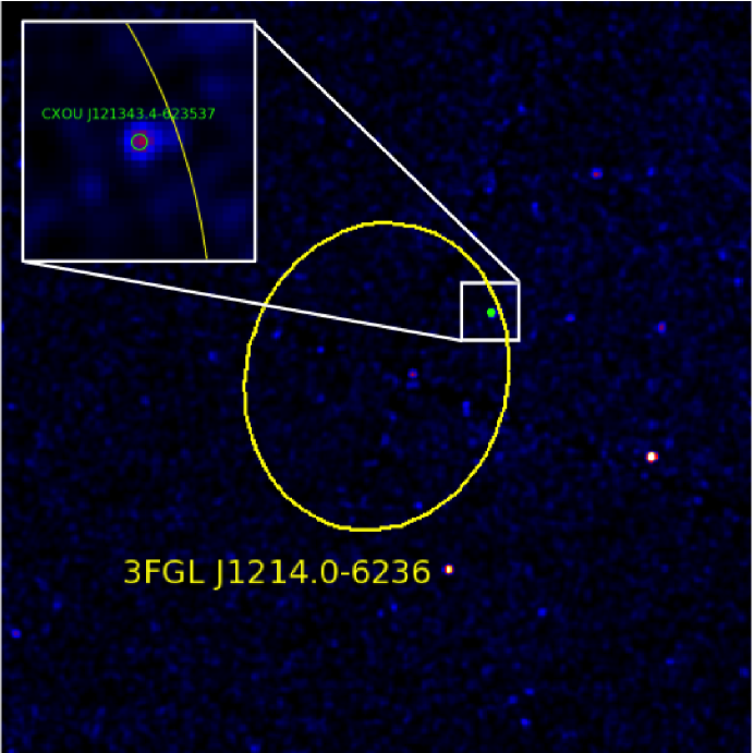
Figure 10: Chandra 20 ks observation of 3FGL J1214.0-6236, coincident with SNR G298.6–0.0, predicted by our algorithm to be a young pulsar (YNG, see Table LABEL:snrpwn). The smoothed 0.3-10 keV ACIS-I exposure-corrected (13’x13’) image includes the 95% confidence LAT error ellipse (shown in yellow). The most probable X-ray counterpart (CXOU J121343.4-623537) is highlighted in a zoomed 1’x1’ region, with a 2" radius source extraction region shown in green.

3FGL J1035.7-6720 and 3FGL J1744.1-7619 were both observed for $\sim$25 ks with XMM (obsIds 0692830201 and 0692830101), and show the presence of possible X-ray counterparts at (RA, DEC) of (158.8652, -67.3371) and (266.0030, -76.3205), respectively. LAT sources 3FGL J0212.1+5320 and 3FGL J0933.9-6232, both strong MSP candidates, were observed with Chandra for $\sim$30 ks (obsid 14814) and $\sim$45 ks (obsid 14813), respectively, and show the nearest possible X-ray counterparts at (33.0439, 53.3607) and (143.5049, -62.5077), within the LAT error ellipse (e.g. see Figure 9). Source 3FGL J1214.0-6236, coincident with SNR G298.6+0.0 was observed with Chandra for $\sim$20 ks (obsid 14889) and shows a potential counterpart at (183.4307, -62.5936), as shown in Figure 10. 3FGL J1405.4-6119, coincident with SNR G311.5+0.3, was observed with Chandra for 13 ks (obsid 14888), showing a possible counterpart at (211.3103, -61.3077).

In addition to the dedicated Chandra and XMM observations, many other LAT sources have been observed with less sensitive instruments. Indeed, since the launch of Fermi, we have been using the Swift X-ray telescope (Gehrels et al., 2004) to carry out follow-up observations of LAT unassociated sources (Stroh & Falcone (2013), Falcone et al. (2016), in preparation), as part of an ongoing multi-year Fermi Guest Investigator program (PI: Falcone). This has resulted, to date (through 2015-12-21), in the detection of almost 1900 sources (with SNR $>$ 3). We selected only those X-ray sources within a radius of 1.2 times the semimajor radius of the 95% confidence region of our best pulsar candidates (those predicted to be pulsars by both the RF and LR methods). Table LABEL:counterparts provides a list of these $\sim$90 potential counterparts. For each potential counterpart we convert the measured count rate into an estimated flux in the 0.1–2.4 keV band by assuming a power law spectrum of index -2 and estimating the Galactic Hydrogen column density using the method of Willingale et al. (2013). Given the known faintness of pulsars in the X-ray band (e.g. Marelli et al., 2011), our flux estimates can be used to likely rule out any bright Swift source (e.g. with flux greater than $\sim 5\times 10^{-13}$ erg cm^-2 s^-1) as a plausible X-ray counterpart of a pulsar While in some cases the Swift observations have been superseded by observations with more sensitive instruments (e.g. 3FGL J0212.1+5320, see previous paragraphs), we nevertheless leave the Swift results in Table LABEL:counterparts for completeness, and possible comparison.

Appendix A Scripts

The following scripts reproduce the key results presented in the previous sections. They can also be obtained at:
http://www.physics.hku.hk/$\sim$pablo/pulsarness.html
and/or:
http://scipp.ucsc.edu/$\sim$pablo/pulsarness.html. The scripts were run on R version 3.2.3, on a Mac running OS X, Version 10.9.5. The following R packages were used: fermicatsR (v1.3), dplyr (v0.4.3), pROC (v1.8), randomForest (v4.6-12), RWeka(v0.4-24), e1071 (v1.6-7), ISLR (v1.0), leaps (v2.9), gam (v1.12), and mgcv (v1.8-9).

A.1 Getting and Cleaning Data

⬇

# Load fermicatsR package containing Fermi LAT Catalogs

library(fermicatsR)

# Load dplyr package for efficient handling of data frames

library(dplyr)

# Define function to compute SED points (energy flux at the geometric mean of the energy band)

sedflux <- function(photon_flux, alpha, Elo, Ehi) {

R <- Elo/Ehi

GeV2erg <- 0.00160217657

(GeV2erg*Elo)*(alpha-1)*(photon_flux)*(R^(alpha/2 - 1))/(1-(R^(alpha-1)))

}

# Subselect small number of variables from those available in 3FGL

FGL3_01 <- select(FGL3,

Source_Name, RAJ2000, DEJ2000, GLON, GLAT,

Spectral_Index, Energy_Flux100, Variability_Index,

Conf_68_SemiMajor, Conf_68_SemiMinor, Conf_68_PosAng,

Conf_95_SemiMajor, Conf_95_SemiMinor, Conf_95_PosAng,

Signif_Avg, Pivot_Energy, Flux_Density, Unc_Flux_Density,

Flux1000, Unc_Flux1000, Energy_Flux100, Unc_Energy_Flux100,

Signif_Curve, Flux100_300, Flux300_1000, Flux1000_3000,

Flux3000_10000, Flux10000_100000, CLASS1, ASSOC1)

# Add new variables (SED points and hardness ratios) computed using sedflux function above

FGL3_02 <- mutate(FGL3_01,

SED100_300 = sedflux(Flux100_300, Spectral_Index, 0.1, 0.3),

SED300_1000 = sedflux(Flux300_1000, Spectral_Index, 0.3, 1.0),

SED1000_3000 = sedflux(Flux1000_3000, Spectral_Index, 1.0, 3.0),

SED3000_10000 = sedflux(Flux3000_10000, Spectral_Index, 3.0, 10.0),

SED10000_100000 = sedflux(Flux10000_100000, Spectral_Index, 10.0, 100.0),

hr12 = (SED300_1000-SED100_300)/(SED300_1000+SED100_300),

hr23 = (SED1000_3000-SED300_1000)/(SED1000_3000+SED300_1000),

hr34 = (SED3000_10000-SED1000_3000)/(SED3000_10000+SED1000_3000),

hr45 = (SED10000_100000-SED3000_10000)/(SED10000_100000+SED3000_10000),

CLASS1 = gsub("␣", "", CLASS1))

# Drop highly correlated and some unused variables

FGL3_03 <- select(FGL3_02,

-Unc_Flux1000, -Energy_Flux100, -Conf_95_SemiMajor, -Conf_95_SemiMinor,

-Flux100_300, -Conf_68_SemiMajor, -Conf_68_SemiMinor, -Conf_68_PosAng,

-Flux1000, -SED100_300, -SED300_1000, -SED1000_3000, -SED3000_10000,

-SED10000_100000, -Flux300_1000, -Flux1000_3000, -Flux3000_10000)

# Take log of variables with highly skewed distributions (removing zeroes to avoid -Inf)

FGL3_04 <- filter(FGL3_03, FGL3_03$Signif_Curve != 0) %>%

mutate(Variability_Index = log(Variability_Index),

Pivot_Energy = log(Pivot_Energy),

Flux_Density = log(Flux_Density),

Unc_Flux_Density = log(Unc_Flux_Density),

Unc_Energy_Flux100 = log(Unc_Energy_Flux100),

Flux10000_100000 = log(Flux10000_100000),

Signif_Curve = log(Signif_Curve))

# Drop a few more unused variables

FGL3_05 <- select(FGL3_04, -Pivot_Energy, -Unc_Flux_Density, -Flux10000_100000)

# Create a tidy data set including "pulsarness" and "agnness" factors

FGL3_tidy <- select(FGL3_05, -RAJ2000, -DEJ2000, -GLON, -Signif_Avg) %>%

mutate(agnness = factor(CLASS1 == "BCU" | CLASS1 == "bcu"

|CLASS1 == "BLL" | CLASS1 == "bll"

|CLASS1 == "FSRQ"| CLASS1 == "fsrq"

|CLASS1 == "rdg" | CLASS1 == "RDG"

|CLASS1 == "nlsy1" | CLASS1 == "NLSY1"

|CLASS1 == "agn" | CLASS1 == "ssrq"

|CLASS1 == "sey",

labels = c("Non-AGN", "AGN")),

pulsarness = factor(CLASS1 == "PSR" | CLASS1 == "psr",

labels = c("Non-Pulsar", "Pulsar")))

# Create the FGL3_results data frame that will contain final results

FGL3_results <- select(FGL3_05, Source_Name,

Signif = Signif_Avg,

Flux = Flux_Density,

RA = RAJ2000,

DEC = DEJ2000,

GLON, GLAT, ASSOC1, CLASS1) %>%

mutate(Source_Name = substr(Source_Name, 6, 18),

RA = format(RA, digits = 2),

DEC = format(DEC, digits = 2),

GLON = format(GLON, digits = 2),

GLAT = format(GLAT, digits = 2),

Signif = round(Signif, digits = 3)) %>%

mutate(Flux = format(exp(Flux), scientific = TRUE, digits = 3))

# Select data for PSR (pulsarness == "Pulsar") vs AGN (agnness == "AGN") classification

FGL3_AGNPSR <- filter(FGL3_tidy, pulsarness == "Pulsar" | agnness == "AGN")

# Drop sources with missing values and some unused variables

FGL3_AGNPSR <- na.omit(FGL3_AGNPSR)

FGL3_AGNPSR <- select(FGL3_AGNPSR, -CLASS1, -ASSOC1, -Source_Name,

-GLAT, -Conf_95_PosAng, -agnness)

# Set Random seed

set.seed(1)

# Separate into training (70%) and testing (30%) sets

train <- sample(nrow(FGL3_AGNPSR), round(nrow(FGL3_AGNPSR)*0.7))

FGL3_test <- FGL3_AGNPSR[-train, ]

FGL3_train <- FGL3_AGNPSR[train, ]

# Split training data into k (10) blocks for k-fold cross-validation

k <- 10

Index <- sample(nrow(FGL3_train))

Block_index <- matrix(data = Index[1:(floor(nrow(FGL3_train)/k)*k)], nrow = k, byrow = TRUE)

FGL3_train_CV <- FGL3_train[Index[1:(floor(nrow(FGL3_train)/k)*k)], ]

# Initialise predictions vector

predictions_FGL3_train_CV <- rep(0, nrow(FGL3_train_CV))

# Prepare pulsar data sets for YNG vs MSP classification

pulsars_long <- mutate(pulsars, PSR_coords = substr(PSR, 6, 12))

FGL3_pulsars <- FGL3_tidy %>%

filter(pulsarness == "Pulsar") %>%

mutate(ASSOC1 = as.character(ASSOC1))

a <- strsplit(FGL3_pulsars$ASSOC1, "PSR␣J")

b <- character(nrow(FGL3_pulsars))

for (i in 1:nrow(FGL3_pulsars)) {

b[i] <- gsub("␣", "", a[[i]][2])

}

FGL3_pulsars$ASSOC1_code <- b

FGL3_pulsars <- mutate(FGL3_pulsars, ASSOC1_code = substr(ASSOC1_code, 1, 7))

bothFGL3andpulsars <- inner_join(pulsars_long, FGL3_pulsars,

by = c("PSR_coords" = "ASSOC1_code"))

FGL3_Pulsars <- mutate(bothFGL3andpulsars,

pulsarness = factor(P_ms >= 10, labels = c("MSP", "YNG"))) %>%

select(-P_ms, -Codes, -RAJ_deg, -DECJ_deg, -Refs, -CLASS1, -ASSOC1,

-Source_Name, -PSR, -PSR_coords, -Edot, -agnness)

# Separate pulsar data set into 30% (testing test) and 70% (training test)

set.seed (1)

train <- sample(nrow(FGL3_Pulsars), round(nrow(FGL3_Pulsars)*0.7))

FGL3_Pulsars_test <- FGL3_Pulsars[-train, ]

FGL3_Pulsars_train <- FGL3_Pulsars[train, ]

# Clean up and Set aside required data sets

Environ <- ls()

Environ <- Environ[Environ != "FGL3_tidy"

& Environ != "FGL3_results"

& Environ != "FGL3_test"

& Environ != "FGL3_train"

& Environ != "predictions_FGL3_train_CV"

& Environ != "Block_index"

& Environ != "FGL3_train_CV"

& Environ != "FGL3_Pulsars_train"

& Environ != "FGL3_Pulsars_test"]

rm(list = Environ)

# Save current workspace for subsequent steps

save.image()

A.2 Function to get best threshold, plot ROC curves and print tables

⬇

# Load workspace from previous step

load(".RData")

# Load pROC package

library(pROC)

# Function to get the best threshold

ROC_threshold <- function(truth, prediction) {

ROC <- roc(truth, prediction)

ROC_table <- cbind(ROC$thresholds, ROC$specificities, ROC$sensitivities)

ROC_table[which.max(ROC_table[, 2] + ROC_table[, 3]), ]

}

# Function to plot ROC curves

ROC_plots <- function(truth_train, prediction_train, truth_test, prediction_test) {

par(mfrow = c(1, 2))

ROC_train <- roc(truth_train, prediction_train,

plot = TRUE, print.auc = TRUE, main = "ROC␣Train", print.thres = "best")

ROC_test <- roc(truth_test, prediction_test,

plot = TRUE, print.auc = TRUE, main = "ROC␣Test", print.thres = "best")

}

# Function to generate contingency tables

ROC_tables <- function(truth_train, prediction_train, truth_test, prediction_test,

cat1 = "Pulsar", cat2 = "AGN") {

ROC <- roc(truth_train, prediction_train)

ROC_table <- cbind(ROC$thresholds, ROC$specificities, ROC$sensitivities)

threshold <- ROC_table[which.max(ROC_table[, 2] + ROC_table[, 3]), ]

# Training data

nrow_train <- length(prediction_train)

Predict_class_train <- rep("NA", nrow_train)

Predict_class_train <- ifelse(prediction_train > threshold[1], cat1, cat2)

real_category <- truth_train

print(table(Predict_class_train, real_category))

# Testing data

nrow_test <- length(prediction_test)

Predict_class_test <- rep("NA", nrow_test)

Predict_class_test <- ifelse(prediction_test > threshold[1], cat1, cat2)

real_category <- truth_test

print(table(Predict_class_test, real_category))

}

ROC_threshold_plots_tables <- function(truth_train, prediction_train, truth_test, prediction_test,

threshold = 0, cat1 = "Pulsar", cat2 = "AGN") {

if (threshold == 0) {

# Compute best threshold if none is provided

ROC <- roc(truth_train, prediction_train)

ROC_table <- cbind(ROC$thresholds, ROC$specificities, ROC$sensitivities)

best_threshold <- ROC_table[which.max(ROC_table[, 2] + ROC_table[, 3]), ]

} else {

# Don't compute threshold if one is provided

best_threshold <- threshold

}

if (nargs() > 2) {

# Make ROC plots

par(mfrow = c(1, 2))

ROC_train <- roc(truth_train, prediction_train,

plot = TRUE, print.auc = TRUE, main = "ROC␣Train", print.thres = "best")

ROC_test <- roc(truth_test, prediction_test,

plot = TRUE, print.auc = TRUE, main = "ROC␣Test", print.thres = "best")

# Generate contingency tables

# Training data

nrow_train <- length(prediction_train)

Predict_class_train <- rep("NA", nrow_train)

Predict_class_train <- ifelse(prediction_train > best_threshold[1], cat1, cat2)

real_category <- truth_train

print(table(Predict_class_train, real_category))

# Testing data

nrow_test <- length(prediction_test)

Predict_class_test <- rep("NA", nrow_test)

Predict_class_test <- ifelse(prediction_test > best_threshold[1], cat1, cat2)

real_category <- truth_test

print(table(Predict_class_test, real_category))

}

return(best_threshold)

}

# Function to get best threshold, plot ROC curves and print tables

ROCandTable <- function(predictions_FGL3_train, FGL3_train,

predictions_FGL3_test, FGL3_test, Best_threshold) {

# Plot ROC curve and Table for train and testing data

par(mfrow = c(1, 2))

# Draw ROC for train_data

ROC_FGL3_train <- roc(FGL3_train$pulsarness, predictions_FGL3_train,

plot = TRUE, print.auc = TRUE, main = "ROC␣FGL3␣Train",

print.thres = "best")

# Draw ROC for test_data

ROC_FGL3_test <- roc(FGL3_test$pulsarness, predictions_FGL3_test,

plot = TRUE, print.auc = TRUE, main="ROC␣FGL3␣Test",

print.thres = "best")

# Using The Best Threshold from cross-validation method

Best_threshold

# Table for training data

nrow_train <- nrow(FGL3_train)

Predict_class <- rep("NA", nrow_train)

for (i in 1:nrow_train) {

if (predictions_FGL3_train[i] <= Best_threshold[1]) {

Predict_class[i] <- "AGN"

} else {

Predict_class[i] <- "Pulsar"

}

}

real_category <- FGL3_train$pulsarness

print(table(Predict_class, real_category))

# Table for testing data

nrow_test <- nrow(FGL3_test)

Predict_class <- rep("NA", nrow_test)

for (i in 1:nrow_test) {

if (predictions_FGL3_test[i] <= Best_threshold[1]){

Predict_class[i] <- "AGN"

} else {

Predict_class[i] <- "Pulsar"

}

}

real_category <- FGL3_test$pulsarness

print(table(Predict_class, real_category))

}

# Save current workspace for subsequent steps

save.image()

A.3 AGN vs PSR classification using Logistic Regression (LR) model (backward stepwise selection)

⬇

# AGN vs PSR classification using Logistic Regression (LR) model (backward stepwise selection)

# Load workspace from previous step

load(".RData")

# Load pROC package

library(pROC)

null <- glm(pulsarness ~1, family = binomial, data = FGL3_train)

glm.step.backward.AIC <- step(glm(pulsarness ~., family = binomial, data = FGL3_train),

scope = list(lower = null, upper = glm(pulsarness ~.,

family = binomial, data = FGL3_train)),

direction = "backward")

print(summary(glm.step.backward.AIC))

predictions_FGL3_train <- predict(glm.step.backward.AIC, FGL3_train, type = "response")

predictions_FGL3_test <- predict(glm.step.backward.AIC, FGL3_test, type = "response")

# Get Training Set threshold, generate ROC plots, and print contingency tables

Best_threshold_train <- ROC_threshold_plots_tables(FGL3_train$pulsarness,

predictions_FGL3_train,

FGL3_test$pulsarness,

predictions_FGL3_test)

# Add LR Prediction Probabilities to FGL3_results data frame:

FGL3_results$LR_P <- round(predict(glm.step.backward.AIC, FGL3_tidy,

type = "response"), digits = 3)

# Add LR Prediction category to FGL3_results data frame:

FGL3_results$LR_Pred <- ifelse(FGL3_results$LR_P > Best_threshold_train[1],

"PSR", "AGN")

# Clean up and Set aside required data sets

Environ <- ls()

Environ <- Environ[Environ != "FGL3_tidy"

& Environ != "FGL3_results"

& Environ != "FGL3_test"

& Environ != "FGL3_train"

& Environ != "predictions_FGL3_train_CV"

& Environ != "Block_index"

& Environ != "FGL3_train_CV"

& Environ != "ROC_threshold_plots_tables"

& Environ != "FGL3_Pulsars_train"

& Environ != "FGL3_Pulsars_test"]

rm(list = Environ)

# Save current workspace for subsequent steps

save.image()

A.4 AGN vs PSR classification using Random Forests (RF)

⬇

# AGN vs PSR classification using Random Forests (RF)

# Load workspace from previous step

load(".RData")

# Load randomForest package

library(randomForest)

set.seed(1)

# First use 10-fold cross validation method to fit models and get the forecast of each block of data

k <- 10

for (i in 1:k) {

Model <- randomForest(pulsarness~., data = FGL3_train[-Block_index[i, ], ], importance = TRUE)

predictions_FGL3_train_CV[((i-1)*(nrow(FGL3_train_CV)/k) + 1):((i)*(nrow(FGL3_train_CV)/k))] <-

predict(Model, newdata = FGL3_train[Block_index[i, ], ], type = "Prob")[, 2]

print(i)

}

# Get best threshold

Best_threshold_train_CV <- ROC_threshold_plots_tables(FGL3_train_CV$pulsarness,

predictions_FGL3_train_CV)

# Now Modeling using all the data

rf.full.FGL3 <- randomForest(pulsarness~., data = FGL3_train, importance = TRUE)

# The importance of each variable

importance(rf.full.FGL3)

varImpPlot(rf.full.FGL3)

# Prediction for train and test

predictions_FGL3_train <- predict(rf.full.FGL3, newdata = FGL3_train, type = "Prob")[, 2]

predictions_FGL3_test <- predict(rf.full.FGL3, newdata = FGL3_test, type = "Prob")[,2 ]

# Generate ROC plots, and print contingency tables

ROC_threshold_plots_tables(FGL3_train$pulsarness, predictions_FGL3_train,

FGL3_test$pulsarness, predictions_FGL3_test, threshold = Best_threshold_train_CV[1])

cat("Best␣threshold␣from␣cross-validation:", Best_threshold_train_CV)

# Add RF Prediction probabilities to FGL3_results

FGL3_results$RF_P <- predict(rf.full.FGL3, newdata = FGL3_tidy, type = "Prob")[,2 ]

#FGL3_results <- mutate(FGL3_results, RF_P)

# Add RF Prediction category to FGL3_results

FGL3_results$RF_Pred <- ifelse(FGL3_results$RF_P > Best_threshold_train_CV[1],

c("PSR"), c("AGN"))

# Plot for the paper

par(mfrow = c(1,1))

varImpPlot(rf.full.FGL3, pch = 19, type = 1, main = "")

# Clean up and Set aside required data sets

Environ <- ls()

Environ <- Environ[Environ != "FGL3_tidy"

& Environ != "FGL3_results"

& Environ != "FGL3_test"

& Environ != "FGL3_train"

& Environ != "predictions_FGL3_train_CV"

& Environ != "Block_index"

& Environ != "FGL3_train_CV"

& Environ != "ROC_threshold_plots_tables"

& Environ != "FGL3_Pulsars_train"

& Environ != "FGL3_Pulsars_test"

& Environ != "rf.full.FGL3"]

rm(list = Environ)

# Save current workspace for subsequent steps

save.image()

A.5 Outlyingness

⬇

# Computation of AGN and PSR "outlyingness" using Random Forests (RF)

# Load workspace from previous step

load(".RData")

# Load randomForest package

library(randomForest)

# Set random seed

set.seed(1)

# Compute RF predictions on entire FGL3 data

results <- predict(rf.full.FGL3, newdata = FGL3_tidy, proximity = TRUE, type = "Prob")

# Use proximity matrix to compute PSR and AGN "outlyingness"

nobs <- dim(FGL3_tidy)[1]

PSR_Out <- numeric(nobs)

AGN_Out <- numeric(nobs)

for (i in 1:nobs ) {

PSR_proximities <- results$proximity[FGL3_tidy$pulsarness == "Pulsar", i]

PSR_Out[i] <- 1./sum(PSR_proximities^2)

AGN_proximities <- results$proximity[FGL3_tidy$agnness == "AGN", i]

AGN_Out[i] <- 1./sum(AGN_proximities^2)

}

# Normalize outlyingness

PSR_Out_norm <- (PSR_Out - median(PSR_Out[FGL3_tidy$pulsarness == "Pulsar"])) /

mad(PSR_Out[FGL3_tidy$pulsarness=="Pulsar"])

AGN_Out_norm <- (AGN_Out - median(AGN_Out[FGL3_tidy$agnness == "AGN"])) /

mad(AGN_Out[FGL3_tidy$agnness=="AGN"])

# Add outlyingness to FGL3_results data frame

FGL3_results$PSR_Out <- round(PSR_Out_norm, digits = 3)

FGL3_results$AGN_Out <- round(AGN_Out_norm, digits = 3)

# Clean up and Set aside required data sets

Environ <- ls()

Environ <- Environ[Environ != "FGL3_tidy"

& Environ != "FGL3_results"

& Environ != "FGL3_test"

& Environ != "FGL3_train"

& Environ != "predictions_FGL3_train_CV"

& Environ != "Block_index"

& Environ != "FGL3_train_CV"

& Environ != "ROC_threshold_plots_tables"

& Environ != "FGL3_Pulsars_train"

& Environ != "FGL3_Pulsars_test"]

rm(list = Environ)

# Save current workspace for subsequent steps

save.image()

A.6 Pulsar (YNG vs MSP) classification using Boosted LR

⬇

# Pulsar (YNG vs MSP) classification using Boosted LR

# Load workspace from previous step

load(".RData")

# Load RWeka and pROC packages

library(RWeka)

library(pROC)

# WOW(LogitBoost)

Model <- LogitBoost(pulsarness ~., data = FGL3_Pulsars_train)

summary(Model)

# Model predictions

predictions_FGL3_Pulsars_train <- predict(Model,

newdata = FGL3_Pulsars_train, type = "probability")[, 2]

predictions_FGL3_Pulsars_test <- predict(Model,

newdata = FGL3_Pulsars_test, type = "probability")[, 2]

# Generate ROC plots and print contingency tables

Best_threshold_train <- ROC_threshold_plots_tables(FGL3_Pulsars_train$pulsarness,

predictions_FGL3_Pulsars_train,

FGL3_Pulsars_test$pulsarness,

predictions_FGL3_Pulsars_test,

cat1 = "YNG", cat2 = "MSP")

# Add Boosted Logistic Regression Prediction probabilities to FGL3_results data frame

FGL3_results$Blogistic_YNG_P <- round(predict(Model,

newdata = FGL3_tidy, type = "probability")[, 2],

digits = 3)

# Add Boosted Logistic Regression Prediction category to FGL3_results data frame

FGL3_results$Blogistic_YNG_Pred <- ifelse(FGL3_results$Blogistic_YNG_P > Best_threshold_train[1],

c("YNG"), c("MSP"))

# Clean up and Set aside required data sets

Environ <- ls()

Environ <- Environ[Environ != "FGL3_tidy"

& Environ != "FGL3_results"

& Environ != "FGL3_test"

& Environ != "FGL3_train"

& Environ != "predictions_FGL3_train_CV"

& Environ != "Block_index"

& Environ != "FGL3_train_CV"

& Environ != "ROC_threshold_plots_tables"

& Environ != "FGL3_Pulsars_train"

& Environ != "FGL3_Pulsars_test"]

rm(list = Environ)

# Save current workspace for subsequent steps

save.image()

A.7 Pulsar (YNG vs MSP) classification using Random Forests (RF)

⬇

# Pulsar (YNG vs MSP) classification using Random Forests (RF)

# Load workspace from previous step

load(".RData")

# Load randomForest and pROC packages

library(randomForest)

library(pROC)

# Set random seed

set.seed(1)

# Full model

rf.P <- randomForest(pulsarness ~., data = FGL3_Pulsars_train, importance = TRUE)

# The importance of each variable

importance(rf.P)

varImpPlot(rf.P)

# Model predictions

predictions_FGL3_Pulsars_train <- predict(rf.P,

newdata = FGL3_Pulsars_train, type = "Prob")[,2 ]

predictions_FGL3_Pulsars_test <- predict(rf.P,

newdata = FGL3_Pulsars_test, type = "Prob")[,2 ]

# Generate ROC plots and print contingency tables

Best_threshold_train <- ROC_threshold_plots_tables(FGL3_Pulsars_train$pulsarness,

predictions_FGL3_Pulsars_train,

FGL3_Pulsars_test$pulsarness,

predictions_FGL3_Pulsars_test,

cat1 = "YNG", cat2 = "MSP")

# Add RF Prediction probabilities to FGL3_results data frame

FGL3_results$RF_YNG_P <- round(predict(rf.P,

newdata = FGL3_tidy, type = "Prob")[,2 ],

digits = 3)

# Add RF Prediction category to FGL3_results data frame

FGL3_results$RF_YNG_Pred <- ifelse(FGL3_results$RF_YNG_P > Best_threshold_train[1],

c("YNG"), c("MSP"))

# Plot Importance

par(mfrow = c(1,1))

varImpPlot(rf.P, pch = 19, type = 1, main = "")

# Clean up and Set aside required data sets

Environ <- ls()

Environ <- Environ[Environ != "FGL3_tidy"

& Environ != "FGL3_results"

& Environ != "FGL3_test"

& Environ != "FGL3_train"

& Environ != "predictions_FGL3_train_CV"

& Environ != "Block_index"

& Environ != "FGL3_train_CV"

& Environ != "ROC_threshold_plots_tables"

& Environ != "FGL3_Pulsars_train"

& Environ != "FGL3_Pulsars_test"]

rm(list = Environ)

# Save current workspace for subsequent steps

save.image()

# Write results to a file

save(FGL3_results, file = "FGL3_results.rdata", compress = "xz")

Table 1: Predictor Parameters used for the AGN vs PSR models.

Parameter	Min.	Median	Max.
Spectral_Index	0.5	2.2	3.1
Variability_Index	3.0	4.0	11.0
Flux_Density	-35.4	-28.2	-19.9
Unc_Energy_Flux100	-28.5	-27.6	-24.8
Signif_Curve	-5.8	0.4	4.4
$hr_{12}$	-1	-0.1	1
$hr_{23}$	-1	-0.1	1
$hr_{34}$	-1	-0.2	1
$hr_{45}$	-1	-0.3	1

Table 2: Performance of the algorithms in classifying AGN vs PSR, based on a testing sample of 521 AGN and 50 PSR (in bold are the two best methods, Random Forest (RF) and Logistic Regression (LR), as described in Sections 3.1 and 3.2)).

Model	AGN	PSR	PSR	Overall	F1
	Test Errors	Test Errors	Sensitivity	Accuracy	Score
	(out of 521)	(out of 50)
LR (forward stepwise)	38	1	98%	93.2%	71.5%
LR (backward stepwise)	29	1	98%	94.7%	76.6%
Decision Tree (C4.5)	15	6	88%	96.3%	80.7%
Two-stage	17	6	88%	96.0%	79.3%
GAM	25	4	92%	94.9%	76.0%
SVM (CV)	29	1	98%	94.8%	76.6%
LR (CV)	31	1	98%	94.4%	75.4%
Boosted LR (CV)	24	5	90%	94.9%	75.6%
Logistic Trees (CV)	36	2	96%	93.4%	71.6%
Decision Tree (C4.5 with CV)	15	6	88%	96.3%	80.7%
RF (CV)	17	2	96%	96.7%	83.5%

Table 3: Performance of the algorithms in classifying Young (YNG) vs Millisecond pulsars (MSP), based on a testing sample of 25 YNG and 18 MSP (in bold are the two best methods, RF and Boosted LR, described in Sections 3.1 and 3.3).

Model	YNG	MSP	Overall
	Test Errors	Test Errors	Accuracy
	(out of 25)	(out of 18)
LR (forward stepwise)	7	2	79.1%
LR (backward stepwise)	7	2	79.1%
Boosted LR	2	2	90.7%
Logistic Trees	7	2	79.1%
GAM	2	4	86.1%
SVM	4	3	83.7%
Decision Tree (C4.5)	7	0	83.7%
RF	2	2	90.7%

Table 4: Predictor parameters for the logistic regression model (backwards stepwise)

Parameter	Estimate	Std. Error	z value	Pr($>|z|$)
(Intercept)	151.7880	23.5877	6.435	1.23e-10
Variability_Index	-5.5473	0.9253	-5.995	2.03e-09
Unc_Energy_Flux100	3.7512	0.6978	5.376	7.64e-08
hr45	-4.3291	0.9729	-4.450	8.59e-06
hr34	-4.2981	1.3213	-3.253	0.00114
Spectral_Index	-5.8615	1.8620	-3.148	0.00164
Flux_Density	0.7541	0.2726	2.766	0.00567
Signif_Curve	1.2275	0.5569	2.204	0.02750
hr23	1.7846	1.1325	1.576	0.11506

Table 5: Results of our best models, as applied to the 3FGL catalog (all 3021 sources for which predictor parameters are available, for which our models could therefore be applied). The table is published in its entirety in the electronic edition of the article. A portion is shown here for guidance regarding its form and content. The columns are: 3FGL Name (Source_Name), 4-year significance (Signif), Flux Density, in photon/cm2/MeV/s (Flux), RA, DEC, Galactic Longitude and Latitude (GLON, GLAT), Name of identified or likely associated source (ASSOC1), class designation from 3FGL catalog (CLASS1), LR Probability and predicted class (LR_P, Pred), RF Probability and predicted class (RF_P, Pred), PSR Outlyingness (PSR_Out), AGN Outlyingness (AGN_Out), Boosted LR Probability (of being a YNG pulsar) and predicted pulsar class (BLR_P, BLR_Pred), and RF Probability (of being a YNG pulsar) and predicted pulsar class (RF_P and RF_Pred).

Source_Name	Signif	Flux	RA	DEC	GLON	GLAT	ASSOC1	CLASS1	LR	LR	RF	RF	PSR	AGN	BLR	BLR	RF	RF
3FGL									P	Pred	P	Pred	Out	Out	P	Pred	P	Pred
J0000.1+6545	6.81	1.01e-12	0.038	65.7517	117.69	3.4030			0.38	PSR	0.19	PSR	203.05	10.79	0.22	MSP	0.52	YNG
J0000.2-3738	5.09	1.94e-14	0.061	-37.6484	345.41	-74.9468			0.00	AGN	0.00	AGN	109.49	-0.63	0.00		0.13
J0001.0+6314	6.16	8.62e-12	0.254	63.2440	117.29	0.9257		spp	0.00	AGN	0.05	AGN	187.32	4.20	0.16		0.41
J0001.2-0748	11.25	4.85e-13	0.321	-7.8159	89.02	-67.3242	PMN J0001-0746	bll	0.02	AGN	0.01	AGN	81.14	2.64	0.00		0.04
J0001.4+2120	11.35	2.52e-11	0.361	21.3379	107.67	-40.0472	TXS 2358+209	fsrq	0.00	AGN	0.00	AGN	203.17	1.55	0.01		0.32
J0001.6+3535	4.20	2.87e-13	0.404	35.5905	111.66	-26.1885			0.00	AGN	0.04	AGN	194.12	0.33	0.00		0.17
J0002.0-6722	5.89	4.83e-14	0.524	-67.3703	310.14	-49.0618			0.00	AGN	0.00	AGN	100.44	-0.72	0.00		0.13
J0002.2-4152	5.16	7.32e-14	0.562	-41.8828	334.07	-72.1427	1RXS J000135.5-415519	bcu	0.00	AGN	0.00	AGN	120.90	-0.78	0.00		0.16
J0002.6+6218	17.97	4.30e-12	0.674	62.3006	117.30	-0.0371			0.99	PSR	0.81	PSR	1.98	751.35	0.82	YNG	0.54	YNG
J0003.2-5246	5.67	2.00e-14	0.815	-52.7771	318.98	-62.8247	RBS 0006	bcu	0.00	AGN	0.00	AGN	148.05	-0.61	0.00		0.13
J0003.4+3100	6.29	2.03e-12	0.858	31.0085	110.96	-30.7451			0.15	PSR	0.08	AGN	181.42	15.50	0.01	MSP	0.17	MSP
J0003.5+5721	5.38	1.09e-13	0.890	57.3597	116.49	-4.9116			0.04	AGN	0.04	AGN	206.61	1.63	0.01		0.24
J0003.8-1151	4.18	4.42e-14	0.959	-11.8627	84.43	-71.0842	PMN J0004-1148	bcu	0.00	AGN	0.02	AGN	109.97	0.04	0.00		0.12
J0004.2+6757	6.01	6.01e-13	1.055	67.9593	118.51	5.4940			0.67	PSR	0.54	PSR	76.78	218.93	0.49	MSP	0.39	MSP

Table 6: List of the most significant 3FGL unassociated sources predicted by both RF and LR to be pulsars. Column definitions are the same as in Table 5. LR_P and RF_P give the probabilities of being a pulsar (according to the LR and RF algorithms), while the last two columns give the predicted type of pulsar (according to the BLR and RF algorithms, respectively). In bold we highlight two recently-discovered pulsars and four strong millisecond pulsar candidates (see text for details).

	Source_Name	Signif	RA	DEC	LR_P	RF_P	BLR/RF Pred
1	3FGL J1744.1-7619	32.85	266.045	-76.3286	1.00	0.96	MSP/MSP
2	3FGL J1653.6-0158	31.95	253.419	-1.9801	0.99	0.73	MSP/MSP
3	3FGL J1035.7-6720	30.48	158.926	-67.3335	1.00	0.94	MSP/MSP
4	3FGL J1119.9-2204	30.16	169.984	-22.0673	0.99	0.91	MSP/MSP
5	3FGL J2112.5-3044	30.14	318.145	-30.7344	0.99	0.94	MSP/MSP
6	3FGL J1702.8-5656	28.81	255.720	-56.9357	0.92	0.36	MSP/MSP
7	3FGL J1625.1-0021	28.53	246.279	-0.3586	1.00	0.98	MSP/MSP
8	3FGL J1906.6+0720	26.27	286.671	7.3339	1.00	0.85	YNG/YNG
9	3FGL J0523.3-2528	26.14	80.839	-25.4763	0.52	0.36	MSP/MSP
10	3FGL J1306.4-6043	25.45	196.615	-60.7317	1.00	0.90	MSP/MSP
11	3FGL J2039.6-5618	25.38	309.918	-56.3121	0.99	0.82	MSP/MSP
12	3FGL J0212.1+5320	25.07	33.037	53.3360	0.98	0.92	MSP/MSP
13	3FGL J2017.9+3627	25.04	304.485	36.4591	1.00	0.85	YNG/YNG
14	3FGL J1405.4-6119	24.82	211.356	-61.3168	1.00	0.77	YNG/YNG
15	3FGL J0340.4+5302	22.31	55.100	53.0484	0.99	0.28	YNG/YNG
16	3FGL J0933.9-6232	22.07	143.481	-62.5338	0.99	0.96	MSP/MSP
17	3FGL J0634.1+0424	21.06	98.528	4.4062	0.98	0.69	YNG/YNG
18	3FGL J1745.3-2903c	20.66	266.343	-29.0630	1.00	0.87	YNG/YNG
19	3FGL J1622.9-5004	20.65	245.726	-50.0753	0.99	0.75	YNG/YNG
20	3FGL J1946.4-5403	20.29	296.614	-54.0570	0.98	0.96	MSP/MSP
21	3FGL J1747.0-2828	20.26	266.775	-28.4819	1.00	0.73	YNG/YNG
22	3FGL J1624.2-4041	19.27	246.059	-40.6865	0.99	0.85	YNG/YNG
23	3FGL J1539.2-3324	19.23	234.823	-33.4142	0.96	0.93	MSP/MSP
24	3FGL J0359.5+5413	19.17	59.881	54.2220	1.00	0.83	MSP/YNG
25	3FGL J0954.8-3948	18.89	148.712	-39.8087	0.86	0.26	MSP/MSP
26	3FGL J1848.4-0141	18.67	282.118	-1.6927	1.00	0.73	YNG/YNG
27	3FGL J2004.4+3338	18.46	301.103	33.6451	0.66	0.20	MSP/YNG
28	3FGL J2041.1+4736	18.38	310.281	47.6030	0.99	0.43	YNG/YNG
29	3FGL J0854.8-4503	18.21	133.711	-45.0616	0.98	0.82	YNG/YNG
30	3FGL J0744.1-2523	18.10	116.045	-25.3994	0.97	0.38	MSP/YNG
31	3FGL J0002.6+6218	17.97	0.674	62.3006	0.99	0.81	YNG/YNG
32	3FGL J0336.1+7500	17.75	54.044	75.0153	0.95	0.72	MSP/MSP
33	3FGL J1800.8-2402	17.48	270.222	-24.0351	0.98	0.77	YNG/YNG
34	3FGL J1754.0-2538	16.84	268.508	-25.6486	0.95	0.79	YNG/YNG
35	3FGL J1823.2-1339	16.64	275.820	-13.6513	1.00	0.80	YNG/YNG
36	3FGL J1208.4-6239	16.23	182.120	-62.6612	0.98	0.75	YNG/YNG
37	3FGL J1650.3-4600	16.18	252.599	-46.0141	0.99	0.84	YNG/YNG
38	3FGL J1056.7-5853	16.11	164.179	-58.8960	1.00	0.67	YNG/YNG
39	3FGL J1112.0-6135	15.69	168.017	-61.5842	0.97	0.65	YNG/YNG
40	3FGL J0914.5-4736	15.57	138.641	-47.6152	0.50	0.39	YNG/YNG
41	3FGL J1358.5-6025	15.43	209.643	-60.4298	1.00	0.70	YNG/YNG
42	3FGL J1104.9-6036	15.40	166.248	-60.6091	1.00	0.85	YNG/YNG
43	3FGL J0545.6+6019	15.39	86.415	60.3219	0.56	0.37	MSP/MSP
44	3FGL J1742.6-3321	15.31	265.665	-33.3562	1.00	0.83	YNG/YNG
45	3FGL J1857.9+0210	15.19	284.490	2.1704	1.00	0.85	YNG/YNG
46	3FGL J1740.5-2843	15.13	265.125	-28.7170	1.00	0.76	YNG/YNG
47	3FGL J1748.3-2815c	15.11	267.092	-28.2589	0.98	0.78	YNG/YNG
48	3FGL J1754.0-2930	15.03	268.500	-29.5059	0.99	0.65	YNG/YNG
49	3FGL J0238.0+5237	14.99	39.505	52.6256	0.97	0.65	MSP/MSP
50	3FGL J1839.3-0552	14.92	279.848	-5.8816	1.00	0.88	YNG/YNG
51	3FGL J2117.6+3725	14.50	319.421	37.4256	0.98	0.30	MSP/MSP
52	3FGL J0419.1+6636	14.47	64.778	66.6049	0.26	0.33	MSP/MSP
53	3FGL J2212.5+0703	14.28	333.147	7.0598	0.69	0.40	MSP/MSP
54	3FGL J1447.3-5800	14.23	221.831	-58.0049	1.00	0.61	YNG/YNG
55	3FGL J0426.7+5437	14.19	66.681	54.6168	1.00	0.71	YNG/YNG
56	3FGL J0858.6-4357	14.13	134.657	-43.9582	0.94	0.56	YNG/YNG
57	3FGL J0953.7-1510	14.00	148.429	-15.1745	0.97	0.88	MSP/MSP
58	3FGL J1901.5-0126	13.97	285.399	-1.4481	0.31	0.26	YNG/YNG
59	3FGL J1624.1-4700	13.90	246.042	-47.0058	0.88	0.58	YNG/YNG
60	3FGL J0838.8-2829	13.74	129.704	-28.4892	0.60	0.57	MSP/MSP
61	3FGL J1852.8+0158	13.71	283.209	1.9722	0.98	0.78	YNG/YNG
62	3FGL J1317.6-6315	13.53	199.403	-63.2598	0.97	0.64	YNG/YNG
63	3FGL J1231.6-5113	13.45	187.902	-51.2210	0.99	0.39	YNG/MSP
64	3FGL J1641.5-5319	13.22	250.378	-53.3237	0.99	0.57	YNG/MSP
65	3FGL J1120.6+0713	13.18	170.172	7.2235	0.11	0.45	MSP/MSP
66	3FGL J1026.2-5730	13.14	156.560	-57.5166	0.96	0.85	YNG/YNG
67	3FGL J1843.7-0322	13.09	280.928	-3.3772	1.00	0.70	YNG/YNG
68	3FGL J0223.6+6204	12.88	35.906	62.0811	1.00	0.86	YNG/YNG
69	3FGL J0737.2-3233	12.87	114.314	-32.5588	0.98	0.51	YNG/MSP
70	3FGL J1503.5-5801	12.80	225.893	-58.0294	0.92	0.51	YNG/YNG
71	3FGL J0318.1+0252	12.76	49.536	2.8695	0.88	0.82	MSP/MSP
72	3FGL J1740.5-2726	12.75	265.134	-27.4500	1.00	0.70	YNG/YNG
73	3FGL J2233.1+6542	12.69	338.279	65.7148	0.98	0.32	YNG/YNG
74	3FGL J1857.2+0059	12.39	284.310	0.9863	0.99	0.79	YNG/YNG
75	3FGL J2103.7-1113	12.33	315.942	-11.2291	0.30	0.42	MSP/MSP
76	3FGL J0802.3-5610	12.31	120.583	-56.1688	0.87	0.41	MSP/MSP
77	3FGL J1350.4-6224	12.31	207.622	-62.4120	0.98	0.79	YNG/YNG
78	3FGL J1139.0-6244	12.23	174.751	-62.7368	0.98	0.54	YNG/YNG
79	3FGL J0847.4-4327	12.20	131.863	-43.4587	0.47	0.61	YNG/YNG
80	3FGL J0758.6-1451	12.06	119.656	-14.8661	0.95	0.54	MSP/MSP
81	3FGL J0039.3+6256	11.99	9.834	62.9415	0.92	0.89	MSP/MSP
82	3FGL J2035.0+3634	11.92	308.758	36.5814	0.94	0.77	MSP/MSP
83	3FGL J2048.8+4436	11.89	312.224	44.6082	0.99	0.48	YNG/YNG
84	3FGL J1329.8-6109	11.85	202.468	-61.1620	0.94	0.55	MSP/MSP
85	3FGL J1813.6-1148	11.84	273.423	-11.8084	1.00	0.68	YNG/YNG
86	3FGL J2038.4+4212	11.76	309.625	42.2085	0.96	0.73	YNG/YNG
87	3FGL J1749.2-2911	11.72	267.315	-29.1929	1.00	0.87	YNG/YNG
88	3FGL J2023.5+4126	11.63	305.876	41.4337	0.98	0.53	YNG/YNG
89	3FGL J1528.3-5836	11.53	232.078	-58.6077	0.59	0.65	MSP/MSP
90	3FGL J1650.0-4438c	11.50	252.507	-44.6387	0.92	0.56	YNG/YNG
91	3FGL J1557.0-4225	11.46	239.264	-42.4218	0.98	0.32	YNG/YNG
92	3FGL J1016.5-6034	11.34	154.135	-60.5764	0.49	0.33	MSP/MSP
93	3FGL J2032.5+3921	11.31	308.139	39.3589	0.91	0.72	YNG/YNG
94	3FGL J1033.0-5945	11.30	158.266	-59.7513	0.93	0.44	YNG/YNG
95	3FGL J1552.8-5330	11.20	238.212	-53.5131	1.00	0.85	YNG/YNG
96	3FGL J1753.6-4447	11.12	268.404	-44.7930	0.75	0.68	MSP/MSP
97	3FGL J1037.9-5843	11.11	159.488	-58.7300	0.92	0.62	YNG/YNG
98	3FGL J0541.1+3553	10.94	85.277	35.8975	0.99	0.69	YNG/YNG
99	3FGL J0312.1-0921	10.92	48.041	-9.3593	0.74	0.52	MSP/MSP
100	3FGL J0855.4-4818	10.88	133.855	-48.3163	0.99	0.68	YNG/YNG
101	3FGL J1919.9+1407	10.88	289.981	14.1179	0.52	0.68	YNG/YNG
102	3FGL J1544.6-1125	10.85	236.170	-11.4275	0.64	0.29	MSP/MSP
103	3FGL J2042.4+4209	10.74	310.614	42.1532	0.62	0.52	YNG/YNG
104	3FGL J1737.9-2511	10.73	264.476	-25.1858	0.97	0.54	YNG/YNG
105	3FGL J2333.0-5525	10.72	353.264	-55.4265	0.10	0.18	MSP/MSP
106	3FGL J2039.4+4111	10.72	309.854	41.1982	0.94	0.70	YNG/YNG
107	3FGL J1616.8-5343	10.63	244.205	-53.7243	0.88	0.43	MSP/YNG
108	3FGL J0857.6-4258	10.62	134.409	-42.9824	0.76	0.50	YNG/YNG
109	3FGL J1518.2-5232	10.36	229.571	-52.5349	0.36	0.35	MSP/MSP
110	3FGL J2034.6+4302	10.34	308.670	43.0390	0.99	0.74	YNG/YNG
111	3FGL J0641.1+1004	10.22	100.286	10.0833	0.61	0.24	YNG/YNG
112	3FGL J1652.8-4351	10.20	253.203	-43.8566	0.96	0.67	YNG/YNG
113	3FGL J1627.8+3217	10.17	246.968	32.2988	0.39	0.38	MSP/MSP
114	3FGL J2133.0-6433	10.13	323.259	-64.5535	0.12	0.53	MSP/MSP
115	3FGL J0915.8-5110	10.10	138.964	-51.1799	0.68	0.22	YNG/YNG
116	3FGL J1900.8+0337	10.10	285.205	3.6230	1.00	0.69	YNG/YNG
117	3FGL J1844.3-0344	10.06	281.100	-3.7468	1.00	0.84	YNG/YNG
118	3FGL J0940.6-7609	10.06	145.164	-76.1608	0.43	0.39	MSP/MSP
119	3FGL J1744.7-2252	10.05	266.181	-22.8695	0.95	0.47	YNG/YNG
120	3FGL J1727.7-2637	10.04	261.946	-26.6251	1.00	0.53	YNG/YNG

Table 7: LR and RF predictions for 3FGL sources with known SNR/PWN associations, including 27/30 likely GeV SNRs (in bold, in column 4) and 7/14 marginal candidates, as reported in the “1st Fermi LAT Supernova Remnant Catalog” (Acero et al., 2015b). ^∗3FGL J1119.1-6127 and 3FGL J1124.5-5915 are associated with PSRs J1119-6127 and J1124-5916 in 3FGL, rather than with their respective SNRs.

	Source_Name	Signif	LAT SNR	LR_P	RF_P	BLR/RF Pred
1	3FGL J0001.0+6314	6.16		0.00	0.05	-/-
2	3FGL J0025.7+6404	4.41	Tycho	0.00	0.05	-/-
3	3FGL J0128.4+6257	8.26		0.79	0.25	MSP/MSP
4	3FGL J0220.1+6202c	4.63	G132.7+01.3	0.95	0.69	YNG/YNG
5	3FGL J0224.0+6235	4.57		0.33	0.26	YNG/YNG
6	3FGL J0454.6-6825	6.32	PWN G279.8-35.8	0.20	0.19	MSP/MSP
7	3FGL J0500.3+5237	8.57		0.00	0.02	-/-
8	3FGL J0540.3+2756e	20.93	G180.0–01.7/S147	0.82	0.40	YNG/-
9	3FGL J0610.6+1728	10.01		0.16	0.28	YNG/YNG
10	3FGL J0617.2+2234e	133.26	G189.1+0.3/IC 443	1.00	0.74	YNG/-
11	3FGL J0631.6+0644	13.99	G205.5+00.5	0.83	0.70	YNG/YNG
12	3FGL J0640.9+0752	5.73		0.03	0.10	-/-
13	3FGL J0822.6-4250e	31.71	G260.4–03.4/Puppis A	0.52	0.33	YNG/-
14	3FGL J0838.1-4615	8.66		0.90	0.62	YNG/YNG
15	3FGL J0839.1-4739	4.42		0.01	0.41	YNG/YNG
16	3FGL J0843.1-4546	5.96		0.02	0.63	YNG/YNG
17	3FGL J0852.7-4631e	30.28	G266.2–01.2/Vela Jr	0.06	0.28	YNG/-
18	3FGL J1101.9-6053	10.60		1.00	0.87	YNG/YNG
19	3FGL J1111.9-6038	29.19	G291.0–00.1	0.98	0.78	YNG/YNG
19∗	3FGL J1119.1-6127	26.97	G292.2-00.5	0.80	0.73	YNG/YNG
19∗	3FGL J1124.5-5915	35.08	G292.0+01.8/MSH11-54	1.0	0.99	YNG/YNG
20	3FGL J1209.1-5224	4.83	G296.5+10.0	0.00	0.01	-/-
21	3FGL J1212.2-6251	8.47		0.75	0.70	YNG/YNG
22	3FGL J1214.0-6236	13.88	G298.6–00.0	0.94	0.81	YNG/YNG
23	3FGL J1305.7-6241	11.12	G304.6+00.1/Kes 17	0.14	0.26	YNG/YNG
24	3FGL J1345.1-6224	10.53		0.99	0.67	YNG/YNG
25	3FGL J1441.5-5955c	6.70	G316.3–00.0/MSH 14-57	0.68	0.39	YNG/YNG
26	3FGL J1549.1-5347c	11.59		1.00	0.78	YNG/YNG
27	3FGL J1551.1-5610	5.98	G326.3–01.8	0.04	0.05	-/-
28	3FGL J1552.9-5610	18.36	G326.3–01.8	0.91	0.38	YNG/YNG
29	3FGL J1615.3-5146e	19.79		0.82	0.30	YNG/-
30	3FGL J1628.9-4852	8.53		1.00	0.85	YNG/YNG
31	3FGL J1636.2-4709c	10.45		0.99	0.77	YNG/YNG
32	3FGL J1636.2-4734	22.22	SNR G337.0-00.1	1.00	0.83	YNG/YNG
33	3FGL J1638.6-4654	13.39	G337.8–00.1/Kes 41	0.96	0.77	YNG/YNG
34	3FGL J1640.4-4634c	10.41		0.16	0.28	YNG/YNG
35	3FGL J1641.1-4619c	7.93		0.77	0.57	YNG/YNG
36	3FGL J1645.9-5420	4.98		0.83	0.31	MSP/MSP
37	3FGL J1713.5-3945e	14.40	G347.3–00.5/RXJ1713.7-3946	0.34	0.25	YNG/-
38	3FGL J1714.5-3832	29.23	G348.5+00.1/CTB37A	1.00	0.73	YNG/YNG
39	3FGL J1718.0-3726	13.08	G349.7+00.2	0.59	0.42	YNG/YNG
40	3FGL J1722.9-4529	5.91		0.23	0.32	MSP/MSP
41	3FGL J1725.1-2832	6.15		0.00	0.18	YNG/YNG
42	3FGL J1728.0-4606	6.78		0.23	0.29	MSP/MSP
43	3FGL J1729.5-2824	6.73		0.98	0.53	YNG/YNG
44	3FGL J1737.3-3214c	5.85	G356.3–00.3	0.48	0.39	YNG/YNG
45	3FGL J1741.1-3053	11.39	G357.7–00.1/MSH17-39	0.97	0.78	YNG/YNG
46	3FGL J1745.1-3011	13.65		1.00	0.77	YNG/YNG
47	3FGL J1745.6-2859c	11.97		0.99	0.54	YNG/YNG
48	3FGL J1746.3-2851c	20.99	PWN G0.13-0.11	1.00	0.85	YNG/YNG
49	3FGL J1801.3-2326e	62.71	G006.4–00.1/W28	0.99	0.70	YNG/-
50	3FGL J1805.6-2136e	33.18	G008.7–00.1/W30	0.91	0.51	YNG/-
51	3FGL J1810.1-1910	5.12		0.03	0.35	YNG/YNG
52	3FGL J1811.3-1927c	4.39		0.97	0.58	YNG/YNG
53	3FGL J1817.2-1739	6.42		0.49	0.60	YNG/YNG
54	3FGL J1818.7-1528	13.25		0.89	0.58	YNG/YNG
55	3FGL J1828.4-1121	9.89	G020.0–00.2	1.00	0.54	YNG/YNG
56	3FGL J1829.7-1304	6.50	G018.9–01.1	0.94	0.53	YNG/YNG
57	3FGL J1833.9-0711	7.00	G024.7+00.6	0.08	0.41	YNG/YNG
58	3FGL J1834.5-0841	13.91	G023.3–00.3/W41	0.59	0.39	YNG/YNG
59	3FGL J1834.6-0659	9.55		0.84	0.43	YNG/YNG
60	3FGL J1840.1-0412	9.44		1.00	0.86	YNG/YNG
61	3FGL J1849.4-0057	13.15	3C 391	0.97	0.63	YNG/YNG
62	3FGL J1855.9+0121e	68.29	G034.7–00.4/W44	1.00	0.73	YNG/-
63	3FGL J1910.9+0906	41.79	G043.3–00.2/W49B	0.99	0.66	YNG/YNG
64	3FGL J1915.9+1112	10.70	G045.7–00.4	0.99	0.68	YNG/YNG
65	3FGL J1923.2+1408e	74.97	G049.2–00.7/W51C	1.00	0.65	YNG/-
66	3FGL J1951.6+2926	6.18		0.77	0.48	YNG/MSP
67	3FGL J2014.4+3606	4.48	G073.9+00.9	0.99	0.61	YNG/YNG
68	3FGL J2022.2+3840	12.77		1.00	0.72	YNG/YNG
69	3FGL J2045.2+5026e	31.54	G089.0+04.7/HB21	1.00	0.79	YNG/-
70	3FGL J2051.0+3040e	37.85	G074.0-08.5/Cygnus Loop	1.00	0.94	YNG/-
71	3FGL J2225.8+6045	4.09		0.00	0.01	-/-
72	3FGL J2301.2+5853	6.08	G109.1–01.0/CTB109	0.05	0.08	-/-
73	3FGL J2323.4+5849	36.66	G111.7–02.1/Cas A	0.97	0.64	YNG/YNG

Table 8: List of gamma-ray binaries in 3FGL, along with the RF and LR predictions.

	Source_Name	Signif	ASSOC1	LR	RF	BLR_PSR	RF_PSR
	3FGL			P	P	Pred	Pred
1	3FGL J0240.5+6113	196.61	LS I+61 303	0.37	0.33	YNG	YNG
2	3FGL J1018.9-5856	52.25	1FGL J1018.6-5856	1.00	0.77	YNG	YNG
3	3FGL J1045.1-5941	33.09	Eta Carinae	0.98	0.72	YNG	YNG
4	3FGL J1826.2-1450	35.06	LS 5039	1.00	0.68	YNG	YNG

Table 9: List of the ten 3FGL sources with largest ($>$ 75) values of PSR and AGN outlyingness.

	Source_Name	RA	DEC	GLON	GLAT	PSR_Out	AGN_Out
1	3FGL J0004.2+6757	1.055	67.9593	118.51	5.4940	76.78	218.93
2	3FGL J0426.3+3510	66.588	35.1703	164.88	-9.6574	119.35	89.77
3	3FGL J0534.5+2201s	83.633	22.0199	184.55	-5.7812	131.12	83.51
4	3FGL J1037.2-6052	159.319	-60.8748	287.32	-2.1364	169.00	111.74
5	3FGL J1151.8-6108	177.955	-61.1438	295.80	0.8997	77.84	205.57
6	3FGL J1325.2-5411	201.314	-54.1859	307.92	8.3579	92.69	155.73
7	3FGL J1624.2-3957	246.066	-39.9566	341.10	6.6471	114.22	107.39
8	3FGL J1632.8+3838	248.202	38.6477	61.74	42.8468	107.28	111.76
9	3FGL J1729.9-0859	262.491	-8.9861	15.22	13.5760	134.00	96.12
10	3FGL J1744.8-1557	266.215	-15.9588	11.03	6.8759	131.85	78.40

Table 10: List of 3FGL sources for which the RF and LR classifiers are in agreement with each other but disagree with the 3FGL catalog classification.

3FGL Source	Signif.	ASSOC	CLASS	Logistic_Pred	RF_Pred	YNG/MSP
3FGLJ0957.6+5523	112.9	4C +55.17	fsrq	PSR (0.99)	PSR (0.23)	YNG/MSP
3FGLJ0217.3+6209	11.5	TXS 0213+619	bcu	PSR (0.99)	PSR (0.59)	YNG
3FGLJ1136.1-7411	10.0	PKS 1133-739	bcu	PSR (0.67)	PSR (0.23)	MSP
3FGLJ1908.8-0130	9.0	PKS 1133-739	bcu	PSR (0.89)	PSR (0.28)	MSP
3FGLJ0744.8-4028	7.5	NVSS J190836-012642	bcu	PSR (0.70)	PSR (0.59)	MSP
3FGLJ0401.4+2109	6.2	PMN J0744-4032	bcu	PSR (0.55)	PSR (0.50)	MSP
3FGLJ0505.3-0422	5.2	TXS 0358+210	fsrq	PSR (0.27)	PSR (0.38)	MSP
3FGLJ0333.4+4003	5.0	S3 0503-04	fsrq	PSR (0.46)	PSR (0.40)	MSP
3FGLJ1513.1-1014	4.6	B3 0330+399	bcu	PSR (0.20)	PSR (0.33)	MSP
3FGLJ1207.6-4537	4.6	PKS 1511-100	fsrq	PSR (0.72)	PSR (0.20)	MSP
3FGLJ1757.1+1533	4.5	PMN J1207-4531	fsrq	PSR (0.13)	PSR (0.30)	MSP
3FGLJ1136.1+7523	4.3	PSR J1137+7528	PSR	AGN (0.00)	AGN (0.04)	–
3FGLJ1525.2-5905	4.1	PMN J1524-5903	bcu	PSR (0.23)	PSR (0.52)	YNG

Table 11: Summary of the X-ray parameters of sources detected within the 95% confidence error ellipse of the Fermi-LAT source, as discussed in the text. Here, we report the name of the 3FGL unassociated source, and for each X-ray plausible counterpart the best-fit position, the count rate, the best-fit column density and photon index, the unabsorbed X-ray flux in the 0.3–10 keV energy band, and the $\gamma$-to-X flux ratio. For each observation, we also report the minimum X-ray unabsorbed flux required for a 5$\sigma$ detection of a source. All uncertainties are reported at the 68% confidence level.

3FGL Name	J2000 coord.	Counts rate	N${}_{\textrm{H}}$	$\Gamma_{X}$	Flux${}_{[0.3-10\textrm{ keV}]}$	$\displaystyle\frac{\mbox{F${}_{\gamma}$}}{\mbox{F${}_{X}$}}$	UL
	RA Dec [∘] (stat. err.a)	$10^{-3}$ cts/s	$10^{22}$ cm-2		$10^{-14}$ erg cm-2 s-1		$10^{-14}$ erg cm-2 s-1
J0212.1+5320	33.0439, 53.3607 (0.02”)	212.47$\pm$4.31	0.16${}^{+0.03}_{-0.03}$	1.19${}^{+0.06}_{-0.06}$	206.4${}^{+7.0}_{-7.1}$	8${}^{+1}_{-1}$	0.76
	33.0587, 53.3223 (0.17”)	1.05$\pm 0.25$	0.16b	2b	1.78${}^{+0.57}_{-0.53}$	$963^{+525}_{-299}$
	33.0359, 53.3571 (0.37”)	1.01$\pm$0.29	0.16b	2b	0.79${}^{+0.23}_{-0.25}$	$2170^{+1274}_{-641}$
J0933.9–6232	143.5024, –62.5646 (0.07”)	7.50$\pm$0.56	0.25	4.33${}^{+0.22}_{-0.21}$	22.37${}^{+1.98}_{-1.82}$	55${}^{+10}_{-9}$	0.52
	143.5049, –62.5077 (0.18”)	1.55$\pm$0.26	0.25b	2b	0.54${}^{+0.18}_{-0.17}$	2272${}^{+1323}_{-730}$
	143.4916, –62.5239 (0.25”)	1.18$\pm$0.22	0.25b	3.04${}^{+0.96}_{-0.97}$	1.33${}^{+1.48}_{-0.25}$	922${}^{+309}_{-504}$
	143.4357, –62.5548 (0.34”)	0.70$\pm$0.18	0.25b	2b	1.22${}^{+0.19}_{-0.24}$	1000${}^{+352}_{-218}$
J1035.7–6720	158.8652, –67.3371 (1.38”)	5.70$\pm$0.96	0.2b	2.91${}_{-0.40}^{+0.46}$	3.06${}_{-0.50}^{+0.97}$	848${}^{+218}_{-240}$	0.90
J1214.0–6236	183.4307, –62.5936 (0.29”)	0.82$\pm$0.21	1.5b	2b	3.92${}_{-0.90}^{+1.07}$	1131${}_{-302}^{+345}$	4.5
J1405.4–6119	211.3103, –61.3077 (0.19”)	5.28$\pm$0.67	1.9b	2b	30.7$\pm$3.5	330$\pm$43	7.7
J1744.1–7619	266.0030, –76.3205 (1.15”)	5.36$\pm$0.72	0.08b	2.71${}_{-0.39}^{+0.40}$	1.92${}_{-0.39}^{+0.59}$	1172${}_{-327}^{+383}$	0.36
aWe report only the $1\sigma$ statistical error. The $1\sigma$ systematic error is $\sim$1.5” for XMM-Newton sources and $\sim$0.8” for Chandra sources.
bDue to the low statistics in these sources, we fixed this parameter in the spectral analysis.

Table 12: List of plausible Swift X-ray counterparts to 3FGL sources predicted by both RF and LR to be pulsars. RA and DEC of X-ray source, in deg. ERR is the uncertainty in the X-ray position, in arcsec. RATE (counts ksec^-1), FLUX is the 0.1–2.4 keV flux (erg cm^-2 s^-1, see text for details). NB: All X-ray parameters taken from http://www.swift.psu.edu/unassociated/. R95 is the 95% uncertainty in the semi-major axis of the 3FGL LAT position. SEP is the angular separation between the gamma-ray and X-ray positions, in degrees.

NAME	RA	DEC	ERR	RATE	FLUX	3FGL_NAME	R95	SEP
1FGL_J0212.3+5319_01	33.04	53.36	4.31	21.00	3.5E-13	3FGLJ0212.1+5320	0.03	0.02
3FGL_J0225.8+6159_01	36.51	61.97	5.64	4.20	5.6E-14	3FGLJ0225.8+6159	0.09	0.02
1FGL_J0523.5-2529_01	80.82	-25.46	4.67	4.40	8.9E-14	3FGLJ0523.3-2528	0.04	0.02
1FGL_J0523.5-2529_02	80.85	-25.46	5.14	2.80	5.7E-14	3FGLJ0523.3-2528	0.04	0.02
2FGL_J0539.3-0323_01	84.88	-3.57	6.12	4.20	6.8E-14	3FGLJ0538.8-0341	0.22	0.21
1FGL_J0737.4-3239_02	114.31	-32.61	5.76	5.00	7.5E-14	3FGLJ0737.2-3233	0.10	0.05
1FGL_J0737.4-3239_01	114.41	-32.55	5.49	4.90	7.3E-14	3FGLJ0737.2-3233	0.10	0.08
2FGL_J0802.7-5615_03	120.60	-56.09	5.89	1.80	3.0E-14	3FGLJ0802.3-5610	0.10	0.07
3FGL_J0826.3-5056_01	126.60	-50.96	5.82	8.00	1.2E-13	3FGLJ0826.3-5056	0.08	0.01
1FGL_J0838.6-2828_01	129.68	-28.45	3.55	105.00	1.8E-12	3FGLJ0838.8-2829	0.06	0.04
1FGL_J0838.6-2828_05	129.74	-28.52	5.11	0.80	1.4E-14	3FGLJ0838.8-2829	0.06	0.04
3FGL_J0855.4-4818_01	133.77	-48.25	5.35	8.00	1.1E-13	3FGLJ0855.4-4818	0.10	0.08
3FGL_J0859.3-4732_02	134.78	-47.51	3.78	19.00	2.6E-13	3FGLJ0859.3-4732	0.12	0.06
3FGL_J0859.3-4732_05	134.78	-47.55	4.18	1.80	2.5E-14	3FGLJ0859.3-4732	0.12	0.04
3FGL_J0859.3-4732_03	134.79	-47.57	4.09	3.40	4.7E-14	3FGLJ0859.3-4732	0.12	0.04
3FGL_J0859.3-4732_07	134.99	-47.55	4.74	1.30	1.8E-14	3FGLJ0859.3-4732	0.12	0.09
3FGL_J0859.3-4732_01	135.02	-47.56	3.84	16.00	2.2E-13	3FGLJ0859.3-4732	0.12	0.12
3FGL_J1043.6-5930_14	160.82	-59.56	3.90	1.30	1.6E-14	3FGLJ1043.6-5930	0.08	0.07
1FGL_J1045.2-5942_23	160.92	-59.58	3.53	0.79	9.5E-15	3FGLJ1043.6-5930	0.08	0.07
3FGL_J1043.6-5930_13	160.93	-59.58	3.58	2.00	2.4E-14	3FGLJ1043.6-5930	0.08	0.07
3FGL_J1043.6-5930_02	160.99	-59.55	3.53	43.30	5.2E-13	3FGLJ1043.6-5930	0.08	0.06
1FGL_J1045.2-5942_05	160.99	-59.55	3.51	16.70	2.0E-13	3FGLJ1043.6-5930	0.08	0.06
3FGL_J1047.3-6005_01	161.79	-60.07	4.76	34.00	4.0E-13	3FGLJ1047.3-6005	0.08	0.04
3FGL_J1050.6-6112_01	162.67	-61.27	5.89	9.00	1.1E-13	3FGLJ1050.6-6112	0.12	0.06
1FGL_J1106.2-1752_02	166.58	-17.76	6.93	3.30	6.3E-14	3FGLJ1106.6-1744	0.12	0.08
1FGL_J1106.2-1752_01	166.66	-17.79	6.52	3.40	6.5E-14	3FGLJ1106.6-1744	0.12	0.05
1FGL_J1119.9-2205_02	170.00	-22.08	3.92	2.30	4.4E-14	3FGLJ1119.9-2204	0.04	0.02
3FGL_J1120.6+0713_02	170.18	7.22	4.83	5.90	1.1E-13	3FGLJ1120.6+0713	0.07	0.01
3FGL_J1126.8-5001_01	171.60	-50.14	4.12	27.00	4.7E-13	3FGLJ1126.8-5001	0.16	0.14
3FGL_J1126.8-5001_02	171.81	-49.90	5.89	3.50	6.1E-14	3FGLJ1126.8-5001	0.16	0.14
3FGL_J1151.8-6108_01	177.93	-61.16	5.89	7.00	9.2E-14	3FGLJ1151.8-6108	0.10	0.02
1FGL_J1232.2-5118_02	187.87	-51.16	5.49	2.40	4.0E-14	3FGLJ1231.6-5113	0.11	0.06
3FGL_J1311.8-6230_11	197.92	-62.55	3.72	1.10	1.3E-14	3FGLJ1311.8-6230	0.07	0.05
2FGL_J1329.7-6108_02	202.41	-61.12	5.96	4.10	5.4E-14	3FGLJ1329.8-6109	0.05	0.05
3FGL_J1405.4-6119_02	211.31	-61.31	5.05	3.80	3.9E-14	3FGLJ1405.4-6119	0.03	0.02
1FGL_J1405.1-6123c_02	211.31	-61.31	4.90	3.20	3.3E-14	3FGLJ1405.4-6119	0.03	0.02
3FGL_J1421.0-2431_01	215.15	-24.51	5.24	8.00	1.5E-13	3FGLJ1421.0-2431	0.12	0.10
3FGL_J1445.7-5925_01	221.43	-59.53	5.76	17.00	1.9E-13	3FGLJ1445.7-5925	0.15	0.11
3FGL_J1544.1-2555_01	235.93	-25.94	6.93	9.00	1.5E-13	3FGLJ1544.1-2555	0.13	0.09
3FGL_J1544.6-1125_08	236.15	-11.50	4.20	0.90	1.5E-14	3FGLJ1544.6-1125	0.08	0.07
3FGL_J1544.6-1125_01	236.16	-11.47	3.55	71.00	1.2E-12	3FGLJ1544.6-1125	0.08	0.04
3FGL_J1544.6-1125_05	236.17	-11.42	4.17	1.40	2.4E-14	3FGLJ1544.6-1125	0.08	0.01
2FGL_J1617.3-5336_01	244.19	-53.73	5.20	9.00	1.2E-13	3FGLJ1616.8-5343	0.09	0.01
1FGL_J1624.0-4041_05	246.04	-40.70	4.13	0.60	9.4E-15	3FGLJ1624.2-4041	0.04	0.02
3FGL_J1624.1-4700_01	246.13	-46.97	6.78	29.00	3.8E-13	3FGLJ1624.1-4700	0.09	0.07
1FGL_J1625.8-2429c_04	246.53	-24.46	6.41	6.00	9.8E-14	3FGLJ1626.2-2428c	0.06	0.04
2FGL_J1626.4-4408_01	246.59	-44.12	5.82	6.00	9.0E-14	3FGLJ1626.3-4406	0.13	0.01
1FGL_J1627.6+3218_01	246.93	32.35	6.65	9.00	1.8E-13	3FGLJ1627.8+3217	0.07	0.06
3FGL_J1653.6-0158_06	253.41	-1.98	4.33	3.00	5.3E-14	3FGLJ1653.6-0158	0.04	0.01
3FGL_J1703.9-4843_12	255.83	-48.67	3.83	0.60	9.1E-15	3FGLJ1703.9-4843	0.13	0.12
3FGL_J1703.9-4843_13	255.88	-48.69	3.89	0.60	9.1E-15	3FGLJ1703.9-4843	0.13	0.08
3FGL_J1703.9-4843_11	255.90	-48.79	3.83	0.70	1.1E-14	3FGLJ1703.9-4843	0.13	0.09
3FGL_J1703.9-4843_03	255.96	-48.76	3.82	1.20	1.8E-14	3FGLJ1703.9-4843	0.13	0.04
3FGL_J1710.6-4317_01	257.78	-43.40	4.10	15.00	2.1E-13	3FGLJ1710.6-4317	0.15	0.14
3FGL_J1734.7-2930_01	263.79	-29.50	6.41	12.00	1.7E-13	3FGLJ1734.7-2930	0.10	0.08
3FGL_J1749.2-2911_13	267.34	-29.25	3.67	0.90	1.2E-14	3FGLJ1749.2-2911	0.08	0.06
3FGL_J1749.2-2911_11	267.37	-29.26	3.68	1.10	1.4E-14	3FGLJ1749.2-2911	0.08	0.08
3FGL_J1754.0-2930_01	268.50	-29.49	4.27	20.00	2.9E-13	3FGLJ1754.0-2930	0.11	0.02
3FGL_J1808.4-3703_04	272.01	-37.06	3.57	1.79	3.1E-14	3FGLJ1808.4-3703	0.13	0.09
3FGL_J1808.4-3703_19	272.01	-36.97	3.57	0.52	9.0E-15	3FGLJ1808.4-3703	0.13	0.12
3FGL_J1808.4-3703_33	272.03	-37.15	3.60	0.28	4.8E-15	3FGLJ1808.4-3703	0.13	0.12
3FGL_J1808.4-3703_14	272.05	-37.03	3.57	0.59	1.0E-14	3FGLJ1808.4-3703	0.13	0.06
2FGL_J1808.3-3356_03	272.05	-33.96	4.49	2.10	3.6E-14	3FGLJ1808.3-3357	0.09	0.04
3FGL_J1808.4-3703_32	272.10	-37.07	3.57	0.41	7.1E-15	3FGLJ1808.4-3703	0.13	0.03
2FGL_J1808.3-3356_01	272.10	-33.94	4.57	2.20	3.8E-14	3FGLJ1808.3-3357	0.09	0.03
3FGL_J1808.4-3703_38	272.10	-36.99	3.50	0.39	6.7E-15	3FGLJ1808.4-3703	0.13	0.06
3FGL_J1808.4-3703_01	272.11	-36.98	3.50	296.60	5.1E-12	3FGLJ1808.4-3703	0.13	0.07
3FGL_J1808.4-3703_40	272.12	-36.93	3.55	0.35	6.0E-15	3FGLJ1808.4-3703	0.13	0.12
3FGL_J1808.4-3703_28	272.15	-37.04	3.57	0.42	7.2E-15	3FGLJ1808.4-3703	0.13	0.03
3FGL_J1808.4-3703_13	272.16	-36.98	3.54	0.69	1.2E-14	3FGLJ1808.4-3703	0.13	0.08
3FGL_J1808.4-3703_09	272.18	-37.04	3.57	1.04	1.8E-14	3FGLJ1808.4-3703	0.13	0.04
3FGL_J1808.4-3703_17	272.19	-37.09	3.58	0.50	8.6E-15	3FGLJ1808.4-3703	0.13	0.07
3FGL_J1808.4-3703_25	272.21	-37.08	3.58	0.47	8.1E-15	3FGLJ1808.4-3703	0.13	0.08
3FGL_J1808.4-3703_11	272.23	-37.11	3.61	0.60	1.0E-14	3FGLJ1808.4-3703	0.13	0.10
3FGL_J1808.4-3703_36	272.25	-37.05	3.60	0.31	5.3E-15	3FGLJ1808.4-3703	0.13	0.10
3FGL_J1808.4-3703_02	272.26	-37.00	3.56	2.90	5.0E-14	3FGLJ1808.4-3703	0.13	0.12
3FGL_J1808.4-3703_41	272.27	-37.03	3.59	0.27	4.7E-15	3FGLJ1808.4-3703	0.13	0.12
2FGL_J1819.3-1523_01	274.70	-15.46	4.95	8.00	9.7E-14	3FGLJ1818.7-1528	0.09	0.01
2FGL_J1828.7+3231_01	277.31	32.58	4.51	14.00	2.6E-13	3FGLJ1829.2+3229	0.15	0.08
2FGL_J1828.7+3231_02	277.40	32.50	6.41	2.80	5.1E-14	3FGLJ1829.2+3229	0.15	0.08
3FGL_J1844.3-0344_09	281.07	-3.72	3.96	0.44	4.8E-15	3FGLJ1844.3-0344	0.06	0.04
3FGL_J1844.3-0344_03	281.14	-3.78	3.84	1.00	1.1E-14	3FGLJ1844.3-0344	0.06	0.05
2FGL_J1908.8-0132_01	287.18	-1.50	5.02	5.20	8.0E-14	3FGLJ1908.8-0130	0.08	0.03
1FGL_J1908.5-0138_01	287.18	-1.50	5.00	4.50	7.0E-14	3FGLJ1908.8-0130	0.08	0.03
3FGL_J1921.6+1934_01	290.31	19.67	5.02	16.00	2.2E-13	3FGLJ1921.6+1934	0.13	0.13
3FGL_J1946.4-5403_02	296.64	-54.04	4.71	4.40	8.5E-14	3FGLJ1946.4-5403	0.06	0.02
2FGL_J2009.2-1505_01	302.16	-15.08	6.31	4.00	7.2E-14	3FGLJ2009.2-1458	0.53	0.17
2FGL_J2133.5-6431_01	323.30	-64.64	4.13	13.00	2.5E-13	3FGLJ2133.0-6433	0.10	0.09
2FGL_J2133.5-6431_02	323.35	-64.58	5.31	1.80	3.5E-14	3FGLJ2133.0-6433	0.10	0.04
3FGL_J2215.5+6122_01	333.65	61.45	4.64	6.00	8.3E-14	3FGLJ2215.5+6122	0.14	0.13
3FGL_J2250.6+3308_02	342.69	33.09	6.12	6.00	1.1E-13	3FGLJ2250.6+3308	0.13	0.06

Figure 5: ROC curves for the RF model for the YNG vs MSP classification. On the left is the curve obtained on the training set, showing that the best threshold (P=0.477) results in a specificity of 1.0 and sensitivity of 1.0. The one on the right shows the corresponding values for the model applied to the testing set results in 0.889 and 0.960 respectively.

Figure 6: “Outlyingness” of all 3FGL sources, with respect to the PSR and AGN classes. The different symbols represent 3FGL sources associated with AGN (triangles), Pulsars (filled circles), and neither (empty circles). A large value ($>$10) along one axis implies the source is unlikely to belong to that class. A large value of “outlyingness” along both axes could imply a different gamma-ray source class altogether (i.e. non-Pulsar and non-AGN). Roughly 30 sources have “outlyingness” values above 50 in both axes.

Figure 8: Mean Decrease in Accuracy for the best Random Forest model to classify pulsars into ‘Young’ (YNG) and MSPs.

References

- Abdo et al. (2009a) Abdo, A. A., Ackermann, M., Ajello, M., et al. 2009a, Science, 325, 848
- Abdo et al. (2009b) —. 2009b, Science, 325, 840
- Abdo et al. (2009c) —. 2009c, ApJS, 183, 46
- Abdo et al. (2010) —. 2010, ApJS, 188, 405
- Acero et al. (2015a) Acero, F., Ackermann, M., Ajello, M., et al. 2015a, ApJS, 218, 23
- Acero et al. (2015b) —. 2015b, ArXiv e-prints, arXiv:1511.06778
- Ackermann et al. (2012) Ackermann, M., Ajello, M., Allafort, A., et al. 2012, ApJ, 753, 83
- Ackermann et al. (2015) Ackermann, M., Ajello, M., Atwood, W. B., et al. 2015, ApJ, 810, 14
- Alvo & Yu (2014) Alvo, M., & Yu, P. L. H. 2014, Statistical Methods for Ranking Data (Springer)
- Atwood et al. (2006) Atwood, W. B., Ziegler, M., Johnson, R. P., & Baughman, B. M. 2006, ApJ, 652, L49
- Atwood et al. (2009) Atwood, W. B., Abdo, A. A., Ackermann, M., et al. 2009, ApJ, 697, 1071
- Bogdanov & Halpern (2015) Bogdanov, S., & Halpern, J. P. 2015, ApJ, 803, L27
- Breiman (1996) Breiman, L. 1996, Machine learning, 24, 123
- Breiman (2001) —. 2001, Machine learning, 45, 5
- Camilo et al. (2015) Camilo, F., Kerr, M., Ray, P. S., et al. 2015, ApJ, 810, 85
- Cash (1979) Cash, W. 1979, ApJ, 228, 939
- Cheng et al. (1986) Cheng, K. S., Ho, C., & Ruderman, M. 1986, ApJ, 300, 500
- Cheung et al. (2012) Cheung, C. C., Donato, D., Gehrels, N., Sokolovsky, K. V., & Giroletti, M. 2012, ApJ, 756, 33
- Clark et al. (2015) Clark, C. J., Pletsch, H. J., Wu, J., et al. 2015, ApJ, 809, L2
- Cox (1958) Cox, D. R. 1958, Journal of the Royal Statistical Society. Series B (Methodological), 215
- Dormody et al. (2011) Dormody, M., Johnson, R. P., Atwood, W. B., et al. 2011, ApJ, 742, 126
- Dubus (2006) Dubus, G. 2006, A&A, 456, 801
- Dubus (2013) —. 2013, A&A Rev., 21, 64
- Ferrand & Safi-Harb (2012) Ferrand, G., & Safi-Harb, S. 2012, Advances in Space Research, 49, 1313
- Friedman et al. (2000) Friedman, J., Hastie, T., Tibshirani, R., et al. 2000, The annals of statistics, 28, 337
- Gehrels et al. (2004) Gehrels, N., Chincarini, G., Giommi, P., et al. 2004, ApJ, 611, 1005
- Harding & Muslimov (1998) Harding, A. K., & Muslimov, A. G. 1998, ApJ, 508, 328
- Harding et al. (2005) Harding, A. K., Usov, V. V., & Muslimov, A. G. 2005, ApJ, 622, 531
- Hartman et al. (1999) Hartman, R. C., Bertsch, D. L., Bloom, S. D., et al. 1999, ApJS, 123, 79
- Hornik et al. (2009) Hornik, K., Buchta, C., & Zeileis, A. 2009, Computational Statistics, 24, 225
- Hosmer et al. (2013) Hosmer, D. W., Lemeshow, S., & Sturdivant, R. X. 2013, Applied Logistic Regression, Third Edition (John Wiley and Sons, Inc.)
- James et al. (2013) James, G., Witten, D., Hastie, T., & Tibshirani, R. 2013, An introduction to statistical learning (Springer)
- Kalberla et al. (2005) Kalberla, P. M. W., Burton, W. B., Hartmann, D., et al. 2005, A&A, 440, 775
- Kong et al. (2012) Kong, A. K. H., Huang, R. H. H., Cheng, K. S., et al. 2012, ApJ, 747, L3
- Lee et al. (2012) Lee, K. J., Guillemot, L., Yue, Y. L., Kramer, M., & Champion, D. J. 2012, MNRAS, 424, 2832
- Liaw & Wiener (2002) Liaw, A., & Wiener, M. 2002, R News, 2, 18
- Marelli et al. (2011) Marelli, M., De Luca, A., & Caraveo, P. A. 2011, ApJ, 733, 82
- Marelli et al. (2015) Marelli, M., Mignani, R. P., De Luca, A., et al. 2015, ApJ, 802, 78
- Masci et al. (2014) Masci, F. J., Hoffman, D. I., Grillmair, C. J., & Cutri, R. M. 2014, AJ, 148, 21
- Meyer et al. (2014) Meyer, D., Dimitriadou, E., Hornik, K., Weingessel, A., & Leisch, F. 2014, e1071: Misc Functions of the Department of Statistics (e1071), TU Wien, r package version 1.6-4
- Mirabal et al. (2012) Mirabal, N., Frías-Martinez, V., Hassan, T., & Frías-Martinez, E. 2012, MNRAS, 424, L64
- Nolan et al. (2012) Nolan, P. L., Abdo, A. A., Ackermann, M., et al. 2012, ApJS, 199, 31
- Pletsch et al. (2012) Pletsch, H. J., Guillemot, L., Fehrmann, H., et al. 2012, Science, 338, 1314
- Powers (2011) Powers, D. M. W. 2011, Journal of Machine Learning Technologies, 2, 37
- Ransom et al. (2011) Ransom, S. M., Ray, P. S., Camilo, F., et al. 2011, ApJ, 727, L16
- Ray et al. (2012) Ray, P. S., Abdo, A. A., Parent, D., et al. 2012, ArXiv e-prints, arXiv:1205.3089
- Ray et al. (2014) Ray, P. S., Belfiore, A. M., Saz Parkinson, P., et al. 2014, in American Astronomical Society Meeting Abstracts, Vol. 223, American Astronomical Society Meeting Abstracts #223, 140.07
- Robin et al. (2011) Robin, X., Turck, N., Hainard, A., et al. 2011, BMC Bioinformatics, 12, 77
- Romani (1996) Romani, R. W. 1996, ApJ, 470, 469
- Romani (2012) —. 2012, ApJ, 754, L25
- Romani (2014) —. 2014, Science, 344, 159
- Romani (2015) —. 2015, ApJ, 812, L24
- Salvetti (2013) Salvetti, D. 2013, Università degli studi di Pavia, PhD Thesis
- Salvetti et al. (2015) Salvetti, D., Mignani, R. P., De Luca, A., et al. 2015, ApJ, 814, 88
- Saz Parkinson et al. (2014) Saz Parkinson, P. M., Belfiore, A., Caraveo, P., et al. 2014, Astronomische Nachrichten, 335, 291
- Saz Parkinson et al. (2010) Saz Parkinson, P. M., Dormody, M., Ziegler, M., et al. 2010, ApJ, 725, 571
- Strader et al. (2014) Strader, J., Chomiuk, L., Sonbas, E., et al. 2014, ApJ, 788, L27
- Stroh & Falcone (2013) Stroh, M. C., & Falcone, A. D. 2013, ApJS, 207, 28
- Swanenburg et al. (1981) Swanenburg, B. N., Bennett, K., Bignami, G. F., et al. 1981, ApJ, 243, L69
- Thompson (2008) Thompson, D. J. 2008, Reports on Progress in Physics, 71, 116901
- Walker & Duncan (1967) Walker, S. H., & Duncan, D. B. 1967, Biometrika, 54, 167
- Way et al. (2012) Way, M. J., Scargle, J. D., Ali, K. M., & Srivastava, A. N. 2012, Advances in Machine Learning and Data Mining for Astronomy (CRC Press)
- Willingale et al. (2013) Willingale, R., Starling, R. L. C., Beardmore, A. P., Tanvir, N. R., & O’Brien, P. T. 2013, MNRAS, 431, 394
- Witten & Frank (2011) Witten, I. H., & Frank, E. 2011, Data Mining: Practical Machine Learning Tools and Techniques, Third Edition (Morgan Kaufmann)
- Xing et al. (2014) Xing, Y., Wang, Z., & Ng, C.-Y. 2014, ApJ, 795, 88
- Yadigaroglu & Romani (1995) Yadigaroglu, I.-A., & Romani, R. W. 1995, ApJ, 449, 211