Additive Approximations in High Dimensional
Nonparametric Regression via the SALSA

Abstract

High dimensional nonparametric regression is an inherently difficult problem with known lower bounds depending exponentially in dimension. A popular strategy to alleviate this curse of dimensionality has been to use additive models of first order, which model the regression function as a sum of independent functions on each dimension. Though useful in controlling the variance of the estimate, such models are often too restrictive in practical settings. Between non-additive models which often have large variance and first order additive models which have large bias, there has been little work to exploit the trade-off in the middle via additive models of intermediate order. In this work, we propose SALSA, which bridges this gap by allowing interactions between variables, but controls model capacity by limiting the order of interactions. SALSA minimises the residual sum of squares with squared RKHS norm penalties. Algorithmically, it can be viewed as Kernel Ridge Regression with an additive kernel. When the regression function is additive, the excess risk is only polynomial in dimension. Using the Girard-Newton formulae, we efficiently sum over a combinatorial number of terms in the additive expansion. Via a comparison on $15$ real datasets, we show that our method is competitive against $21$ other alternatives.

1 Introduction

Given i.i.d samples $(X_{i},Y_{i})_{i=1}^{n}$ from some distribution $\mathbb{P}_{XY}$, on $\mathcal{X}\times\mathcal{Y}\subset\mathbb{R}^{D}\times\mathbb{R}$, the goal of least squares regression is to estimate the regression function $f_{*}(x)=\mathbb{E}[Y|X=x]$. A popular approach is linear regression which models $f_{*}$ as a linear combination of the variables $x$, i.e. $f(x)=\beta^{\top}x$ for some $\beta\in\mathbb{R}^{D}$. Linear Regression is typically solved by minimising the sum of squared errors on the training set subject to a complexity penalty on $\beta$. Such parametric methods are conceptually simple and have desirable statistical properties when the problem meets the assumption. However, the parametric assumption is generally too restrictive for many real problems.

Nonparametric regression refers to a suite of methods that typically only assume smoothness on $f_{*}$. They present a more compelling framework for regression since they encompass a richer class of functions than parametric models do. However they suffer from severe drawbacks in high dimensional settings. The excess risk of nonparametric methods has exponential dependence on dimension. Current lower bounds (Györfi et al., 2002) suggest that this dependence is unavoidable. Therefore, to make progress stronger assumptions on $f_{*}$ beyond just smoothness are necessary. In this light, a common simplification has been to assume that $f_{*}$ decomposes into the additive form $f_{*}(x)=f_{*}^{(1)}(x_{1})+f_{*}^{(2)}(x_{2})+\dots+f_{*}^{(D)}(x_{D})$ (Hastie & Tibshirani, 1990; Lafferty & Wasserman, 2005; Ravikumar et al., 2009). In this exposition, we refer to such models as first order additive models. Under this assumption, the excess risk improves significantly.

That said, the first order assumption is often too biased in practice since it ignores interactions between variables. It is natural to ask if we could consider additive models which permit interactions. For instance, a second order model has the expansion $f_{*}(x)=f_{*}^{(1)}(x_{1},x_{2})+f_{*}^{(2)}(x_{1},x_{3})+\dots\;$. In general, we may consider $d$ orders of interaction which have ${D\choose d}$ terms in the expansion. If $d\ll D$, we may allow for a richer class of functions than first order models, and hopefully still be able to control the excess risk.

Even when $f_{*}$ is not additive, using an additive approximation has its advantages. It is a well understood statistical concept that when we only have few samples, using a simpler model to fit our data gives us a better trade-off for variance against bias. Since additive models are statistically simpler they may give us better estimates due to reduced variance. In most nonparametric regression methods, the bias-variance trade-off is managed via a parameter such as the bandwidth of a kernel or a complexity penalty. In this work, we demonstrate that this trade-off can also be controlled via additive models with different orders of interaction. Intuitively, we might use low order interactions with few data points but with more data we can increase model capacity via higher order interactions. Indeed, our experiments substantiate this intuition: additive models do well on several datasets in which $f_{*}$ is not necessarily additive.

There are two key messages in this paper. The first is that we should use additive models in high dimensional regression to reduce the variance of the estimate. The second is that it is necessary to model beyond just first order models to reduce the bias. Our contributions in this paper are:

1. We formulate additive models for nonparametric regression beyond first order models. Our method SALSA –for Shrunk Additive Least Squares Approximation– estimates a $d$${}^{\textrm{th}}$ order additive function containing $D\choose d$ terms in its expansion. Despite this, the computational complexity of SALSA is $\mathcal{O}(Dd^{2})$.

2. Our theoretical analysis bounds the excess risk for SALSA for (i) additive $f_{*}$ under reproducing kernel Hilbert space assumptions and (ii) non-additive $f_{*}$ in the agnostic setting. In (i), the excess risk has only polynomial dependence on $D$.

3. We compare our method against $21$ alternatives on synthetic and $15$ real datasets. SALSA is more consistent and in many cases outperforms other methods. Our software and datasets are available at github.com/kirthevasank/salsa. Our implementation of locally polynomial regression is also released as part of this paper and is made available at github.com/kirthevasank/local-poly-reg.

Before we proceed we make an essential observation. When parametric assumptions are true, parametric regression methods can scale both statistically and computationally to possibly several thousands of dimensions. However, it is common knowledge in the statistics community that nonparametric regression can be reliably applied only in very low dimensions with reasonable data set sizes. Even $D=10$ is considered “high” for nonparametric methods. In this work we aim to statistically scale nonparametric regression to dimensions on the order $10\textrm{--}100$ while addressing the computational challenges in doing so.

Related Work

A plurality of work in high dimensional regression focuses on first order additive models. One of the most popular techniques is the back-fitting algorithm (Hastie et al., 2001) which iteratively approximates $f_{*}$ via a sum of $D$ one dimensional functions. Some variants such as RODEO (Lafferty & Wasserman, 2005) and SpAM (Ravikumar et al., 2009) study first order models in variable selection/sparsity settings. MARS (Friedman, 1991) uses a sum of splines on individual dimensions but allows interactions between variables via products of hinge functions at selected knot points. Lou et al. (2013) model $f_{*}$ as a first order model plus a sparse collection of pairwise interactions. However, restricting ourselves to only to a sparse collection of second order interactions might be too biased in practice. COSSO (Lin & Zhang, 2006) study higher order models but when you need only a sparse collection of them. In Section 4 we list several other parametric and nonparametric methods used in regression.

Our approach is based on additive kernels and builds on Kernel Ridge Regression (Steinwart & Christmann, 2008; Zhang, 2005). Using additive kernels to encode and identify structure in the problem is fairly common in Machine Learning literature. A large line of work, in what has to come to be known as Multiple Kernel Learning (MKL), focuses on precisely this problem (Gönen & Alpaydin, 2011; Xu et al., 2010; Bach, 2008). Additive models have also been studied in Gaussian process literature via additive kernels (Duvenaud et al., 2011; Plate, 1999). However, they treat the additive model just as a heuristic whereas we also provide a theoretical analysis of our methods.

2 Preliminaries

We begin with a brief review of some background material. We are given i.i.d data $(X_{i},Y_{i})_{i=1}^{n}$ sampled from some distribution $\mathbb{P}_{XY}$ on a compact space $\mathcal{X}\times\mathcal{Y}\subset\mathbb{R}^{D}\times\mathbb{R}$. Let the marginal distribution of $X$ on $\mathcal{X}$ be $\mathbb{P}_{X}$ and the $L_{2}(\mathbb{P}_{X})$ norm be $\|f\|_{2}^{2}=\int f^{2}\mathrm{d}\mathbb{P}_{X}$. We wish to use the data to find a function $f:\mathcal{X}\rightarrow\mathbb{R}$ with small risk

$$\mathcal{R}(f)=\int_{\mathcal{X}\times\mathcal{Y}}(y-f(x))^{2}\mathrm{d}\mathbb{P}_{XY}(x,y)=\mathbb{E}[(Y-f(X))^{2}].$$

It is well known that $\mathcal{R}$ is minimised by the regression function $f_{*}(\cdot)=\mathbb{E}_{XY}[Y|X=\cdot]$ and the excess risk for any $f$ is $\mathcal{R}(f)-R(f_{*})=\|f-f_{*}\|^{2}_{2}$ (Györfi et al., 2002). Our goal is to develop an estimate that has low expected excess risk $\mathbb{E}\mathcal{R}(\hat{f})-\mathcal{R}(f_{*})=\mathbb{E}[\|\hat{f}-f_{*}\|^{2}_{2}]$, where the expectation is taken with respect to realisations of the data $(X_{i},Y_{i})_{i=1}^{n}$.

Some smoothness conditions on $f_{*}$ are required to make regression tractable. A common assumption is that $f_{*}$ has bounded norm in the reproducing kernel Hilbert space (RKHS) ${\mathcal{H}_{\kappa}}$ of a continuous positive definite kernel $\kappa:\mathcal{X}\times\mathcal{X}\rightarrow\mathbb{R}$. By Mercer’s theorem (Schölkopf & Smola, 2001), $\kappa$ permits an eigenexpansion of the form $\kappa(x,x^{\prime})=\sum_{j=1}^{\infty}\mu_{j}\phi_{j}(x)\phi_{j}(x^{\prime})$ where $\mu_{1}\geq\mu_{2}\geq\dots\geq 0$ are the eigenvalues of the expansion and $\phi_{1},\phi_{2},\dots$ are an orthonormal basis for $L^{2}(\mathbb{P}_{X})$.

Kernel Ridge Regression (KRR) is a popular technique for nonparametric regression. It is characterised as the solution of the following optimisation problem over the RKHS of some kernel $\kappa$.

$$\hat{f}=\mathop{\mathrm{argmin}}_{f\in{\mathcal{H}_{\kappa}}}\lambda\|f\|^{2}_{\mathcal{H}_{\kappa}}+\frac{1}{n}\sum_{i=1}^{n}(Y_{i}-f(X_{i}))^{2}.$$ (1)

Here $\lambda$ is the regularisation coefficient to control the variance of the estimate and is decreasing with more data. Via the representer theorem (Schölkopf & Smola, 2001; Steinwart & Christmann, 2008), we know that the solution lies in the linear span of the canonical maps of the training points $X_{1}^{n}$ – i.e. $\hat{f}(\cdot)=\sum_{i}\alpha_{i}\kappa(\cdot,X_{i})$. This reduces the above objective to $\hat{\alpha}=\mathop{\mathrm{argmin}}_{\alpha\in\mathbb{R}^{n}}\lambda\alpha^{\top}K\alpha+\tfrac{1}{n}\|Y-K\alpha\|_{2}^{2}$ where $K\in\mathbb{R}^{n\times n}$ is the kernel matrix with $K_{ij}=\kappa(X_{i},X_{j})$. The problem has the closed form solution $\hat{\alpha}=(K+\lambda nI)^{-1}Y$. KRR has been analysed extensively under different assumptions on $f_{*}$; see (Steinwart et al., 2009; Zhang, 2005; Steinwart & Christmann, 2008) and references therein. Unfortunately, as is the case with many nonparametric methods, KRR suffers from the curse of dimensionality as its excess risk is exponential in $D$.

Additive assumption: To make progress in high dimensions, we assume that $f_{*}$ decomposes into the following additive form that contains interactions of $d$ orders among the variables. (Later on, we will analyse non-additive $f_{*}$.)

$$f_{*}(x) =\sum_{1\leq i_{1}<i_{2}<\dots<i_{d}\leq D}f_{*}^{(j)}(x_{i_{1}},x_{i_{2}},\dots,x_{i_{d}}),$$ (2)

We will write, $f_{*}(x)=\sum_{j=1}^{{M_{d}}}f_{*}^{(j)}(x^{(j)})$ where ${M_{d}}={D\choose d}$, and $x^{(j)}$ denotes the subset $(x_{i_{1}},x_{i_{2}},\dots,x_{i_{d}})$. We are primarily interested in the setting $d\ll D$. While there are a large number of $f_{*}^{(j)}$’s, each of them only permits interactions of at most $d$ variables. We will show that this assumption does in fact reduce the statistical complexity of the function to be estimated. The first order additive assumption is equivalent to setting $d=1$ above. A potential difficulty with the above assumption is the combinatorial computational cost in estimating all $f_{*}^{(j)}$’s when $d>1$. We circumvent this bottleneck using two strategems: a classical result from RKHS theory, and a computational trick using elementary symmetric polynomials used before by Shawe-Taylor & Cristianini (2004); Duvenaud et al. (2011) in the kernel literature for additive kernels.

3 SALSA

To extend KRR to additive models we first define kernels $k^{(j)}$ that act on each subset $x^{(j)}$. We then optimise the following objective jointly over $\hat{f}^{(j)}\in{{\mathcal{H}_{k^{(j)}}}},j=1\dots,{M_{d}}$.

$$\{\hat{f}^{(j)}\}_{j=1}^{{M_{d}}}=\mathop{\mathrm{argmin}}_{f^{(j)}\in{{\mathcal{H}_{k^{(j)}}}},j=1,\dots,{M_{d}}}\;\;\lambda\,\sum_{j=1}^{M_{d}}\|f^{(j)}\|^{2}_{{{\mathcal{H}_{k^{(j)}}}}}\;+$$

$$\hskip 72.26999pt\frac{1}{n}\sum_{i=1}^{n}\Big{(}Y_{i}-\sum_{j=1}^{{M_{d}}}f^{(j)}(X^{(j)}_{i})\Big{)}^{2}.$$ (3)

Our estimate for $f$ is then $\hat{f}(\cdot)=\sum_{j}\hat{f}^{(j)}(\cdot)$. At first, this appears troublesome since it requres optimising over $n{M_{d}}$ parameters $(\alpha^{(j)}_{i}),j=1,\dots,{M_{d}},i=1,\dots,n$. However, from the work of Aronszajn (1950), we know that the solution of (3) lies in the RKHS of the sum kernel $k$

$$k(x,x^{\prime})=\sum_{j=1}^{M_{d}}k^{(j)}(x^{(j)},{x^{(j)}}^{\prime})$$ (4)

$$\hskip 10.84006pt=\sum_{1\leq i_{1}<\dots<i_{d}\leq D}k^{(j)}([x_{i_{1}},\dots,x_{i_{d}}],[x^{\prime}_{i_{1}},\dots,x^{\prime}_{i_{d}}]).$$

See Remark 6 in Appendix A for a proof. Hence, the solution $\hat{f}$ can be written in the form $\hat{f}(\cdot)=\sum_{i}\alpha_{i}k(\cdot,X_{i})$ This is convenient since we only need to optimise over $n$ parameters despite the combinatorial number of kernels. Moreover, it is straightforward to see that the solution is obtained by solving (1) by plugging in the sum kernel $k$ for $\kappa$. Consequently $\hat{f}^{(j)}=\sum_{i}\hat{\alpha}_{i}k^{(j)}(\cdot,X^{(j)}_{i})$ and $\hat{f}=\sum_{i}\hat{\alpha}_{i}k(\cdot,X_{i})$ where $\hat{\alpha}$ is the solution of (1). While at first sight the differences with KRR might seem superficial, we will see that the stronger additive assumption will help us reduce the excess risk for high dimensional regression. Our theoretical results will be characterised directly via the optimisation objective (3).

3.1 The ESP Kernel

While the above formulation reduces the number of optimisation parameters, the kernel still has a combinatorial number of terms which can be expensive to compute. While this is true for arbitrary choices for $k^{(j)}$’s, under some restrictions we can efficiently compute $k$. For this, we use the same trick used by Shawe-Taylor & Cristianini (2004) and Duvenaud et al. (2011). First consider a set of base kernels acting on each dimension $k_{1},k_{2},\dots,\dots,k_{D}$. Define $k^{(j)}$ to be the product kernel of all kernels acting on each coordinate – $k^{(j)}(x^{(j)},{x^{(j)}}^{\prime})=k_{i_{1}}(x_{i_{1}},x^{\prime}_{i_{1}})k_{i_{2}}(x_{i_{2}},x^{\prime}_{i_{2}})\cdots k_{i_{d}}(x_{i_{d}},x^{\prime}_{i_{d}})$. Then, the additive kernel $k(x,x^{\prime})$ becomes the $d$${}^{\textrm{th}}$ elementary symmetric polynomial (ESP) of the $D$ variables $k_{1}(x_{1},x^{\prime}_{1}),\dots,k_{D}(x_{D},x^{\prime}_{D})$. Concretely,

$$k(x,x^{\prime})=\sum_{1\leq i_{1}<i_{2}<\dots<i_{d}\leq D}\left(\prod_{\ell=1}^{d}k_{i_{\ell}}(x_{i_{\ell}},x^{\prime}_{i_{\ell}})\right).$$ (5)

We refer to (5) as the ESP kernel. Using the Girard-Newton identities (Macdonald, 1995) for ESPs, we can compute this summation efficiently. For the $D$ variables $s_{1}^{D}=s_{1},\dots,s_{D}$ and $1\leq m\leq D$, define the $m$${}^{\textrm{th}}$ power sum $p_{m}$ and the $m$${}^{\textrm{th}}$ elementary symmetric polynomial $e_{m}$:

$$p_{m}(s_{1}^{D}) =\sum_{i=1}^{D}s_{i}^{m}\;,$$

$$e_{m}(s_{1}^{D}) =\sum_{1\leq i_{1}<i_{2}<\dots<i_{m}\leq D}s_{i_{1}}\times s_{i_{2}}\times\cdots\times s_{i_{m}}.$$

In addition define $e_{0}(s_{1}^{n})=1$. Then, the Girard-Newton formulae state,

$$e_{m}(s_{1}^{D})=\frac{1}{m}\sum_{i=1}^{m}(-1)^{i-1}e_{m-i}(s_{1}^{D})p_{i}(s_{1}^{D}).$$

Starting with $m=1$ and proceeding up to $m=d$, $e_{d}$ can be computed iteratively in just $\mathcal{O}(Dd^{2})$ time. By treating $s_{i}=k_{i}$, the kernel matrix can be computed in $\mathcal{O}(n^{2}d^{2}D)$ time. While the ESP trick restricts the class of kernels we can use in SALSA, it applies for important kernel choices. For example, if each $k^{(j)}$ is a Gaussian kernel, then it is an ESP kernel if we set the bandwidths appropriately.

In what follows, we refer to a kernel such as $k$ (5) which permits only $d$ orders of interaction as a $d$${}^{\textrm{th}}$ order kernel. A kernel which permits interactions of all $D$ variables is of $D$${}^{\textrm{th}}$ order. Note that unlike in MKL, here we do not wish to learn the kernel. We use additive kernels to explicitly reduce the complexity of the function class over which we optimise for $\hat{f}$. Next, we present our theoretical results.

3.2 Theoretical Analysis

We first consider the setting when $f_{*}^{(j)}$ is in ${{\mathcal{H}_{k^{(j)}}}}$ over which we optimise for $\hat{f}^{(j)}$. Theorem 3 generally bounds the excess risk of $\hat{f}$ (3) in terms of RKHS parameters. Then, we specialise it to specific RKHSs in Theorem 4 and show that in many cases, the dependence on $D$ reduces from exponential to polynomial for additive $f_{*}$. We begin with some assumptions.

Assumption 1.

$f_{*}$ has a decomposition $f_{*}(x)=\sum_{j=1}^{M_{d}}g^{(j)}(x^{(j)})$ where each $g^{(j)}\in{{\mathcal{H}_{k^{(j)}}}}$ .

We point out that the decomposition $\{g^{(j)}\}$ need not be unique. To enforce definiteness (by abusing notation) we define $f_{*}^{(j)}\in{{\mathcal{H}_{k^{(j)}}}}$, $j=1,\dots,{M_{d}}$ to be the set of functions which minimise $\sum_{j}\|g^{(j)}\|^{2}_{{\mathcal{H}_{k^{(j)}}}}$. Denote the minimum value by $\|{\bf f_{*}}\|^{2}_{\mathcal{F}}$. We denote it by a norm for reasons made clear in our proofs.

Let $k^{(j)}$ have an eigenexpansion $k^{(j)}(x^{(j)},{x^{(j)}}^{\prime})=\sum_{\ell=1}^{\infty}\mu^{(j)}_{\ell}\phi^{(j)}_{\ell}(x^{(j)})\phi^{(j)}_{\ell}({x^{(j)}}^{\prime})$ in $L^{2}(\mathbb{P}_{X^{(j)}})$. Here, $\{(\phi^{(j)}_{\ell})_{\ell=1}^{\infty}\}$ is an orthonormal basis for $L^{2}(\mathbb{P}_{X^{(j)}})$ and $\{(\mu^{(j)}_{\ell})_{\ell=1}^{\infty}\}$ are its eigenvalues. $\mathbb{P}_{X^{(j)}}$ is the marginal distribution of the coordinates $X^{(j)}$. We also need the following regularity condition on the tail behaviour of the basis functions $\{\phi^{(j)}_{\ell}\}$ for all $k^{(j)}$. Similar assumptions are made in (Zhang et al., 2013) and are satisfied for a large range of kernels including those in Theorem 4.

Assumption 2.

For some $q\geq 2$, $\;\exists\;\rho<\infty$ such that for all $j=1,\dots,M_{d}$ and $\ell\in\mathbb{N}$, $\mathbb{E}[\phi^{(j)}_{\ell}(X)^{2q}]\leq\rho^{2q}$.

We also define the following,

$$\gamma^{(j)}(\lambda)=\sum_{\ell=1}^{\infty}\frac{1}{1+\lambda/\mu^{(j)}_{\ell}},\hskip 7.22743pt\gamma_{k}(\lambda)=\sum_{j=1}^{M_{d}}\gamma^{(j)}(\lambda).$$ (6)

The first term is known as the effective data dimensionality of $k^{(j)}$ (Zhang et al., 2013; Zhang, 2005) and captures the statistical difficulty of estimating a function in ${{\mathcal{H}_{k^{(j)}}}}$. $\gamma_{k}$ is the sum of the $\gamma^{(j)}$’s. Our first theorem below bounds the excess risk of $\hat{f}$ in terms $\|{\bf f_{*}}\|^{2}_{\mathcal{F}}$ and $\gamma_{k}$.

Theorem 3.

Let Assumptions 1 and 2 hold. and $Y$ have bounded conditional variance: $\mathbb{E}[(Y-f_{*}(X))^{2}|X]\leq\sigma^{2}$. Then the solution $\hat{f}$ of (3) satisfies,

$$\mathbb{E}[\mathcal{R}(\hat{f})]-\mathcal{R}(f_{*})\leq{M_{d}}\left(20\lambda\|{\bf f_{*}}\|^{2}_{\mathcal{F}}+\frac{12\sigma^{2}\gamma_{k}(\lambda)}{n}+\chi(k)\right).$$

Here $\chi(k)$ are kernel dependent low order terms and are given in (11) in Appendix A. Our proof technique generalises the analysis of Zhang et al. (2013) for KRR to the additive case. We use ideas from Aronszajn (1950) to handle sum RKHSs. We consider a space $\mathcal{F}$ containing the tuple of functions $f^{(j)}\in{{\mathcal{H}_{k^{(j)}}}}$ and use first order optimality conditions of (3) in $\mathcal{F}$. The proof is given in Appendix A.

The term $\gamma_{k}(\lambda)$, which typically has exponential dependence on $d$, arises through the variance calculation. Therefore, by using small $d$ we may reduce the variance of our estimate. However, this will also mean that we are only considering a smaller function class and hence suffer large bias if $f_{*}$ is not additive. In naive KRR, using a $D$${}^{\textrm{th}}$ order kernel (equivalent to setting ${M_{d}}=M_{D}=1$) the excess risk depends exponentially in $D$. In contrast, for an additive $d$${}^{\textrm{th}}$ order kernel, $\gamma_{k}(\lambda)$ has polynomial dependence on $D$ if $f_{*}$ is additive. We make this concrete via the following theorem.

Theorem 4.

Assume the same conditions as Theorem 3. Then, suppressing $\log(n)$ terms,

• if each $k^{(j)}$ has eigendecay $\mu^{(j)}_{\ell}\in\mathcal{O}(\ell^{-2s/d})$, then by choosing $\lambda\asymp n^{\frac{-2s}{2s+d}}$, we have $\mathbb{E}[\mathcal{R}(\hat{f})]-\mathcal{R}(f_{*})\in\mathcal{O}(D^{2d}n^{\frac{-2s}{2s+d}})$,

• if each $k^{(j)}$ has eigendecay $\mu^{(j)}_{\ell}\in\mathcal{O}(\tilde{\pi}^{d}\exp(-\alpha\ell^{2}))$ for some constants $\tilde{\pi},\alpha$, then by choosing $\lambda\asymp 1/n$, we have $\mathbb{E}[\mathcal{R}(\hat{f})]-\mathcal{R}(f_{*})\in\mathcal{O}(\frac{D^{2d}\tilde{\pi}^{d}}{n})$.

We bound $\gamma_{k}$ via bounds for $\gamma^{(j)}$ and use it to derive the optimal rates for the problem. The proof is in Appendix B.

It is instructive to compare the rates for the cases above when we use a $D$${}^{\textrm{th}}$ order kernel $\kappa$ in KRR to estimate a non-additive function. The first eigendecay is obtained if each $k^{(j)}$ is a Matérn kernel. Then $f^{(j)}$ belongs to the Sobolev class of smoothness $s$ (Tsybakov, 2008; Berlinet & Thomas-Agnan, 2004). By following a similar analysis, we can show that if $\kappa$ is in a Sobolev class, then the excess risk of KRR is $\mathcal{O}(n^{\frac{-2s}{2s+D}})$ which is significantly slower than ours. In our setting, the rates are only exponential in $d$ but we have an additional ${D^{2d}}$ term as we need to estimate several such functions. An example of the second eigendecay is the Gaussian kernel with $\tilde{\pi}=\sqrt{2\pi}$ (Williamson et al., 2001). In the nonadditve case, the excess risk is in the Gaussian RKHS is $\mathcal{O}\big{(}\frac{(2\pi)^{D/2}}{n}\big{)}$ which is slower than SALSA whose dependence on $D$ is just polynomial. $D,d$ do not appear in the exponent of $n$ because the Gaussian RKHS contains very smooth functions. KRR is slower since we are optimising over the very large class of non-additive functions and consequently it is a difficult statistical problem. The faster rates for SALSA should not be surprising since the class of additive functions is smaller. The advantage of SALSA is its ability to recover the function at a faster rate when $f_{*}$ is additive. Finally we note that by taking each base kernel $k_{i}$ in the ESP kernel to be a 1D Gaussian, each $k^{(j)}$ is a Gaussian. However, at this point it is not clear to us if it is possible to recover a $s$-smooth Sobolev class via the tensor product of $s$-smooth one dimensional kernels.

Finally, we analyse SALSA under more agnostic assumptions. We will neither assume that $f_{*}$ is additive nor that it lies in any RKHS. First, define the functions $f^{(j)}_{\lambda}$, $j=1,\dots,M$ which minimise the population objective.

$$\{f^{(j)}_{\lambda}\}_{j=1}^{{M_{d}}}=\mathop{\mathrm{argmin}}_{f^{(j)}\in{{\mathcal{H}_{k^{(j)}}}},j=1,\dots,M}\;\;\lambda\,\sum_{j=1}^{M_{d}}\|f^{(j)}\|^{2}_{{{\mathcal{H}_{k^{(j)}}}}}\;+$$

$$\hskip 79.49744pt\mathbb{E}\Bigg{[}\Big{(}Y-\sum_{j=1}^{{M_{d}}}f^{(j)}(X^{(j)})\Big{)}^{2}\Bigg{]}.$$ (7)

Let $f_{\lambda}=\sum_{j}f^{(j)}_{\lambda}$, $R^{(j)}_{\lambda}=\|f^{(j)}_{\lambda}\|_{{\mathcal{H}_{k^{(j)}}}}$ and $R_{d,\lambda}^{2}=\sum_{j}{R^{(j)}_{\lambda}}^{2}$. To bound the excess risk in the agnostic setting we also define the class,

$$\mathcal{H}_{d,\lambda}=\big{\{} f:\mathcal{X}\rightarrow\mathbb{R};\;\;f(x)=\sum_{j}f^{(j)}(x^{(j)}),$$ (8)

$$\;\forall j,\;f^{(j)}\in{{\mathcal{H}_{k^{(j)}}}},\|f^{(j)}\|_{{\mathcal{H}_{k^{(j)}}}}\leq R^{(j)}_{\lambda}\big{\}}.$$

Theorem 5.

Let $f_{*}$ be an arbitrary measurable function and $Y$ have bounded fourth moment $\mathbb{E}[Y^{4}]\leq\nu^{4}$. Further each $k^{(j)}$ satisfies Assumption 2. Then $\forall\;\eta>0$,

$$\mathbb{E}[\mathcal{R}(\hat{f})]-\mathcal{R}(f_{*})\leq(1+\eta){\bf AE}\;+\;(1+1/\eta){\bf EE},$$

$${\rm where,}\;{\bf AE}=\inf_{f\in\mathcal{H}_{d,\lambda}}\|f-f_{*}\|_{2}^{2},\hskip 7.22743pt{\bf EE}\in\mathcal{O}\Big{(}\frac{M_{d}\gamma_{k}(\lambda)}{n}\Big{)}.$$

The proof, given in Appendix C, also follows the template in Zhang et al. (2013). Loosely, we may interpret ${\bf AE}$ and ${\bf EE}$ as the approximation and estimation errors. We may use Theorem 5 to understand the trade-offs in approximaing a non-additive function via an additive model. We provide an intuitive “not-very-rigorous” explanation. $\mathcal{H}_{d,\lambda}$ is typically increasing with $d$ since higher order additive functions contain lower order functions. Hence, ${\bf AE}$ is decreasing with $d$ as the infimum is taken over a larger set. On the other hand, ${\bf EE}$ is increasing with $d$. With more data ${\bf EE}$ decreases due to the $1/n$ term. Hence, we can afford to use larger $d$ to reduce ${\bf AE}$ and balance with ${\bf EE}$. This results in an overall reduction in the excess risk.

The actual analysis would be more complicated since $\mathcal{H}_{d,\lambda}$ is a bounded class depending intricately on $\lambda$. It also depends on the kernels $k^{(j)}$, which differ with $d$. To make the above intuition concrete and more interpretable, it is necessary to have a good handle on ${\bf AE}$. However, if we are to overcome the exponential dependence in dimension, usual nonparametric assumptions such as Hölderian/ Sobolev conditions alone will not suffice. Current lower bounds suggest that the exponential dependence is unavoidable (Györfi et al., 2002; Tsybakov, 2008). Additional assumptions will be necessary to demonstrate faster convergence. Once we control ${\bf AE}$, the optimal rates can be obtained by optimising the bound over $\eta,\lambda$. We wish to pursue this in future work.

3.3 Practical Considerations

Choice of Kernels: The development of our algorithm and our analysis assume that the $k_{i}$’s are known. This is hardly the case in reality and they have to be chosen properly for good empirical performance. Cross validation is not feasible here as there are too many hyper-parameters. In our experiments we set each $k_{i}$ to be a Gaussian kernel $k_{i}(x_{i},x^{\prime}_{i})=\sigma_{Y}\exp(-(x_{i}-x^{\prime}_{i})^{2}/2h^{2}_{i})$ with bandwidth $h_{i}=c\sigma_{i}n^{-1/5}$. Here $\sigma_{i}$ is the standard deviation of the $i$${}^{\textrm{th}}$ covariate and $\sigma_{Y}$ is the standard deviation of $Y$. The choice of bandwidth was inspired by several other kernel methods which use bandwidths on the order $\sigma_{i}n^{-1/5}$ (Tsybakov, 2008; Ravikumar et al., 2009). The constant $c$ was hand tuned – we found that performance was robust to choices between $5$ and $60$. In our experiments we use $c=20$. $c$ was chosen by experimenting on a collection of synthetic datasets and then used in all our experiments. Both synthetic and real datasets used in experiments are independent of the data used to tune $c$.

Choice of $d,\lambda$: If the additive order of $f_{*}$ is known and we have sufficient data then we can use that for $d$ in (5). However, this is usually not the case in practice. Further, even in non-additive settings, we may wish to use an additive model to improve the variance of our estimate. In these instances, our approach to choose $d$ uses cross validation. For a given $d$ we solve (1) for different $\lambda$ and pick the best one via cross validation. To choose the optimal $d$ we cross validate on $d$. In our experiments we observed that the cross validation error had bi-monotone like behaviour with a unique local optimum on $d$. Since the optimal $d$ was typically small we search by starting at $d=1$ and keep increasing until the error begins to increase again. If $d$ could be large and linear search becomes too expensive, a binary search like procedure on $\{1,\dots,D\}$ can be used.

We conclude this section with a couple of remarks. First, we could have considered an alternative additive model which sums all interactions up to $d$${}^{\textrm{th}}$ order instead of just the $d$${}^{\textrm{th}}$ order. The excess risk of this model differs from Theorems 3, 4 and 5 only in subdominant terms and/or constant factors. The kernel can be computed efficiently using the same trick by summing all polynomials up to $d$. In our experiments we found that both our original model (2) and summing over all interactions performed equally well. For simplicity, results are presented only for the former.

Secondly, as is the case with most kernel methods, SALSA requires $\mathcal{O}(n^{2})$ space to store the kernel matrix and $\mathcal{O}(n^{3})$ effort to invert it. Some recent advances in scalable kernel methods such as random features, divide and conquer techniques, stochastic gradients etc. (Rahimi & Recht, 2007, 2009; Le et al., 2013; Zhang et al., 2013; Dai et al., 2014) can be explored to scale SALSA with $n$. However, this is beyond the scope of this paper and is left to future work. For this reason, we also limit our experiments to moderate dataset sizes. The goal of this paper is primarily to introduce additive models of higher order, address the combinatorial cost in such models and theoretically demonstrate the improvements in the excess risk.

4 Experiments

We compare SALSA to the following. Nonparametric models: Kernel Ridge Regression (KRR), $k$-Nearest Neighbors (kNN), Nadaraya Watson (NW), Locally Linear/ Quadratic interpolation (LL, LQ), $\epsilon$-Support Vector Regression ($\epsilon-$SVR), $\nu$-Support Vector Regression ($\nu-$SVR), Gaussian Process Regression (GP), Regression Trees (RT), Gradient Boosted Regression Trees (GBRT) (Friedman, 2000), RBF Interpolation (RBFI), M5’ Model Trees (M5’) (Wang & Witten, 1997) and Shepard Interpolation (SI). Nonparametric additive models: Back-fitting with cubic splines (BF) (Hastie & Tibshirani, 1990), Multivariate Adaptive Regression Splines (MARS) (Friedman, 1991), Component Selection and Smoothing (COSSO) (Lin & Zhang, 2006), Sparse Additive Models (SpAM) (Ravikumar et al., 2009) and Additive Gaussian Processes (Add-GP) (Duvenaud et al., 2011). Parametric models: Ridge Regression (RR), Least Absolute Shrinkage and Selection (LASSO) (Tibshirani, 1994) and Least Angle Regression (LAR) (Efron et al., 2004). We used software from (Chang & Lin, 2011; Jakabsons, 2015; Rasmussen & Williams, 2006; Lin & Zhang, 2006; Hara & Chellappa, 2013) or from Matlab. In some cases we used our own implementation.

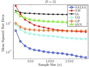
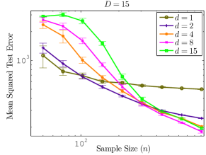
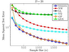
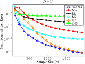
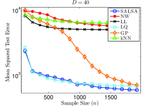
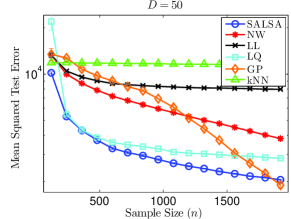
Figure 1: 1 Comparison of SALSA which knows the additive order of $f_{*}$ against other methods. 1 Comparison of different choices of $d$ in SALSA. The best $d$ varies with $n$. 1-1 Comparison of SALSA ($d$ chosen via cross validation) with alternatives on synthetic datasets. In all cases, we plot the mean squared prediction error on a test set of $2000$ points. All curves are produced by averaging over $10$ trials. The error bars are not visible in some curves as they are very small.

4.1 Synthetic Experiments

We begin with a series of synthetic examples. We compare SALSA to some non-additive methods to convey intuition about our additive model. First we create a synthetic low order function of order $d=3$ in $D=15$ dimensions. We do so by creating a $d$ dimensional function $f_{d}$ and add that function over all ${D\choose d}$ combinations of coordinates. We compare SALSA using order $3$ and compare against others. The results are given in Figure 1. This setting is tailored to the assumptions of our method and, not surprisingly, it outperforms all alternatives.

Next we demonstrate the bias variance trade-offs in using additive approximations on non-additive functions. We created a $15$ dimensional (non-additive) function and fitted a SALSA model with $d=1,2,4,8,15$ for difference choices of $n$. The results are given in Figure 1. The interesting observation here is that for small samples sizes small $d$ performs best. However, as we increase the sample size we can also increase the capacity of the model by accommodating higher orders of interaction. In this regime, large $d$ produces the best results. This illustrates our previous point that the order of the additive model gives us another way to control the bias and variance in a regression task. We posit that when $n$ is extremely large, $d=15$ will eventually beat all other models. Finally, we construct synthetic functions in $D=20$ to $50$ dimensions and compare against other methods in Figures 1 to 1. Here, we chose $d$ via cross validation. Our method outperforms or is competitive with other methods.

4.2 Real Datasets

Finally we compare SALSA against the other methods listed above on 16 datasets. The datasets were taken from the UCI repository, Bristol Multilevel Modeling and the following sources: (Tegmark et al, 2006; Wehbe et al., 2014; Just et al., 2010; Guillame-Bert et al., 2014; Tu, 2012; Paschou, 2007). Table 1 gives the average squared error on a test set. For the Speech dataset we have indicated the training time (including cross validation for selecting hyper-parameters) for each method. For SALSA we have also indicated the order $d$ chosen by cross validation. See the caption under the table for more details.

SALSA performs best (or is very close to the best) in 5 of the datasets. Moreover it falls within the top $5$ in all but two datasets, coming sixth in both instances. Observe that in many cases $d$ chosen by SALSA is much smaller than $D$, but importantly also larger than $1$. This observation (along with Fig 1) corroborates a key theme of this paper: while it is true that additive models improve the variance in high dimensional regression, it is often insufficient to confine ourselves to just first order models.

In Appendix D we have given the specifics on the datasets such as preprocessing, the predictors, features etc. We have also discussed some details on the alternatives used.

5 Conclusion

SALSA finds additive approximations to the regression function in high dimensions. It has less bias than first order models and less variance than non-additive methods. Algorithmically, it requires plugging in an additive kernel to KRR. In computing the kernel, we use the Girard-Newton formulae to efficiently sum over a combinatorial number of terms. Our theorems show that the excess risk depends only polynomially on $D$ when $f_{*}$ is additive, significantly better than the usual exponential dependence of nonparametric methods, albeit under stronger assumptions. Our analysis of the agnostic setting provides intuitions on the tradeoffs invovled with changing $d$. We demonstrate the efficacy of SALSA via a comprehensive empirical evaluation. Going forward, we wish to use techniques from scalable kernel methods to handle large datasets.

Theorems 3,4 show polynomial dependence on $D$ when $f_{*}$ is additive. However, these theorems are unsatisfying since in practice regression functions need not be additive. We believe our method did well even on non-additive settings since we could control model capacity via $d$. In this light, we pose the following open problem: identify suitable assumptions to beat existing lower bounds and prove faster convergence of additive models whose additive order $d$ increases with sample size $n$. Our Theorem 5 might be useful in this endeavour.

Acknowledgements

We thank Calvin McCarter, Ryan Tibshirani and Larry Wasserman for the insightful discussions and feedback on the paper. We also thank Madalina Fiterau for providing us with datasets. This work was partly funded by DOE grant DESC0011114.

Dataset ($D$, $n$)	SALSA ($d$)	KRR	kNN	NW	LL	LQ	$\epsilon-$SVR	$\nu-$SVR	GP	RT	GBRT
Housing ($12$, $256$)	$\bf{0.26241}$ (9)	$\underline{0.37690}$	$0.43620$	$0.38431$	$\underline{0.31219}$	0.35061	$1.15272$	$0.38600$	$0.67563$	$1.06015$	$0.42951$
Galaxy ($20$,$2000$)	$\bf{0.00014}$ (4)	$0.01317$	$0.25854$	$0.30615$	$0.01676$	$0.00175$	$0.65280$	$0.15798$	$0.00221$	$0.02293$	$0.01405$
fMRI ($100$,$700$)	$\bf{0.80730}$ (2)	$0.86495$	$0.85645$	$0.84989$	$0.91098$	$1.14079$	$\underline{0.81080}$	$\underline{0.81376}$	$0.84766$	$1.52834$	$0.87326$
Insulin ($50$,$256$)	$\bf{1.02062}$ (3)	$\underline{1.09023}$	$1.15578$	$1.18070$	$\underline{1.06457}$	$1.35747$	$1.10725$	$1.09140$	$1.22404$	$1.58009$	$1.06624$
Skillcraft ($18$,$1700$)	$\bf{0.54695}$ (1)	$\underline{0.54803}$	$0.67155$	$0.73258$	$0.60581$	$1.29690$	$0.71261$	$0.66311$	$\underline{0.54816}$	$1.08047$	$0.57273$
School ($36$,$90$)	$\underline{1.32008}$ (2)	$1.64315$	$\underline{1.37910}$	$\bf{1.14866}$	$2.13390$	$4.79447$	$\underline{1.38173}$	$1.48746$	$1.64215$	$1.99244$	$2.09863$
CCPP* ($59$,$2000$)	$\underline{0.06782}$ (2)	$0.08038$	$0.32017$	$0.33863$	$0.07568$	$\underline{0.06779}$	$0.33707$	$0.094493$	$0.11128$	$1.04527$	$0.06181$
Bleeding ($100$,$200$)	$\underline{0.00123}$ (5)	$0.10633$	$0.16727$	$0.19284$	$\bf{2.48\textrm{e}-6}$	$0.00614$	$0.36505$	$0.03168$	$\underline{6.68\textrm{e}-6}$	$0.18292$	$0.19076$
Speech ($21$, $520$)	$\underline{0.02246}$ (2)	$0.03036$	$0.09348$	$0.11207$	$0.03373$	$\underline{0.02404}$	$\underline{0.22431}$	$0.06994$	$0.02531$	$0.05430$	$0.03515$
Training time	$4.71s$	$0.8s$	$0.18s$	$1.81s$	$4.53s$	$6.80s$	$0.24s$	$27.43s$	$6.34s$	$0.21s$	$5.30s$
Music ($90$,$1000$)	$\underline{0.62512}$ (3)	$\underline{0.61244}$	$0.71141$	$0.75225$	$0.67271$	$1.31957$	$0.75420$	$\bf{0.59399}$	$\underline{0.62429}$	$1.45983$	$0.66652$
Telemonit ($19$, $1000$)	$\underline{0.03473}$ (9)	$0.05640$	$0.09262$	$0.21198$	$0.08253$	$0.18399$	$0.33902$	$0.05246$	$0.03948$	$\bf{0.01375}$	$0.04371$
Propulsion ($15$,$200$)	$\underline{0.00881}$ (8)	$0.05010$	$0.14614$	$0.11237$	$1.12712$	$1.12801$	$0.74511$	$\underline{0.00910}$	$\underline{0.00355}$	$0.02341$	$\bf{0.00061}$
Airfoil* ($40$,$750$)	$\underline{0.51756}$ (5)	$0.53111$	$0.85879$	$0.86752$	$0.51877$	$\underline{0.51105}$	$0.64853$	$0.55118$	$0.54494$	$\underline{0.45249}$	$\bf{0.34461}$
Forestfires($10$, $211$)	$0.35301$ (3)	$\underline{0.28771}$	$0.36571$	$0.37199$	$0.35462$	$12.5727$	$0.70154$	$0.43142$	$\underline{0.29038}$	$0.41531$	$0.26162$
Brain ($29$,$300$)	$0.00036$ (2)	$0.01239$	$0.24429$	$0.22929$	$1.23412$	$2.45781$	$0.27204$	$0.05556$	$\underline{5\textrm{e}-14}$	$0.00796$	$0.00693$
	RBFI	M5’	SI	BF	MARS	COSSO	SpAM	Add-GP	RR	LASSO	LAR
Housing ($12$, $256$)	$0.64871$	$\underline{0.38256}$	$0.50445$	$0.64218$	$0.42379$	$1.30965$	$0.81653$	$0.45656$	$95.60708$	$0.44515$	$0.84410$
Galaxy ($20$,$2000$)	$0.01532$	$\underline{0.00116}$	$0.92189$	$0.94165$	$\underline{0.00163}$	$\underline{0.00153}$	$0.95415$	$-$	$0.13902$	$0.02392$	$1.02315$
fMRI ($100$,$700$)	$1.38585$	$1.42795$	$0.90595$	$0.86197$	$0.90850$	$0.82448$	$0.88014$	$-$	$\underline{0.81005}$	$\underline{0.81390}$	$0.88351$
Insulin ($50$,$256$)	$1.22404$	$1.78252$	$1.20771$	$1.16524$	$1.10359$	$1.13791$	$1.20345$	$-$	$\bf{1.02051}$	$1.11034$	$1.22404$
Skillcraft ($18$,$1700$)	$0.81966$	$1.07195$	$0.87677$	$0.83733$	$\bf{0.54595}$	$\underline{0.55514}$	$0.905445$	$-$	$0.70910$	$0.66496$	$1.00048$
School ($36$,$90$)	$1.61927$	$1.72657$	$1.52374$	$1.48866$	$1.44453$	$1.48046$	$1.59328$	$-$	$1.53416$	$\underline{1.34467}$	$1.64330$
CCPP* ($59$,$2000$)	$1.04257$	$0.10513$	$0.97223$	$0.88084$	$0.08189$	$0.96844$	$\bf{0.06469}$	$-$	$0.07641$	$0.07395$	$1.04527$
Bleeding ($100$,$200$)	$0.13872$	$0.00210$	$0.24918$	$0.37840$	$0.00497$	$0.31362$	$0.41735$	$-$	$\underline{0.00001}$	$\underline{0.00191}$	$0.43488$
Speech ($21$, $520$)	$0.03339$	$0.02843$	$0.39883$	$0.36793$	$\bf{0.01647}$	$0.34863$	$0.66009$	$\underline{0.02310}$	$0.07392$	$0.07303$	$0.73916$
Training time	$0.12s$	$5.70s$	$0.66s$	$27.93s$	$8.11s$	$9.40s$	$76.39s$	$79\,mins$	$0.03s$	$15.94s$	$0.06s$
Music ($90$,$1000$)	$0.78482$	$1.28709$	$0.77347$	$0.75646$	$0.88779$	$0.79816$	$0.76830$	$-$	$0.67777$	$\underline{0.63486}$	$0.78533$
Telemonit ($19$, $1000$)	$\underline{0.02872}$	$\underline{0.01491}$	$0.65386$	$0.84412$	$\underline{0.02400}$	$5.71918$	$0.86425$	$-$	$0.08053$	$0.08629$	$0.94943$
Propulsion ($15$,$200$)	$0.05832$	$0.02341$	$0.27768$	$0.56418$	$0.0129$	$\underline{0.00094}$	$1.11210$	$0.01435$	$0.01490$	$0.02481$	$10.2341$
Airfoil* ($40$,$750$)	$1.00909$	$\underline{0.46714}$	$0.99413$	$0.96668$	$0.54552$	$0.51782$	$0.96231$	$-$	$0.53187$	$0.51986$	$1.00910$
Forestfires($10$, $211$)	$0.45773$	$0.47749$	$0.78057$	$0.88979$	$\underline{0.33891}$	$0.37534$	$0.96944$	$\bf{0.17024}$	$0.47892$	$0.51934$	$1.05415$
Brain ($29$,$300$)	$0.97815$	$\bf{2\textrm{e}-37}$	$0.81711$	$0.63700$	$\underline{5\textrm{e}-31}$	$\underline{2\textrm{e}-6}$	$0.89533$	$-$	$\underline{4\textrm{e}-13}$	$0.00089$	$1.04216$

Table 1: The average squared error on the test set for all methods on 16 datasets. The dimensionality and sample size $n$ are indicated next to the dataset. The best method(s) for each dataset are in bold. The second to fifth methods are underlined. For SALSA we have also indicated the order $d$ chosen by our cross validation procedure in parantheses. The datasets with a * are actually lower dimensional datasets from the UCI repository. But we artificially increase the dimensionality by inserting random values for the remaining coordinates. Even though, this doesn’t change the function value it makes the regression problem harder.

Appendix

Appendix A Proof of Theorem 3: Convergence of SALSA

Our analysis here is a brute force generalisation of the analysis in Zhang et al. (2013). We handle the additive case using ideas from Aronszajn (1950). As such we will try and stick to the same notation. Some intermediate technical results can be obtained directly from Zhang et al. (2013) but we repeat them (or provide an outline) here for the sake of completeness.

In addition to the definitions presented in the main text, we will also need the following quantities,

$$\beta^{(j)}_{t}=\sum_{\ell=t+1}^{\infty}\mu^{(j)}_{\ell},\hskip 14.45377pt\Psi^{(j)}=\sum_{\ell=1}^{\infty}\mu^{(j)}_{\ell},\hskip 14.45377ptb(n,t,q)=\max\left(\sqrt{\max(q,\log t)}\,,\,\frac{\max(q,\log t)}{n^{1/2-1/q}}\right).$$

Here $\Psi^{(j)}$ is the trace of $k^{(j)}$. $\beta^{(j)}_{t}$ depends on some $t\in\mathbb{N}$ which we will pick later. Also define $\beta_{t}=\sum_{j}\beta^{(j)}_{t}$ and $\Psi=\sum_{j}\Psi^{(j)}$.

Note that the excess risk can be decomposed into bias and variance terms, $\mathcal{R}(\hat{f})-\mathcal{R}(f_{*})=\mathbb{E}[\|\hat{f}-f_{*}\|_{2}^{2}]=\|f_{*}-\mathbb{E}\hat{f}\|_{2}^{2}+\mathbb{E}[\|\hat{f}-\mathbb{E}\hat{f}\|_{2}^{2}]$. In Sections A.2 and A.3 respectively, we will prove the following bounds which will yield in Theorem 3:

$$\|f_{*}-\mathbb{E}\hat{f}\|_{2}^{2} \leq M_{d}\Bigg{(}8\lambda\|{\bf f_{*}}\|^{2}_{\mathcal{F}}+\frac{8{M_{d}}^{3/2}\rho^{4}\|{\bf f_{*}}\|^{2}_{\mathcal{F}}}{\lambda}\Psi\beta_{t}+\|{\bf f_{*}}\|^{2}_{\mathcal{F}}\sum_{j=1}^{M_{d}}\mu^{(j)}_{t+1}+\Big{(}\frac{C{M_{d}}b(n,t,q)\rho^{2}\gamma_{k}(\lambda)}{\sqrt{n}}\Big{)}^{q}\|f_{*}\|^{2}_{2}\Bigg{)},$$ (9)

$$\mathbb{E}[\|\hat{f}-\mathbb{E}\hat{f}\|_{2}^{2}] \leq{M_{d}}\Bigg{(}12\lambda\|{\bf f_{*}}\|^{2}_{\mathcal{F}}+\frac{12\sigma^{2}\gamma_{k}(\lambda)}{n}+$$ (10)

$$\hskip 28.90755pt\left(\frac{2\sigma^{2}}{\lambda}+4\|{\bf f_{*}}\|^{2}_{\mathcal{F}}\right)\bigg{(}\sum_{j=1}^{M_{d}}\mu^{(j)}_{t+1}+\frac{12{M_{d}}\rho^{4}}{\lambda}\Psi\beta_{t}+\Big{(}\frac{C{M_{d}}b(n,t,q)\rho^{2}\gamma_{k}(\lambda)}{\sqrt{n}}\Big{)}^{q}\bigg{)}\|f_{*}\|^{2}_{2}\Bigg{)}.$$

Accordingly, this gives the following expression for $\chi(k)$,

$$\chi(k) =\inf_{t}\Bigg{[}\frac{8{M_{d}}^{3/2}\rho^{4}\|{\bf f_{*}}\|^{2}_{\mathcal{F}}}{\lambda}\Psi\beta_{t}+\left(\frac{2\sigma^{2}}{\lambda}+4\|{\bf f_{*}}\|^{2}_{\mathcal{F}}+1\right)\bigg{(}\frac{C{M_{d}}b(n,t,q)\rho^{2}\gamma_{k}(\lambda)}{\sqrt{n}}\bigg{)}^{q}\|f_{*}\|^{2}_{2}\Bigg{)}+$$

$$\hskip 28.90755pt\left(\frac{2\sigma^{2}}{\lambda}+4\|{\bf f_{*}}\|^{2}_{\mathcal{F}}\right)\bigg{(}\sum_{j=1}^{M_{d}}\mu^{(j)}_{t+1}+\frac{12{M_{d}}\rho^{4}}{\lambda}\Psi\beta_{t}\bigg{)}+\|{\bf f_{*}}\|^{2}_{\mathcal{F}}\sum_{j=1}^{M_{d}}\mu^{(j)}_{t+1}\Bigg{]}.$$ (11)

Note that the second term in $\chi(k)$ is usually low order for large enough $q$ due to the $n^{-q/2}$ term. Therefore if in our setting $\beta^{(j)}_{t}$ and $\mu^{(j)}_{t+1}$ are small enough, $\chi(k)$ is low order. We show this for the two kernel choices of Theorem 4 in Appendix B.

First, we review some well known results on RKHS’s which we will use in our analysis. Let $\kappa$ be a PSD kernel and ${\mathcal{H}_{\kappa}}$ be its RKHS. Then $\kappa$ acts as the representer of evaluation – i.e. for any $f\in{\mathcal{H}_{\kappa}}$, $\langle f,\kappa(\cdot,x)\rangle_{\mathcal{H}_{\kappa}}=f(x)$. Denote the RKHS norm $\|f\|_{\mathcal{H}_{\kappa}}=\sqrt{\langle f,f\rangle_{\mathcal{H}_{\kappa}}}$ and the $L^{2}$ norm $\|f\|_{2}=\sqrt{\int f^{2}}$.

Let the kernel $\kappa$ have an eigenexpansion $\kappa(x,x^{\prime})=\sum_{\ell=1}^{\infty}\mu_{\ell}\phi_{\ell}(x)\phi_{\ell}(x^{\prime})$. Denote the basis coefficients of $f$ in $\{\phi_{\ell}\}$ via $\{\theta_{\ell}\}$. That is, $\theta_{\ell}=\int f\cdot\phi_{\ell}\,\mathrm{d}\mathbb{P}$ and $f=\sum_{\ell=1}^{\infty}\theta_{\ell}\phi_{\ell}$. The following results are well known (Schölkopf & Smola, 2001; Steinwart & Christmann, 2008),

$$\langle\phi_{\ell},\phi_{\ell}\rangle=1/\mu_{\ell},\hskip 14.45377pt\|f\|^{2}_{2}=\sum_{\ell=1}^{\infty}\theta_{\ell}^{2},\hskip 14.45377pt\|f\|^{2}_{\mathcal{H}_{\kappa}}=\sum_{\ell=1}^{\infty}\frac{\theta_{\ell}^{2}}{\mu_{\ell}}.$$

Before we proceed, we make the following remark on the minimiser of (3).

Remark 6.

The solution of (3) takes the form $\hat{f}(\cdot)=\sum_{i=1}^{n}\alpha_{i}k(\cdot,X_{i})$ where $k$ is the sum kernel (4).

Proof.

The key observation is that we only need to consider $n$ (and not $n{M_{d}}$) parameters even though we are optimising over ${M_{d}}$ RKHSs. The reasoning uses a powerful result from Aronszajn (1950). Consider the class of functions $\mathcal{H}^{\prime}=\{f=\sum_{j}f^{(j)};f^{(j)}\in{{\mathcal{H}_{k^{(j)}}}}\}$. In (3) we are minimising over $\mathcal{H}^{\prime}$. Any $f\in\mathcal{H}^{\prime}$ need not have a unique additive decomposition. Consider $\mathcal{H}\subset\mathcal{H}^{\prime}$ which only contains the minimisers in the expression below.

$$\|f\|^{2}_{\mathcal{H}}=\inf_{g^{(j)}\in{{\mathcal{H}_{k^{(j)}}}};f=\sum g^{(j)}}\sum_{j=1}^{M}\|g^{(j)}\|^{2}_{{\mathcal{H}_{k^{(j)}}}}$$

Aronszajn (1950) showed that $\mathcal{H}$ is an RKHS with the sum kernel $k=\sum_{j}k^{(j)}$ and its RKHS norm is $\|\cdot\|_{\mathcal{H}}$. Clearly, the minimiser of (3) lies in $\mathcal{H}$. For any $g^{\prime}\in\mathcal{H}^{\prime}$, we can pick a corresponding $g\in\mathcal{H}$ with the same sum of squared errors (as $g=g^{\prime}$) but lower complexity penalty (as $g$ minimises the sum of norms for any $g^{\prime}=g$). Therefore, we may optimise (3) just over $\mathcal{H}$ and not $\mathcal{H}^{\prime}$. An application of Mercer’s theorem concludes the proof. ∎

A.1 Set up

We first define the following function class of the product of all RKHS’s, $\mathcal{F}={\mathcal{H}_{k^{(1)}}}\times{\mathcal{H}_{k^{(2)}}}\times\dots\times{\mathcal{H}_{k^{({M_{d}})}}}=\left\{{\bf f}=(f^{(1)},\dots,f^{({M_{d}})})\big{|}f^{(j)}\in{{\mathcal{H}_{k^{(j)}}}}\;\forall j\right\}$ and equip it with the inner product $\left\langle{\bf f}_{1},{\bf f}_{2}\right\rangle=\langle f^{(1)}_{1},f^{(1)}_{2}\rangle_{{\mathcal{H}_{k^{(1)}}}}+\dots+\langle f^{({M_{d}})}_{1},f^{({M_{d}})}_{2}\rangle_{{\mathcal{H}_{k^{(M_{d})}}}}.$ Here, $f^{(j)}_{1}$ are the elements of ${\bf f}_{1}$ and $\langle\cdot,\cdot\rangle_{{{\mathcal{H}_{k^{(j)}}}}}$ is the RKHS inner product of ${{\mathcal{H}_{k^{(j)}}}}$. Therefore the norm is $\|{\bf f}\|_{\mathcal{F}}^{2}=\sum_{j=1}^{M_{d}}\|f^{(j)}\|^{2}_{{\mathcal{H}_{k^{(j)}}}}$. Denote $\xi^{(j)}_{x}=k^{(j)}(x,\cdot)$ and $\xi_{x}(\cdot)=\mathcal{K}(\cdot,x)$. Observe that for an additive function $f=\sum_{j}f^{(j)}(x)$,

$$f(x)=\sum_{j}f^{(j)}(x)=\sum_{j}\langle f^{(j)},\xi^{(j)}_{x}\rangle_{{\mathcal{H}_{k^{(j)}}}}=\langle{\bf f},\xi_{x}\rangle.$$

Recall that the solution to (3) is denoted by $\hat{f}$ and the individual functions of the solution are given by $\hat{f}^{(j)}$. We will also use ${\bf f_{*}}$ and ${\bf\hat{f}}$ to denote the representations of $f_{*}$ and $\hat{f}$ in $\mathcal{F}$, i.e., ${\bf f_{*}}=(f_{*}^{(1)},\dots,f_{*}^{({M_{d}})})$ and ${\bf\hat{f}}=(\hat{f}^{(1)},\dots,\hat{f}^{({M_{d}})})$. Note that $\|{\bf f_{*}}\|^{2}_{\mathcal{F}}$ is precisely the bound used in Theorem 3. We will also denote $\Delta^{(j)}=\hat{f}^{(j)}-f_{*}^{(j)}\in{{\mathcal{H}_{k^{(j)}}}}$, $\bm{\Delta}=(\Delta^{(1)},\dots,\Delta^{({M_{d}})})\in\mathcal{F}$, and $\Delta=\sum_{j}\Delta^{(j)}=\hat{f}-f_{*}$.

For brevity, from now on we will write $k^{(j)}(x,x^{\prime})$ instead of $k^{(j)}(x^{(j)},{x^{(j)}}^{\prime})$. Further, since $d$ is fixed in this analysis we will write $M$ for ${M_{d}}$.

A.2 Bias (Proof of Bound (9))

Note that we need to bound $\|\mathbb{E}[\Delta]\|_{2}$ which by Jensen’s inequality is less than $\mathbb{E}[\|\mathbb{E}[\Delta|X_{1}^{n}]\|_{2}]$. Since, $\|\mathbb{E}[\Delta|X_{1}^{n}]\|_{2}^{2}\leq M\sum_{j=1}^{M}\|\mathbb{E}[\Delta^{(j)}|X_{1}^{n}]\|_{2}^{2}$, we will focus on bounding $\sum_{j=1}^{M}\|\mathbb{E}[\Delta^{(j)}|X_{1}^{n}]\|_{2}^{2}$.

We can write the optimisation objective (3) as follows,

$${\bf\hat{f}}=\mathop{\mathrm{argmin}}_{{\bf f}\in\mathcal{F}}\frac{1}{n}\sum_{i=1}^{n}\left(\langle{\bf f},\xi_{X_{i}}\rangle-Y_{i}\right)^{2}+\lambda\|{\bf f}\|^{2}_{\mathcal{F}}$$ (12)

Since this is Fréchet differentiable in $\mathcal{F}$ in the metric induced by the inner product defined above, the first order optimality conditions for $\hat{f}^{(j)}$ give us,

$$\frac{1}{n}\sum_{i=1}^{n}\left(\langle\xi_{X_{i}},{\bf\hat{f}}-{\bf f_{*}}\rangle-\epsilon_{i}\right)\xi^{(j)}_{X_{i}}\;+\;2\lambda\hat{f}^{(j)}={\bf 0}.$$

Here, we have taken $Y_{i}=f_{*}(X_{i})+\epsilon_{i}$ where $\mathbb{E}[\epsilon_{i}|X_{i}]=0$. Doing this for all $\hat{f}^{(j)}$ we have,

$$\frac{1}{n}\sum_{i=1}^{n}\xi_{X_{i}}\left(\langle\xi_{X_{i}},\bm{\Delta}\rangle-\epsilon_{i}\right)+\lambda{\bf\hat{f}}={\bf 0}$$ (13)

Taking expectations conditioned on $X_{1}^{n}$ and rearranging we get,

$$(\widehat{\Sigma}+\lambda I)\mathbb{E}[\bm{\Delta}|X_{1}^{n}]=-\lambda{\bf f_{*}},$$ (14)

where $\widehat{\Sigma}=\frac{1}{n}\sum_{i}\xi_{X_{i}}\otimes\xi_{X_{i}}$ is the empirical covariance. Since $\widehat{\Sigma}\succeq{\bf 0}$,

$$\forall j^{\prime},\;\;\;\|\mathbb{E}[\Delta^{(j^{\prime})}|X_{1}^{n}]\|^{2}_{{\mathcal{H}_{k^{(j^{\prime})}}}}\leq\sum_{j=1}^{M}\|\mathbb{E}[\Delta^{(j)}|X_{1}^{n}]\|_{{\mathcal{H}_{k^{(j)}}}}^{2}=\|\mathbb{E}[\bm{\Delta}|X_{1}^{n}]\|^{2}_{\mathcal{F}}\leq\|{\bf f_{*}}\|^{2}_{\mathcal{F}}$$ (15)

Let $\mathbb{E}[\Delta^{(j)}|X_{1}^{n}]=\sum_{\ell=1}^{\infty}\delta^{(j)}_{\ell}\phi^{(j)}_{\ell}$ where $\phi^{(j)}_{\ell}$ are the eigenfunctions in the expansion of $k^{(j)}$. Denote $\delta^{(j)}_{\downarrow}=(\delta^{(j)}_{1},\dots,\delta^{(j)}_{t})$ and $\delta^{(j)}_{\uparrow}=(\delta^{(j)}_{t+1},\delta^{(j)}_{t+2},\dots)$. We will set $t$ later. Since $\|\mathbb{E}[\Delta^{(j)}|X_{1}^{n}]\|_{2}^{2}=\|\delta^{(j)}_{\downarrow}\|_{2}^{2}+\|\delta^{(j)}_{\uparrow}\|_{2}^{2}$ we will bound the two terms. The latter term is straightforward,

$$\|\delta^{(j)}_{\uparrow}\|_{2}^{2}\leq\mu^{(j)}_{t+1}\sum_{\ell=t+1}^{\infty}\frac{{\delta^{(j)}_{\ell}}^{2}}{\mu^{(j)}_{\ell}}\leq\mu^{(j)}_{t+1}\|\mathbb{E}[\Delta^{(j)}|X_{1}^{n}]\|^{2}_{{\mathcal{H}_{k^{(j)}}}}\leq\mu^{(j)}_{t+1}\|{\bf f_{*}}\|^{2}_{\mathcal{F}}$$ (16)

To control $\|\delta^{(j)}_{\downarrow}\|$, let $f_{*}^{(j)}=\sum_{\ell}\theta^{(j)}_{\ell}\phi^{(j)}_{\ell}$. Also, define the following: $\theta^{(j)}_{\downarrow}=(\theta^{(j)}_{1},\dots,\theta^{(j)}_{t})$, $\Phi^{(j)}\in\mathbb{R}^{n\times t}$, $\Phi^{(j)}_{i\ell}=\phi^{(j)}_{\ell}(X_{i})$, $\Phi^{(j)}_{\ell}=(\phi^{(j)}_{\ell}(X_{1}),\dots,\phi^{(j)}_{\ell}(X_{n}))\in\mathbb{R}^{n}$, $\mathcal{M}^{(j)}={\rm diag}(\mu^{(j)}_{1},\dots,\mu^{(j)}_{t})\in\mathbb{R}_{+}^{t\times t}$ and $v^{(j)}\in\mathbb{R}^{n}$ where $v^{(j)}_{i}=\sum_{\ell>t}\delta^{(j)}_{\ell}\phi^{(j)}_{\ell}(X_{i})=\mathbb{E}[\Delta^{(j)}_{\uparrow}(X_{i})|X_{1}^{n}]$.

Further define, $\Phi=[\Phi^{(1)}\dots\Phi^{(M)}]\in\mathbb{R}^{n\times tM}$, $\mathcal{M}={\rm diag}(\mathcal{M}^{(1)},\dots,\mathcal{M}^{(M)})\in\mathbb{R}^{tM\times tM}$, $v_{i}=\sum_{j}v^{(j)}$, $\delta_{\downarrow}=[\delta^{(1)}_{\downarrow};\dots;\delta^{(M)}_{\downarrow}]\in\mathbb{R}^{tM}$ and $\theta_{\downarrow}=[\theta^{(1)}_{\downarrow};\dots;\theta^{(M)}_{\downarrow}]\in\mathbb{R}^{tM}$.

Now compute the $\mathcal{F}$-inner product between $({\bf 0},\dots,\phi^{(j)}_{\ell},\dots,{\bf 0})$ with equation (14) to obtain,

$$\frac{1}{n}\sum_{i=1}^{n}\langle\phi^{(j)}_{\ell},\xi^{(j)}_{X_{i}}\rangle_{{\mathcal{H}_{k^{(j)}}}}\langle\xi_{X_{i}},\mathbb{E}[\bm{\Delta}|X_{1}^{n}]\rangle+\lambda\langle\phi^{(j)}_{\ell},\mathbb{E}[\Delta^{(j)}|X_{1}^{n}]\rangle_{{\mathcal{H}_{k^{(j)}}}} =-\lambda\langle\phi^{(j)}_{\ell},f_{*}^{(j)}\rangle_{{\mathcal{H}_{k^{(j)}}}}$$

$$\frac{1}{n}\sum_{i=1}^{n}\phi^{(j)}_{\ell}(X_{i})\sum_{j=1}^{M}\left(\sum_{\ell^{\prime}\leq t}\phi^{(j)}_{\ell^{\prime}}(X_{i})\delta^{(j)}_{\ell^{\prime}}+\sum_{\ell^{\prime}>t}\phi^{(j)}_{\ell^{\prime}}(X_{i})\delta^{(j)}_{\ell^{\prime}}\right)+\lambda\frac{\delta^{(j)}_{\ell}}{\mu^{(j)}_{\ell}} =-\lambda\frac{\theta^{(j)}_{\ell}}{\mu^{(j)}_{\ell}}$$

After repeating this for all $j$ and for all $\ell=1,\dots,t$, and arranging the terms appropriately this reduces to

$$\left(\frac{1}{n}\Phi^{\top}\Phi+\lambda\mathcal{M}^{-1}\right)\delta_{\downarrow}=-\lambda\mathcal{M}^{-1}\theta_{\downarrow}-\frac{1}{n}\Phi^{\top}v$$

By writing $Q=(I+\lambda\mathcal{M}^{-1})^{1/2}$, we can rewrite the above expression as

$$\left(I+Q^{-1}\left(\frac{1}{n}\Phi^{\top}\Phi-I\right)Q^{-1}\right)Q\delta_{\downarrow}=-\lambda Q^{-1}\mathcal{M}^{-1}\theta_{\downarrow}-\frac{1}{n}Q^{-1}\Phi^{\top}v.$$

We will need the following technical lemmas. The proofs are given at the end of this section. These results correspond to Lemma 5 in Zhang et al. (2013).

Lemma 7.

$\|\lambda Q^{-1}\mathcal{M}^{-1}\theta_{\downarrow}\|_{2}^{2}\leq\lambda\|{\bf f_{*}}\|^{2}_{\mathcal{F}}$.

Lemma 8.

$\mathbb{E}\left[\|\frac{1}{n}Q^{-1}\Phi^{\top}v\|_{2}^{2}\right]\leq\frac{1}{\lambda}M^{3/2}\rho^{4}\|{\bf f_{*}}\|^{2}_{\mathcal{F}}\Psi\beta_{t}$.

Lemma 9.

Define the event $\mathcal{E}=\{\|Q^{-1}(\frac{1}{n}\Phi^{\top}\Phi-I)Q^{-1}\|_{op}\leq 1/2\}$. Then, there exists a constant $C$ s.t.

$$\mathbb{P}(\mathcal{E}^{c})\leq\left(\max\left(\sqrt{\max(q,\log t)}\;,\;\frac{\max(q,\log t)}{n^{1/2-1/q}}\right)\times\frac{MC\rho^{2}\gamma_{k}(\lambda)}{\sqrt{n}}\right)^{q}.$$

When $\mathcal{E}$ holds, by Lemma 9 and noting that $Q\succeq I$,

$$\|\delta_{\downarrow}\|^{2}_{2}\leq\|Q\delta_{\downarrow}\|_{2}^{2} =\Big{\|}\left(I+Q^{-1}\left(\frac{1}{n}\Phi^{\top}\Phi-I\right)Q^{-1}\right)^{-1}\left(-\lambda Q^{-1}\mathcal{M}^{-1}\theta_{\downarrow}-\frac{1}{n}Q^{-1}\Phi^{\top}v\right)\Big{\|}^{2}$$

$$\leq 4\|\lambda Q^{-1}\mathcal{M}^{-1}\theta_{\downarrow}+\frac{1}{n}Q^{-1}\Phi^{\top}v\|_{2}^{2}.\leq 8\|\lambda Q^{-1}\mathcal{M}^{-1}\theta_{\downarrow}\|_{2}^{2}+8\|\frac{1}{n}Q^{-1}\Phi^{\top}v\|_{2}^{2}$$

Now using Lemmas 7 and 8,

$$\mathbb{E}[\|\delta_{\downarrow}\|_{2}^{2}|\mathcal{E}]\leq 8\left(\lambda\|{\bf f_{*}}\|^{2}_{\mathcal{F}}+\frac{M^{3/2}\rho^{4}\|{\bf f_{*}}\|^{2}_{\mathcal{F}}\Psi\beta_{t}}{\lambda}\right)$$

Since $\mathbb{E}[\|\delta_{\downarrow}\|_{2}^{2}]=\mathbb{P}(\mathcal{E})\mathbb{E}[\|\delta_{\downarrow}\|_{2}^{2}|\mathcal{E}]+\mathbb{P}(\mathcal{E}^{c})\mathbb{E}[\|\delta_{\downarrow}\|_{2}^{2}|\mathcal{E}^{c}]$ and by using the fact that $\|\delta_{\downarrow}\|^{2}\leq\|\mathbb{E}[\Delta|X_{1}^{n}]\|_{2}^{2}\leq\|f_{*}\|^{2}_{2}$, we have

$$\mathbb{E}[\|\delta_{\downarrow}\|_{2}^{2}] \leq 8\lambda\|{\bf f_{*}}\|^{2}_{\mathcal{F}}+\frac{8M\rho^{4}\|{\bf f_{*}}\|^{2}_{\mathcal{F}}\Psi\beta_{t}}{\lambda}\;+$$

$$\hskip 21.68121pt\left(\max\left(\sqrt{\max(q,\log t)}\;,\;\frac{\max(q,\log t)}{n^{1/2-1/q}}\right)\times\frac{MC\rho^{2}\gamma_{k}(\lambda)}{\sqrt{n}}\right)^{q}\|f_{*}\|^{2}_{2}$$

Finally using (16) and by noting that

$$\|\mathbb{E}[\Delta|X_{1}^{n}]\|_{2}^{2}\;\;\leq M\sum_{j=1}^{M}\|\mathbb{E}[\Delta^{(j)}|X_{1}^{n}]\|_{2}^{2}\;\;=M\big{(}\|\delta_{\downarrow}\|_{2}^{2}+\sum_{j}\|\delta^{(j)}_{\uparrow}\|_{2}^{2}\big{)}\;\;\leq M\big{(}\|\delta_{\downarrow}\|_{2}^{2}+\|{\bf f_{*}}\|^{2}_{\mathcal{F}}\sum_{j}\mu^{(j)}_{t+1}\big{)}$$

and then taking expectation over $X_{1}^{n}$, we obtain the bound for the bias in (9).

Proofs of Technical Lemmas

A.2.1 Proof of Lemma 7

Lemma 7 is straightforward.

$$\|Q^{-1}\mathcal{M}^{-1}\theta_{\downarrow}\|_{2}^{2} =\sum_{j=1}^{M}\|{Q^{(j)}}^{-1}{\mathcal{M}^{(j)}}^{-1}\theta^{(j)}_{\downarrow}\|_{2}^{2}=\sum_{j=1}^{M}{\theta^{(j)}_{\downarrow}}^{\top}({\mathcal{M}^{(j)}}^{2}+\lambda{\mathcal{M}^{(j)}})^{-1}\theta^{(j)}_{\downarrow}$$

$$\leq\sum_{j=1}^{M}{\theta^{(j)}_{\downarrow}}^{\top}(\lambda{\mathcal{M}^{(j)}})^{-1}\theta^{(j)}_{\downarrow}=\frac{1}{\lambda}\sum_{j=1}^{M}\sum_{\ell=1}^{t}\frac{{\theta^{(j)}_{\ell}}^{2}}{\mu^{(j)}_{\ell}}\leq\frac{1}{\lambda}\|{\bf f_{*}}\|^{2}_{\mathcal{F}}$$

A.2.2 Proof of Lemma 8

We first decompose the LHS as follows,

$$\left\|\frac{1}{n}Q^{-1}\Phi^{\top}v\right\|_{2}^{2}=\left\|(M+\lambda I)^{-1/2}\left(\frac{1}{n}M^{1/2}\Phi^{\top}v\right)\right\|_{2}^{2}\leq\frac{1}{\lambda}\left\|\frac{1}{n}M^{1/2}\Phi^{\top}v\right\|_{2}^{2}$$ (17)

The last step follows by noting that $\|(M+\lambda I)^{-1/2}\|^{2}_{op}=\max_{j,\ell}1/(\mu^{(j)}_{\ell}+\lambda)\leq 1/\lambda$. Further,

$$\mathbb{E}\left[\|M^{1/2}\Phi^{\top}v\|_{2}^{2}\right]=\sum_{j=1}^{M}\sum_{\ell=1}^{t}\mu^{(j)}_{\ell}\mathbb{E}[({\Phi^{(j)}_{\ell}}^{\top}v)^{2}]\leq\sum_{j=1}^{M}\sum_{\ell=1}^{t}\mu^{(j)}_{\ell}\mathbb{E}[\|\Phi^{(j)}_{\ell}\|_{2}^{2}\|v\|_{2}^{2}]$$ (18)

Note that the term inside the summation in the RHS can be bounded by, $\sqrt{\mathbb{E}[\|\Phi^{(j)}_{\ell}\|^{4}_{2}]\mathbb{E}[\|v\|^{4}_{2}]}$. We bound the first expectation via,

$$\mathbb{E}\left[\|\Phi^{(j)}_{\ell}\|^{4}\right]=\mathbb{E}\left[\bigg{(}\sum_{i=1}^{n}\phi^{(j)}_{\ell}(X_{i})^{2}\bigg{)}^{2}\right]\leq\mathbb{E}\left[n\sum_{i=1}^{n}\phi^{(j)}_{\ell}(X_{i})^{4}\right]\leq n^{2}\rho^{4}$$

where the last step follows from Assumption 2. For the second expectation we first bound $\|v\|^{4}$,

$$\|v\|_{2}^{4}=\left(\sum_{i=1}^{n}\bigg{(}\sum_{j=1}^{M}v^{(j)}_{i}\bigg{)}^{2}\right)^{2}\leq\left(M\sum_{i=1}^{n}\sum_{j=1}^{M}{v^{(j)}_{i}}^{2}\right)^{2}\leq M^{3}n\sum_{i=1}^{n}\sum_{j=1}^{M}{v^{(j)}_{i}}^{4}$$

Now by the Cauchy Schwarz inequality,

$${v^{(j)}_{i}}^{2}=\bigg{(}\sum_{\ell>t}\delta^{(j)}_{\ell}\phi^{(j)}_{\ell}(X_{i})\bigg{)}^{2}\leq\bigg{(}\sum_{\ell>t}\frac{{\delta^{(j)}_{\ell}}^{2}}{\mu^{(j)}_{\ell}}\bigg{)}\bigg{(}\sum_{\ell>t}\mu^{(j)}_{\ell}\phi^{(j)}_{\ell}(X_{i})^{2}\bigg{)}.$$

Therefore,

$$\mathbb{E}\left[\|v\|^{4}\right] \leq M^{3}n\sum_{i=1}^{n}\sum_{j=1}^{M}\mathbb{E}\left[\|\mathbb{E}[\Delta^{(j)}|X_{1}^{n}]\|_{{\mathcal{H}_{k^{(j)}}}}^{4}\bigg{(}\sum_{\ell>t}\mu^{(j)}_{\ell}\phi^{(j)}_{\ell}(X_{i})^{2}\bigg{)}^{2}\right]$$

$$\leq M^{3}n\|{\bf f_{*}}\|_{\mathcal{F}}^{4}\sum_{j=1}^{M}\sum_{i=1}^{n}\sum_{\ell,\ell^{\prime}>t}\mathbb{E}[\mu^{(j)}_{\ell}\mu^{(j)}_{\ell^{\prime}}\phi^{(j)}_{\ell}(X_{i})^{2}\phi^{(j)}_{\ell^{\prime}}(X_{i})^{2}]$$

$$\leq M^{3}n\rho^{4}\|{\bf f_{*}}\|_{\mathcal{F}}^{4}\sum_{j=1}^{M}\sum_{i=1}^{n}\left(\sum_{\ell>t}\mu^{(j)}_{\ell}\right)^{2}\leq M^{3}n^{2}\rho^{4}\|{\bf f_{*}}\|_{\mathcal{F}}^{4}\sum_{j=1}^{M}{\beta^{(j)}_{t}}^{2}$$

Here, in the first step we have used the definition of $\|\mathbb{E}[\Delta^{(j)}|X_{1}^{n}]\|_{{\mathcal{H}_{k^{(j)}}}}$, in the second step, equation (15), in the third step assumption 2 and Cauchy Schwarz, and in the last step, the definition of $\beta_{t}$. Plugging this back into (18), we get

$$\mathbb{E}\left[\|M^{1/2}\Phi^{\top}v\|^{2}\right]\leq M^{3/2}n^{2}\rho^{4}\|{\bf f_{*}}\|^{2}_{\mathcal{F}}\sqrt{\sum_{j=1}^{M}{\beta^{(j)}_{t}}^{2}}\sum_{j=1}^{M}\sum_{\ell=1}^{t}\mu^{(j)}_{\ell}\leq M^{3/2}n^{2}\rho^{4}\|{\bf f_{*}}\|^{2}_{\mathcal{F}}\Psi\beta_{t}$$

This bound, along with equation (17) gives us the desired result.

A.2.3 Proof of Lemma 9

Define $\pi^{(j)}_{i}=\{\phi^{(j)}_{\ell}(x_{i})\}_{\ell=1}^{t}\in\mathbb{R}^{t}$, $\pi_{i}=[\pi^{(1)}_{i};\dots;\pi^{(M)}_{i}]\in\mathbb{R}^{tM}$ and the matrices $A_{i}=Q^{-1}(\pi_{i}\pi_{i}^{\top}-I)Q^{-1}\in\mathbb{R}^{tm\times tM}$. Note that $A_{i}=A_{i}^{\top}$ and

$$\mathbb{E}[A_{i}]=Q^{-1}(\mathbb{E}[\pi_{i}\pi_{i}^{\top}]-I)Q^{-1}={\bf 0}.$$

Then, if $\epsilon_{i},i=1,\dots,n$ are i.i.d Rademacher random variables, by a symmetrization argument we have,

$$\mathbb{E}\left[\Big{\|}Q^{-1}\left(\frac{1}{n}\Phi^{\top}\Phi-I\right)Q^{-1}\Big{\|}_{op}^{k}\right]=\mathbb{E}\left[\Big{\|}\frac{1}{n}\sum_{i=1}^{n}A_{i}\Big{\|}_{op}^{k}\right]\leq 2^{k}\mathbb{E}\left[\Big{\|}\frac{1}{n}\sum_{i=1}^{n}\epsilon_{i}A_{i}\Big{\|}_{op}^{k}\right]$$ (19)

The above term can be bounded by the following expression.

$$2^{q}\left(\sqrt{e\max(q,\log(t))}\frac{\rho^{2}\sqrt{M}}{\sqrt{n}}\sqrt{\sum_{\ell=1}^{M}\gamma^{(j)}(\lambda)^{2}}+4e\max(q,\log(t))\rho^{2}\left(\frac{M}{n}\right)^{1-1/q}\left(\sum_{\ell=1}^{M}\gamma^{(j)}(\lambda)^{q}\right)^{1/q}\right)^{q}$$

$$\leq\left(\frac{C}{2}\right)^{q}\max\left(\sqrt{M(\max(q,\log t))},\frac{M^{1-1/q}\max(q,\log t)}{n^{1/2-1/q}}\right)^{q}\left(\frac{\rho^{2}\gamma_{k}(\lambda)}{\sqrt{n}}\right)^{q}$$

The proof mimics Lemma 6 in (Zhang et al., 2013) by performing essentially the same steps over $\mathcal{F}$ instead of the usual Hilbert space. In many of the steps, $M$ terms appear (instead of the one term for KRR) which is accounted for via Jensen’s inequality.

Finally, by Markov’s inequality,

$$\mathbb{P}(\mathcal{E}^{c}) \leq 2^{k}\mathbb{E}\left[\Big{\|}Q^{-1}\left(\frac{1}{n}\Phi^{\top}\Phi-I\right)Q^{-1}\Big{\|}_{op}^{q}\right]$$

$$\leq C^{q}\max\left(\sqrt{M(\max(q,\log t))},\frac{M^{1-1/q}\max(q,\log t)}{n^{1/2-1/q}}\right)^{q}\left(\frac{\rho^{2}\gamma_{k}(\lambda)}{\sqrt{n}}\right)^{q}$$

A.3 Variance (Proof of Bound (10))

Once again, we follow Zhang et al. (2013). The tricks we use to generalise it to the additive case (i.e. over $\mathcal{F}$) are the same as that for the bias. Note that since $\mathbb{E}[\|\hat{f}-\mathbb{E}\hat{f}\|_{2}^{2}]\leq\mathbb{E}[\|\hat{f}-g\|_{2}^{2}]$ for all $g$, it is sufficient to bound $\mathbb{E}[\|\hat{f}-f_{*}\|_{2}^{2}]=\mathbb{E}[\|\Delta\|_{2}^{2}]$.

First note that,

$$\lambda\mathbb{E}[\|{\bf\hat{f}}\|^{2}_{\mathcal{F}}|X_{1}^{n}]\;\;\leq\mathbb{E}\left[\frac{1}{n}\sum_{i=1}^{n}\left(\hat{f}(X_{i})-Y_{i}\right)^{2}+\lambda\|{\bf\hat{f}}\|^{2}_{\mathcal{F}}\bigg{|}X_{1}^{n}\right]\;\;\leq\frac{1}{n}\sum_{i=1}^{n}\mathbb{E}[\epsilon_{i}^{2}|X_{1}^{n}]+\lambda\|{\bf f_{*}}\|^{2}_{\mathcal{F}}\leq\sigma^{2}+\lambda\|{\bf f_{*}}\|^{2}_{\mathcal{F}}$$

The second step follows by the fact that ${\bf\hat{f}}$ is the minimiser of (12). Then, for all $j$,

$$\mathbb{E}[\|\Delta^{(j)}\|_{{\mathcal{H}_{k^{(j)}}}}^{2}|X_{1}^{n}]\leq\mathbb{E}[\|\bm{\Delta}\|^{2}_{\mathcal{F}}|X_{1}^{n}]\leq 2\|{\bf f_{*}}\|^{2}_{\mathcal{F}}+2\mathbb{E}[\|{\bf\hat{f}}\|_{2}^{2}|X_{1}^{n}]\leq\frac{2\sigma^{2}}{\lambda}+4\|{\bf f_{*}}\|^{2}_{\mathcal{F}}$$ (20)

Let $\Delta^{(j)}=\sum_{\ell=1}^{\infty}\delta^{(j)}_{\ell}\phi^{(j)}_{\ell}$. Note that the definition of $\delta^{(j)}_{\ell}$ is different here. Define $\delta^{(j)}_{\downarrow},\delta^{(j)}_{\uparrow},\Delta^{(j)}_{\downarrow},\Delta^{(j)}_{\uparrow},\delta_{\downarrow}$ analogous to the definitions in Section A.2. Then similar to before we have,

$$\mathbb{E}[\|\delta^{(j)}_{\uparrow}\|_{2}^{2}]\leq\mu^{(j)}_{t+1}\mathbb{E}[\|\Delta^{(j)}_{\uparrow}\|^{2}_{{\mathcal{H}_{k^{(j)}}}}]\leq\mu^{(j)}_{t+1}\left(\frac{2\sigma^{2}}{\lambda}+4\|{\bf f_{*}}\|^{2}_{\mathcal{F}}\right)$$

We may use this to obtain a bound on $\mathbb{E}[\|\Delta_{\uparrow}\|^{2}]$. To obtain a bound on $\mathbb{E}[\|\Delta_{\downarrow}\|^{2}]$, take the $\mathcal{F}$ inner product of $({\bf 0},\dots,\phi^{(j)}_{\ell},\dots,{\bf 0})$ with the first order optimality condition (13) and following essentially the same procedure to the bias we get,

$$\left(\frac{1}{n}\Phi^{\top}\Phi+\lambda\mathcal{M}^{-1}\right)\delta_{\downarrow}=-\lambda\mathcal{M}^{-1}\theta_{\downarrow}-\frac{1}{n}\Phi^{\top}v+\frac{1}{n}\Phi^{\top}\epsilon$$

where $\Phi,\mathcal{M},\theta_{\downarrow}$ are the same as in the bias calculation. $v^{(j)}\in\mathbb{R}^{n}$ where $v^{(j)}_{i}=\sum_{\ell>t}\delta^{(j)}_{\ell}\phi^{(j)}_{\ell}(X_{i})=\mathbb{E}[\Delta^{(j)}_{\uparrow}(X_{i})|X_{1}^{n}]$ (recall that $\delta^{(j)}_{\ell}$ is different to the definition in the bias) and $\epsilon\in\mathbb{R}^{n}$, $\epsilon_{i}=Y_{i}-f_{*}(X_{i})$ is the vector of errors. Then we write,

$$\left(I+Q^{-1}\left(\frac{1}{n}\Phi^{\top}\Phi-I\right)Q^{-1}\right)Q\delta_{\downarrow}=-\lambda Q^{-1}\mathcal{M}^{-1}\theta_{\downarrow}-\frac{1}{n}Q^{-1}\Phi^{\top}v+\frac{1}{n}Q^{-1}\Phi^{\top}\epsilon$$

where $Q=(I+\lambda\mathcal{M}^{-1})^{1/2}$ as before. Following a similar argument to the bias, when the event $\mathcal{E}$ holds,

$$\|\delta_{\downarrow}\|_{2}^{2}\leq\|Q\delta_{\downarrow}\|_{2}^{2} \leq 4\|\lambda Q^{-1}\mathcal{M}^{-1}\theta_{\downarrow}+\frac{1}{n}Q^{-1}\Phi^{\top}v+\frac{1}{n}Q^{-1}\Phi^{\top}\epsilon\|_{2}^{2}$$

$$\leq 12\|\lambda Q^{-1}\mathcal{M}^{-1}\theta_{\downarrow}\|^{2}+12\|\frac{1}{n}Q^{-1}\Phi^{\top}v\|^{2}+12\|\frac{1}{n}Q^{-1}\Phi^{\top}\epsilon\|_{2}^{2}$$ (21)

By Lemma 7, the first term can be bounded via $12\lambda\|{\bf f_{*}}\|^{2}_{\mathcal{F}}$. For the second and third terms we use the following two lemmas, the proofs of which are given at the end of this subsection.

Lemma 10.

$\mathbb{E}\left[\|\frac{1}{n}Q^{-1}\Phi^{\top}v\|_{2}^{2}\right]\leq\frac{1}{\lambda}M\rho^{4}\Psi\beta_{t}(2\sigma^{2}/\lambda+4\|{\bf f_{*}}\|^{2}_{\mathcal{F}})$.

Lemma 11.

$\mathbb{E}\left[\big{\|}\frac{1}{n}Q^{-1}\Phi^{\top}\epsilon\big{\|}_{2}^{2}\right]\leq\frac{\sigma^{2}}{n}\gamma_{k}(\lambda)$

Note that $\mathbb{E}[\|\delta_{\downarrow}\|^{2}_{2}]\leq\mathbb{P}(\mathcal{E})\mathbb{E}[\|\delta_{\downarrow}\|_{2}^{2}|\mathcal{E}]+\mathbb{E}[\mathbbm{1}(\mathcal{E}^{c})\|\delta_{\downarrow}\|_{2}^{2}]$. The bound on the first term comes via equation (21) and Lemmas 7, 10 and 11. The second term can be bound via,

$$\mathbb{E}[\mathbbm{1}(\mathcal{E}^{c})\|\delta_{\downarrow}\|_{2}^{2}] \leq\mathbb{E}[\mathbbm{1}(\mathcal{E}^{c})\mathbb{E}[\|\bm{\Delta}\|_{\mathcal{F}}^{2}|X_{1}^{n}]$$

$$\leq\left(\max\left(\sqrt{\max(q,\log t)}\;,\;\frac{\max(q,\log t)}{n^{1/2-1/q}}\right)\times\frac{MC\rho^{2}\gamma_{k}(\lambda)}{\sqrt{n}}\right)^{q}\left(\frac{2\sigma^{2}}{\lambda}+4\|{\bf f_{*}}\|^{2}_{\mathcal{F}}\right)$$ (22)

Here, we have used equation (20) and Lemma 9. Finally, note that

$$\mathbb{E}[\|\Delta\|_{2}^{2}] \leq M\sum_{j}\mathbb{E}[\|\Delta^{(j)}\|_{2}^{2}]=M\big{(}\mathbb{E}\|\delta_{\downarrow}\|_{2}^{2}+\sum_{j}\mathbb{E}\|\delta^{(j)}_{\uparrow}\|_{2}^{2}\big{)}$$

$$\leq M\bigg{(}\mathbb{E}\|\delta_{\downarrow}\|_{2}^{2}+\Big{(}\frac{2\sigma^{2}}{\lambda}+4\|{\bf f_{*}}\|^{2}_{\mathcal{F}}\Big{)}\sum_{j}\mu^{(j)}_{t+1}\bigg{)}$$ (23)

When we combine (21), (22) and (23) we get the bound in equation (10).

Proofs of Technical Lemmas

A.3.1 Proof of Lemma 10

Note that following an argument similar to equation (25) in Lemma 8, it is sufficient to bound $\mathbb{E}\|M^{1/2}\Phi^{\top}v\|_{2}^{2}$. We expand this as,

$$\mathbb{E}\left[\|M^{1/2}\Phi^{\top}v\|_{2}^{2}\right] =\sum_{j=1}^{M}\sum_{\ell=1}^{t}\mu^{(j)}_{\ell}\mathbb{E}[({\Phi^{(j)}_{\ell}}^{\top}v)^{2}]\leq\sum_{j=1}^{M}\sum_{\ell=1}^{t}\mu^{(j)}_{\ell}\mathbb{E}[\|\Phi^{(j)}_{\ell}\|^{2}\|v\|^{2}]$$

To bound this term, first note that

$$\|v\|^{2}=\sum_{i=1}^{n}\bigg{(}\sum_{j=1}^{M}v^{(j)}_{i}\bigg{)}^{2}\leq M\sum_{i=1}^{n}\sum_{j=1}^{M}{v^{(j)}_{i}}^{2}\leq M\sum_{i=1}^{n}\sum_{j=1}^{M}\bigg{(}\sum_{\ell>t}\frac{{\delta^{(j)}_{\ell}}^{2}}{\mu^{(j)}_{\ell}}\bigg{)}\bigg{(}\sum_{\ell>t}\mu^{(j)}_{\ell}\phi^{(j)}_{\ell}(X_{i})^{2}\bigg{)}$$

Therefore,

$$\mathbb{E}\left[\|M^{1/2}\Phi^{\top}v\|^{2}\right] \leq\sum_{j=1}^{M}\sum_{\ell=1}^{t}\mu^{(j)}_{\ell}M\sum_{i=1}^{n}\sum_{j^{\prime}=1}^{M}\mathbb{E}\left[\mathbb{E}[\|\Delta^{(j^{\prime})}\|^{2}_{\mathcal{H}_{k^{(j^{\prime})}}}|X_{1}^{n}]\|\Phi^{(j)}_{\ell}\|^{2}\sum_{\ell^{\prime}>t}\mu^{(j^{\prime})}_{\ell^{\prime}}\phi^{(j^{\prime})}_{\ell^{\prime}}(X_{i})^{2}\right]$$ (24)

$$\leq M\left(\frac{2\sigma^{2}}{\lambda}+4\|{\bf f_{*}}\|^{2}_{\mathcal{F}}\right)\sum_{j=1}^{M}\sum_{\ell=1}^{t}\mu^{(j)}_{\ell}\sum_{i=1}^{n}\sum_{j^{\prime}=1}^{M}\sum_{\ell^{\prime}>t}\mu^{(j^{\prime})}_{\ell^{\prime}}\mathbb{E}\left[\|\Phi^{(j)}_{\ell}\|^{2}\phi^{(j^{\prime})}_{\ell^{\prime}}(X_{i})^{2}\right]$$

For all $i$, the inner expectation can be bounded using assumption 2 and Jensen’s inequality via,

$$\mathbb{E}\left[\|\Phi^{(j)}_{\ell}\|^{2}\phi^{(j^{\prime})}_{\ell^{\prime}}(X_{i})^{2}\right] \leq\sqrt{\mathbb{E}\left[\|\Phi^{(j)}_{\ell}\|^{4}\right]\mathbb{E}\left[\phi^{(j^{\prime})}_{\ell^{\prime}}(X_{i})^{4}\right]}\leq\rho^{2}\sqrt{\mathbb{E}\left[\bigg{(}\sum_{i=1}^{n}\phi^{(j)}_{\ell}(X_{i})^{2}\bigg{)}^{2}\right]}$$

$$\leq\rho^{2}\sqrt{\mathbb{E}\left[n\sum_{i=1}^{n}\phi^{(j)}_{\ell}(X_{i})^{4}\right]}\leq\rho^{2}\sqrt{n^{2}\rho^{4}}=n\rho^{4}.$$

This yields,

$$\mathbb{E}\left[\|M^{1/2}\Phi^{\top}v\|^{2}\right] \leq Mn^{2}\rho^{4}\left(\frac{2\sigma^{2}}{\lambda}+4\|{\bf f_{*}}\|^{2}_{\mathcal{F}}\right)\underbrace{\sum_{j=1}^{M}\sum_{\ell=1}^{t}\mu^{(j)}_{\ell}}_{\leq\Psi}\underbrace{\sum_{j^{\prime}=1}^{M}\sum_{\ell^{\prime}>t}\mu^{(j^{\prime})}_{\ell^{\prime}}}_{=\beta_{t}}$$

Finally, we have

$$\mathbb{E}\left[\left\|\frac{1}{n}Q^{-1}\Phi^{\top}v\right\|_{2}^{2}\right]\leq\mathbb{E}\left[\frac{1}{\lambda}\left\|\frac{1}{n}M^{1/2}\Phi^{\top}v\right\|_{2}^{2}\right]\leq\frac{1}{\lambda}M\rho^{4}\Psi\beta_{t}\left(\frac{2\sigma^{2}}{\lambda}+4\|{\bf f_{*}}\|^{2}_{\mathcal{F}}\right)$$ (25)

A.3.2 Proof of Lemma 11

We expand the LHS as follows to obtain the result.

$$\mathbb{E}\left[\big{\|}\frac{1}{n}Q^{-1}\Phi^{\top}\epsilon\big{\|}^{2}\right]=\frac{1}{n^{2}}\sum_{j=1}^{M}\sum_{\ell=1}^{t}\sum_{i=1}^{n}\frac{1}{1+\lambda/\mu^{(j)}_{\ell}}\mathbb{E}[{\phi^{(j)}_{\ell}(X_{i})}^{2}\epsilon_{i}^{2}]\leq\frac{\sigma^{2}}{n}\sum_{j=1}^{M}\gamma^{(j)}(\lambda)=\frac{\sigma^{2}}{n}\gamma_{k}(\lambda)$$

The first step is just an expansion of the matrix. In the second step we have used $\mathbb{E}[{\phi^{(j)}_{\ell}(X_{i})}^{2}\epsilon_{i}^{2}]=\mathbb{E}[{\phi^{(j)}_{\ell}(X_{i})}^{2}\mathbb{E}[\epsilon_{i}^{2}|X_{i}]]\leq\sigma^{2}$ since $\mathbb{E}[\phi^{(j)}_{\ell}(X)^{2}]=1$. In the last two steps we have used the definitions of $\gamma^{(j)}(\lambda)$ and $\gamma_{k}(\lambda)$.

Appendix B Proof of Theorem 4: Rate of Convergence in Different RKHSs

Our strategy will be to choose $\lambda$ so as to balance the dependence on $n$ in the first two terms in the RHS of the bound in Theorem 3.

Proof of Theorem 4-1.

Polynomial Decay:
The quantity $\gamma_{k}(\lambda)$ can be bounded via $M_{d}\sum_{\ell=1}^{\infty}1/(1+\lambda/\tilde{\mu}_{\ell})$. If we set $\lambda=n^{\frac{-2s}{2s+d}}$, then

$$\frac{\gamma_{k}(\lambda)}{{M_{d}}} =\sum_{\ell=1}^{\infty}\frac{1}{1+n^{\frac{-2s}{2s+d}}/\tilde{\mu}_{\ell}}\;\;\leq\;\;n^{\frac{d}{2s+d}}+\sum_{\ell>n^{\frac{d}{2s+d}}}\frac{1}{1+n^{\frac{2s}{2s+d}}\ell^{\frac{2s}{d}}}$$

$$\leq n^{\frac{d}{2s+d}}+n^{-\frac{2s}{2s+d}}\ \sum_{\ell>n^{\frac{d}{2s+d}}}\frac{1}{n^{\frac{-2s}{2s+d}}+\ell^{\frac{2s}{d}}}$$

$$\leq n^{\frac{d}{2s+d}}+n^{\frac{-2s}{2s+d}}\ \left(n^{\frac{d}{2s+d}}+\int_{n^{\frac{d}{2s+d}}}^{\infty}u^{-2s/d}\mathrm{d}u\right)\in\mathcal{O}(n^{\frac{d}{2s+d}}).$$

Therefore, $\gamma_{k}(\lambda)/n\in\mathcal{O}({M_{d}}n^{\frac{-2s}{2s+d}})$ giving the correct dependence on $n$ as required. To show that $\chi(k)$ is negligible, set $t=n^{\frac{3d}{2s-d}}$. Ignoring the $\textrm{poly}(D)$ terms, both $\tilde{\mu}_{t+1},\beta_{t}\in\mathcal{O}(n^{\frac{-6s}{2s-d}})$ and $\chi(k)$ is low order. Therefore, by Thereom 3 the excess risk is in $\mathcal{O}(M_{d}^{2}n^{\frac{-2s}{2s+d}})$. ∎

Proof of Theorem 4-2.

Exponential Decay:
By setting $\lambda=1/n$ and following a similar argument to above we have,

$$\frac{\gamma_{k}(\lambda)}{{M_{d}}} \leq\sqrt{\frac{\log n}{\alpha}}+\frac{1}{\lambda}\sum_{\ell>\sqrt{\log n/\alpha}}\tilde{\mu}_{\ell}\;\;\leq\;\;\sqrt{\frac{\log n}{\alpha}}+n\tilde{\pi}^{d}\sum_{\ell>\sqrt{\log n/\alpha}}\exp(-\alpha\ell^{2})$$

$$\leq\sqrt{\frac{\log n}{\alpha}}+n\tilde{\pi}^{d}\left(\frac{1}{n}+\int_{\sqrt{\log n/\alpha}}^{\infty}\exp(-\alpha\ell^{2})\right)=\sqrt{\frac{\log n}{\alpha}}+\tilde{\pi}^{d}\left(1+\frac{\sqrt{\pi}}{2}(1-\Phi(\sqrt{\log n})\right),$$

where $\Phi$ is the Gaussian cdf. In the first step we have bounded the first $\sqrt{\frac{\log n}{\alpha}}$ terms by $1$ and then bounded the second term by a constant. Note that the last term is $o(1)$. Therefore ignoring $\log n$ terms, $\gamma_{k}(\lambda)\in\mathcal{O}(M_{d}\tilde{\pi}^{d})$ which gives excess risk $\mathcal{O}(M_{d}^{2}\tilde{\pi}^{d}/n)$. $\chi(k)$ can be shown to be low order by choosing $t=n^{2}$ which results in $\tilde{\mu}_{t+1},\beta_{t}\in\mathcal{O}(n^{-4})$. ∎

Appendix C Proof of Theorem 5: Analysis in the Agnostic Setting

As before, we generalise the analysis by Zhang et al. (2013) to the tuple RKHS $\mathcal{F}$. We begin by making the following crucial observation about the population minimiser (7) $f_{\lambda}=\sum_{j=1}^{M}f^{(j)}_{\lambda}$,

$$f_{\lambda}=\mathop{\mathrm{argmin}}_{g\in\mathcal{H}_{d,\lambda}}\|g-f_{*}\|_{2}^{2}.$$ (26)

To prove this, consider any $g=\sum_{j=1}^{M}g^{(j)}\in\mathcal{H}_{d,\lambda}$. Using the fact that $\mathcal{R}(g)=\mathcal{R}(f_{*})+\|g-f_{*}\|_{2}^{2}$ for any $g$ and that $\|g\|_{\mathcal{F}}\leq R_{d,\lambda}$ we obtain the above result as follows.

$$\mathbb{E}\big{[}(f_{*}(X)-Y)^{2}\big{]}+\|f_{\lambda}-f_{*}\|_{2}^{2}+\lambda R_{d,\lambda}^{2}=\mathbb{E}[(f_{\lambda}(X)-Y)^{2}]+\lambda R_{d,\lambda}^{2}$$

$$\hskip 14.45377pt\leq\mathbb{E}[(g(X)-Y)^{2}]+\lambda\sum_{j=1}^{M}\|g^{(j)}\|^{2}_{{\mathcal{H}_{k^{(j)}}}}\leq\mathbb{E}\big{[}(f_{*}(X)-Y)^{2}\big{]}+\|g-f_{*}\|_{2}^{2}+\lambda R_{d,\lambda}^{2}.$$

By using the above, we get for all $\eta>0$,

$$\mathbb{E}\big{[}\|\hat{f}-f_{*}\|_{2}^{2}\big{]} \leq(1+\eta)\mathbb{E}\big{[}\|f_{\lambda}-f_{*}\|_{2}^{2}\big{]}+(1+1/\eta)\mathbb{E}\big{[}\|\hat{f}-f_{\lambda}\|_{2}^{2}\big{]}$$

$$=(1+\eta)\underbrace{\inf_{g\in\mathcal{H}_{d,\lambda}}\|g-f_{*}\|_{2}^{2}}_{{\bf AE}}+(1+1/\eta)\underbrace{\mathbb{E}\big{[}\|\hat{f}-f_{\lambda}\|_{2}^{2}\big{]}}_{{\bf EE}}$$

For the first step, by the AM-GM inequality we have $2\int(\hat{f}-f_{\lambda})(f_{\lambda}-f_{*})\leq 1/\eta\int(\hat{f}-f_{\lambda})^{2}+\eta\int(f_{\lambda}-f_{*})^{2}$. In the second step we have used (26). The term ${\bf AE}$ is exactly as in Theorem 5 so we just need to bound ${\bf EE}$.

As before, we consider the RKHS $\mathcal{F}$. Denote the representation of $f_{\lambda}$ in $\mathcal{F}$ by ${\bf f}_{\lambda}=(f^{(1)}_{\lambda},\dots,f^{(M)}_{\lambda})$. Note that $R_{d,\lambda}=\|f_{\lambda}\|_{\mathcal{F}}$. Analogous to the analysis in Appendix A we define $\Delta^{(j)}=\hat{f}^{(j)}-f^{(j)}_{\lambda}$, $\Delta=\sum_{j}\Delta^{(j)}=\hat{f}-f_{\lambda}$ and $\bm{\Delta}=(\Delta^{(1)},\dots,\Delta^{(M)})$. Note that ${\bf EE}=\mathbb{E}[\|\Delta\|_{2}^{2}]$.

Let $\Delta^{(j)}=\sum_{\ell=1}^{\infty}\delta^{(j)}_{\ell}\phi^{(j)}_{\ell}$ be the expansion of $\Delta^{(j)}$ in $L_{2}(\mathbb{P}_{X})$. For $t\in\mathbb{N}$, which we will select later, define $\Delta^{(j)}_{\downarrow}=\sum_{\ell=1}^{t}\delta^{(j)}_{\ell}\phi^{(j)}_{\ell}$, $\Delta^{(j)}_{\uparrow}=\sum_{\ell>t}\delta^{(j)}_{\ell}\phi^{(j)}_{\ell}$, $\delta^{(j)}_{\downarrow}=(\delta^{(1)},\dots,\delta^{(t)})\in\mathbb{R}^{t}$ and $\delta^{(j)}_{\uparrow}=(\delta^{(j)}_{\ell})_{\ell>t}$. Let $\Delta_{\downarrow}=\sum_{j}\Delta^{(j)}_{\downarrow}$ and $\Delta_{\uparrow}=\sum_{j}\Delta^{(j)}_{\uparrow}$. Continuing the analogy, let $f^{(j)}_{\lambda}=\sum_{j=1}^{M}\theta^{(j)}_{\ell}\phi^{(j)}_{\ell}$ be the expansion of $f^{(j)}_{\lambda}$. Let $\theta^{(j)}_{\downarrow}=(\theta^{(j)}_{1},\dots,\theta^{(j)}_{t})\in\mathbb{R}^{t}$ and $\theta_{\downarrow}=[\theta^{(1)}_{\downarrow};\dots;\theta^{(M)}_{\downarrow}]\in\mathbb{R}^{tM}$. Let $v\in\mathbb{R}^{n}$ such that $v^{(j)}_{i}=\sum_{\ell>t}\delta^{(j)}_{\ell}\phi^{(j)}_{\ell}(X_{i})$ and $v_{i}=\sum_{j}v^{(j)}_{i}$. Let $\epsilon\in\mathbb{R}^{n}$, $\epsilon_{i}=Y_{i}-f_{\lambda}(X_{i})$. Also define the following quantities:

$$\varsigma_{\lambda}^{2}(x)=\mathbb{E}[(Y-f_{\lambda}(X))^{2}|X=x],\hskip 21.68121ptB^{4}_{\lambda}=32\|{\bf f}_{\lambda}\|_{\mathcal{F}}^{4}+8\mathbb{E}[\varsigma_{\lambda}^{4}(X)]/\lambda^{2}.$$

We begin with the following lemmas.

Lemma 12.

$\mathbb{E}[\varsigma_{\lambda}^{4}(X)]\leq 8\Psi^{2}\|{\bf f}_{\lambda}\|^{4}_{\mathcal{F}}\rho^{4}+8\nu^{4}$.

Lemma 13.

$\mathbb{E}\left[\big{(}\mathbb{E}[\|\bm{\Delta}\|^{2}_{\mathcal{F}}|X_{1}^{n}]\big{)}^{2}\right]\leq B^{4}_{\lambda}$.

We first bound $\mathbb{E}[\|\Delta^{(j)}_{\uparrow}\|_{2}^{2}]=\sum_{\ell>t}\mathbb{E}{\delta^{(j)}_{\ell}}^{2}$ using Lemma 13 and Jensen’s inequality.

$$\mathbb{E}\left[\|\delta^{(j)}_{\uparrow}\|^{2}_{2}\right]\;=\sum_{\ell>t}\mathbb{E}[{\delta^{(j)}_{\ell}}^{2}]\;\leq\mu^{(j)}_{t+1}\mathbb{E}\left[\sum_{\ell>t}\frac{{\delta^{(j)}_{\ell}}^{2}}{\mu^{(j)}_{\ell}}\right]\;\leq\mu^{(j)}_{t+1}\mathbb{E}\left[\|\Delta^{(j)}\|^{2}_{{\mathcal{H}_{k^{(j)}}}}\right]\;\leq\mu^{(j)}_{t+1}\mathbb{E}\left[\|\bm{\Delta}\|^{2}_{\mathcal{F}}\right]\;\leq\mu^{(j)}_{t+1}B^{2}_{\lambda}$$ (27)

Next we proceed to bound $\mathbb{E}[\|\Delta_{\downarrow}\|^{2}_{2}]$. For this we will use $\Phi^{(j)}$,$\Phi^{(j)}_{\ell}$,$\mathcal{M}^{(j)}$,$\mathcal{M}$, $Q$ from Appendix A. The first order optimality condition can be written as,

$$\frac{1}{n}\sum_{i=1}^{n}\xi_{X_{i}}\left(\langle\xi_{X_{i}},\bm{\Delta}\rangle-\epsilon_{i}\right)+\lambda{\bf\hat{f}}={\bf 0}.$$

This has the same form as (13) but the definitions of $\bm{\Delta}$ and $\epsilon_{i}$ have changed. Now, just as in the variance calculation, when we take the $\mathcal{F}$-inner product of the above with $({\bf 0},\dots,\phi^{(j)}_{\ell},\dots,{\bf 0})$ and repeat for all $j$ we get,

$$\left(I+Q^{-1}\left(\frac{1}{n}\Phi^{\top}\Phi-I\right)Q^{-1}\right)Q\delta_{\downarrow}=-\lambda Q^{-1}\mathcal{M}^{-1}\theta_{\downarrow}-\frac{1}{n}Q^{-1}\Phi^{\top}v+\frac{1}{n}Q^{-1}\Phi^{\top}\epsilon$$

Since $\Phi$, $\mathcal{M}$, $Q$ are the same as before we may reuse Lemma 9. Then, as $Q\succeq I$ when the event $\mathcal{E}$ holds,

$$\|\delta_{\downarrow}\|_{2}^{2}\leq\|Q\delta_{\downarrow}\|_{2}^{2} \leq 4\|\lambda Q^{-1}\mathcal{M}^{-1}\theta_{\downarrow}+\frac{1}{n}Q^{-1}\Phi^{\top}v+\frac{1}{n}Q^{-1}\Phi^{\top}\epsilon\|_{2}^{2}$$

$$\leq 8\|\frac{1}{n}Q^{-1}\Phi^{\top}v\|^{2}+8\|\lambda Q^{-1}\mathcal{M}^{-1}\theta_{\downarrow}-\frac{1}{n}Q^{-1}\Phi^{\top}\epsilon\|_{2}^{2}$$ (28)

We now bound the two terms in the RHS in expectation via the following lemmas.

Lemma 14.

$\mathbb{E}[\|\frac{1}{n}Q^{-1}\Phi^{\top}v\|^{2}]\leq\frac{1}{\lambda}MB^{2}_{\lambda}\rho^{4}\Psi\beta_{t}$

Lemma 15.

$\mathbb{E}[\|\lambda Q^{-1}\mathcal{M}^{-1}\theta_{\downarrow}-\frac{1}{n}Q^{-1}\Phi^{\top}\epsilon\|_{2}^{2}]\leq\frac{1}{n}\rho^{2}\gamma_{k}(\lambda)\sqrt{\mathbb{E}[\varsigma_{\lambda}^{4}(X)]}$

Now by Lemma 13 we have, $\mathbb{E}[\|\delta_{\downarrow}\|^{2}_{2}]=\mathbb{P}(\mathcal{E})\mathbb{E}[\|\delta_{\downarrow}\|_{2}^{2}|\mathcal{E}]+\mathbb{E}[\mathbbm{1}(\mathcal{E}^{c})\|\delta_{\downarrow}\|_{2}^{2}]\leq\mathbb{E}[\|\delta_{\downarrow}\|_{2}^{2}|\mathcal{E}]+B^{2}_{\lambda}\mathbb{P}(\mathcal{E}^{c})$. $\mathbb{E}[\|\delta_{\downarrow}\|_{2}^{2}|\mathcal{E}]$ can be bounded using Lemmas 14 and 15 while $\mathbb{P}(\mathcal{E}^{c})$ can be bounded using Lemma 9. Combining these results along with (27) we have the following bound for ${\bf EE}=\mathbb{E}[\|\Delta\|_{2}^{2}]$,

$$\mathbb{E}[\|\Delta\|_{2}^{2}] \leq\mathbb{E}\Bigg{[}\bigg{\|}\sum_{j=1}^{M}\Delta^{(j)}\bigg{\|}^{2}_{2}\Bigg{]}\leq M\sum_{j=1}^{M}\mathbb{E}\left[\|\Delta^{(j)}\|^{2}_{2}\right]=M\left(\mathbb{E}[\|\delta_{\downarrow}\|_{2}^{2}]+\sum_{j=1}^{M}\mathbb{E}[\|\delta^{(j)}_{\downarrow}\|^{2}_{2}]\right)$$

$$\leq\frac{8}{n}M\rho^{2}\gamma_{k}(\lambda)\sqrt{\mathbb{E}[\varsigma_{\lambda}^{4}(X)]}+\frac{8}{\lambda}M^{2}B^{2}_{\lambda}\rho^{4}\Psi\beta_{t}+B^{2}_{\lambda}M\bigg{(}\frac{C{M_{d}}b(n,t,q)\rho^{2}\gamma_{k}(\lambda)}{\sqrt{n}}\bigg{)}^{q}+B^{2}_{\lambda}M\sum_{j}\mu^{(j)}_{t+1}$$

Now we choose $t$ large enough so that the following are satisfied,

$$\beta_{t}\leq\frac{\lambda}{M^{2}nB^{4}_{\lambda}}\;,\hskip 43.36243pt\sum_{j=1}^{M}\mu^{(j)}_{t+1}\leq\frac{1}{MnB^{4}_{\lambda}}\;,\hskip 43.36243pt\bigg{(}\frac{C{M_{d}}b(n,t,q)\rho^{2}\gamma_{k}(\lambda)}{\sqrt{n}}\bigg{)}^{q}\leq\frac{1}{MnB^{4}_{\lambda}}.$$

Then the last three terms are $\mathcal{O}(1/nB^{2}_{\lambda})$ and the first term dominates. Using Lemma 12 and recalling that $R_{d,\lambda}^{2}=\sum_{j}{R^{(j)}_{\lambda}}^{2}=\|{\bf f}_{\lambda}\|^{2}_{\mathcal{F}}$ we get ${\bf EE}\in\mathcal{O}\left(n^{-1}M\gamma_{k}(\lambda)R_{d,\lambda}^{2}\right)$ as given in the theorem.

Proofs of Technical Lemmas

C.1 Proof of Lemma 13

Since $\hat{f}$ is the minimiser of the empirical objective,

$$\mathbb{E}\left[\lambda\|{\bf\hat{f}}\|_{\mathcal{F}}^{2}|X_{1}^{n}\right] \leq\mathbb{E}\left[\lambda\sum_{j=1}^{M}\|\hat{f}^{(j)}\|_{{\mathcal{H}_{k^{(j)}}}}^{2}+\frac{1}{n}\sum_{i=1}^{n}\left(\sum_{j=1}^{M}\hat{f}^{(j)}(X^{(j)}_{i})-Y_{i}\right)^{2}\;\Bigg{|}X_{1}^{n}\right]$$

$$\leq\mathbb{E}\left[\lambda\sum_{j=1}^{M}\|f^{(j)}_{\lambda}\|_{{\mathcal{H}_{k^{(j)}}}}^{2}+\frac{1}{n}\sum_{i=1}^{n}\left(\sum_{j=1}^{M}f^{(j)}_{\lambda}(X^{(j)}_{i})-Y_{i}\right)^{2}\;\Bigg{|}X_{1}^{n}\right]\;\leq\lambda\|{\bf f}_{\lambda}\|^{2}_{\mathcal{F}}+\frac{1}{n}\sum_{i=1}^{n}\varsigma_{\lambda}^{2}(X_{i})$$

Noting that $\bm{\Delta}={\bf\hat{f}}-{\bf f}_{\lambda}$ and using the above bound and Jensen’s inequality yields,

$$\mathbb{E}[\|\bm{\Delta}\|^{2}_{\mathcal{F}}|X_{1}^{n}]\;\leq 2\|{\bf f}_{\lambda}\|^{2}_{\mathcal{F}}+2\mathbb{E}[\|{\bf\hat{f}}\|^{2}_{\mathcal{F}}|X_{1}^{n}]\;\leq 4\|{\bf f}_{\lambda}\|^{2}_{\mathcal{F}}+\frac{2}{n\lambda}\sum_{i=1}^{n}\varsigma_{\lambda}^{2}(X_{i})$$

Applying Jensen’s inequality once again yields,

$$\mathbb{E}[(\mathbb{E}[\bm{\Delta}\|^{2}_{\mathcal{F}}|X_{1}^{n}])^{2}]\;\leq\mathbb{E}\left[\frac{8}{n^{2}\lambda^{2}}\left(\sum_{i=1}^{n}\varsigma_{\lambda}^{2}\right)^{2}+32\|{\bf f}_{\lambda}\|^{4}_{\mathcal{F}}\right]\;\leq\frac{8}{n\lambda^{2}}\sum_{i=1}^{n}\mathbb{E}[\varsigma_{\lambda}^{4}]+32\|{\bf f}_{\lambda}\|^{4}_{\mathcal{F}}\;=B^{4}_{\lambda}$$

C.2 Proof of Lemma 12

First, using Jensen’s inequality twice we have

$$\mathbb{E}[\varsigma_{\lambda}^{4}(X)]\;=\mathbb{E}\left[\mathbb{E}[(Y-f_{\lambda}(X))^{2}|X]^{2}\right]\;\leq\mathbb{E}\left[(Y-f_{\lambda}(X))^{4}\right]\;\leq 8\mathbb{E}[f_{\lambda}^{4}(X)]+8\mathbb{E}[Y^{4}]$$ (29)

Consider any $f^{(j)}_{\lambda}$,

$$f^{(j)}_{\lambda}(x) =\sum_{\ell=1}^{\infty}\theta^{(j)}_{\ell}\phi^{(j)}_{\ell}(x)\stackrel{{\scriptstyle(a)}}{{\leq}}\left(\sum_{\ell=1}^{\infty}{\mu^{(j)}_{\ell}}^{1/3}{\theta^{(j)}_{\ell}}^{2/3}\right)^{3/4}\left(\sum_{\ell=1}^{\infty}\frac{{\theta^{(j)}_{\ell}}^{2}{\phi^{(j)}_{\ell}(x)}^{4}}{{\mu^{(j)}_{\ell}}}\right)^{1/4}$$

$$\stackrel{{\scriptstyle(b)}}{{\leq}}\left(\sum_{j=1}^{M}\mu^{(j)}_{\ell}\right)^{1/2}\left(\sum_{j=1}^{M}\frac{{\theta^{(j)}_{\ell}}^{2}}{\mu^{(j)}_{\ell}}\right)^{1/4}\left(\sum_{\ell=1}^{\infty}\frac{{\theta^{(j)}_{\ell}}^{2}{\phi^{(j)}_{\ell}(x)}^{4}}{{\mu^{(j)}_{\ell}}}\right)^{1/4}={\Psi^{(j)}}^{1/2}\|f^{(j)}_{\lambda}\|_{{\mathcal{H}_{k^{(j)}}}}^{1/2}\left(\sum_{\ell=1}^{\infty}\frac{{\theta^{(j)}_{\ell}}^{2}{\phi^{(j)}_{\ell}(x)}^{4}}{{\mu^{(j)}_{\ell}}}\right)^{1/4}$$

In $(a)$, we used Hölder’s inequality on ${\mu^{(j)}_{\ell}}^{1/4}{\theta^{(j)}_{\ell}}^{1/2}$ and ${\theta^{(j)}_{\ell}}^{1/2}\phi^{(j)}_{\ell}(x)/{\mu^{(j)}_{\ell}}^{1/4}$ with conjugates $4/3$ and $4$ respectively. In $(b)$ we used Hölder’s inequality once again on ${\mu^{(j)}_{\ell}}^{2/3}$ and $({\theta^{(j)}_{\ell}}^{2}/{\mu^{(j)}_{\ell}})^{1/3}$ with conjugates $3/2$ and $3$. Now we expand $f_{\lambda}$ in terms of the $f^{(j)}_{\lambda}$’s as follows,

$$f_{\lambda}(x) \leq\sum_{j=1}^{M}{\Psi^{(j)}}^{1/2}\|f^{(j)}_{\lambda}\|_{{\mathcal{H}_{k^{(j)}}}}^{1/2}\left(\sum_{\ell=1}^{\infty}\frac{{\theta^{(j)}_{\ell}}^{2}{\phi^{(j)}_{\ell}(x)}^{4}}{{\mu^{(j)}_{\ell}}}\right)^{1/4}\leq\left(\sum_{j=1}^{M}\Psi^{(j)}\right)^{1/2}\left(\sum_{j=1}^{M}\|f^{(j)}_{\lambda}\|_{{\mathcal{H}_{k^{(j)}}}}\left(\sum_{\ell=1}^{\infty}\frac{{\theta^{(j)}_{\ell}}^{2}{\phi^{(j)}_{\ell}(x)}^{4}}{{\mu^{(j)}_{\ell}}}\right)^{1/2}\right)^{1/2}$$

where we have applied Cauchy-Schwarz in the last step. Using Cauchy-Schwarz once again,

$$f_{\lambda}^{2}(X)\leq\Psi\left(\sum_{j=1}^{M}\|f^{(j)}_{\lambda}\|_{{\mathcal{H}_{k^{(j)}}}}^{2}\right)^{1/2}\left(\sum_{j=1}^{M}\sum_{\ell=1}^{\infty}\frac{{\theta^{(j)}_{\ell}}^{2}{\phi^{(j)}_{\ell}(X)}^{4}}{{\mu^{(j)}_{\ell}}}\right)^{1/2}$$

Using Cauchy-Schwarz for one last time, we obtain

$$\mathbb{E}[f_{\lambda}^{4}(x)]\;\leq\Psi^{2}\|f_{\lambda}\|^{2}_{\mathcal{F}}\sum_{j=1}^{M}\sum_{\ell=1}^{\infty}\frac{{\theta^{(j)}_{\ell}}^{2}{\mathbb{E}[\phi^{(j)}_{\ell}(x)}]^{4}}{{\mu^{(j)}_{\ell}}}\;\leq\Psi^{2}\|f_{\lambda}\|^{4}_{\mathcal{F}}\rho^{2}$$

where we have used Assumption 2 in the last step. When we combine this with (29) and use the fact that $\mathbb{E}[Y^{4}]\leq\nu^{4}$ we get the statement of the lemma.

C.3 Proof of Lemma 14

The first part of the proof will mimic that of Lemma 10. By repeating the arguments for (24), we get

$$\mathbb{E}\left[\|\mathcal{M}^{1/2}\Phi^{\top}v\|^{2}\right] \leq\sum_{j=1}^{M}\sum_{\ell=1}^{t}\mu^{(j)}_{\ell}M\sum_{i=1}^{n}\sum_{j^{\prime}=1}^{M}\mathbb{E}\left[\mathbb{E}[\|\Delta^{(j^{\prime})}\|^{2}_{\mathcal{H}_{k^{(j^{\prime})}}}|X_{1}^{n}]\|\Phi^{(j)}_{\ell}\|^{2}\sum_{\ell^{\prime}>t}\mu^{(j^{\prime})}_{\ell^{\prime}}\phi^{(j^{\prime})}_{\ell^{\prime}}(X_{i})^{2}\right]$$

$$\leq M\sum_{j=1}^{M}\sum_{\ell=1}^{t}\sum_{i=1}^{n}\sum_{j^{\prime}=1}^{M}\sum_{\ell^{\prime}>t}\mu^{(j)}_{\ell}\mu^{(j^{\prime})}_{\ell^{\prime}}\mathbb{E}\left[\mathbb{E}[\|\Delta^{(j^{\prime})}\|^{2}_{\mathcal{H}_{k^{(j^{\prime})}}}|X_{1}^{n}]\|\Phi^{(j)}_{\ell}\|^{2}\phi^{(j^{\prime})}_{\ell^{\prime}}(X_{i})^{2}\right]$$

Using Cauchy-Schwarz the inner expectation can be bounded via $\sqrt{\mathbb{E}\left[\big{(}\mathbb{E}[\|\Delta^{(j^{\prime})}\|^{2}_{\mathcal{H}_{k^{(j^{\prime})}}}]\big{)}^{2}\right]\mathbb{E}\left[\|\Phi^{(j)}_{\ell}\|^{4}\phi^{(j^{\prime})}_{\ell^{\prime}}(X_{i})^{4}\right]}$. Lemma 13 bounds the first expectation by $B^{4}_{\lambda}$. To bound the second expectation we use Assumption 2.

$$\mathbb{E}\left[\|\Phi^{(j)}_{\ell}\|^{4}\phi^{(j^{\prime})}_{\ell^{\prime}}(X_{k})^{4}\right]=\mathbb{E}\left[\Big{(}\sum_{i=1}^{n}\phi^{(j)}_{\ell}(X_{i})^{2}\Big{)}^{2}\phi^{(j)}_{\ell}(X_{k})^{4}\right]=\mathbb{E}\left[\sum_{i,i^{\prime}}\phi^{(j)}_{\ell}(X_{i})^{2}\phi^{(j)}_{\ell}(X_{i^{\prime}})^{2}\phi^{(j)}_{\ell}(X_{k})^{4}\right]\leq n^{2}\rho^{8}$$

Finally once again reusing some calculations from Lemma 10,

$$\mathbb{E}\left[\left\|\frac{1}{n}Q^{-1}\Phi^{\top}v\right\|_{2}^{2}\right]\leq\mathbb{E}\left[\frac{1}{\lambda}\left\|\frac{1}{n}M^{1/2}\Phi^{\top}v\right\|_{2}^{2}\right]\leq\frac{M}{n^{2}\lambda}\underbrace{\left(\sum_{i=1}^{n}n\rho^{4}\right)}_{n^{2}\rho^{4}}\underbrace{\left(\sum_{j=1}^{M}\sum_{\ell=1}^{t}\mu^{(j)}_{\ell}\right)}_{\Psi}\underbrace{\left(\sum_{j^{\prime}=1}^{M}\sum_{\ell^{\prime}>t}\mu^{(j^{\prime})}_{\ell^{\prime}}\right)}_{\beta_{t}}$$

C.4 Proof of Lemma 15

First note that we can write the LHS of the lemma as,

$$\mathbb{E}\left[\left\|\lambda Q^{-1}\mathcal{M}^{-1}\theta_{\downarrow}-\frac{1}{n}Q^{-1}\Phi^{\top}\epsilon\right\|^{2}\right]=\sum_{j=1}^{M}\sum_{\ell=1}^{t}\frac{1}{1+\lambda/\mu^{(j)}_{\ell}}\mathbb{E}\left[\left(\frac{\lambda\theta^{(j)}_{\ell}}{\mu^{(j)}_{\ell}}-\frac{1}{n}\sum_{i=1}^{n}\phi^{(j)}_{\ell}(X^{(j)}_{i})\epsilon_{i}\right)^{2}\right]$$

To bound the inner expectation we use the optimality conditions of the population minimiser (7). We have,

$$2\mathbb{E}\left[\Big{(}\sum_{j=1}^{M}f^{(j)}_{\lambda}(X^{(j)}_{i})-Y\Big{)}\xi^{(j)}_{X_{i}}\right]+2\lambda f^{(j)}_{\lambda}={\bf 0}\;\;\implies\;\;\mathbb{E}\left[\xi^{(j)}_{X_{i}}\epsilon_{i}\right]=\lambda f^{(j)}_{\lambda}\;\;\implies\;\;\mathbb{E}\left[\phi^{(j)}_{\ell}(X^{(j)}_{i})\epsilon_{i}\right]=\lambda\frac{\theta^{(j)}_{\ell}}{\mu^{(j)}_{\ell}}.$$ (30)

In the last step we have taken the $\mathcal{F}$-inner product with $({\bf 0},\dots,\phi^{(j)}_{\ell},\dots,{\bf 0})$. Therefore the term inside the expectation is the variance of $n^{-1}\sum_{i}\phi^{(j)}_{\ell}(X^{(j)}_{i})\epsilon_{i}$ and can be bounded via,

$$\mathbb{V}\left[\frac{1}{n}\sum_{i=1}^{n}\phi^{(j)}_{\ell}(X^{(j)})\epsilon_{i}\right]\;\leq\frac{1}{n}\mathbb{E}\left[\phi^{(j)}_{\ell}(X^{(j)})^{2}\epsilon_{i}^{2}\right]\;\leq\frac{1}{n}\sqrt{\mathbb{E}\left[\phi^{(j)}_{\ell}(X^{(j)})^{4}\right]\mathbb{E}\left[\epsilon_{i}^{4}\right]}\;\leq\frac{1}{n}\rho^{2}\sqrt{\mathbb{E}[\varsigma_{\lambda}^{4}(X)]}$$

Hence the LHS can be bounded via,

$$\frac{1}{n}\rho^{2}\sqrt{\mathbb{E}[\varsigma_{\lambda}^{4}(X)]}\sum_{j=1}^{M}\sum_{\ell=1}^{t}\frac{1}{1+\lambda/\mu^{(j)}_{\ell}}\;\;=\;\frac{1}{n}\rho^{2}\gamma_{k}(\lambda)\sqrt{\mathbb{E}[\varsigma_{\lambda}^{4}(X)]}$$

Appendix D Some Details on Experimental Setup

The function $f_{d}$ used in Figure 1 is the $\log$ of three Gaussian bumps,

$$f_{d}(x)=\log\Bigg{(}\alpha_{1}\frac{1}{h_{d}^{d}}\exp\left(\frac{\|x-v_{1}\|^{2}}{2h_{d}^{2}}\right)+\hskip 7.22743pt\alpha_{1}\frac{1}{h_{d}^{d}}\exp\left(\frac{\|x-v_{2}\|^{2}}{2h_{d}^{2}}\right)+(1-\alpha_{1}-\alpha_{2})\frac{1}{h_{d}^{d}}\exp\left(\frac{\|x-v_{3}\|^{2}}{2h_{d}^{2}}\right)\Bigg{)}$$ (31)

where $h_{d}=0.01\sqrt{d}$, $\alpha_{1},\alpha_{2}\in[0,1]$ and $v_{i}\in\mathbb{R}^{d}$ are constant vectors. For figures 1-1 we used $f_{D}$ where $D$ is given in the figures. In all experiments, we used a test set of $2000$ points and plot the mean squared test error.

For the real datasets, we normalised the training data so that the $X,y$ values have zero mean and unit variance along each dimensions. We split the given dataset roughly equally to form a training set and testing set. We tuned hyper-parameters via $5$-fold cross validation on the training set and report the mean squared error on the test set. For some datasets the test prediction error is larger than $1$. Such datasets turned out to be quite noisy. In fact, when we used a constant predictor at $0$ (i.e. the mean of the training instances) the mean squared error on the test set was typically much larger than $1$.

Below, we list details on the dataset: the source, the used predictor and features.

1. Housing: (UCI),        Predictor: CRIM
   Features: All other attributes except CHAS which is a binary feature.

2. Galaxy: (SDSS data on Luminous Red Galaxies from Tegmark et al (2006)),        Predictor: Baryonic Density
   Features: All other attributes.

3. fMRI: (From (Just et al., 2010)),        Predictor: Noun representation
   Features: Voxel Intensities. Since the actual dimensionality was very large, we use a random projection to bring it down to 100 dimensions.

4. Insulin: (From (Tu, 2012)),        Predictor: Insulin levels.
   Features: SNP features

5. Skillcraft: (UCI),        Predictor: TotalMapExplored
   Features: All other attributes. The usual predictor for this dataset is LeagueIndex but its an ordinal attribute and not suitable for real valued prediction.

6. School: (From Bristol Multilevel Modelling),        Predictor: Given output
   Features: Given features. We don’t know much about its attributes. We used the given features and labels.

7. CCPP*: (UCI),        Predictor: Hourly energy output EP
   Features: The other 4 features and 55 random features for the other 55 dimensions.

8. Blog: (UCI Blog Feedback Dataset),        Predictor: Number of comments in 24 hrs
   Features: The dataset had 280 features. The first 50 features were not used since they were just summary statistics. Our features included features 51-62 given in the UCI website and the word counts of 38 of the most frequently occurring words.

9. Bleeding: (From (Guillame-Bert et al., 2014)),        Predictor: Given output
   Features: Given features reduced to 100 dimensions via a random projection. We got this dataset from a private source and don’t know much about its attributes. We used the given features and labels.

10. Speech: (Parkinson Speech dataset from UCI),        Predictor: Median Pitch
    Features: All other attributes except the mean pitch, standard deviation, minimum pitch and maximum pitches which are not actual features but statistics of the pitch.

11. Music: (UCI),        Predictor: Year of production
    Features: All other attributes: 12 timbre average and 78 timbre covariance

12. Telemonit: (Parkinson’s Telemonitoring dataset from UCI),        Predictor: total-UPDRS
    Features: All other features except subject-id and motor-UPDRS (since it was too correlated with total-UPDRS). We only consider the female subjects in the dataset.

13. Propulsion: (Naval Propulsion Plant dataset from UCI),        Predictor: Lever Position
    Features: All other attributes. We picked a random attribute as the predictor since no clear predictor was specifified.

14. Airfoil*: (Airfoil Self-Noise dataset from UCI),        Predictor: Sound Pressure Level
    Features: The other 5 features and 35 random features.

15. Forestfires: (UCI),        Predictor: DC
    Features: All other attributes. We picked a random attribute as the predictor since no clear predictor was specifified.

16. Brain: (From Wehbe et al. (2014)),        Predictor: Story feature at a given time step
    Features: Other attributes

Some experimental details: GP is the Bayesian interpretation of KRR. However, the results are different in Table 1. We believe this is due to differences in hyper-parameter tuning. For GP, the GPML package (Rasmussen & Williams, 2006) optimises the GP marginal likelihood via L-BFGS. In contrast, our KRR implementation minimises the least squares cross validation error via grid search. Some Add-GP results are missing since it was very slow compared to other methods. On the Blog dataset, SALSA took less than $35$s to train and all other methods were completed in under 22 minutes. In contrast Add-GP was not done training even after several hours. Even on the relatively small speech dataset Add-GP took about $80$ minutes. Among the others, BF, MARS, and SpAM were the more expensive methods requiring several minutes on datasets with large $D$ and $n$ whereas other methods took under 2-3 minutes. We also experimented with locally cubic and quartic interpolation but exclude them from the table since LL, LQ generally performed better. Appendix D has more details on the synthetic functions and test sets.

References

- Aronszajn (1950) Aronszajn, N. Theory of Reproducing Kernels. Trans. Amer. Math. Soc., 1950.
- Bach (2008) Bach, Francis R. Consistency of the Group Lasso and Multiple Kernel Learning. JMLR, 2008.
- Berlinet & Thomas-Agnan (2004) Berlinet, Alain and Thomas-Agnan, Christine. Reproducing kernel Hilbert spaces in Probability and Statistics. Kluwer Academic, 2004.
- Chang & Lin (2011) Chang, Chih-Chung and Lin, Chih-Jen. LIBSVM: A library for support vector machines. ACM Transactions on Intelligent Systems and Technology, 2(3), 2011.
- Dai et al. (2014) Dai, Bo, Xie, Bo, He, Niao, Liang, Yingyu, Raj, Anant, Balcan, Maria-Florina F, and Song, Le. Scalable Kernel Methods via Doubly Stochastic Gradients. In NIPS, 2014.
- Duvenaud et al. (2011) Duvenaud, David K., Nickisch, Hannes, and Rasmussen, Carl Edward. Additive Gaussian Processes. In NIPS, 2011.
- Efron et al. (2004) Efron, Bradley, Hastie, Trevor, Johnstone, Iain, and Tibshirani, Robert. Least Angle Regression. Annals of Statistics, 32(2):407–499, 2004.
- Friedman (1991) Friedman, Jerome H. Multivariate Adaptive Regression Splines. Ann. Statist., 19(1):1–67, 1991.
- Friedman (2000) Friedman, Jerome H. Greedy Function Approximation: A Gradient Boosting Machine. Annals of Statistics, 2000.
- Gönen & Alpaydin (2011) Gönen, Mehmet and Alpaydin, Ethem. Multiple Kernel Learning Algorithms. Journal of Machine Learning Research, 12:2211–2268, 2011.
- Guillame-Bert et al. (2014) Guillame-Bert, M, Dubrawski, A, Chen, L, Holder, A, Pinsky, MR, and Clermont, G. Utility of Empirical Models of Hemorrhage in Detecting and Quantifying Bleeding. In Intensive Care Medicine, 2014.
- Györfi et al. (2002) Györfi, László, Kohler, Micael, Krzyzak, Adam, and Walk, Harro. A Distribution Free Theory of Nonparametric Regression. Springer Series in Statistics, 2002.
- Hara & Chellappa (2013) Hara, Kentaro and Chellappa, Rama. Computationally efficient regression on a dependency graph for human pose estimation. In Computer Vision and Pattern Recognition (CVPR), 2013 IEEE Conference on, 2013.
- Hastie & Tibshirani (1990) Hastie, T. J. and Tibshirani, R. J. Generalized Additive Models. London: Chapman & Hall, 1990.
- Hastie et al. (2001) Hastie, T. J., Tibshirani, R. J., and Friedman, J. The Elements of Statistical Learning. Springer., 2001.
- Jakabsons (2015) Jakabsons, Gints. Open source regression software for Matlab/Octave, 2015.
- Just et al. (2010) Just, Marcel Adam, Cherkassky, Vladimir L., Aryal, S, Mitchell, Tom M., Just, Marcel Adam, Cherkassky, Vladimir L., Aryal, Esh, and Mitchell, Tom M. A neurosemantic theory of concrete noun representation based on the underlying brain codes. PLoS ONE, 2010.
- Lafferty & Wasserman (2005) Lafferty, John D. and Wasserman, Larry A. Rodeo: Sparse Nonparametric Regression in High Dimensions. In NIPS, 2005.
- Le et al. (2013) Le, Quoc, Sarlos, Tamas, and Smola, Alex. Fastfood - Approximating Kernel Expansions in Loglinear Time. In 30th International Conference on Machine Learning (ICML), 2013.
- Lin & Zhang (2006) Lin, Yi and Zhang, Hao Helen. Component selection and smoothing in smoothing spline analysis of variance models. Annals of Statistics, 2006.
- Lou et al. (2013) Lou, Yin, Caruana, Rich, Gehrke, Johannes, and Hooker, Giles. Accurate Intelligible Models with Pairwise Interactions. In KDD, 2013.
- Macdonald (1995) Macdonald, Ian Grant. Symmetric functions and Hall polynomials. Clarendon Press, 1995.
- Paschou (2007) Paschou, P. PCA-correlated SNPs for Structure Identification. PLoS Genetics, 2007.
- Plate (1999) Plate, Tony A. Accuracy versus Interpretability in flexible modeling:implementing a tradeoff using Gaussian process models. Behaviourmetrika, ”Interpreting Neural Network Models”, 1999.
- Rahimi & Recht (2007) Rahimi, Ali and Recht, Benjamin. Random Features for Large-Scale Kernel Machines. In NIPS, 2007.
- Rahimi & Recht (2009) Rahimi, Ali and Recht, Benjamin. Weighted Sums of Random Kitchen Sinks: Replacing minimization with randomization in learning. In NIPS, 2009.
- Rasmussen & Williams (2006) Rasmussen, C.E. and Williams, C.K.I. Gaussian Processes for Machine Learning. Cambridge University Press, 2006.
- Ravikumar et al. (2009) Ravikumar, Pradeep, Lafferty, John, Liu, Han, and Wasserman, Larry. Sparse Additive Models. Journal of the Royal Statistical Society: Series B, 71:1009–1030, 2009.
- Schölkopf & Smola (2001) Schölkopf, Bernhard and Smola, Alexander J. Learning with Kernels: Support Vector Machines, Regularization, Optimization, and Beyond. MIT Press, 2001.
- Shawe-Taylor & Cristianini (2004) Shawe-Taylor, John and Cristianini, Nello. Kernel Methods for Pattern Analysis. Cambridge university press, 2004.
- Steinwart & Christmann (2008) Steinwart, Ingo and Christmann, Andreas. Support Vector Machines. Springer, 2008.
- Steinwart et al. (2009) Steinwart, Ingo, Hush, Don R., and Scovel, Clint. Optimal Rates for Regularized Least Squares Regression. In COLT, 2009.
- Tegmark et al (2006) Tegmark et al, M. Cosmological Constraints from the SDSS Luminous Red Galaxies. Physical Review, 74(12), 2006.
- Tibshirani (1994) Tibshirani, Robert. Regression Shrinkage and Selection Via the Lasso. Journal of the Royal Statistical Society, Series B, 1994.
- Tsybakov (2008) Tsybakov, Alexandre B. Introduction to Nonparametric Estimation. Springer, 2008.
- Tu (2012) Tu, Zhidong. Integrative Analysis of a cross-locci regulation Network identifies App as a Gene regulating Insulin Secretion from Pancreatic Islets. PLoS Genetics, 2012.
- Wang & Witten (1997) Wang, Yong and Witten, Ian H. Inducing Model Trees for Continuous Classes. In ECML, 1997.
- Wehbe et al. (2014) Wehbe, L., Murphy, B., Talukdar, P., Fyshe, A., Ramdas, A., and Mitchell, T. Simultaneously uncovering the patterns of brain regions involved in different story reading. PLoS ONE, 2014.
- Williamson et al. (2001) Williamson, Robert C., Smola, Alex J., and Schölkopf, Bernhard. Generalization Performance of Regularization Networks and Support Vector Machines via Entropy Numbers of Compact Operators. IEEE Transactions on Information Theory, 47(6):2516–2532, 2001.
- Xu et al. (2010) Xu, Zenglin, Jin, Rong, Yang, Haiqin, King, Irwin, and Lyu, Michael R. Simple and Efficient Multiple Kernel Learning by Group Lasso. In ICML, 2010.
- Zhang (2005) Zhang, Tong. Learning Bounds for Kernel Regression Using Effective Data Dimensionality. Neural Computation, 17(9):2077–2098, 2005.
- Zhang et al. (2013) Zhang, Yuchen, Duchi, John C., and Wainwright, Martin J. Divide and Conquer Kernel Ridge Regression. In COLT, 2013.