Role of epistasis on the fixation probability of a non-mutator in an adapted asexual population
Keywords: Epistasis, fixation probability, mutators, branching process.
Corresponding author:
Ananthu James,
Theoretical Sciences Unit,
Jawaharlal Nehru Centre for Advanced Scientific Research,
Jakkur P.O., Bangalore 560064, India.
ananthujms@jncasr.ac.in
Abstract: The mutation rate of a well adapted population is prone to reduction so as to have a lower mutational load. We aim to understand the role of epistatic interactions between the fitness affecting mutations in this process. Using a multitype branching process, the fixation probability of a single non-mutator emerging in a large asexual mutator population is analytically calculated here. The mutator population undergoes deleterious mutations at constant, but at a much higher rate than that of the non-mutator. We find that antagonistic epistasis lowers the chances of mutation rate reduction, while synergistic epistasis enhances it. Below a critical value of epistasis, the fixation probability behaves non-monotonically with variation in mutation rate of the background population. Moreover, the variation of this critical value of the epistasis parameter with the strength of the mutator is discussed in the Appendix. For synergistic epistasis, when selection is varied, the fixation probability reduces overall, with damped oscillations.
1 Introduction
Genetic variations in a population are essential for natural selection to act, resulting in increase in the number of individuals more suited to the environment. This process is called adaptation (Charlesworth and Charlesworth, 2010). Mutation is one of the main sources of variation (Charlesworth and Charlesworth, 2010). The mutation rate is defined to be the number of mutations occurring per cell division or per generation (Baer et al., 2007). Mutation rates being different for individuals of the same species and amongst different species (Baer et al., 2007) points to the fact that mutation rates are subject to the action of other evolutionary forces (Raynes and Sniegowski, 2014). Laboratory experiments reveal that owing to the ability to quickly generate beneficial mutations, and hitchhike with them, higher mutation rate or mutator alleles are positively selected in populations adapting to a new environment (Smith and Haigh, 1974; Sniegowski et al., 1997; Raynes and Sniegowski, 2014). Various theoretical studies have addressed hitchhiking in adapting populations (Taddei et al., 1997; Tenaillon et al., 1999; Johnson, 1999; Palmer and Lipsitch, 2006; Wylie et al., 2009; Sniegowski and Gerrish, 2010; Desai and Fisher, 2011).
An experiment by Giraud et al. (2001) sheds light on the fact that mutators are no longer beneficial after adaptation. In fact, lower mutation rate or non-mutator allele is favored in populations that are adapted to an environment (Tröbner and Piechocki, 1984; Notley-McRobb et al., 2002; McDonald et al., 2012; Turrientes et al., 2013; Wielgoss et al., 2013), in order to have reduced load of deleterious mutations (Liberman and Feldman, 2013). Since beneficial mutations are found to be much rarer compared to deleterious mutations (Drake et al., 1998), and adapted populations are assumed to be near their fittest genotype so as not to have space for further improvement, most of the theoretical studies on adapted populations have neglected the effect of beneficial mutations (Lynch, 2011; Söderberg and Berg, 2011; Jain and Nagar, 2012). However, James and Jain (2016) studied an asexual population at mutation-selection balance in which compensatory mutations are allowed.
When the selective effects are much stronger than mutation rates, individuals with non-zero number of mutations will get lost from the population. Using this assumption, Lynch (2011) addressed the problem of lowering of mutation rate in an adapted population. This is effectively a one locus model. James and Jain (2016) extended this study by relaxing the strong selection assumption. They analytically calculated the fixation probability of a non-mutator arising in a background which has very high mutation rate, using a multitype branching process (Johnson and Barton, 2002). The current study aims to have a better understanding of the process of mutation rate reduction by further extending the approach of James and Jain (2016) when epistatic interactions are present. Although epistasis can have an impact on the transitions between mutators and non-mutators by controlling the sites responsible for the change in mutation rate (Wielgoss et al., 2013), the present article intends to be solely on epistatic interactions among the fitness affecting mutations.
Except Jain and Nagar (2012), all the works listed here on adapted populations considered mutations to contribute independently to fitness, which is otherwise known as a non-epistatic fitness landscape. An epistatic landscape is a more general description of the actual biological scenario, since intergenetic interactions cannot be ignored. There have been numerous experiments demonstrating the presence of epistasis (Mukai, 1969; Whitlock and Bourguet, 2000; Maisnier-Patin et al., 2005; , Kryazhimskiy et al.2009; Chou et al., 2011; Khan et al., 2011; Plucain et al., 2014). The effect of epistasis on asexual populations have been explored theoretically as well (Kondrashov, 1994; Wiehe, 1997; Campos, 2004; Jain and Krug, 2007; Jain, 2008, 2010; Jain and Nagar, 2012; Fumagalli et al., 2015). While Campos (2004) studied the process of fixation of a mutant with a direct selective advantage in a population that is undergoing deleterious mutations at constant rate, Jain and Nagar (2012) explored the fixation of mutators. The focus in this article is to understand the fixation of non-mutators, for which, the probability of fixation of a single non-mutator is studied.
In the current study, we find that synergistic epistasis (two or more mutations interact with each other to produce larger decline in relative fitness) rises the fixation probability of a rare non-mutator, whereas antagonistic or diminishing epistasis (two or more mutations interact with each other to produce smaller decline in relative fitness) lowers it. When selection is much stronger compared to mutation rate, the fixation probability is independent of epistasis, and increases with mutation rate. This matches with the result of James and Jain (2016) in the absence of epistasis. Below a particular value of antagonistic epistasis, we see that the fixation probability initially increases, and then decreases with mutation rate of the background. In the presence of synergistic interactions, as selection is varied, the fixation probability decreases overall, with damped oscillations. Our results can be merged with that of Kondrashov (1994) to deduce that synergistic epistasis is doubly advantageous as it not only lowers the rate of accumulation of deleterious mutations, but also increases the chances of mutation rate reduction. On the other hand, antagonistic epistasis is doubly disadvantageous to an asexual population due to the faster rate of accumulation of harmful mutations (Wiehe, 1997), as well as the lower probability of mutation rate decline.
2 Models and methods
2.1 Details of stochastic simulations
We consider a large asexual population of haploid individuals of size on a fitness landscape (Wiehe, 1997)
| (1) |
where is the selection coefficient and is the epistasis parameter. Here, is the number of deleterious mutations carried by the genome, represented using a binary sequence of length , of an individual. We also denote as the fitness class since the fitness is decided by . Antagonistic epistasis is modeled by and synergistic epistasis by . implies no epistasis. Biologically, (1) represents a genome carrying infinite number of biallelic loci that are equivalent to each other, and the effect of a new mutation at any locus depends on the number of mutations already present in the genome. The probability that the genome of an individual accumulates number of deleterious mutations at the rate is Poisson distributed as given below.
| (2) |
The population evolves via standard Wright-Fisher (W-F) dynamics (Jain, 2008), where the population size is held constant in each non-overlapping generation. In the W-F process, corresponding to each individual, we randomly assign an individual in the previous generation as its parent. This undergoes mutation followed by reproduction with a probability proportional to its fitness.
Asexual populations can go extinct via the accumulation of deleterious mutations (see section 4.1), a process known as Muller’s ratchet (Haigh, 1978; Kondrashov, 1994). Populations of large size with extremely small ratchet speed, that have been evolving for long timescales without changes in the environment can attain a steady state due to mutation-selection balance. For a population in steady state, the mean fitness and the population fractions corresponding to various genotypes remain time independent. In this study, it is assumed that the non-mutator with mutation rate , where is the strength of the mutator, appears when the mutator population is in steady state. The non-mutator also evolves via standard Wright-Fisher process, and (1) and (2) are applicable for it with being replaced by . Here, we choose populations of size large enough to fulfill the criterion that the number of individuals carrying the minimum number of mutations (least loaded class) in steady state is at least so that Muller’s ratchet operates at a very small speed (Kondrashov, 1994) (also, see Appendix E).
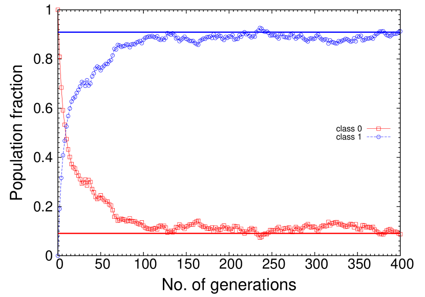
In simulations, we consider the population to be in steady state initially. This assumption is verified by ensuring that the population eventually reaches mutation-selection balance by observing single run plots corresponding to the given parameter set of , , and . Moreover, we confirm that the population fractions stabilize at values predicted by (A.5). Fig. G.1 in the Appendix shows qualitative comparison of the fixation probability of a non-mutator created at time in a population that is in steady state (filled symbols) with that of a non-mutator produced after a time interval of generations in a population which initially has no deleterious mutations (open symbols). In this article, each simulation point (excluding the points in the single run plot Fig. G.2) is averaged over independent stochastic runs. All simulations except those for Fig. G.1 have assumed . Apart from Fig. F.1, only non-mutators with have been considered here. All the numerical calculations have been done using Wolfram Mathematica .
2.2 Analysis
Due to the lower rates of deleterious mutation accumulation and fitness decline, the non-mutator appearing in mutator background in an adapted population is effectively a beneficial allele. The fixation probability of such an allele can be studied using the branching process (Patwa and Wahl, 2008). The details (Johnson and Barton, 2002) are described below.
The extinction probability of a non-mutator arising with deleterious mutations in generation in a very large population of mutators is given by
| (3) |
The above equation assumes that the extinction probabilities are independent of each other. Here, is the probability that the non-mutator will give rise to offspring in generation . is the Poisson distributed probability of the non-mutator to mutate from class to .
If the probability of reproduction of the non-mutator is assumed to be Poisson distributed, we get
| (4) |
In this expression, the mean of the Poisson distribution equals the absolute fitness of the non-mutator, and hence we write
| (5) |
Note that is the mean fitness of the background population with being the fraction of population having deleterious mutations in generation (see Appendix A for details on the expression for population fraction in steady state). With the help of (4) and (5), we rewrite (3) as
| (6) |
The non-mutators are considered established if they do not go extinct. Due to the selective advantage possessed by the non-mutator, the establishment eventually leads to fixation, and these two are taken to be the same here. Hence, the fixation probability is . Therefore, from (6), it follows that
| (7) |
since . For a non-mutator that arises in the background population after the attainment of steady state, (7) becomes
| (8) |
We get the fixation probability of a non-mutator that is produced in a genetic background having number of deleterious mutations by solving (8). However, the mutator population is distributed across so many fitness classes, and the non-mutator can appear in any of these backgrounds. Hence, the total fixation probability can be calculated only by taking into account all the possible genetic backgrounds. The probability of the non-mutator to appear in fitness class is the same as the fraction of the background population in that class. This is an important concept which plays a major role in understanding the results. As explained above, the total fixation probability receives contributions from both the fraction of background population and the probability of fixation, and therefore, can be expressed as
| (9) |
The above expression is applicable for very large populations in which the effect of genetic drift can be neglected.
3 Results
As considered by James and Jain (2016), for strong mutators which have very high mutation rates ( ) compared to the non-mutator (Sniegowski et al., 1997; Oliver et al., 2000), we can neglect to write
| (10) |
If the non-mutator has negligible mutation rate, we can directly obtain (10) from (3) assuming steady state, since . Using (A.4), the average fitness of mutators in steady state is found to be . This is otherwise the classical result obtained by Haldane (1937) for the mean fitness of an asexual population. Following the approach of James and Jain (2016), taking logarithm on both sides of (10), and neglecting terms of order greater than from the expansion , we can solve the resulting quadratic equation to get
| (11) |
Here, is the largest integer corresponding to , and is given by (A.4). We see that with rise in the background mutation rate , increases, which is rather expected. The intuitive meaning of (11) is that the effective selective advantage of a non-mutator carrying mutations, appearing in the background having mean fitness is , and its fixation probability is twice that. The latter statement follows from the single locus model (Fisher, 1922; Haldane, 1927).
Plugging (A.5) and (11) in (9), and performing the resulting sum give rise to
| (12) |
The derivations for the frequency of the background population with zero deleterious mutation are given in Appendices A and B, and the final expressions are summarized in Table 1. Based on whether the selection is strong () or weak () and the epistasis is antagonistic () or synergistic (), there are four regimes for .
| Class mutator frequency | ||
|---|---|---|
3.1 Variation of fixation probability with epistasis parameter
3.1.1 Weak selection; antagonistic epistasis ( , )
For large , with the help of Stirling’s approximation , we obtain
| (13) |
Using the result from Table 1, we get
| (14) |
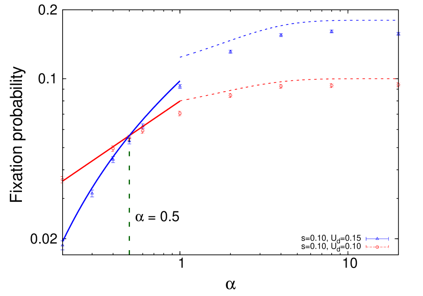
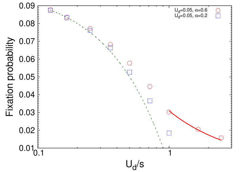
Expression (14) yields the known result (James and Jain, 2016) for . It is evident that , implying the total fixation probability to be an increasing function of the background mutation rate for and decreasing function for , as shown in Fig. 1. The value of at which this transition happens is denoted as , the critical value of the epistasis parameter. Corresponding to , (14) gives . As the mutation rate of a population increases, we expect it to have higher probability to reduce its mutation rate. However, if , we see that the higher the mutation rate of a population, the lower is the probability that its mutation rate will decrease. The physical interpretation of this surprising trend is explained in the following paragraph.
Combining (B.2) and (B.5) enables us to write
| (15) |
This clearly states that the background population frequency , which is also equal to the probability of the non-mutator to appear with deleterious mutations, is a Gaussian distribution with mean and variance . Therefore, in the regime and , the mutator population will be more spread out for larger values of and smaller values of .
As increases, it is more likely that the non-mutator will appear with higher number of deleterious mutations, which is disadvantageous to the invader population. However, as we saw in (11), once the non-mutator appears with a particular number of mutations, its fixation probability increases with . This is an advantageous factor associated with . Competition between the advantageous and disadvantageous effects of on the non-mutator decides the behavior of its total fixation probability as a function of . As falls below , the disadvantage experienced by the lower mutation rate allele due to its low fitness dominates its advantage of arising in a background that has high mutation rate.
Fig. 1, 3, and 5 show that the trend predicted by (14) is observed in finite size populations. Further, in the parameter regime used in the plot, (14) is a good approximation for the total fixation probability of a lower mutation rate individual in the strong mutator background.
It has to be noted that the result is valid only for the strong mutator background. A discussion on for the case in which the mutation rates of the non-mutator and mutator are comparable (weak mutator background) can be found in Appendix F.
3.1.2 Weak selection; synergistic epistasis ( , )
We have an analytical expression for only for the limiting case ( ), which is given in Table 1. The mutation rates of asexual microbes such as E. coli and S. cerevisiae are measured to be of the order of per genome per generation (Drake et al., 1998). The value of selection coefficient for E. coli is found to vary from (Gallet et al., 2012) to (, Lenski et al.1991). Even for the maximum value of in this case, which is 100, ensures that only the first two classes contribute to . In fact, even if , which could be biologically improbable, guarantees that for . This physically corresponds to two or more mutations interacting with each other to produce lethal effects on the genome. This is illustrated in Fig. G.2 in the Appendix. Therefore, it follows from (12) that
| (16) |
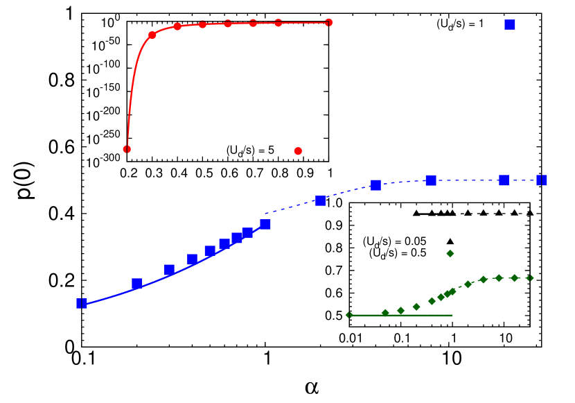
Here, the dependence of comes from . For , epistasis affects neither the fixation probability nor the fraction of background population of the first two fitness classes. Unsurprisingly, it can be seen that rises with increase in initially and reaches its maximum value , which is independent of . This is captured in Fig. 1 (also, see Appendix D where the discrepancy between the results from simulations and analytics has been discussed). It is important to note that if the condition is not satisfied, the non-mutator can arise in fitness classes having low fitness. Owing to this, (16) overestimates the actual value of .
Note that for and , (16) simplifies to the known result for fixation probability (James and Jain, 2016) of a non-mutator on a non-epistatic fitness landscape, when the selective effects are strong with respect to mutation rate. From (A.5) and (B.6), we see that synergistic epistasis with causes the background population to be concentrated around fitness class , and therefore, for . The fixation probability of a non-mutator with a single deleterious mutation is from (11) when . Thus, both and give the same results as and , respectively when selection is very strong and epistasis is either absent (James and Jain, 2016) or synergistic (see section 3.1.4). Effectively, the fitness class for and “replaces” fitness class for and . Fig. 4 shows variation of (16) with .
3.1.3 Strong selection; antagonistic epistasis ( , )
As , , and hence the fixation probability receives contribution only from class . Using the result from Table 1 in (12), we obtain
| (17) |
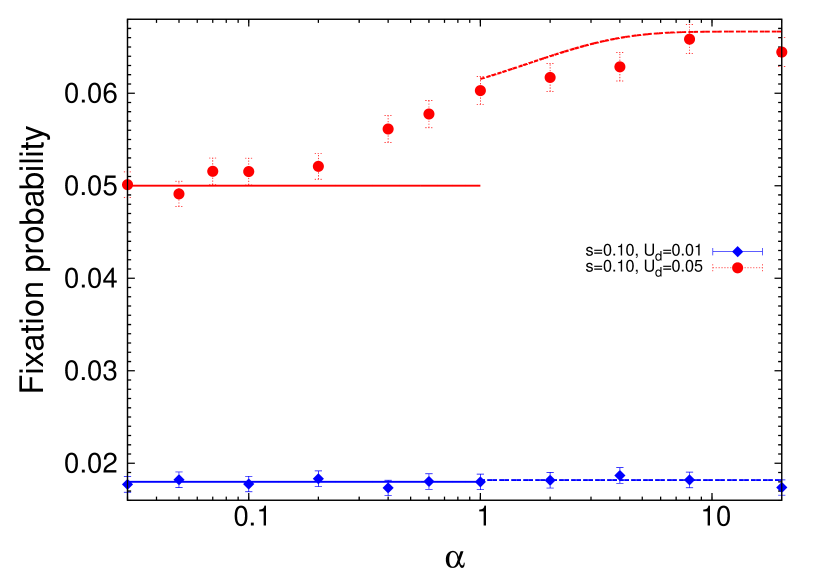
Fig. 2, 3 and 5 show the validity of (17) by comparing against finite population simulations. For values comparable to , if the condition is not fulfilled, the expression for is not valid (see Table B.1, and Case III in Appendix B). From Fig. 3 and 5, we can infer that for , varies with . For , is independent of .
3.1.4 Strong selection; synergistic epistasis ( , )
Since , the use of the result from Table 1 in (12) yields
| (18) |
As in the case of (16), with increase in , the dependence of on epistasis will vanish, and (18) will approach the constant value . Fig. 2 and 4 show the comparison of (18) with finite population simulations (a discussion on the discrepancy between the results from simulations and analytics can be found in Appendix D). Table 2 gives summary of all the results from section 3.
It is obvious that, for , (17) and (18) approach the known result for fixation probability (James and Jain, 2016) in the absence of epistasis ( ). This can also be obtained using a single locus model, since the population consists only of class individuals, and the selective advantage of non-mutators is the difference in the class frequencies. As the class individuals remain unaffected by epistasis for very strong selection, , which receives contribution only from class , is independent of .
3.2 Variation of fixation probability with mutation rate
3.2.1 Strong selection; antagonistic epistasis ( , )
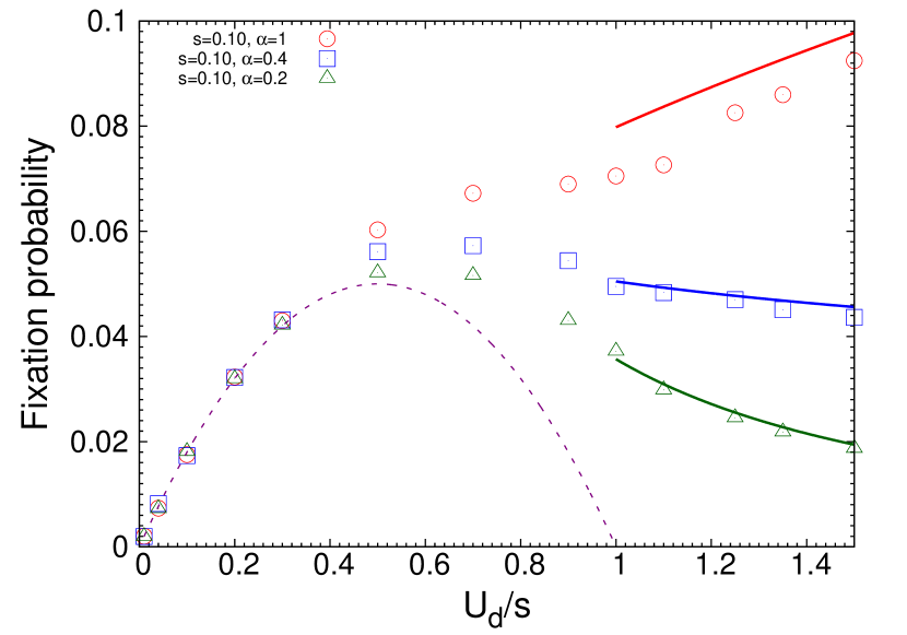
When we vary keeping to be the same, for , only the class individuals decide . For , (see Table 1). This means that a mutation is very costly, due to which any individual carrying it will not survive. As the number of mutators in class decreases with the rise in , a reduction in the mutation rate will be highly favored. Thus, increases with . For , depends on epistasis (Fig. 3 and 5), though the dependence is not analytically captured. This is because depends on . An increase (decrease) in () leads to decrease in (see Table B.1 and Fig. B.1), as the background population spreads out more. On the other hand, . This results in showing dependent behavior for similar to that in the regime , .
3.2.2 Weak selection; antagonistic epistasis ( , )
As discussed in section 3.1.1, the total fixation probability in the regime is a multilocus problem. For antagonistic epistasis, the non-mutator has higher chances of appearing in a lower fit background for larger values of . When , this disadvantage cannot be compensated by its benefit associated with being created in a higher mutation rate background. Due to this, falls as a function of . These two factors together give rise to a non-monotonic behavior of with respect to for , as shown in Fig. 3. If , we see that the advantage conferred by the non-mutator owing to being produced in a high mutation rate background dominates its drawback and therefore, increases with . Thus, is a monotonically increasing function of for (see Fig. 3).
3.2.3 Synergistic epistasis ( )
3.2.4 Effect of very large or small when is held constant
As increases to very large values relative to selection, for () , approaches (). Note that can never exceed . When is decreased to very small values compared to , falls towards irrespective of . This is obvious because the lower the mutation rate of the mutator is, the smaller the advantage associated with the reduction of mutation rate.
3.3 Variation of fixation probability with selection
3.3.1 Antagonistic epistasis ( )
The selection coefficient decides the effect of a mutation. Since the expression (17) for and is inadequate to capture the dependence, the simulation data corresponding to two values have been plotted for that regime in Fig. 5. Qualitatively, one can conclude that increases with . When is large, the non-mutator has a higher advantage by virtue of the higher deleterious effect of a mutation. For , it is possible to understand from (17) that becomes independent of , since it is determined only by the individuals that do not undergo mutation. In the weak selection regime, better understanding is possible with the help of (14), which is plotted in Fig. 5 for . When , for the given set of parameters and population size (), a steady state does not exist in the weak selection regime. Hence, the corresponding data is not shown in Fig. 5.
3.3.2 Synergistic epistasis ( )
For synergistic epistasis, in the special case of , an exact solution exists for . With the help of the result in Table 1, (12) becomes
| (19) |
which is valid for any value of . Corresponding to , , by which (19) takes the form
| (20) |
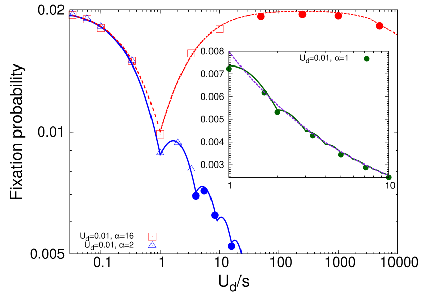
Fig. 4 shows the comparison of (19) with simulation data, which is represented using the blue open triangles. For the values of corresponding to which a population of size do not have steady state, the numerical solutions of (8) and (9) using Wolfram Mathematica are shown using the filled circles in the main figure in Fig. 4. Since we assumed and used the approximation (11), (19) overestimates the exact numerical solution by a small amount. The comparison of (19) with the exact solution using (8) and (9) is given in the last two columns of Table C.1. The detailed explanation for the surprising trend in Fig. 4 is given in Appendix C.
3.3.3 Effect of very large or small when is kept the same
We know from sections 3.1.3 and 3.1.4 that when , assumes the value regardless of . Expressions (20) and (C.4) also justify this claim, as the denominators of them approach for . When selection is reduced to much lower values compared to mutation rate, . This can be seen from (14) for , and Fig. 4 for . This is because there will not be any significant difference between mutators and non-mutators when the selective effects are negligibly small.
| Analytical expressions for | ||
|---|---|---|
| (Fig. 1) | (Fig. 2) | |
| (Fig. 3 5) | ||
| (Fig. 4) | ||
| (Fig. 4) | ||
4 Discussion
4.1 Summary of results and connection with real populations
In an asexual adapted population, it is known that (Jain, 2008) in the presence of synergistic epistasis, a higher proportion of individuals will carry less mutations, while in the presence of antagonistic epistasis, the fraction of individuals containing less mutations will be very low. In this article, it is found that antagonistic epistasis lowers the fixation probability of a lower mutation rate allele, thereby opposing the decline in mutation rate, while synergistic epistasis favors the reduction in mutation rate. Using a model similar to the one in this article, Kondrashov (1994) hypothesized that asexual populations could resist mutation accumulation in the presence of synergistic interactions. However, the model here assumes the population size to be a constant in every generation, while the size of an actual population fluctuates stochastically. A theoretical study in which the population size was allowed to vary with time (Gabriel et al., 1993) revealed that the extinction time of asexuals by virtue of onslaught of detrimental mutations vary depending on the values of parameters such as mutation rate, selection, etc. Since epistasis influences mutation rate reduction, results in the present article can be connected to the analysis of Gabriel et al. (1993) to unravel the role of epistasis on the extinction time of asexuals. However, real populations can have compensatory or back mutations (see two different models that incorporate compensatory mutations - John and Jain (2015); James and Jain (2016)) acting against the influx of deleterious mutations, which were neglected by all the above studies. In order to understand the fate of real asexual populations, the current study has to be extended by including more realistic considerations as discussed above.
It is observed in this study that there exists a critical value of epistasis below which the probability of reduction of mutation rate in an infinite population shows negative correlation with its mutation rate. For strong mutators, is found to be at using analytical arguments (see Appendices D and F). Though the mutation rate reduction happens with a non-zero probability, which is characteristic of any beneficial mutation, the decline in mutation rate becomes more unlikely when . For , the fixation probability of a non-mutator decreases with in the weak selection regime, as the lower mutation rate allele now appears with large number of mutations and finds it difficult to outcompete the resident population. On the other hand, increases with in the strong selection regime because of the non-mutator arising in class benefiting from the reduction of mutational load by a larger amount. (A discussion on in the weak mutator background is given in Appendix F.)
In the presence of synergistic interactions, initially remains constant at the value followed by a reduction, as is reduced in the strong selection regime. In the weak selection regime, as drops, manifests a non-monotonic behavior for every , where , but experiences eventual decay. This is shown in Fig. 4.
4.2 Limitations of the models and future goals
One major assumption which we have made in this article is that the population attains steady state after a large number of generations. However, populations of small size (see section 2.1 and Appendix E) do not have steady state, and hence the results presented here are not applicable to them. It is possible to evaluate the total fixation probabilities of non-mutators in such populations using (7) and (A.1). The total fixation probability will depend on the time of arrival of the non-mutator. This has been studied by Lynch (2011) for a non-epistatic landscape, when the selective effects are very strong. It is an open question for the epistatic landscape, and is not done here. The analysis in this article is a special case of this problem.
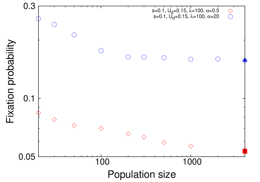
However, Fig. G.1 in the Appendix helps to have a qualitative understanding of the effect of variation of . For each value of in the figure, the non-mutator appears after generations. It is noticeable that large populations are more effective in withstanding the accumulation of harmful mutations. Small populations that are incapable of resisting the build-up of deleterious mutations and decline of mean fitness will be benefited more from the reduction in mutation rate. As a result, when increases, the fixation probability decreases and approaches the constant value predicted by (9). Articles like Lynch (2010, 2011); Jain and Nagar (2012); Sung et al. (2012); James and Jain (2016), etc. give insights into the role of population size on mutation rate evolution.
It is noteworthy that the model in this article examines the fixation probability of a single non-mutator appearing in the mutator population as described using (3). Its fixation is decided by whether the lineage of this particular non-mutator takes over the population or not. In reality, there can be multiple non-mutators emerging in the population. The article by Johnson and Barton (2002) includes the study of fixation probability of beneficial alleles arising at a constant rate. The same approach can be used to model the fate of multiple non-mutators arising in the adapted mutator population, since the non-mutator is effectively beneficial.
Actual biological populations may not have all the mutations having the same selective effects. There are models in which the selection coefficient is chosen from a distribution. However, the robustness of the results presented here could be tested using other fitness functions. There have been works taking into account the possible physiological costs associated with lowering the mutation rates (Kimura, 1967; Kondrashov, 1995; Dawson, 1998; Johnson, 1999; Baer et al., 2007). The effect of this factor could be explored.
4.3 Choice of parameters and biological relevance
Maisnier-Patin et al. (2005) experimentally confirmed that in Salmonella typhimurium, for various values of the mutation rates, the fitness effect of the mutations resembles the function (1) with . Synergistic epistasis has been observed in experiments (Mukai, 1969; Whitlock and Bourguet, 2000). In Drosophila melanogaster, the logarithm of relative productivity of genotypes was measured to be proportional to negative of the number of mutant regions carried by them (Whitlock and Bourguet, 2000). This is similar to the fitness function (1) with the corresponding being . In previous theoretical studies, the chosen values for range from (Fumagalli et al., 2015) to (Campos, 2004), whereas has been varied from to in the simulations in this article. The strength of the mutator can be as large as (Miller, 1996) to as small as around (McDonald et al., 2012; Wielgoss et al., 2013). In this study, values ranging from to (see Appendix F) are used. For E. coli populations, is observed to be in the range (Gallet et al., 2012) (, Lenski et al.1991), while per genome per generation (Drake et al., 1998). The present article includes values of and the absolute values of mutation rate (for both mutators and non-mutators) in the range and per genome per generation, respectively. In the experiment by Maisnier-Patin et al. (2005), was varied from to per genome per replication, and was measured to be .
With the help of information about the parameters , and from the experiment of Maisnier-Patin et al. (2005), it follows from (A.6) that lies between and corresponding to the lower and upper limits of . By including the selection coefficient, the condition proposed by Kondrashov (1994) can be modified to write , where is the minimum value of so as to have a steady state (see Appendix E). Hence, for the experiment of Maisnier-Patin et al. (2005), varies from to . Nevertheless, the population size in this case was . For this value of , a steady state is possible for . Therefore, to the best of our knowledge, Salmonella typhimurium is the only model organism which can be used to test the results in this article, as it is the only asexual for which has been measured.
4.4 Fixation time and comparison with experiments
The time required for the fixation of a non-mutator is given by the inverse of the rate at which non-mutators that are certain to get fixed are created (Weinreich and Chao, 2005). (The details of the fixation time can be found in Ewens (2004).) The rate of creation of non-mutators that are expected to reach fixation is the product of their rate of production and fixation probability. Thus, for a large population, the fixation time (James and Jain, 2016) is , where is the rate at which the mutation that produces the lower mutation rate allele happens, provided .
Table of Wielgoss et al. (2013) gives the mutation rate corresponding to genotypes and their respective times of origin. Assuming the time of origin corresponds to the time when a genotype was significantly high in proportion in order to get detected, we see that the time for reduction of mutation rate is inversely proportional to magnitude of the reduction. However, the experiment of McDonald et al. (2012) indicates that this reduction time is higher for a higher magnitude of decline in the mutation rate. The opposite trends observed in the above two experiments can be explained if epistasis is assumed to be present, as the fixation probability can be either an increasing or decreasing function of mutation rate depending on the epistasis parameter.
4.5 Comparison with previous theoretical works
It is known that the fixation probability of an allele with effective selective advantage in a finite population of size is (Kimura, 1962). In this model, for infinite population size, , as discussed in James and Jain (2016). That is, the fixation probability of a beneficial allele in an infinite population is twice its net selective advantage. For a harmful allele, is negative, and hence, its fixation probability (time) falls (increases) exponentially with (Kimura, 1980; Assaf and Mobilia, 2011).
Fixation of mutators in an asexual non-mutator population is effectively the same as fixation of a harmful allele if the fitness affecting beneficial mutations are excluded. For this problem, Jain and Nagar (2012) studied the fixation time of mutators, and the time was found to increase exponentially ( for weak selection, and for strong selection). It is important to be noted that we study only the strong mutator case ( ). From the above mentioned result of Jain and Nagar (2012), we can obtain the effective selective disadvantage conferred by the mutator (which is also the same as ) to be for weak selection. This has similar dependence on as (14), though the mutator strength does not enter our expression. For , these two solutions differ only by a factor . Nevertheless, in the strong selection regime, the net selective disadvantage of the mutator is simply , which exactly matches with our result. In the case of the work of Jain and Nagar (2012), there is a continuous production of mutators from non-mutators owing to which mutators sweep to fixation in a finite population. For a population of large size, the corresponding steady state fitness is In the present article, we analyze a mutator population that is in steady state initially with mean fitness . The non-mutator allele can appear in a background carrying mutations, and reach fixation to form a distribution of non-mutators with mean fitness . Though the initial state of the problem addressed in this article is the same as the final state of the problem considered by Jain and Nagar (2012), the reverse is not true. In the special case of strong selection, these two articles study “complementary” processes.
Acknowledgements
The author is thankful to CSIR for the funding as well as K. Jain, K. Zeng, and B. Charlesworth for the discussions. The author is grateful to K. Jain for some valuable comments and two anonymous reviewers for their suggestions. The author extends his thanks to Vinutha L. for her help with proofreading and editing the manuscript.
Appendix A Frequency of mutator population
When and are small, the population fraction of mutators carrying mutations in generation can be expressed using the equation
| (A.1) |
where
| (A.2) |
When the population is in steady state, (A.1) and (A.2) become time independent, and we get
| (A.3) |
Solving (A.3) for yields expression for negative of the mean Wrightian fitness (logarithm of the Malthusian fitness given by (1)) of the population per selection coefficient
| (A.4) |
This can be substituted back in (A.3) and iterated to get (Jain, 2008)
| (A.5) |
The normalization condition gives (Jain, 2008)
| (A.6) |
The exact solutions to the above expression are possible only for (non-epistatic case) (Kimura and Maruyama, 1966; Haigh, 1978) and (Jain, 2008).
| (A.7) |
is the modified Bessel function of the first kind of order . (Refer to Abramowitz and Stegun (1964) to know more about this function.) It is a monotonically increasing function of , so that decreases with increase in . For any value of except and , approximations are needed to solve (A.6).
Appendix B Approximate expressions for the class zero mutator frequency
By taking the ratio in (A.5), we can see that the maximum of is at .
Case I: ,
For , when selection is weaker than mutation rate, . Correspondingly, the distribution of mutators can be approximated by a Gaussian. As a first step, upon using Stirling’s approximation in (A.5), we obtain
| (B.1) |
Now, converting (B.1) to an exponential and then expanding around its maximum using Taylor series gives
| (B.2) |
By replacing the sum in (A.6) by an integral and using (B.2), we get
| (B.3) |
Performing the integral in (B.3) yields
| (B.4) |
For large values of , we have the expansion . By using this, we can simplify (B.4) to write
| (B.5) |
Note that (B.5) reproduces the known result for . Fig. B.1 shows a comparison of (B.5) with (A.6). The inset at the left top clearly indicates that (B.5) very well captures the exact sum even for extremely small values of .
Case II: ,
In this case, the Gaussian approximation does not hold good. An approximate solution is possible for the limit case . When , the mutator frequency peaks around (also, see section 3.1.2), and contributions to from classes with are negligibly small. Nevertheless, in order to obtain a very accurate estimate of , terms up to second order can be retained. Effectively, we get
| (B.6) |
As increases, rises to the constant value , which is the upper bound of . Fig. B.1 shows that (B.6) matches well with (A.6) for large values of . For values of that are not very large, other classes also contribute. As a result, will be smaller than what is predicted by (B.6).
Case III: ,
When , in (A.5) is a monotonically decreasing function of . In the limiting case , (A.6) becomes
| (B.7) |
However, (B.7) only provides the lower bound of in the presence of antagonistic epistasis when the selection is strong. When both and are not very small compared to , this expression is not accurate to obtain the exact values of (see Table B.1). The right bottom inset of Fig. B.1 shows that predicted by (A.6) decreases to (B.7) for very small values of . It can be seen that depends on if the numerical value of is close to . Expression (B.7) does not capture this dependence. When , becomes independent of . Moreover, Table B.1 and Fig. B.1 indicate that corresponding to the same value of , as the value of increases, decreases.
Note that when , it follows from (1) that all the individuals carrying non-zero mutations have the same fitness . Thus, in practice, the population has only two classes differing in fitness by , with mutation rate from class to being . For this, the steady state solution for population fraction in class yields (B.7).
| Comparison of (B.7) with (A.6) | |||
|---|---|---|---|
| (exact) | |||
Case IV: ,
Like Case II studied here, the class mutator fraction increases with .
| (B.8) |
From the right bottom inset of Fig. B.1, we can see that predicted by (A.6) increases to for large values of . When , (B.7) and (B.8) give almost the same result close to for , indicating the fact that the fraction of individuals with zero deleterious mutations in the population is unaffected by epistasis when the selective effects are very strong. Since the population is localized around class , the frequency of individuals in other fitness classes will be insignificant. Note that when is not very small compared to , depends on .
Results of this section are summarized in Table 1.
Appendix C Explanation for the trend in Fig. 4
Table C.1 gives the numerical values of using (8), and for different values of . When is reduced, remains roughly the same, while decreases. This explains why falls as a function of in the strong selection regime. For , for a given value of , (see (11)) increases with decrease in . From Appendix B, we understand that the distribution peaks around . Column of Table C.1 shows this value. The integer part of the corresponding number gives the maximum value of the fitness class that contributes to . In the weak selection regime, when is lowered keeping to be the same, we see from Table C.1 that remains almost the same, while decreases for all . Hence, the net effect on due to decrease in is not a straightforward problem. To have a better understanding at least for ( ), we can make use of (16). The argument used in understanding the case can be extrapolated to the general case , where takes only positive integer values.
By taking the first derivative of in (16) with regard to , we can see that peaks at a particular value of selection
| (C.1) |
Note that for , (C.1) yields ( ), which approximately matches with the simulation data (blue triangles) shown in Fig. 4, whereas for (shown using the red squares), ( ). The latter point also agrees with the data plotted in Fig. 4. The red curves for the weak and strong selection regimes are (16) and (18), respectively. increases with decrease in for . Further decrement in reduces for . When is lowered from to , where (see Table C.1), increases by . Consequently, frequencies of classes having high values decrease. For , declines rapidly with . This can be explicitly seen in the last row in Table C.1, for which the selection is very small. Therefore, each time increases by due to decrement in , increases initially, followed by a faster decay. As a result, whenever with being any non-zero value of , assumes its local minimum values, as we see in Fig. 4.
In the weak selection regime, for , undergoes damped oscillations and decreases overall. We will examine the properties of its local maxima or peaks. The relative increase in corresponding to (first peak) can be measured as
| (C.2) |
Substituting (C.1) in (16), we get
| (C.3) |
For , (C.3) yields , and (16) leads to . Indeed, these two match with the observed values in Fig. 4. Thus, we estimate the value of the relative increase in corresponding to to be percent for using (C.2). This result is applicable for any large value of for which . For , (C.1) can be substituted back in the exact expression (19) to obtain . At , using (19), . These two results also are in good agreement with what is observed in Fig. 4. The resulting relative increase in for corresponding to is percent. It is evident that with reduction in , the first peak gets smaller. Moreover, Fig. 4 suggests that for the same value of , the peaks associated with further reductions in ( ) become less significant.
For , the approximation was made in order to get the simple analytical expression (14). At least for , for which an exact formula for is available, the presence of non-monotonicity in the weak selection regime can be tested. Using (A.7) in (12), we can write
| (C.4) |
In the weak selection regime, when , this can be rewritten as . By differentiating with respect to , one can see that peaks at . However, in this section, we have already seen that the local minima of occur at . This reflects the fact that there is no non-monotonicity for . The inset of Fig. 4 shows (C.4) using dark green lines, and the filled circles are the numerical solutions of using (8) and (9). The broken violet line is the approximate expression (14) for . For antagonistic epistasis, from the simulation data in Figures 3 and 5, we do not see any non-monotonic trend in the weak selection regime unlike Fig. 4. Note that for the set of parameters used in these two figures, can be as large as .
| Synergistic epistasis: Variation of with selection | |||||||||||
| Exact | Eqn. (19) | ||||||||||
Appendix D Regarding the discrepancy between the analytical and simulation results
To have a steady state, the size of a population needs to be of the order of (Kondrashov, 1994). Table D.1 gives values by solving (B.5) corresponding to two values, changing . For large and small , we find that the size required for the attainment of steady state is too large for most of the biological populations. Hence, populations of lower size will accumulate deleterious mutations and go extinct (see section 4.1). By comparing columns and , it can be seen that as decreases, (14) deviates from the exact solution of obtained using (8) and (9). This is because the approximation (11) does not hold good for the fitness classes close to , which contribute more to due to the form (15) taken by the mutator frequency. Moreover, for a particular value of , the deviation is less if the value of is small. Nevertheless, populations of size in the biological limit having larger values of and smaller values of do not have steady state. Hence, (14) is applicable to most of the real populations except those with both and antagonistic epistasis with very small values. However, a better approximation to is needed to yield more accurate results for when and .
One more thing to note is that is obtained using (14). This tells us that the “true” value of could be slightly different from , as (14) deviates from the exact results. The best estimate of is given in Appendix F.
| Weak selection; antagonistic epistasis: | ||||
| Comparison of (14) with the exact numerical solution for | ||||
| Exact value of | using (14) | |||
| using (8) and (9) | ||||
To derive (11), we assumed that and neglected cubic and higher order terms. When , values will differ from what we obtain using (11). Due to the same reason, there is discrepancy between (16) and (18), as well as the simulation data in Figures 1 and 2, respectively. The same expressions match well with the simulation points for as shown in Fig. 4 and using the blue diamonds in Fig. 2. Corresponding to the point , Table D.2 provides a comparison of (16) and (18), and the simulation results in Figures 1 and 2, respectively. In fact, (14) also deviates from the simulation results for large values. This is clear in the case of the red circles corresponding to and the blue squares corresponding to in Fig. 3, and in Fig. 1, where scale is used to plot the data. Moreover, based on the discussion in Appendix C, it is worth noting that (12) is the more accurate form of (14), but the latter is more simplified.
| Synergistic epistasis: Comparison of simulation data in | |||
|---|---|---|---|
| Figures 1 and 2 with analytical results | |||
| (standard error) | |||
The analytical expression (17) for the strong selection; antagonistic epistasis regime (section 3.1.3) is valid only for . A more precise formula for in this case can help us to analytically understand the variation of with , and the non-monotonic behavior in Fig. 3. Further, (16) and (18) are not exact expressions. A more accurate expression for in the presence of synergistic epistasis will pave the way for better analytical understanding.
Appendix E Regarding steady state
The argument of Kondrashov (1994) on the minimum population size necessary to ensure steady state includes only the population fraction corresponding to the least loaded class (see section 2.1). A further detailed analysis by Jain (2008) shows that the ratchet time is actually proportional to the number of individuals in the least loaded class times the selection coefficient. A very high ratchet time corresponds to very a slowly operating ratchet. For smaller values of selection coefficient, the deviation from the results of Kondrashov (1994) becomes clearer. Nevertheless, for the parameters used in this article, there will not be any significant difference from the above theory, since smaller values of selection have been used only for synergistic epistasis.
Appendix F Critical value of epistasis for the weak mutator background
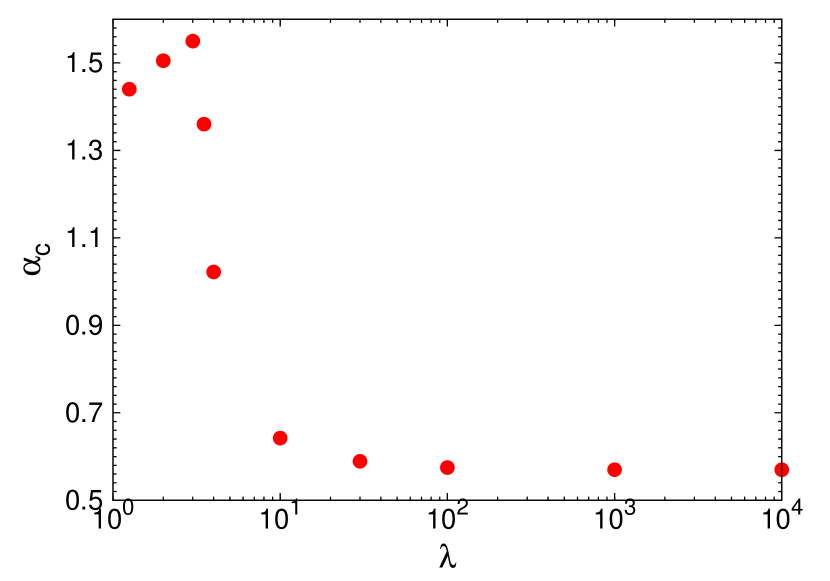
Weak mutator refers to the case when the mutation rate of the non-mutator is comparable ( ) with that of the mutator. In two recent mutation reduction experiments (McDonald et al., 2012; Wielgoss et al., 2013), weak mutators with as low as have been observed. By solving (8) and (9) using Wolfram Mathematica , we obtain as a function of for a given value of . By comparing these values up to three significant figures for two different values of , we estimate corresponding to each . With the variation in mutator strength, changes. This is plotted in Fig. F.1. For strong mutators, the exact numerical analysis suggests that approaches its minimum value , as . This is contrary to the analytical result using (14). Therefore, even though (14) is helpful in demonstrating the presence of (see section 3.1.1), this expression is not very accurate in determining precisely. This is because of the two approximations (B.5) and (11) involved in the derivation of (14) (see Appendix D as well). As falls towards , rises to its upper limit . A further reduction in results in decrease in .
The interpretation for the initial increase of with decrease in is as follows: A significantly high deleterious mutation rate reduces the fixation probability of non-mutator, since it is a disadvantageous factor. Thus, a non-mutator produced in a weak mutator background that is less spread out, and that created in a strong mutator background which is more spread out can have the same fixation probabilities. The former and latter respectively correspond to larger and smaller values of . Therefore, the critical value of the epistasis parameter rises as the strength of the mutator decreases. However, the decline of with for is counterintuitive. The explanation for this interesting trend requires a detailed analysis. A study of the weak mutator case is beyond the scope of this article and will be left for a separate work. The results presented regarding weak mutators is meant to give directions for future work. Solving (8) without neglecting will be useful in obtaining analytical expressions in this case.
Table F.1 gives the data from finite simulations for three values of . Using this, a crude estimate of has been made corresponding to each . The errors associated with are not given, since the error calculation is not straightforward here. Nevertheless, we see a clear variation with respect to , similar to what we see from the exact numerical solution.
| Simulation results for weak mutators | |||||||
|---|---|---|---|---|---|---|---|
| 1.6 | 1.6 | ||||||
| 0.9 | 0.9 | ||||||
| 0.5 | 0.5 | ||||||
Appendix G Supplementary figures
References
- Assaf and Mobilia (2011) Assaf, M. and M. Mobilia, 2011 Fixation of a deleterious allele under mutation pressure and finite selection intensity. J. Theo. Biol. 275: 93–103.
- Abramowitz and Stegun (1964) Abramowitz, M. and I. Stegun, 1964 Handbook of mathematical functions with formulas, graphs, and mathematical tables. Dover, New York.
- Baer et al. (2007) Baer, C. F. M. M. Miyamoto, and D. R. Denver, 2007 Mutation rate variation in multicellular eukaryotes. Nat. Rev. Genet. 8: 619–631.
- Campos (2004) Campos, P. R. A., 2004 Fixation of beneficial mutations in the presence of epistatic interactions. Bull. Math. Biol. 66: 473–486.
- Charlesworth and Charlesworth (2010) Charlesworth, B. and D. Charlesworth, 2010 Elements of evolutionary genetics. Roberts and company.
- Chou et al. (2011) Chou, H. , H. Chiu, N. F. Delaney, D. Segre, and C. J. Marx, 2011 Diminishing returns epistasis among beneficial mutations decelerates adaptation. Science 332: 1190–1192.
- Cumming et al. (2007) Cumming, G. F. Fidler, and D. L. Vaux, 2007 Error bars in experimental biology. J. Cell. Biol. 177: 7–11.
- Dawson (1998) Dawson, K., 1998 Evolutionarily stable mutation rates. J. Theor. Biol. 194: 143–157.
- Desai and Fisher (2011) Desai, M. M. and D. S. Fisher, 2011 The balance between mutators and nonmutators in asexual populations. Genetics 188: 997–1014.
- Drake et al. (1998) Drake, J. W., B. Charlesworth, D. Charlesworth, and J. F. Crow, 1998 Rates of spontaneous mutation. Genetics 148: 1667–1686.
- Ewens (2004) Ewens, W. J., 2004 Mathemtical population genetics I. Theoretical Introduction. Springer.
- Fisher (1922) Fisher, 1922 On the dominance ratio. Proc. Roy. Soc. Edinburgh. 52: 399–433.
- Fumagalli et al. (2015) Fumagalli, M. R., M. Osella, P. Thomen, F. Heslot, and M. C. Lagomarsino, 2015 Speed of evolution in large asexual populations with diminishing returns. J. Theor. Biol. 365: 23–31.
- Gabriel et al. (1993) Gabriel, W., M. Lynch, and R. Burger, 1993 Muller’s ratchet and mutational meltdowns. Evolution 47: 1744–1757.
- Gallet et al. (2012) Gallet, R., T. F. Cooper, S. F. Elena, and T. Lenormand, 2012 Measuring selection coefficients below : methods, questions and prospects. Genetics 190: 175–186.
- Giraud et al. (2001) Giraud, A., I. Matic, O. Tenaillon, A. Clara, M. Radman, M. Fons, and F. Taddei, 2001 Costs and benefits of high mutation rates: adaptive evolution of bacteria in the mouse gut. Science 291: 2606 – 2608.
- Haigh (1978) Haigh, 1978 The accumulation of deleterious genes in a population - Muller’s ratchet. Theor. Pop. Biol. 14: 251–267.
- Haldane (1927) Haldane, 1927 A mathematical theory of natural and artificial selection. V. Proc. Camb. Philos. Soc. 23: 838–844.
- Haldane (1937) Haldane, 1937 The effect of variation on fitness. Am. Nat. 71: 337–349.
- Jain and Krug (2007) Jain, K. and J. Krug, 2007 Adaptation in simple and complex fitness landscapes. In U. Bastolla, M. Porto, H. Roman, and M. Vendruscolo (Eds.), Structural approaches to sequence evolution: molecules, networks and populations, pp. 299–340. Springer, Berlin.
- Jain (2008) Jain, K., 2008 Loss of least loaded class in asexual populations due to drift and epistasis. Genetics 179: 2125–2134.
- Jain (2010) Jain, K., 2010 Time to fixation in the presence of recombination. Theor. Pop. Biol. 77: 23–31.
- Jain and Nagar (2012) Jain, K. and A. Nagar, 2012 Fixation of mutators in asexual populations: the role of genetic drift and epistasis. Evolution 67: 1143–1154.
- James and Jain (2016) James, A. and K. Jain, 2016 Fixation probability of rare nonmutator and evolution of mutation rates. Ecol. Evol. 6: 755–764. DOI: 10.1002/ece3.1932.
- John and Jain (2015) John, S. and K. Jain, 2015 Effect of drift, selection and recombination on the equilibrium frequency of deleterious mutations. J. Theor. Biol. 365: 238–246.
- Johnson (1999) Johnson, T., 1999 Beneficial mutations, hitchhiking and the evolution of mutation rates in sexual populations. Genetics 51: 1621–1631.
- Johnson and Barton (2002) Johnson, T. and N. Barton, 2002 The effect of deleterious alleles on adaptation in asexual populations. Genetics 162: 395–411.
- Khan et al. (2011) Khan, A. I., D. M. Dinh, D. Schneider, R. E. Lenski, and T. F. Cooper, 2011 Negative epistasis between beneficial mutations in an evolving bacterial population. Science 332: 1193–1196.
- Kimura (1962) Kimura, M., 1962 On the probability of fixation of mutant genes in a population. Genetics 47: 713–719.
- Kimura (1967) Kimura, M., 1967 On the evolutionary adjustment of spontaneous mutation rates. Genet. Res. 9: 23–34.
- Kimura (1980) Kimura, M., 1980 Average time until fixation of a mutant allele in a finite population under continued mutation pressure: studies by analytical, neumerical, and pseudo-sampling methods. Proc. Natl. Acad. Sci. USA 77: 522–526.
- Kimura and Maruyama (1966) Kimura, M. and T. Maruyama, 1966 The mutational load with epistatic gene interactions in fitness. Genetics 54: 1337–1351.
- Kondrashov (1994) Kondrashov, A., 1994 Muller’s ratchet under epistatic selection. Genetics 136: 1469–1473.
- Kondrashov (1995) Kondrashov, A., 1995 Modifiers of mutation-selection balance: general approach and the evolution of mutation rates. Genet. Res. 66: 53–69.
- (35) Kryazhimskiy, S., G. Tkacik, and J. B. Plotkin, 2009 The dynamics of adaptation on correlated fitness landscapes. Proc. Natl. Acad. Sci. USA 106: 18638–18643.
- (36) Lenski, R. E., M. R. Rose, S. C. Simpson, and S. C. Tadler, 1991 Long-term experimental evolution in Escherichia coli. I. Adaptation and divergence during 2,000 generations. Am. Nat. 138: 1315–1341.
- Liberman and Feldman (2013) Liberman, U. and M. Feldman, 1986 Modifiers of mutation rate: A general reduction principle. Theor. Pop. Biol. 30: 125–142.
- Lynch (2010) Lynch, M., 2010 Evolution of the mutation rate. Trends in Genetics 26: 345–352.
- Lynch (2011) Lynch, M., 2011 The lower bound to the evolution of mutation rates. Genome Evol. Biol. 3: 1107–1118.
- Maisnier-Patin et al. (2005) Maisnier-Patin, S., J.-R. Roth, A. Fredriksson, T. Nystrom, O. G. Berg, and D.-I. Andersson, 2005 Genomic buffering mitigates the effects of deleterious mutations in bacteria. Nat. Genet. 37: 1376–1379.
- McDonald et al. (2012) McDonald, M., Y.-Y. Hsieh, Y.-H. Yu, S.-L. Chang, and J.-Y. Leu, 2012 The evolution of low mutation rates in experimental mutator populations of Saccharomyces cerevisiae. Current Biology 22: 1235–1240.
- Miller (1996) Miller, J., 1996 Spontaneous mutators in bacteria: Insights into pathways of mutagenesis and repair. Annu. Rev. Microbiol. 50: 625–643.
- Mukai (1969) Mukai, T., 1969 The genetic structure of natural populations of Drosophila melanogaster. VII. Synergistic interaction of spontaneous mutant polygenes controlling viability. Genetics 61: 749–761.
- Notley-McRobb et al. (2002) Notley-McRobb, L., S. Seeto, and T. Ferenci, 2002 Enrichment and elimination of mutY mutators in Escherichia coli populations. Genetics 162: 1055–1062.
- Oliver et al. (2000) Oliver, A., R. Cantón, P. Campo, F. Baquero, and J. Blázquez, 2000 High frequency of hypermutable Pseudomonas aeruginosa in cystic fibrosis lung infection. Science 288: 1251–1253.
- Palmer and Lipsitch (2006) Palmer, M. and M. Lipsitch, 2006 The influence of hitchhiking and deleterious mutation upon asexual mutation rates. Genetics 173: 461–472.
- Patwa and Wahl (2008) Patwa, Z. and L. Wahl, 2008 The fixation probability of beneficial mutations. J. R. Soc. Interface 5: 1279–1289.
- Plucain et al. (2014) Plucain, J., T. Hindre, M. Le Gac, O. Tenaillon, S. Cruveiller, C. Medigue, N. Leiby, W. R. Harcombe, C. J. Marx, R. E. Lenski, and D. Schneider, 2014 Epistasis and allele specificity in the emergence of a stable polymorphism in Escherichia coli. Science 343: 1366–1369.
- Raynes and Sniegowski (2014) Raynes, Y. and P. Sniegowski, 2014 Experimental evolution and the dynamics of genomic mutation rate modifiers. Heredity 113: 375–380.
- Smith and Haigh (1974) Smith, J. M. and J. Haigh, 1974 Hitchhiking effect of a favourable gene. Genet. Res. 23: 23–35.
- Sniegowski et al. (1997) Sniegowski, P. D., P. J. Gerrish, and R. Lenski, 1997 Evolution of high mutation rates in experimental populations of E. coli. Nature 387: 703–705.
- Sniegowski and Gerrish (2010) Sniegowski, P. D., and P. J. Gerrish, 2010 Beneficial mutations and the dynamics of adaptation in asexual populations. Phil. Trans. R. Soc. B 365: 1255–1263.
- Söderberg and Berg (2011) Söderberg, R. and O. Berg, 2011 Kick-starting the ratchet: The fate of mutators in an asexual population. Genetics 187: 1129–1137.
- Sung et al. (2012) Sung, W., M. S. Ackerman, S. F. Miller, T. G. Doak, and M. Lynch, 2012 The drift-barrier hypothesis and mutation-rate evolution. Proc. Natl. Acad. Sci. USA 109: 18488–18492.
- Taddei et al. (1997) Taddei, T., M. Radman, J. Maynard-Smith, B. Toupance, P. H. Gouyon, and B. Godelle, 1997 Role of mutator alleles in adaptive evolution. Nature 387: 700–702.
- Tenaillon et al. (1999) Tenaillon, O., B. Toupance, H. Nagard, F. Taddei, and B. Godelle, 1999 Mutators, population size, adaptive landscape and the adaptation of asexual populations of bacteria. Genetics 152: 485–493.
- Tröbner and Piechocki (1984) Tröbner, W. and R. Piechocki, 1984 Selection against hypermutability in Escherichia coli during long-term evolution. Mol. Gen. Genet. 198: 177–178.
- Turrientes et al. (2013) Turrientes, M.-C., F. Baquero, B. Levin, J.-L. Martinez, A. Ripoll, J.-M. González-Alba, R. Tobes, M. Manrique, M.-R. Baquero, M.-J. Rodriguez-Dominguez, R. Cantón, and J.-C. Galńa, 2013 Normal mutation rate variants arise in a mutator (Mut S) Escherichia coli population. PLoS ONE 8: e72963.
- Weinreich and Chao (2005) Weinreich, D. M. and L. Chao, 2005 Rapid evolutionary escape by large populations from local fitness peaks is likely in nature. Evolution 59-6: 1175–1182.
- Whitlock and Bourguet (2000) Whitlock, M. C. and D. Bourguet, 2000 Factors affecting the genetic load in Drosophila: synergistic epistasis and correlations among fitness components. Evolution 54: 1654–1660.
- Wiehe (1997) Wiehe, T., 1997 Model dependency of error thresholds: the role of fitness functions and contrasts between the finite and infinite sites model. Genet. Res. Camb. 69: 127–136.
- Wielgoss et al. (2013) Wielgoss, S., J. Barrick, O. Tenaillon, M. Wiser, W. Dittmar, S. Cruveiller, B. Chane-Woon-Ming, C. Médigue, R. E. Lenski, and D. Schneider, 2013 Mutation rate dynamics in a bacterial population reflect tension between adaptation and genetic load. Proc. Natl. Acad. Sci. USA 110: 222–227.
- Wylie et al. (2009) Wylie, C., C.-M. Ghim, D. Kessler, and H. Levine, 2009 The fixation probability of rare mutators in finite asexual populations. Genetics 181: 1595–1612.