Over-the-barrier electron detachment in the hydrogen negative ion

Abstract

The electron detachment from the hydrogen negative ion in strong fields is studied using the two-electron and different single-electron models within the quasistatic approximation. A special attention is payed to over-the-barrier regime where the Stark saddle is suppressed below the lowest energy level. It is demonstrated that the single-electron description of the lowest state of ion, that is a good approximation for weak fields, fails in this and partially in the tunneling regime. The exact lowest state energies and detachment rates for the ion at different strengths of the applied field are determined by solving the eigenvalue problem of the full two-electron Hamiltonian. An accurate formula for the rate, that is valid in both regimes, is determined by fitting the exact data to the expression estimated using single-electron descriptions.

Although it is one of the simplest systems in atomic physics, the hydrogen negative ion (H^-) is still a subject of extensive experimental and theoretical studies. In early years of quantum mechanics at the focus of these studies was the ground state of the free ion. The existence of H^- as a bound system had been proposed theoretically by Bethe in 1929 bethe (see a historical review of H^- in Ref. rau and an overview in the context of negative ions in Ref. andersen ). Earlier predictions based on simple perturbational or variational methods (using, for example, the variational wave function $\psi\sim\exp[-a(r_{1}+r_{2})]$) had failed, even though these methods were well suited to predict the most of properties of other members of the two-electron isoelectronic sequence such as He, Li⁺, Be⁺⁺, etc. This is not surprising since the interaction between electrons in the hydrogen negative ion, unlike to helium atom and two-electron positive ions, is comparable in magnitude to that between the nucleus and electrons. As a consequence H^- is a weakly bound system which has only one bound state – the ground state. Its binding energy is $E_{\mathrm{B}}=0.7542$ eV (0.0277 a.u.) AHH ; LML ; radzig . A very weak binding and the absence of a long-range Coulomb attraction for the separated electron (the atomic residue is the neutral hydrogen atom) results in the fact that this two-electron system has no singly excited states.

The wave function and probability amplitude of a weakly bound system such as H^- can extend beyond the range of the binding potential itself. As it was recognized by Chandrasekhar more than 70 years ago chandra (see also Ref. rau ), the ground state wave function of H^- exhibits a specific radial correlation between the electrons such that one electron is bound much closer to the nucleus than the other which is weakly held at a distance of 4-5 Bohr radii from the nucleus. In contrast to the wave function with equivalent electrons $\psi\sim\exp[-a(r_{1}+r_{2})]$ (see Fig. 1(c)), the Chandrasekhar’s wave function of the form $\psi\sim\exp(-ar_{1}-br_{2})+\exp(-ar_{2}-br_{1})$ with the parameters $a=1.03925$, $b=0.28309$ (see Fig. 1(a)) provides the stability of H^- chandra . Regarding the electron detachment processes, such a configuration suggests a very useful one-electron picture where the outer electron is weakly (loosely) bound in a short-range attractive potential well. To a good approximation the potential acting on the outer electron due to the neutral atom is a sum of a short-range potential and the polarization term falling off as $1/r^{4}$ (see a short overview of the potentials of this type in the Appendix in Ref. gru-sim ). Moreover, since the outer electron spends much of the time beyond the potential well, it may be treated even as a free particle subject to boundary conditions imposed at the nucleus position. This simple model essentially takes the attraction to be of zero-range and it is in literature known as the zero-range potential (ZRP, see e.g. Ref. dem-ost ).

Beside strictly theoretical reasons, the earliest interest for studying H^- came from the atmosphere physics and astrophysics. The existence of the hydrogen negative ion in the Solar and other stars photospheres was first discussed in the literature by Wildt in 1939 wildt . In this study it was demonstrated that photo-absorption properties of H^- might be important for the opacity of these atmospheres. One of the possible processes which contribute to the atmospheric absorption coefficient is just the electron photo-detachment of this ion.

The single-photon detachment cross section for H^- has received a considerable amount of attention in the past (see Refs. rau ; andersen and references therein). At the threshold of this process (for one-electron ejection) the residual hydrogen atom is left in the ground state and no long-range forces act on the departing electron BH . The experimental cross section is found to be in a good agreement with the Wigner low that is a feature of short-range potentials LML . During the last two decades, intense lasers have made it possible to observe effects of multiphoton absorption by atoms and ions, including the hydrogen negative ion rau ; andersen . In contrast to the single-photon case, the multiphoton detachment may occur at the photon energies $\hbar\omega<E_{\mathrm{B}}$, but since the detachment rates in this case are significantly lower, in order to get a measurable effect one needs much stronger fields.

At larger intensities, however, another mechanism for the electron detachment arises – the quantum-mechanical tunneling. A strong field distorts the potential of atomic residue forming a potential barrier (Stark saddle) through which the electron can tunnel. Finally, at a sufficiently strong field the barrier is suppressed below the energy of the bound state. This regime can be referred to as over-the-barrier detachment (OBD). The transition from the multiphoton to the tunnelling regime is governed by the Keldysh parameter $\gamma=\omega\,(2m_{e}E_{\mathrm{B}})^{1/2}/eF$ keldysh , where $F$ is the peak value of the electric component of electromagnetic field. This parameter characterizes the degree of adiabaticity of the motion through or over the barrier: If $\gamma\gg 1$ (high-intensity–long-wavelength limit) multiphoton processes dominate, whereas for $\gamma\ll 1$ (low-intensity–short-wavelength limit) the tunneling or OBD mechanism does.

In the second case ($\gamma\ll 1$) the quasistatic description is a good approximation. It assumes that the electric field changes slowly enough that a static detachment rate can be calculated for each instantaneous value of the field. Then the detachment rate for the alternating field can be obtained by averaging the static rates over the field period. For this purpose it is sufficient to use the Hamiltonian (here and thereafter we use the atomic units)

$$H=-\frac{1}{2}(\Delta_{1}+\Delta_{2})-\frac{1}{r_{1}}-\frac{1}{r_{2}}+\frac{1}{r_{12}}-F(z_{1}+z_{2}),$$ (1)

describing the dynamics of two electrons of H^- in a static electric field $F$. Here $\mathbf{r}_{i}$ is the $i$-th electron’s position and $r_{12}=|\mathbf{r}_{1}-\mathbf{r}_{2}|$. Due to presence of the barrier all eigenstates of (1) have the resonant character when $F\neq 0$, including the lowest which is an exact bound state for $F=0$. The width $\Gamma$ of the lowest state determines the electron detachment rate $w(F)=\Gamma(F)/\hbar$ (hereafter we set $\hbar=1$).

The eigenstates of (1) are calculated numerically using the complex rotation method reinhardt ; buchleitner . The calculations are performed in the basis whose elements are the symmetrized products of Sturmian functions avery for each electron. Fig. 1(b,d) shows 2D cuts of the ground state of H^- ($F=0$) and the lowest state of H^- in the field of strength $F=0.03$ a.u., respectively. By comparing the parts (a) and (b) of the same figure, one can see that the Chandrasekhar’s wave function is indeed a good approximation for the ground state of H^-. A small difference is due to the lack of angular correlations in the approximate wave function. The outgoing waves of the wave function shown in Fig. 1(d), representing the (single-electron) escape channels for the first and for the second electron, clearly demonstrate the resonant character of this state.

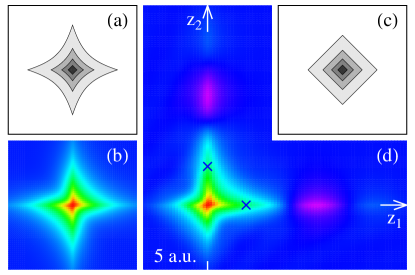
Figure 1: (Color online) The $x_{1}=y_{1}=x_{2}=y_{2}=0$ cut of the real part of: (a) the Chandrasekhar’s and (b) the numerically calculated ground state wave function of H^- (at $F=0$), (c) the wave function $\sim\exp[-a(r_{1}+r_{2})]$ representing a state with equivalent electrons, (d) the numerically calculated lowest state wave function of H^- in the electric field $F=0.03$ a.u. The crosses mark the positions of the barrier saddle points ($z_{\mathrm{sp}}\approx 3$ a.u.) estimated using the single-electron model (3).

The lowest state energies and widths (electron detachment rates) of H^- at different values of the applied electric field determined numerically using the two-electron model (1) are presented in Table 1 and in Fig. 2 together with the results obtained using other approaches. Fig. 2(a) shows that for weak fields the lowest state energy $E(F)$ (numerical data) decreases by increasing the field strength according to the Stark shift expansion formula $\Delta E\equiv E(F)-E(0)=-\alpha F^{2}/2!-\gamma F^{4}/4!-\cdots$. Here $E(0)=-0.5+E_{\mathrm{B}}=-0.5277$ a.u. is the ground state energy of the free ion, whereas $\alpha=206$ and $\gamma=8.03\cdot 10^{7}$ are the corresponding values of the dipole polarizability and the second dipole hyperpolarizability radzig ; pipin . At stronger fields ($F>0.01$), however, the lowest state energy depends on the field strength almost linearly. The same figure shows the results obtained using a single-electron model that will be discussed later.

As mentioned in the introductory part, the configuration of the ground state of H^- suggests a one-electron description where the outer (loosely bound) electron moves in a short-range potential $V(\mathbf{r})$ describing the attraction by the neutral atomic residue. Then, in the presence of a (quasi)static electric field $F$ the outer electron may be considered as moving in the total potential $V_{\mathrm{tot}}=V(\mathbf{r})-Fz$. $V(\mathbf{r})$ is usually calibrated to give the value $-E_{B}$ for the lowest energy level $\epsilon(F)$ at $F=0$. When $F\neq 0$ the total potential has a potential barrier that explains the resonant character of states. The saddle point of the barrier is located at the z-axis. Its position $\mathbf{r}_{\mathrm{sp}}=(0,0,z_{\mathrm{sp}})$ and hight $V_{\mathrm{sp}}=V_{\mathrm{tot}}(\mathbf{r}_{\mathrm{sp}};F)$ depend on the field strength $F$ and can be determined from the rule $(\partial V_{\mathrm{tot}}/\partial z)_{x=y=0}=0$. The field strength $F_{\mathrm{S}}$ that separates the tunneling and OBD regimes is defined by the condition $\epsilon(F_{\mathrm{S}})=V_{\mathrm{sp}}(F_{\mathrm{S}})$. Note that these values may vary by changing the model for $V(\mathbf{r})$.

Table 1: The lowest state energies $E$ and widths $\Gamma$ of the hydrogen negative ion at different strengths of applied electric field $F$, obtained by the complex rotation method within the single- and two-electron pictures. The single-electron calculations are performed using the CF potential (3).

	two-electron model		single-electron model
$\quad F\quad$	$-E$	$\Gamma$	$-E$	$\Gamma$
0	0.52763	0	0.52775	0
0.001	0.52773	-	0.52782	-
0.002	0.52814	-	0.52806	$7.330\!\cdot\!\!10^{-5}$
0.003	0.52867	$4.310\!\cdot\!\!10^{-4}$	0.52846	$4.511\!\cdot\!\!10^{-4}$
0.004	0.52928	$1.247\!\cdot\!\!10^{-3}$	0.52887	$1.091\!\cdot\!\!10^{-3}$
0.005	0.52997	$2.475\!\cdot\!\!10^{-3}$	0.52931	$1.913\!\cdot\!\!10^{-3}$
0.006	0.53057	$3.845\!\cdot\!\!10^{-3}$	0.52974	$2.933\!\cdot\!\!10^{-3}$
0.007	0.53118	$5.369\!\cdot\!\!10^{-3}$	0.53014	$4.122\!\cdot\!\!10^{-3}$
0.008	0.53177	$7.022\!\cdot\!\!10^{-3}$	0.53053	$5.335\!\cdot\!\!10^{-3}$
0.009	0.53236	$8.789\!\cdot\!\!10^{-3}$	0.53088	$7.034\!\cdot\!\!10^{-3}$
0.010	0.53293	0.01066	0.53121	$8.440\!\cdot\!\!10^{-3}$
0.011	0.53347	0.01258	0.53153	$9.872\!\cdot\!\!10^{-3}$
0.012	0.53397	0.01451	0.53182	0.01132
0.013	0.53451	0.01654	0.53214	0.01284
0.014	0.53503	0.01861	0.53240	0.01443
0.015	0.53559	0.02078	0.53265	0.01595
0.016	0.53609	0.02291	0.53289	0.01750
0.017	0.53660	0.02505	0.53313	0.01894
0.018	0.53708	0.02730	0.53336	0.02065
0.019	0.53762	0.02956	0.53360	0.02227
0.020	0.53817	0.03186	0.53376	0.02394
0.021	0.53864	0.03414	0.53399	0.02562
0.022	0.53915	0.03647	0.53422	0.02720
0.023	0.53965	0.03883	0.53441	0.02883
0.024	0.54016	0.04122	0.53454	0.03066
0.025	0.54071	0.04362	0.53473	0.03229
0.026	0.54120	0.04606	0.53492	0.03395
0.027	0.54170	0.04848	0.53512	0.03563
0.028	0.54222	0.05097	0.53525	0.03733
0.029	0.54274	0.05349	0.53538	0.03900
0.030	0.54320	0.05599	0.53556	0.04062

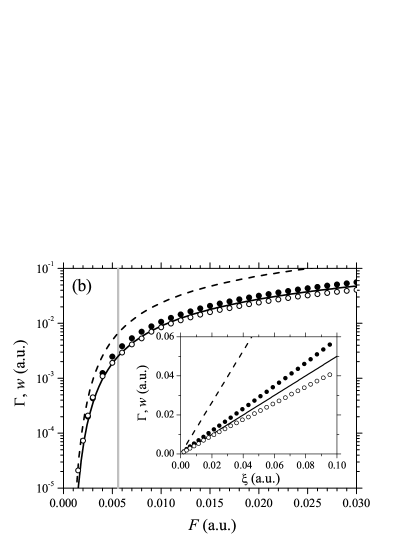
Figure 2: (a) The lowest state energy $E$ and (b) width $\Gamma$ (detachment rate $w$) of the hydrogen negative ion as functions of the strength of applied electric field $F$. The full and open circles denote the results obtained numerically using the two- and the single-electron CF (Eq. (3)) model, respectively. The dashed and full lines in part (a) show the lowest state energy $E(F)$ estimated using the second and the fourth order Stark shift formula, respectively. The dashed and full lines in part (b) show the rate $w(F)$ given by the PPT and the ZRP theory (Eq. (2) with $C_{\kappa}^{2}=1.32$ and $0.5$), respectively. The inset shows the same rates as functions of the variable $\xi$ (see text). Vertical gray lines separate the tunneling from OBD regime.

The first among the single-electron approaches we will consult is the Perelomov-Popov-Terent’ev (PPT) theory PPT . It is based on the quasistatic approximation and the assumption that most atoms are nearly hydrogenic, the difference being a small quantum defect that changes the quantum numbers to noninteger effective values. In the case of negative ions, however, the atomic residue is neutral ($Z=0$) and the effective principal quantum number $n^{*}=Z/\kappa$, where $\kappa=(2E_{\mathrm{B}})^{1/2}$, is equal to zero. Then the static-field tunneling rate formula for negative ions in the ground state reduces to

$$w=C_{\kappa}^{2}\frac{F}{\kappa}\exp\!\bigg{(}\!-\frac{2\kappa^{3}}{3F}\bigg{)}.$$ (2)

The coefficient in the pre-exponential factor for H^- determined from Hartree-Fock calculations has the value $C_{\kappa}=1.15$ popov . Fig. 2(b) shows that, although H^- does not belong to the class of hydrogenic atoms, the PPT rate formula exhibits a qualitative agreement with the numerical results.

It should be mentioned that the Ammosov-Delone-Krainov (ADK) theory ADK gives the same (genaral) formula for tunneling rates as the PPT theory, but in addition it provides an explicit expression for $C_{\kappa}$. This expression, however, is not useful in the case when $n^{*}=0$. The ADK theory, on the other hand, accurately predicts tunneling rates in experiments with atomic ionization in strong fields augst ; xiong and shows good agreement with available exact numerical results (for H and He see scrinzi ; themelis ). Even for atoms with low ionization potentials like alkali metals, using a correction which accounts for the Stark shift, the ADK tunneling rates agree well with numerical results MS . However, the non-Coulomb character of interaction between the neutral atomic residue and outer electron raise the question of applicability of the PPT or a similar theory to negative ions.

Regarding the latest discussion we can expect a better agreement between the single- and the two-electron approach if in the former we apply a short-range potential. As mentioned above, the simplest short-range potential that can be used to describe the dynamics of a weakly bound electron in negative ions is the ZRP: $V(\mathbf{r})=-a\delta(\mathbf{r})$ ($a>0$). This potential supports only one bound state whose wave function has the form $\psi(\mathbf{r})\sim\exp(-\kappa r)/r$, where $\kappa\equiv(2E_{\mathrm{B}})^{1/2}=a$ dem-ost . The eigenvalue problem of the single-electron Hamiltonian with $V_{\mathrm{tot}}=-a\delta(\mathbf{r})-Fz$ admits for weak fields a solution in a closed analytical form dem-ost . The lowest state energies and widths are represented by the Stark shift expansion with the polarizability $\alpha=1/(16E_{\mathrm{B}}^{2})\approx 81.5$ and by Eq. (2) with $C_{\kappa}^{2}=1/2$. Hence, the PPT and ZRP rate formulae differ only by the value of constant $C_{\kappa}$.

The exact value of constant $C_{\kappa}$ can be obtained by fitting the numerical results obtained applying the two-electron model. For this purpose we express the rate in terms of the variable $\xi=(F/\kappa)\exp(-2\kappa^{3}/(3F))$. Then the rate formula (2) reduces to the linear dependence $w=C_{\kappa}^{2}\xi$. It is found that the numerical data fits well to Eq. (2) for $C_{\kappa}^{2}=0.585\pm 0.010$ (see the inset in Fig. 2(b)).

Finally we consider the single-electron model for H^- where the loosely bound electron moves in an effective potential that is the sum of a short-range potential and the polarization term. A widely used potential of this type is the Cohen-Fiorentini (CF) potential CF

$$V=-\bigg{(}1+\frac{1}{r}\bigg{)}e^{-2r}-\frac{\alpha_{\mathrm{H}}}{2r^{4}}\,e^{-r_{0}^{2}/r^{2}},$$ (3)

where $\alpha_{\mathrm{H}}=9/2$ is the polarizability of the hydrogen atom. The parameter $r_{0}=1.6$ is chosen by the condition that the potential (3) has a single bound state with the correct binding energy. The lowest state energies [$E(F)=\epsilon(F)-0.5$ a.u.] and widths of the H^- in (quasi)static electric field, obtained using the CF potential, are shown in Table 1 and Fig. 2. The calculations were performed using the complex rotation method reinhardt ; buchleitner and Sturmian basis avery .

At low values of $F$ the energies obtained by the latest model approximately agree with the two-electron (exact) results (see Fig. 2(a)). At stronger fields, however, the difference between these results increases, particularly in the OBD area. The value of $F$ that separates the tunneling and OBD regimes obtained using the potential (3) is $F_{\mathrm{S}}=0.0056\pm 0.0001$. For $F>2F_{\mathrm{S}}$ the exact Stark shift $\Delta E_{\mathrm{2e}}$ is approximately two times larger than $\Delta E_{\mathrm{1e}}$ obtained using the single-electron approach (the uncertainty in $F_{\mathrm{S}}$ is due to this difference). The rates determined using the CF single-electron model agree with the two-electron results approximately for $F<F_{\mathrm{S}}/2$, see Fig. 2(b). Otherwise the single-electron calculations underestimate the two-electron results (for about 30$\%$ in the OBD regime).

These differences indicate that the single-electron picture is not valid at stronger fields. At the field strengths $F\sim F_{\mathrm{S}}$ the potential barrier is suppressed enough that the lowest state cannot be treated as bound even approximately. In this case the Chandrasekhar’s concept of outer electron is not adequate because a significant part of the probability distribution lies at the outer side of barrier ($z>z_{\mathrm{sp}}$). In other words the ’outer’ electron becomes the ’outgoing’ electron. Simultaneously, the form of the two-electron wave function in the inner region ($z<z_{\mathrm{sp}}$) becomes more similar to that for equivalent electrons (see Fig. 1(c,d)), that explains the failure of single-electron approach (particularly for energies). The ratio $\Delta E_{\mathrm{2e}}/\Delta E_{\mathrm{1e}}\approx 2$ for $F\gg E_{\mathrm{S}}$ may be explained by the fact that in the states of this form the shift $\Delta E_{\mathrm{2e}}$ includes the contributions of both electrons.

In conclusion, the single-electron description of the lowest state of H^-, that is a good approximation in the field-free and low-field cases, fails in OBD and partially in the tunneling regime. This is important to know because single-electron models are often used to study negative ions in strong fields. We determined the exact lowest state energies and detachment rates for H^- at different strengths of the applied (quasi)static field by solving the eigenvalue problem of the full two-electron Hamiltonian. The PPT and ZRP theories lead to the same rate formula, but with different values of the constant in the pre-exponential factor. The accurate value of the constant is obtained by fitting the numerical results determined using the two-electron model.

This work is supported by the COST Action CM1204 (XLIC). N. S. S. acknowledges support by the Ministry of education, science and technological development of Republic or Serbia under Project 171020.

References

- (1) H. A. Bethe, 1929, Z. Phys. 57, 815 (1929).
- (2) A. R. P. Rau, J. Astrophys. Astr. 17, 113 145 (1996).
- (3) T. Andersen, Phys. Rep. 394, 157 (2004).
- (4) T. Andersen, H. K. Haugen and H. Hotop, J. Phys. Chem. Ref. Data 28, 1511 (1999).
- (5) K. R. Lykke, K. K. Murray, and W. C. Lineberger, Phys. Rev. A 43, 6104 (1991)
- (6) A. A Radzig and B. M. Smirnov, Reference Data on Atoms, Molecules and Ions (Springer-Verlag, Berlin, 1985), p. 119, 131.
- (7) S. Chandrasekhar, Astrophys. J. 100, 176 (1944).
- (8) P. V. Grujić and N. Simonović, J. Phys. B: At. Mol. Opt. Phys. 31, 2611 (1998).
- (9) Yu. N. Demkov and V. N. Ostrovskii, Zero-range potentials and their applications in atomic physics (Plenum Press, New York, 1988).
- (10) R. Wildt, Astrophys. J. 89, 295 (1939).
- (11) H. C. Bryant, M. Halka, in Coulomb Interactions in Nuclear Atomic Few-Body Collisions, eds. F. S. Levin and D. A. Micha (Plenum Press, New York, 1996) p. 221.
- (12) L. V. Keldysh, Sov. Phys. JETP 20, 1307 (1965).
- (13) W. P. Reinhardt, Int. J. Quant. Chem. Symp. 10, 359 (1976).
- (14) A. Buchleitner, B. Grémaud and D. Delande, J. Phys. B: At. Mol. Opt. Phys. 27, 2663 (1994).
- (15) J. Avery and J. Avery, Generalized Sturmians and Atomic Spectra (Singapore: World Scientific, 2006).
- (16) J. Pipin and D. M. Bishop, J. Phys. B: At. Mol. Opt. Phys. 25, 17 (1992).
- (17) A. M. Perelomov, V. S. Popov, and M. V. Terent’ev, Sov. Phys. JETP 23, 924 (1966).
- (18) V. S. Popov, Physics – Uspekhi 47, 855 (2004).
- (19) M. V. Ammosov, N. B. Delone, and V. P. Krainov, Sov. Phys. JETP 64, 1191 (1986).
- (20) S. Augst, D. D. Meyerhofer, D. Strickland, and S. L. Chin, J. Opt. Soc. Am. B 8, 858 (1991).
- (21) W. Xiong and S. L. Chin, Sov. Phys. JETP 72, 268 (1991).
- (22) A. Scrinzi, M. Geissler, and T. Brabec, Phys. Rev. Lett. 83, 706 (1999).
- (23) S. I. Themelis, T. Mercouris, and C. A. Nicolaides, Phys. Rev. A 61, 024101 (1999).
- (24) M. Z. Milošević and N. S. Simonović, Phys. Rev. A 91, 023424 (2015).
- (25) J. S. Cohen and G. Fiorentini, Phys. Rev. A 33, 1590 (1986).