Abstract

Transient premixed hydrogen/air flames contracting through inhomogeneous fuel distributions and subjected to stretch and pressure oscillations are investigated numerically using an implicit method which couples the fully compressible flow to the realistic chemistry and multicomponent transport properties. The impact of increasing negative stretch is investigated through the use of planar, cylindrical and spherical geometries, and a comparison with the results from positively stretched expanding H2/air flames ([Malik and Lindstedt (2010)]) and CH4/air flames ([Malik and Lindstedt (2012)]) is made. A flame relaxation number $n_{R}=\tau_{R}/\tau_{L}$ ($\tau_{R}$ is the time that the flame takes to return to the mean equilibrium conditions after initial disturbance; $\tau_{L}$ is a flame time scale) decreases by 10% with increasing negative stretch, in contrast to the two expanding flames where $n_{R}$ decreased by 40% with increasing positive stretch. $n_{R}$ appears to much more sensitive to variations in positive/negative curvature than to the thermo-chemistry of different flame types. $n_{R}$ may thus be a useful indicator of the strength of flame-curvature coupling. The spectra of pressure fluctuations $E_{p}(\omega)$ scale close to $\sim\omega^{-3}$, which is steeper than in the expanding H2/air flames where $E_{p}(\omega)\sim\omega^{-2}$. Rapid transport (’flapping’) of the flame front by the largest convective velocities induced by the random pressure fluctuations is prominent because of the lack of gas velocity ahead of the flame, $u_{g}=0$. ’Memory effects’ between fuel consumption and the rate of heat release is obscured by the flapping, although the contracting flames display short time-lags in the mean. A spectrum of species thickness $\{l_{k}\}$ exists such that species formed in thin reaction layers are generally not disturbed except with respect to their peak concentration, and species formed in thick reaction layer are disturbed along their entire length.

PACS numbers: 47.27.E?, 47.27.Gs, 47.27.jv, 47.27.Ak, 47.27.tb, 47.27.eb, 47.11.-j

keywords: flame;premixed; pressure fluctuations; stretch; flame velocity; chemical kinetics; curvature;multicomponent transport; methane; direct simulations; implicit.

1 Introduction

Most naturally occurring flames are turbulent and unsteady and occur in the presence of significant local stretch. Furthermore, The response of the flame kernel to pressure fluctuations can lead to violent amplification of the heat release, while lean gas mixtures can be difficult to ignite and sustain, with the possible consequence of self-induced oscillations. The coupling between the flame structure and the unsteady flow field is therefore of fundamental importance both to the theory of flames and to practical combustion systems.

But direct measurements of the local flame structure and its response to stretch has proved difficult. As a consequence cylindrically and spherically symmetrical flames have often been studied because these geometries provide simplifications from which information regarding fundamental aspects of flames can still be extracted.

Outwardly propagating flames occur widely such as in automotive engines where fuel/air mixtures are ignited inside a cylinder under high pressure to form a small approximately spherical expanding flame that releases heat to produce useful work, as seen in the images inside an engine captured by [Heywood (1988)]. Expanding flames have been studied more often than implosions as they are easier to produce experimentally; They have been studied experimentally by [Dowdy (1990), Taylor (1991), Kown et al (1992), Tseng et al (1993), Karpov et al (1997)), Kelley and Law (2009)] and numerically by [Bradley et al (1996), Malik and Lindstedt (2010)] and [Malik (2012)].

Inwardly propagating flames are important because they are not subject to strain due to the zero gas velocity ahead of the flame, and stretch is therefore due to the curvature alone and so the effects of curvature can be studied in isolation. This is important because curvature can have a dominant effect in many combustion phenomena as well as in other powerplant flows, see for example [Korakianitis (1993), Korakianitis and Papagiannidis (1993), Korakianitis et al (2007), Pachidis et al (2006), Hamakhan and Korakianitis (2010)]. Experimentally, implosions are difficult to produce and little data is available; exceptions though are the experiments of al [Baillot et al (2002)] and [Groot and De Goey (2002)]. Imploding methane/air flames have been investigated numerically by  [Bradley et al (1996)],  [Kelley and Law (2009)] and [Malik (2012)].

The last twenty years have seen great progress in the understanding of flame interactions with physical oscillations of different types. Quite often models are adopted with approximations in the modeling of the flow and/or the chemistry, e.g. 1-step chemistry, [Teerling et al (2005)]; parametric variations in only one physical variable such as the equivalence ratio [Marzouk et al (2000), Sankaran and Im (2002)], induced pressure fluctuations, [Teerling et al (2005)], harmonic velocity fluctuation, [Lieuwen (2005)], and flame response to unsteady strain and curvature have also been explored, [Najm and Wyckoff (1997)]. The impact of pressure fluctuations upon combustor stability have been highlighted in a number of studies e.g. [Candel (2002), Luff (2006)], and there is evidence that the intrinsic thermochemical structure may lead to pulsating instabilities, [Christiansen and Law (2002), Gummalla and Vlachos (2000), Lauvergne and Egolfopoulos (2000))]. Large Eddy Simulations with a flame surface density model has been used to investigate expanding flames, [Ibrahim et al (2009)].

Most of the studies noted above focus on particular effects in isolation, but there is also a need to examine more complex situations where many unsteady processes are occurring at the same time, which is closer to reality. Therefore, in this study we investigate the combined effect of simultaneous fluctuations in pressure and fuel concentration in unsteady finite thickness flames.

Although major advances in computer simulations of combustion systems have been made in recent years, detailed computational studies are still comparatively few, e.g. [Bradley et al (1996), Lindstedt et al (1998), Meyer (2001), Korakianitis et al (2004), Dyer and Korakianitis (2007), Malik and Lindstedt (2010), Malik (2012)]. With the need to interrogate complex reacting systems in greater detail, it is recognised that a step forward in computational combustion requires the inclusion of more realistic chemistry coupled to the compressible flow, as highlighted in [Lu and Law (2009), Malik and Lindstedt (2010), Malik and Lindstedt (2012), Malik (2012)].

The need for the inclusion of realistic chemistry is especially important in view of the need to predict emissions of green-house gasses and particulates from industrial devices with a fair degree of accuracy and reliability, as noted by [Løvås et al (2010)]. New challenges are related to the yet unknown behaviour of alternative fuels, such as bio-fuels. Although overall green-house gas emissions are low for biomass fuels, these fuels emit higher concentrations of heavy metals and particulates which can be a hazard to industrial devices, such as in automotive engines where the role played by differential diffusion in species and particle transport is of special concern, [Løvås et al (2010), Mauss et al (2006), Marchal et al (2009)].

The recent progress in numerical software and in computer technology now offers the possibility to couple the detailed chemistry to the compressible flow. Large Eddy Simulations are the methods of choice in large scale numerical simulations in practical applications because they provide an acceptable compromise between grid resolution and the overall size of the system, e.g. [Malalasekera et al (2008)] investigate recirculation and vortex breakdown of swirling flames using LES, and Luo et al have used LES to investigate interactions between a reacting plume and water spray, [Xia et al (2008)], and the aeroacoustics of an unsteady three-dimensional compressible cavity flow, [Lai et al (2007)].

At a more fundamental level, Direct Numerical Simulations using explicit methods have matured in the last fifteen years and are providing useful data, [Thévenin et al (2002), Chakraborty and Cant (2004), Jiang et al (2007), Lignell et al (2008), Schroll et al (2009), Chen et al (2006), Gou et al (2010)]. Although they have had stability problems, significant progress has been made recently in chemical stiffness removal and multi-dimensional scale integration in the studies mentioned above. Nevertheless, it is common practice to use reduced chemical schemes in these codes in order to improve stability.

Implicit methods have been receiving some attention recently as they are well known to provide stable solvers even for stiff systems although at the cost of large memory requirements. Smooke and co-workers have developed implicit compact scheme solvers for 2D non-reacting flows, [Noskov et al (2007)], and for 1D reacting flows with simplified global reaction source term, [Noskov and Smooke (2005)]. Malik has developed an implicit finite volume method, TARDIS (Transient Advection Reaction Diffusion Implicit Simulations), [Malik and Lindstedt (2010), Malik and Lindstedt (2012), Malik (2012)], featuring the coupling of the compressible flow to the comprehensive chemistry and the detailed multicomponent transport properties of the mixture, thus resolving all the convective and chemical length and time scales which is essential for studying stiff and unsteady reacting systems.

TARDIS thus provides a platform for studying in detail regimes of combustion which were previously difficult to explore due to the limitations of experimental and other numerical methods; for example, unsteady combustion processes in automobile engines have not been explored numerically or experimentally with full chemistry. One of the main purposes of this work is to deomstrate the capability of TARDIS to such complex systems.

An area of special interest in this study is the regime of relatively high Karlovich number $K=\kappa\tau_{L}\geq 1$, where $\kappa=A^{-1}dA/dt$ is the stretch, the rate of change of an elemental area $A(r)$ surrounding a point on the surface of the flame, and $\tau_{L}$ is a flame time scale. In this limit, the convective fluctuations can penetrate inside the internal structure of the flame thus disturbing the flame structure and the system is then essentially unsteady. Little is known of the flame response in this limit and yet its occurrence is widespread because most combustion occurs under turbulent conditions, such as in internal combustion engines, when the smaller convective scales are able to penetrate inside the flame kernel. Many models of turbulent flames often assume that the turbulent flame front consists of a collection of laminar flamelets so that the steady laminar flame structure is assumed to remain undisturbed. But clearly such an assumption cannot remain valid when the convective scales penetrate inside the flame kernel.

The aim of this work is two-fold. First, we use TARDIS to study stoichiometric hydrogen/air inwardly propagating flames (implosions) in cylindrical and spherical geometries at mean atmospheric pressure – essentially small fuel pockets being consumed. We explore the coupling of the thermochemical flame structure to pressure oscillations in the context of inhomogeneous fuel distributions and for different levels of negative stretch (flow divergence), and how this affects properties of the flame such as the flame speed and flame structure.

Second, the results will be compared to the results from [Malik and Lindstedt (2010), Malik and Lindstedt (2012)] who carried out related studies on expanding hydrogen/air and methane/air flames.

2 Inwardly propagating flames

Inwardly propagating flames have not been studied as much as expanding flames because they are difficult to produce experimentally. Exceptions though are [Baillot et al (2002)] and [Groot and De Goey (2002)]; Baillot et al produced small spherical bubbles of methane-air about 1 mm diameter (which have high curvature). Numerical simulations of imploding flames are also scarce; [Bradley et al (1996)] investigated the methane/air system using a simplified 4-step mechanism and a simplified set of balance equations in which the momentum equation was neglected under the assumption that pressure gradients were negligible; and [Malik (2012)] has investigated stretched flame velocities in different geometries for different fuels and modes of propagation.

Inwardly propagating laminar flames are not subject to strain due to the zero velocity ahead of the flame. Stretch is therefore due to the curvature alone and so the effects of curvature can be studied in isolation.

A flame front velocity $u_{f}$ is defined as the physical movement of the flame in space, and is given by the sum of the burning velocity $s_{n}$ and the gas velocity $u_{g}$, $u_{f}=s_{n}+u_{g}$. In the case of inwardly propagating flames where $u_{g}=0$ ahead of the flame in the fresh gas mixture, we have $u_{f}=s_{n}$. In the current study, there is a third component $u^{\prime}_{p}$ induced by the pressure fluctuations, thus $u_{f}=s_{n}+u^{\prime}_{p}$ ahead of the flame. Note that the pressure fluctuations exist throughout the domain and therefore $u^{\prime}_{p}$ can be non-zero anywhere in the domain, even ahead of the flame where the velocity is usually expected to be zero.

3 Method

The current study features an implicit method, TARDIS (see [Malik and Lindstedt (2010), Malik and Lindstedt (2012), Malik (2012)]), in which the balance equations of mass, momentum, energy and chemical species, together with the state equation for ideal gas, are solved in an implicit framework on a staggered grid arrangement. The governing balance equations are functions of time, $t$, and one spatial coordinate, $x$ or $r$ (radius), only. The governing equations are,

$$\displaystyle{{\partial\rho}\over{\partial t}} +\displaystyle{1\over r^{\alpha}}{{\partial r^{\alpha}\rho u}\over{\partial r}} =0$$ (1)

$$\displaystyle{{\partial\rho u}\over{\partial t}} +\displaystyle{1\over r^{\alpha}}{{\partial r^{\alpha}\rho u^{2}}\over{\partial r}} =-\displaystyle{1\over r^{\alpha}}{{\partial r^{\alpha}J_{\nu}}\over\partial r}-\displaystyle{{\partial P}\over\partial r}+\chi^{\alpha}$$ (2)

$$\displaystyle{{\partial\rho e}\over{\partial t}} +\displaystyle{1\over r^{\alpha}}{{\partial r^{\alpha}\rho ue}\over{\partial r}} =-\displaystyle{1\over r^{\alpha}}{{\partial r^{\alpha}J_{e}}\over\partial r}$$ (3)

$$-\sum_{k=1}^{N}\displaystyle{{1\over r^{\alpha}}{{\partial}\over\partial r}[r^{\alpha}h_{k}(-J_{k}+J_{n})]}$$

$$+{P\over r^{\alpha}}\displaystyle{{\partial r^{\alpha}u}\over{\partial r}}+\Gamma^{\alpha}+\mu\Psi^{\alpha}$$

$$\displaystyle{{\partial\rho Y_{k}}\over{\partial t}} +\displaystyle{1\over r^{\alpha}}{{\partial r^{\alpha}\rho uY_{k}}\over{\partial r}}= -\displaystyle{1\over r^{\alpha}}{{\partial r^{\alpha}J_{k}}\over\partial r}+\dot{R}_{k}W_{k}$$ (4)

$$P =\displaystyle{{\rho RT}\over W}$$ (5)

where $\alpha=0$ for planar flames; $\alpha=1$ for cylindrical flames; $\alpha=2$ for spherical flames. $\rho$ is the density, $u$ is the velocity, $P$ is the pressure, $e$ is the internal energy, $Y_{k}$ are the species mass fractions for $k=1,...,N$ species, $\dot{R}_{k}$ is the molar rate of production of the $k^{th}$ species, $t$ is the time, $T$ is the temperature, $W$ is the mean molecular mass, $W_{k}$ is the molecular mass of the $k^{th}$ species, $J_{\nu}$ is the viscous flux of momentum, $J_{e}$ is the energy flux, $J_{k}$ is the $k^{th}$ species diffusive flux, $J_{n}$ is the flux of heat and $R$ is the gas constant.

For all flame geometries ($\alpha=1,2,3$):

$\chi^{\alpha}=-\alpha\left(\displaystyle{{{2u}\over 3r}{{\partial\mu}\over{\partial r}}}\right)$, and $\Gamma^{\alpha}=\displaystyle{{1\over r^{\alpha}}{\partial\over{\partial r}}}\left(\displaystyle{r^{\alpha}{{\lambda RT}\over C_{v}}{\partial\over{\partial r}}\left({1\over W}\right)}\right)$

For planar flames:
$\Psi^{0}=\displaystyle{{4\over 3}({{\partial u}\over{\partial r}})^{2}}$.

For cylindrical flames:
$\Psi^{1}=\displaystyle{{4\over 3}\left({{\partial u}\over{\partial r}}-{u\over r}\right)^{2}+{4\over 3}\left({u\over r}{{\partial u}\over{\partial r}}\right)}$

For spherical flames $\Psi^{2}$ has the same form as $\Psi^{1}$ except that the last term is absent.

Models for the various fluxes are given by,

$$J_{\nu} = -\displaystyle{4\over 3}\mu\displaystyle{{\partial u}\over{\partial r}}$$ (6)

$$J_{k} = -\rho D_{k}\left(\displaystyle{{{\partial Y_{k}}\over{\partial r}}-\displaystyle{Y_{k}\over n}{{\partial n}\over{\partial r}}}\right)+\rho\Theta_{k}Y_{k}+\rho V_{c}Y_{k}\qquad k=1,2,...,N$$ (7)

$$J_{e} = -\displaystyle{\lambda\over C_{v}}\displaystyle{{\partial e}\over{\partial r}}$$ (8)

$$J_{n} = -\displaystyle{\lambda\over C_{v}}\displaystyle{{\partial Y_{k}}\over{\partial r}}$$ (9)

$\mu$ is the dynamic viscosity, $\lambda$ is the thermal conductivity, $n$ is the mole number, and $C_{v}$ is the specific heat capacity at constant volume.

Viscosities and binary diffusivities are evaluated using the theory of Chapman & Enskog (see [Reid and Sherwood (1960))]), Thermal conductivities from [Mason and Monchick (1962)]. Mixture properties are evaluated from Wilkes formula (see [Reid and Sherwood (1960))]). The diffusive fluxes include the Soret thermal–diffusion for light species ($H$ and $H_{2}$).

Thus, all transport properties are evaluated locally and are functions of the local temperature, which allows the system to be strongly inhomogeneous in transport properties and gives the simulations an added degree of reality. The specific Lewis numbers are, therefore, non-unity, $Le_{k}=Le_{k}(T)$, and functions of the local temperature as well.

The same transport relations above are used in all of the simulations, and flame speeds are calculated using an integral definition, equation (4.1).

The chemistry is modeled as a detailed system containing $N$ chemical species, in $N_{r}$ elementary reactions, whose reaction rates are given by,

$$\dot{R}_{k} = \sum_{j=1}^{N_{r}}(\nu^{{}^{\prime\prime}}_{kj}-\nu^{{}^{\prime}}_{kj})\left[{k_{j}^{f}\prod_{l=1}^{N}\phi_{l}^{\nu^{{}^{\prime}}_{jl}}-k_{j}^{r}\prod_{l=1}^{N}\phi_{l}^{\nu^{{}^{\prime\prime}}_{jl}}}\right]$$ (10)

where $\phi_{l}$ is the molar concentration of the $l^{th}$ chemical species, and $\nu^{{}^{\prime}}$ and $\nu^{{}^{\prime\prime}}$ are the stoichiometric coefficients of reactants and products respectively. The forward reaction rate constant in reaction number $j$ is given by Arrhenius’ law,

$$k_{j}^{f} = A_{j}T^{\beta_{j}}\exp({-\Delta E_{j}/RT})$$ (11)

The hydrogen/air chemistry, shown in Table 1, is a comprehensive system featuring 9 species and 30 reactions where the constants $A_{j}$, $\beta_{j}$ and the energy barrier $\Delta E_{j}$ were obtained from [Sun et al (2007)], with some modifications as noted in [Malik and Lindstedt (2010)]. Thermodynamic data were computed using JANAF polynomials.

Table 1. Detailed H₂/O₂ Reaction Mechanism with rate coefficients in the form $k=AT^{n}exp(-E/RT)$^a from Sun et al. (2007). The rate proposed by Sutherland et al. (1986) was used for reaction (2).

Number	Reaction		$A^{\rm a}$	$n^{\rm a}$	$E^{\rm a}$
1	H + O2 $\rightleftharpoons$ O + OH		6.73E+12	-0.50	69.75
2	O + H2 $\rightleftharpoons$ H + OHb		5.08E+01	2.67	26.33
3	H2 + OH $\rightleftharpoons$ H2O + H		2.17E+05	1.52	14.47
4	Oh + OH $\rightleftharpoons$ O + H2O		3.35E+01	2.42	-8.06
5	H2 + M $\rightleftharpoons$ H + H + Mc		2.23E+11	0	40.196
	H2 + H2$\rightleftharpoons$ H + H + H2		9.03E+11	0	40.196
	H2 + N2 $\rightleftharpoons$ H + H + N2		4.58E+16	-1.40	43.681
	H2 + H2O $\rightleftharpoons$ H + H + H2O		8.43E+16	-1.10	43.681
6	O + O + M $\rightleftharpoons$ O2 + Md		6.16E+09	-0.5	0.0
7	O + H + M $\rightleftharpoons$ OH + Md		4.71E+12	-1.0	0.0
8	H + OH + M $\rightleftharpoons$ H2O + Me		2.21E+16	-2.0	0.0
9	O2 + H (+ M) $\rightleftharpoons$ HO2 (+ M)f	$k_{0}$	2.65E+13	-1.30	0.0
		$k_{\infty}$	4.65E+09	0.4	0.0
	O2 + H (+ H2O) $\rightleftharpoons$ HO2 (+ H2O)g	$k_{0}$	3.63E+13	-1.00	0.0
		$k_{\infty}$	4.65E+09	0.4	0.0
10	H2 + O2 $\rightleftharpoons$ HO2 + H		7.40E+02	2.43	223.85
11	HO2 + H $\rightleftharpoons$ OH + OH		6.00E+10	0	1.23
12	HO2 + O $\rightleftharpoons$ OH + O2		1.63E+10	0	-1.86
13	HO2 + OH $\rightleftharpoons$ H2O + O2b		1.00E+10	0	0.00
			5.80E+10	0	16.63
14	HO2 + HO2 $\rightleftharpoons$ H2O2 + O2b		4.20E+11	0	50.133
			1.30E+08	0	-6.817
15	H2O2 (+ M) $\rightleftharpoons$ OH + OH (+ M)h	$k_{0}$	1.2E+14	0	190.37
		$k_{\infty}$	3.00E+14	0	202.84
16	H2O2 + H $\rightleftharpoons$ H2O + OH		1.02E+10	0	14.96
17	H2O2 + H $\rightleftharpoons$ H2 + HO2		1.69E+09	0	15.71
18	H2O2 + O $\rightleftharpoons$ OH + HO2		8.43E+08	0	16.61
19	H2O2 + OH $\rightleftharpoons$ H2O + HO2b		1.70E+15	0	123.05
			2.00E+09	0	1.79
20	HO2 + H $\rightleftharpoons$ H2O + O		1.44E+09	0	0

^aUnits are kmole, m³, s, K and KJ/mole.

^bReactions (13), (14) and (19) are expressed as the sum of the two rate expressions.

^cChaperon efficiencies are 0.0 for H₂, H₂O, N₂ and 1.0 for all other species.

^dChaperon efficiencies are 2.5 for H₂, 12.0 for H₂O and 1.0 for all other species.

^eChaperon efficiencies are 2.5 for H₂, 6.39 for H₂O and 1.0 for all other species.

^fTroe parameter is F_c=0.57. Chaperon efficiencies: 1.49 for H₂, 0.0 for H₂O and 1.0 for other species.

^gTroe parameter is F_c=0.81. Chaperon efficiencies: 1.0 for H₂O and 0.0 for other species.

^hTroe parameter is F_c=0.50. Chaperon efficiencies: 2.5 for H₂, 12.0 for H₂O and 1.0 for other species.

The pressure field consists of a mean and a fluctuating components, $p=\langle p\rangle+p^{\prime}$; similarly for the velocity $u=\langle u\rangle+u^{\prime}_{p}$. Transmissive (non-reflecting) boundary conditions were imposed on the mean pressure and mean velocity at the open (outer) boundary, but the fluctuating quantities $p^{\prime}$ and $u^{\prime}_{p}$ were reflected back in to the domain, which sustains the fluctuations inside the domain for long periods. For the curved flames we have $u=0$ at the centre ($r=0$). For details of the simulation method and validation, see Malik and Lindstedt (2010, 2012)

In order to simulate conditions inside practical devices such as engines, it is desirable to produce unforced pressure fluctuations subject to natural decay due to the action of viscosity, which is typical of conditions after ignition in an engine. This was achieved by running a pre-calculation consisting of releasing a set of square pressure ramps of large amplitude inside a domain of length $L$; these pressure ramps then diffuse, convect and reflect back from the ends of the domain until random pressure fluctuations of small amplitude with a range of frequencies are obtained. When the fluctuations have decayed down to a suitable level (about $2\%$ of atmospheric pressure), the main simulations were started ($t=0$) by introducing the fuel inhomogeneity as a sinusoidal oscillation cycle in the equivalence ratio just ahead of the flame front, $\phi(r)=1.0+A_{\phi}\sin(2\pi r/\lambda_{\phi})$, where $\lambda_{\phi}$ is the length scale of variation and $A_{\phi}$ is the initial amplitude. Four cases of moderate inhomogeneity $A_{\phi}\ll 1$ were consider, $A_{\phi}=-0.2,-0.1,0.1,0.2$.

A domain size of $L=400mm$ was found to produce pressure oscillations in the required frequency range $200-1000$Hz which are known to couple to the flame thermo-chemistry.

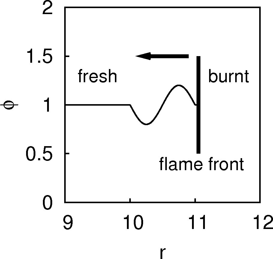
Figure 1: Schematic of the start of the simulations, showing the equivalence ratio $\phi$ against the radius $r$. The flame propagates from right to left into the inhomogeneous fuel distribution. (Pressure fluctuations are also active in the domain)

Figure 1 shows a schematic of the situation just as the flame is about to propagate into the equivalence ratio oscillation cycle. Figure 2 shows typical snapshots of (a) the pressure field and (b) the associated velocity field across the H2/air cylindrical flame at some instant. The non-zero velocity observed ahead of the flame is induced by the pressure fluctuations which exist throughout the domain. The location of the flame front is indicated by the vertical dashed lines in Figure 2 – one can observe the jump in velocity due to the gas expansion behind the flame.

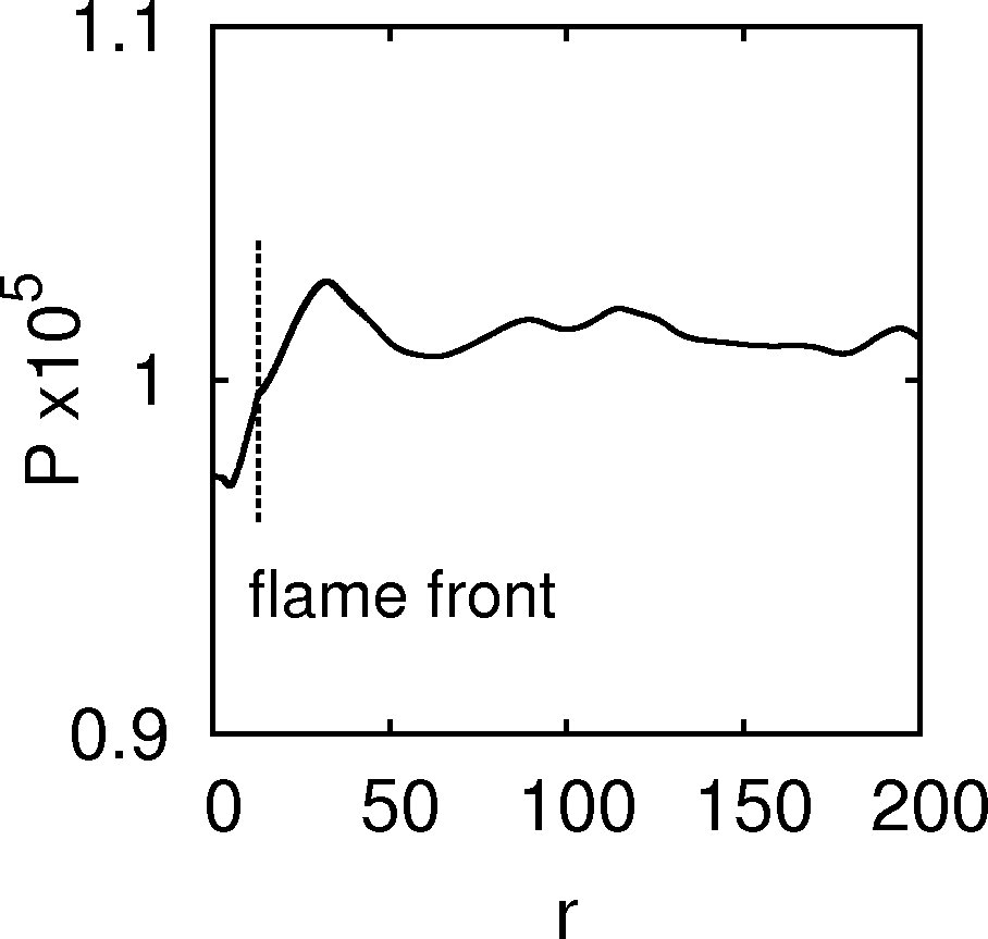
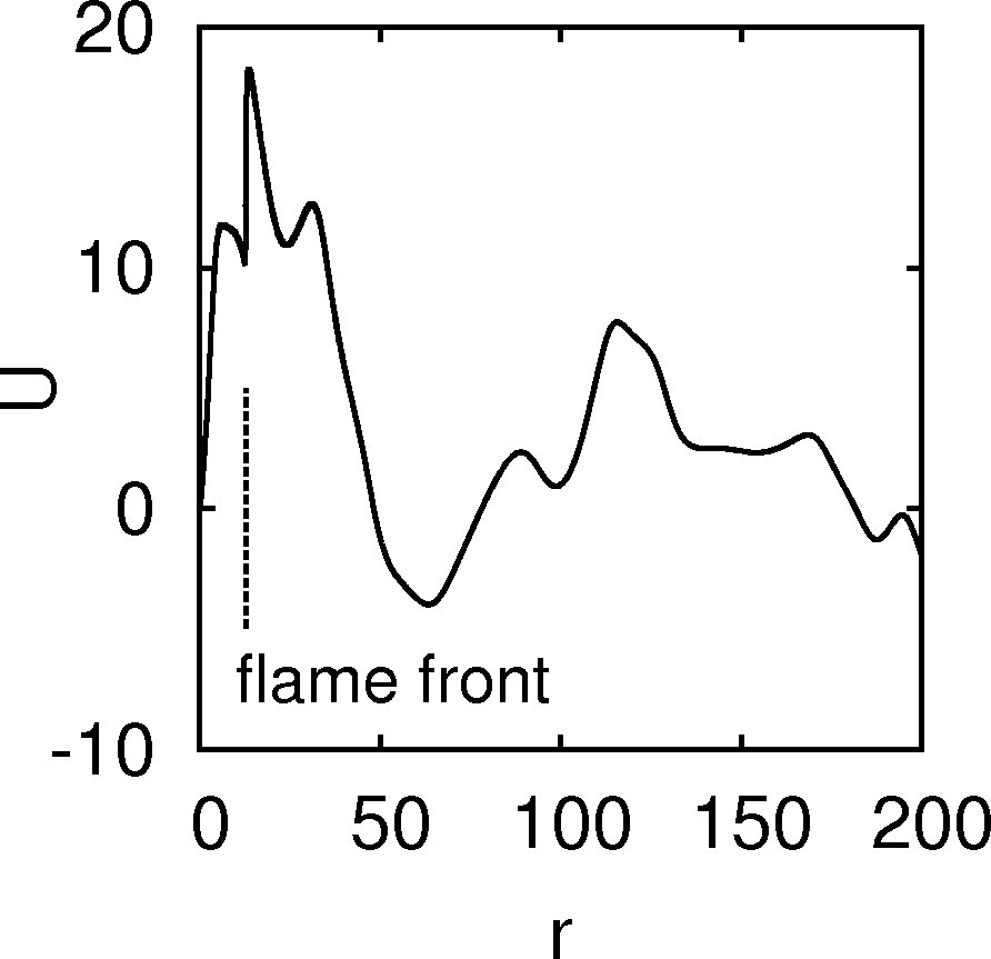
Figure 2: Left: The pressure field and, Right: the velocity field across a $200$ mm section of the domain taken from a typical simulation of a cylindrical flame. The vertical dashed lines indicate the location of the flame front

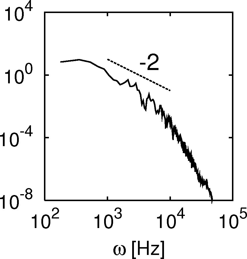
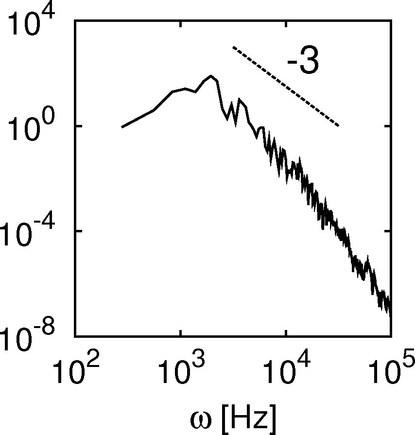
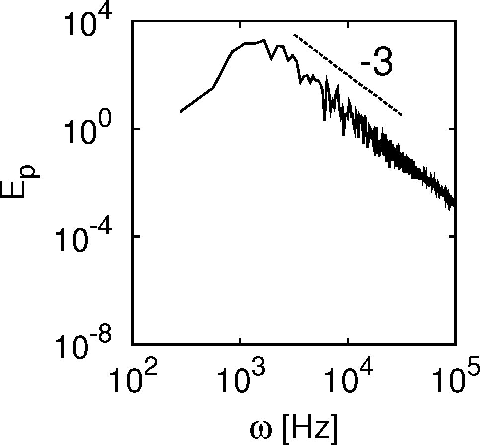
Figure 3: Log–log spectra of pressure fluctuations $E_{p}$, normalised by $E_{p}(0)$, against the frequency $\omega$ [Hz]: top left: Planar flame, top right: Cylindrical flame, bottom: Spherical flame

4 Results

4.1 Pressure Spectra

Pressure signals were recorded at points close to the flame fronts, spaced sufficiently far so as to avoid duplicate signals, yielding a total of five peridograms from which the final spectra were obtained by averaging. The signals were initially subjected to smoothing using a cubic spline solver on to 4096 point signal. Figure 3 shows the pressure spectra $E_{p}(\omega)$ in log-log scale from the flame simulations: 3(b) from the cylindrical flame, and 3(c) from the spherical flame, and for comparison the spectrum from the planar flame figure 3(a) from [Malik and Lindstedt (2010)] is also included. All spectra are normalised by $E_{p}(0)$. The spectra is an indicator of the strength of flame response to pressure fluctuations. Stronger flame-pressure interaction should produce a shallower gradient in the spectral broadening. In the case of high frequency pressure forcing which are known not to interact with the flame kernel, the spectrum falls off very steeply (as seen in Figure 4 in [Malik and Lindstedt (2010)]).

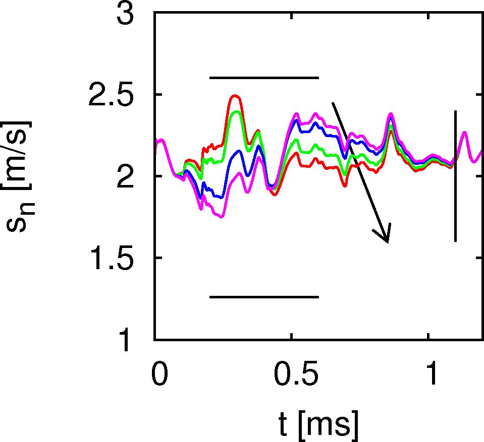
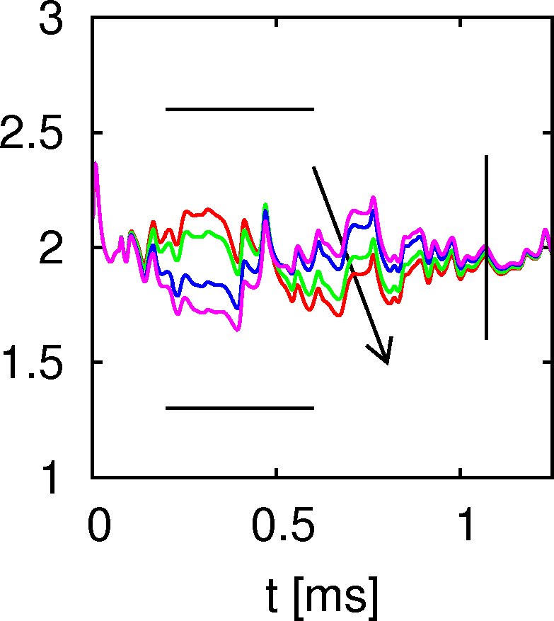
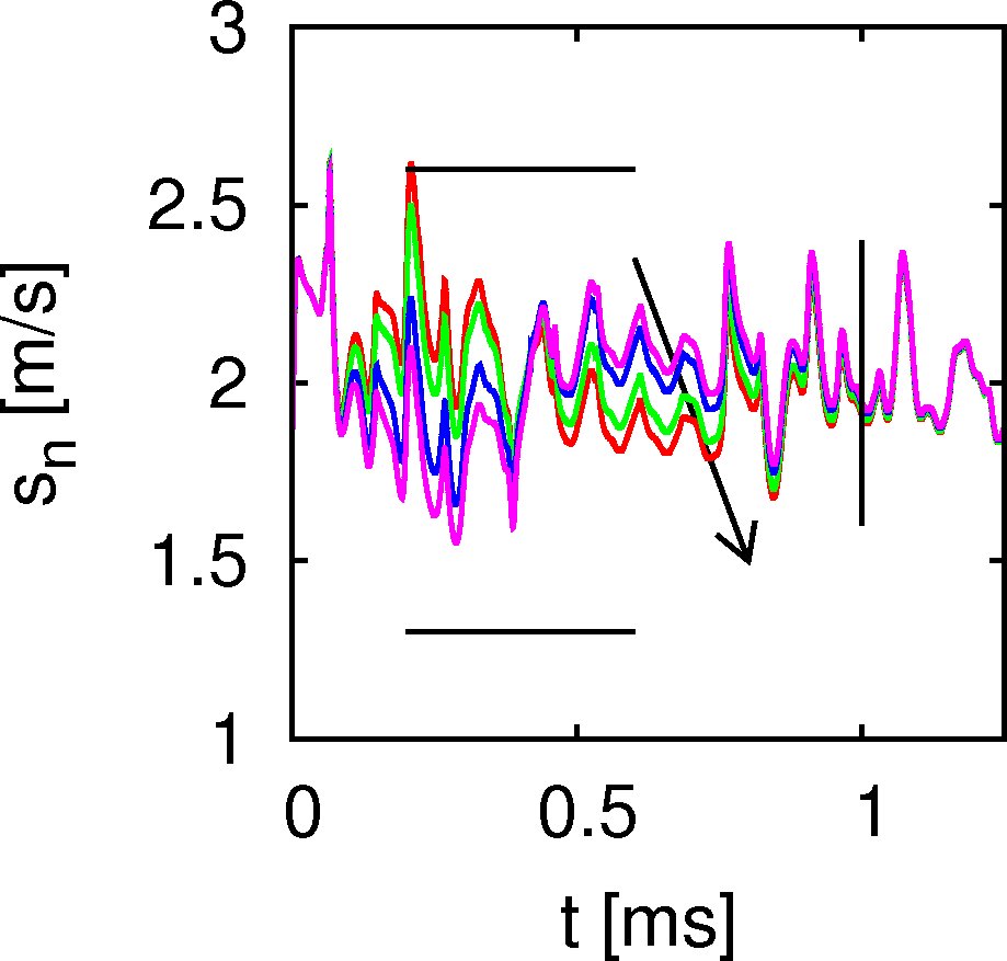
Figure 4: The burning velocity $s_{n}$ [m/s] against time $t$ [ms]: top left, Planar flame; top right, Cylindrical flame; bottom, Spherical flame. Four cases of equivalence ratio amplitude are shown in each figure, the thick arrow showing the direction of increasing amplitude: $A_{\phi}=0.2$ (red), $0.1$ (green), $-0.1$ (blue), $-0.2$ (purple). The theoretical bounds for stationary conditions at $\phi=1.2$ and $0.8$ are indicated by the horizontal lines. The vertical lines indicate the times when the curves come together as they leave the fuel oscillation cycle.

In the pressure spectra from the inwardly propagating flames, Figures 3(b) and 3(c), the lower frequencies $\omega<1000Hz$ are the forcing pressure frequencies (similar to Figure 3(a) from the planar flame). But at higher frequencies, $\omega>1000Hz$, the spectra in Figures 3(b) and 3(c) scale close to $\sim\omega^{-3}$ which is steeper than in the expanding expanding H2/air flames spectra, figure 3 in [Malik and Lindstedt (2010)], which scale close to $\sim\omega^{-2}$ over shorter ranges centred around $\omega\approx 5000Hz$. In the current simulations, the cylindrical flame spectrum in Figure 4(b) shows a steeper fall off from $\omega\approx 10,000Hz$, but the spherical flame spectra, Figure 4(c), continues to scale like $\sim\omega^{-3}$ even at very high frequencies.

The steeper spectral scaling indicates a weaker flame-pressure interaction than in the expanding flames although the excitations appear over a wider range of frequencies. Interestingly, the corresponding spectra from the expanding methane/air flames, figure 3 in [Malik and Lindstedt (2012)], also scale close to $\sim\omega^{-3}$.

As methane/air is a weakly reactive fuel compared to hydrogen/air, this indicates that negative curvature may be responsible for dampening flame-pressure interactions. Alternatively, as there is no strain ahead of the flame in contracting flames, then a reduction of strain-pressure interaction could also be responsible for the steeper fall off in the spectra. This is consistent with the expansing methane/air flame where the gas velocity is much smaller than in H2/air flames, resulting in low strain rates and overall weaker strain-pressure interactions.

4.2 Burning Velocity $s_{n}$

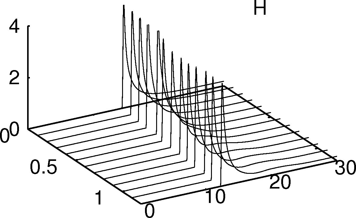
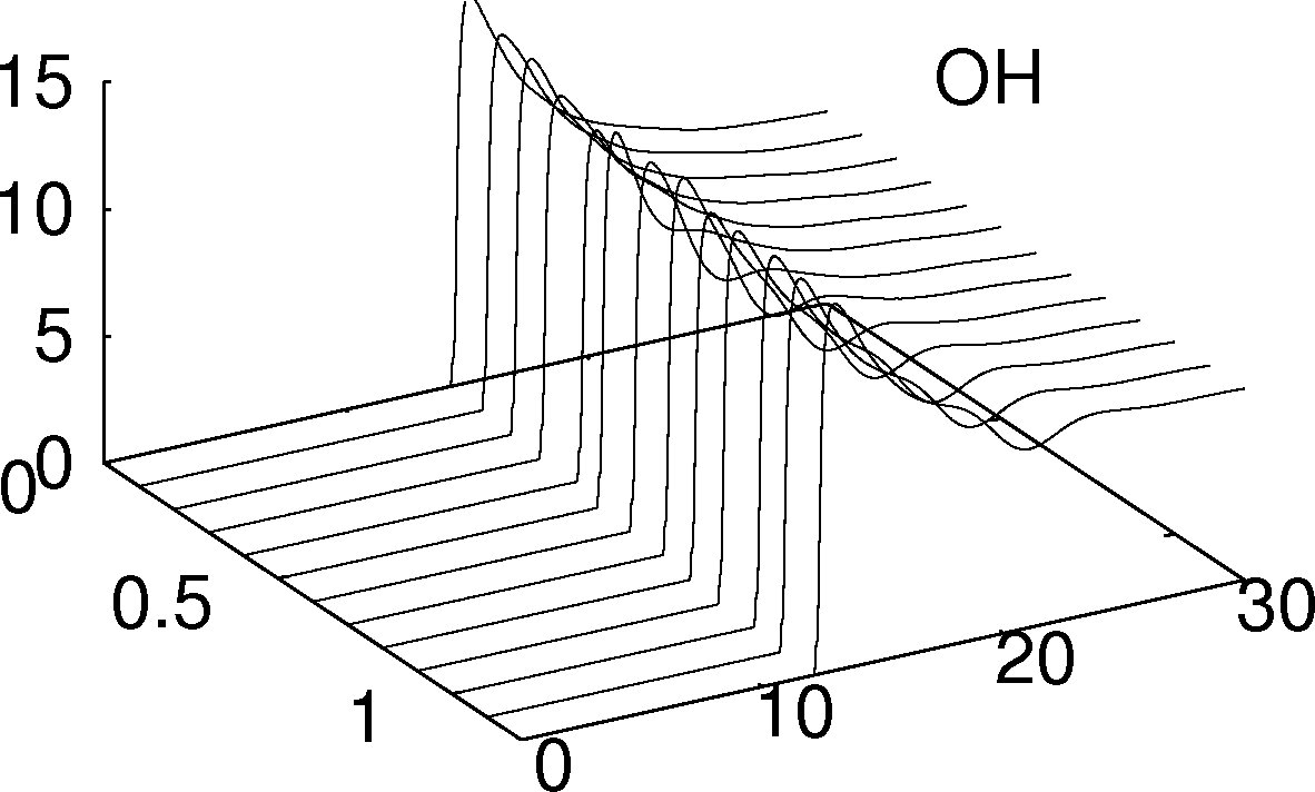
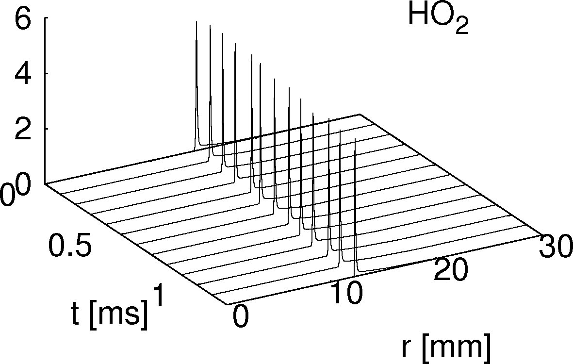
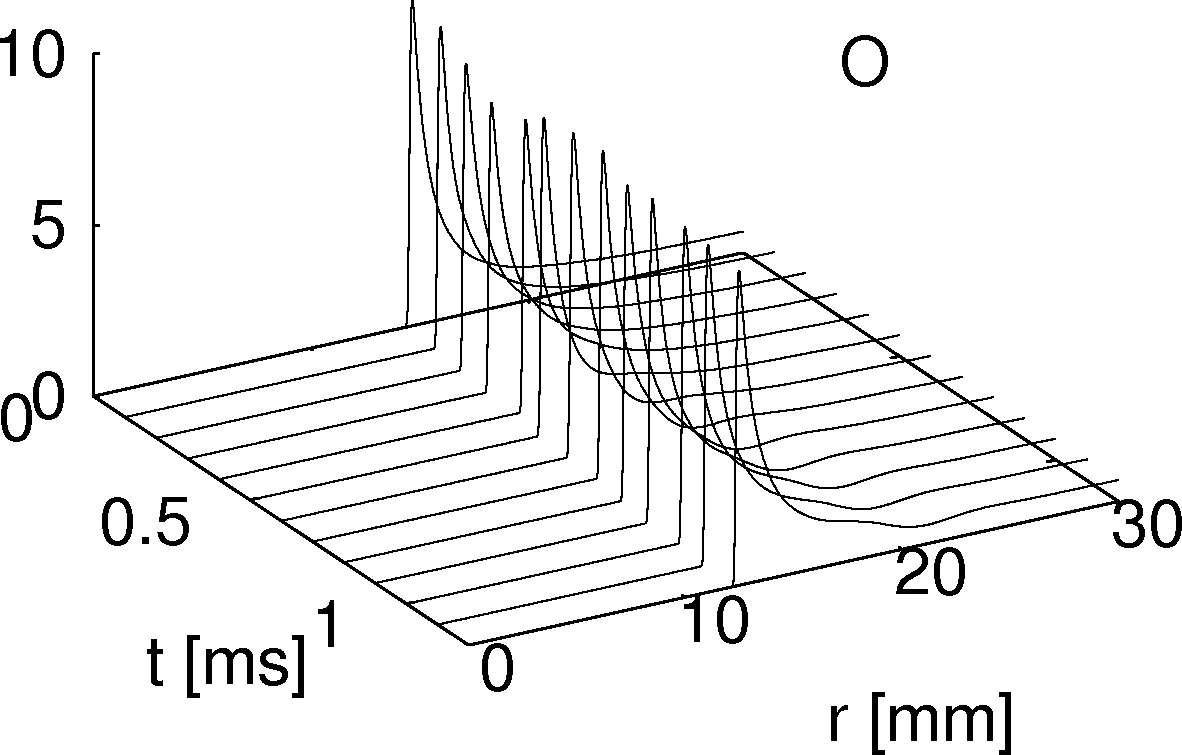
Figure 5: Mole–fractions of key chemical species, as indicated, at $0.05$ ms intervals, against time $t$ [ms] and radius $r$ [mm], from a cylindrical flame with $A_{\phi}=0.2$

We define the flame speed (burning velocity) as the rate of consumption of the fuel integrated across the flame,

$$s_{n} = {1\over\rho_{u}(Y_{F}^{u}-Y_{F}^{b})}\int_{-\infty}^{+\infty}\dot{R}_{F}M_{F}dr$$ (12)

where $F$ is the fuel ($H_{2}$), $M_{F}$ is the molecular weight of the fuel and $\rho_{u}$ is the density of the unburnt gases. $Y_{F}^{u}$ is the unburned fuel mass fraction and $Y_{F}^{b}$ is the burned fuel mass fraction (which is close to zero for stoichiometric and lean mixtures).

Figure 4 shows the flame speed $s_{n}[m/s]$ against time $t[s]$ as the flames propagate through the equivalence ratio oscillation cycle. The times when the flames leave the oscillation cycle are indicated by the vertical dashed lines.

Two trends are evident in Figure 4. First, the variation in the mean due to the underlying sinusoidal fuel distribution can be seen especially if one follows in time any one of the cases in the figures, say the red line corresponding to $A_{\phi}=0.2$. As this is an unsteady decaying system, molecular transport processes compete with the flame propagation from the start and partially smoothens out the fuel distribution as the flame moves through the fuel inhomogeneity. The effect is an approximately sinusoidal but decaying variation in the burning velocity $s_{n}$.

Second, superimposed on the mean trend are the higher frequency fluctuations in $s_{n}$ induced by the local flame-pressure interactions. As in the outwardly propagating hydrogen/air flames in [Malik and Lindstedt (2010)] periodic pressure fluctuations reflecting back from the open boundary and impacting on the reaction layer is evident especially in the spherical flame where the focusing of pressure waves towards the centre is the strongest.

The flame speed $s_{n}$ does not approach the limits corresponding to the upper and lower bounds of the initial fuel distributions at $\phi=1.2$ and $\phi=0.8$ respectively, indicated by the two horizontal lines in Figure 4. This is partially due to the smoothening out of inhomogeneities due to action of molecular transport processes; this is an unsteady system and by the time that the flame arrives at the point where $\phi$ was initially at its peak value of $1.2$, the local value of $\phi$ is now closer to the mean value of $1$, i.e. $1<\phi<1.2$. Similar considerations apply to the lower bound where now $0.8<\phi<1$. (However, we would expect the upper and lower bounds to be approached if the fuel distribution were stationary which would be possible if the molecular diffusion were very small.)

It is also possible that the flame response to the local rate of heat release is affected by a memory effect which could also prevent the flame speed from attaining to its extreme values. Memory effects are discussed further in section 4.5.

4.3 Relaxation number $n_{R}$

The relaxation time $\tau_{R}$ is the time it takes the flame speed to return to the mean value once disturbed. From Figure 4 $\tau_{R}$ is the time after which the different $s_{n}$-curves come to within 5% of the mean value $\phi=1$ and remain together thereafter. These times are indicated by the vertical lines in Figure 4.

A non-dimensional relaxation number $n_{R}$ is defined, [Malik and Lindstedt (2012)], as

$$n_{R} = {\tau_{R}\over\tau_{L}}$$ (13)

which is the ratio of the relaxation time to a flame time scale $\tau_{L}$. $n_{R}$ is a function of stretch, molecular transport processes, the fuel distribution, and possibly also of the pressure fluctuations. In general, we expect $n_{R}$ to be a function of many parameters including Schmidt number, Prandtl number and Lewis numbers. For example for small Schmidt numbers, the smoothening of the fuel distribution inhomogeneities due to the stronger molecular diffusion could be more rapid leading to smaller relaxation numbers.

In [Malik and Lindstedt (2010)] it was noted how effectively positive stretch reduces the relaxation times $\tau_{R}$ by about 40%: from $\sim 1.1$ ms (planar), to $\sim 0.8$ ms (cylindrical); and $\sim 0.65$ ms (spherical). In contrast, from Figure 4 negative curvature reduces $\tau_{R}$ by only about 10% from the stretch-free planar flame case: we have $\tau_{R}\sim 1.07ms$ in the inwardly propagating cylindrical flame, and $\sim 1.0ms$ in the spherical flame case.

However, the non-dimensional $n_{R}$ from both the expanding H2/air and expanding CH4/air flames were found to be similar and to follow the same trend: $n_{R}$ reduces by about 30% going from planar to spherically CH4/air flames and about 40% in the H2/air flames. Table 2 shows the relaxation times $\tau_{R}$ and the relaxation numbers $n_{R}$ from the present imploding H2/air flames, and also from the two expanding flames (from [Malik and Lindstedt (2012)]) for comparison.

In defining $n_{R}$ from equation (4.2), we have used $\tau_{L}\sim\delta_{L}/s_{L}$ and the flame thickness $\delta_{L}$ is taken as the width of the fuel reaction rate profile $\dot{R}_{F}$, as discussed in [Malik and Lindstedt (2012)]. From the current implosion simulations we obtain $n_{R}\approx 4.5$ in the cylindrical flame, and $n_{R}\approx 4.2$ in the spherical flame.

	$\Large\tau_{R}$ [ms]			$\Large n_{R}$
Propagation Mode	Planar	Cylindrical	Spherical	Planar	Cylindrical	Spherical	Reference
H2/air imploding	$1.1$	$1.07$	$1.00$	$4.6$	$4.5$	$4.2$	Current
H2/air expanding	$1.1$	$0.80$	$0.65$	$4.6$	$3.3$	$2.7$	a
CH4/air expanding	$6.0$	$4.50$	$4.00$	$4.4$	$3.3$	$3.0$	b

Table 2. Relaxation times $\tau_{R}$ and the relaxation numbers $n_{R}$ for hydrogen–air and methane–air flames. References: a – [Malik and Lindstedt (2010)]; b – [Malik and Lindstedt (2012)]

The results shown in Table 2 are consistent with the spectral results observed in section 4.1 where negative stretch in imploding flames appears to interact more weakly with the pressure fluctuations than with positive stretch in expanding flames. The weaker interaction manifests itself here as a smaller reduction in the relaxation number $n_{R}$.

4.4 Unsteady thermochemical flame structure

The response of the thermochemical flame structure to the unsteady processes is shown in Figure 5 where the mole-fraction profiles of selected species against time and radius at 0.1ms intervals are shown from the cylindrical flame (spherical flames produce qualitatively similar results).

Figures 6 and 7 show the mole-fraction profiles against the radius of all the species (except inert nitrogen) in, respectively, the cylindrical and spherical flames at 0.125ms intervals.

The stable species, such as $H_{2}$ and $H_{2}O$, show little response to the oscillations most probably because they are already ‘saturated’ at high concentration levels and so small oscillations in the mole-fractions produces little effect.

The observed response of the thermochemical structure in these figures is similar to that found in the positively stretched flames in [Malik and Lindstedt (2010), Malik and Lindstedt (2012)]. A spectrum of chemical species thickness $\{l_{k}\}$ rather than a single global flame thickness $\delta_{L}$ seems more appropriate in characterising flame structure.

We may reasonably extend this idea to fluctuations in any physical variable that alters the flame structure, and suggest the existence of an associated spectrum of non-dimensionalised length scales $\{S_{k}\}$,

$$S_{k} = {l_{k}\over\lambda}\qquad k=1,2,...,N$$ (14)

where $\lambda$ is a characteristic length scale of the physical fluctuations. Thin profiles of those species such that $S_{k}\ll 1$ will not be significantly affected except in amplitude — such as $HO_{2}$ and $H_{2}O_{2}$; but the thicker profiles of those species with $S_{k}\gg 1$ will also be perturbed across their whole length because such oscillations can penetrate inside their structure – such as $OH$; while stable species, such as $H_{2}$, $O_{2}$ and $H_{2}O$ are likely to be unaffected for the reason noted above. Other species display intermediate stages of profile disturbance depending on the thickness of their profile.

  

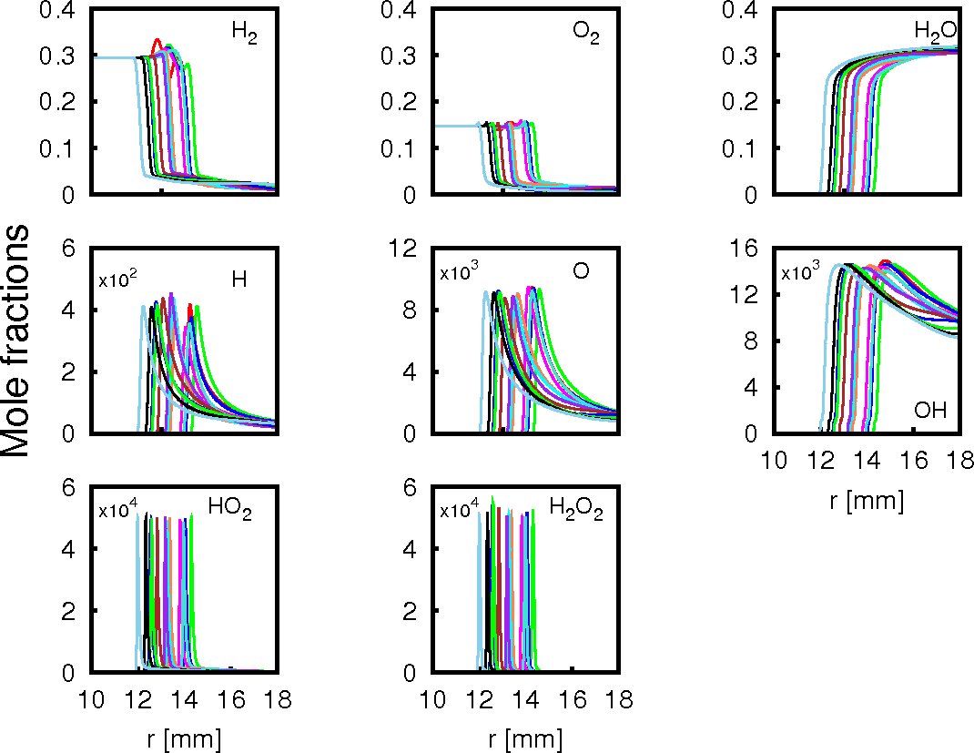
Figure 6: Mole–fractions $X_{k},\quad k=1,2,...,8$ of all chemical species (except Nitrogen), as indicated on each plot, at $0.1$ ms intervals against the radius $r[mm]$, from the cylindrical flame with $A_{\phi}=0.2$. The mean flame propagation is from right to left (the centre).

  

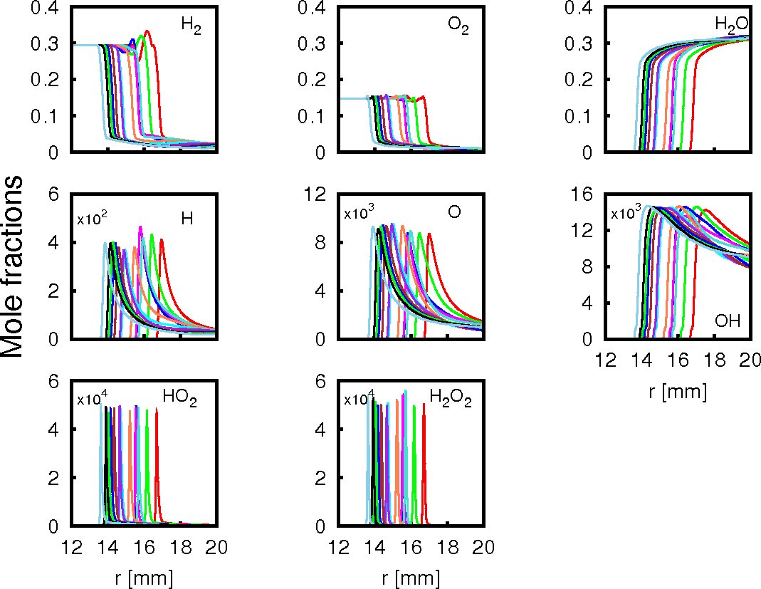
Figure 7: As Figure 6, but for the spherical flame

4.5 Time-lag and ‘flapping’

An issue of practical and theoretical interest is the impact of the physical oscillations on the chemical balance and heat release inside the disturbed flame kernel and the consequent induced time–lag.

Figure 8 shows the profiles at 0.1ms intervals, from the cylindrical flame simulations with $A_{\phi}=0.2$, of (a) the rate of heat release $\dot{h}$, (b) the mole-fractions of H-radical, and (c) the mole-fractions of O-radical. Figure 9 shows similar profiles from the spherical flames.

     

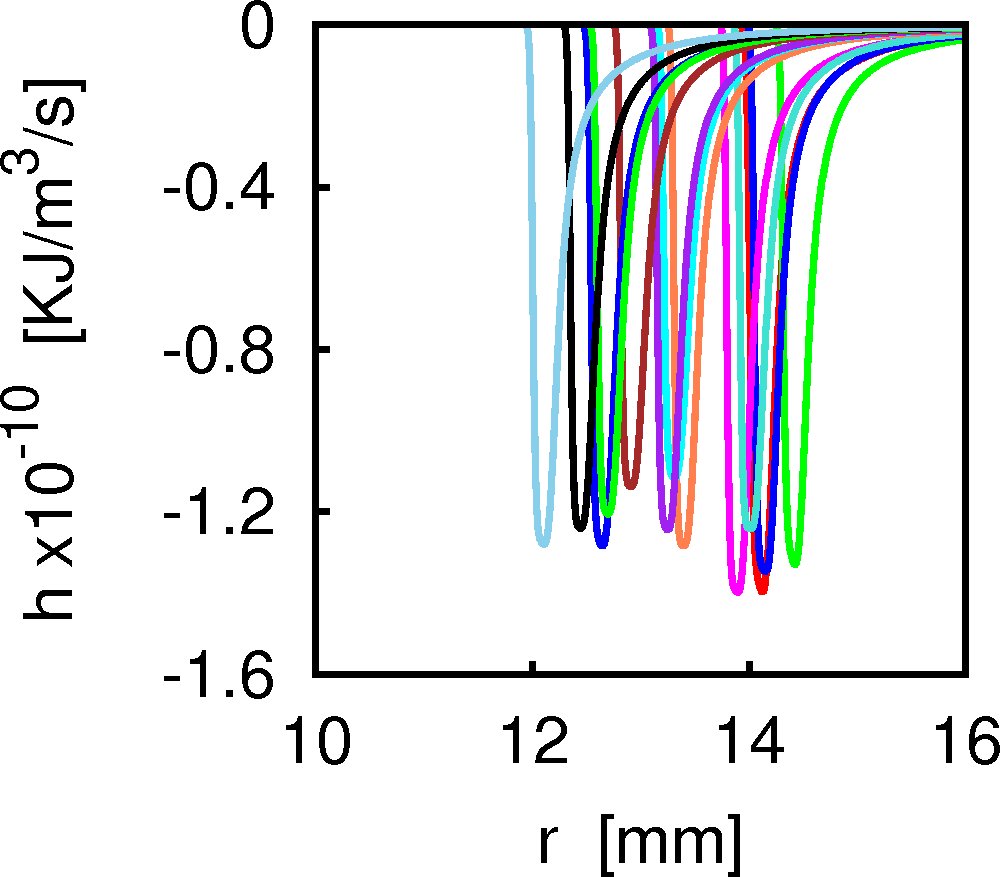
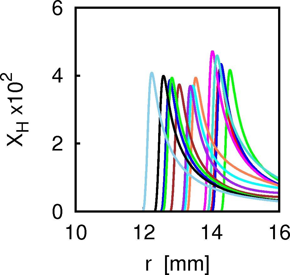
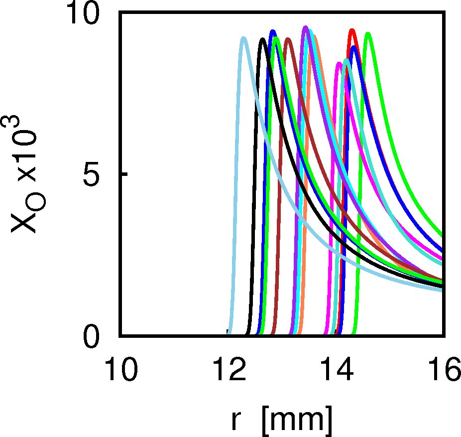
Figure 8: Top: Rate of heat release per unit volume $\dot{h}$ $[KJ/m^{3}/s]$ against the radius $r$ [mm] at 0.1ms intervals, from the cylindrical flame with $A_{\phi}=0.2$. Corresponding mole-fractions of, Bottom left: H-radicals, Bottom left: O-radicals. The mean flame propagation is from right to left (the centre).

     

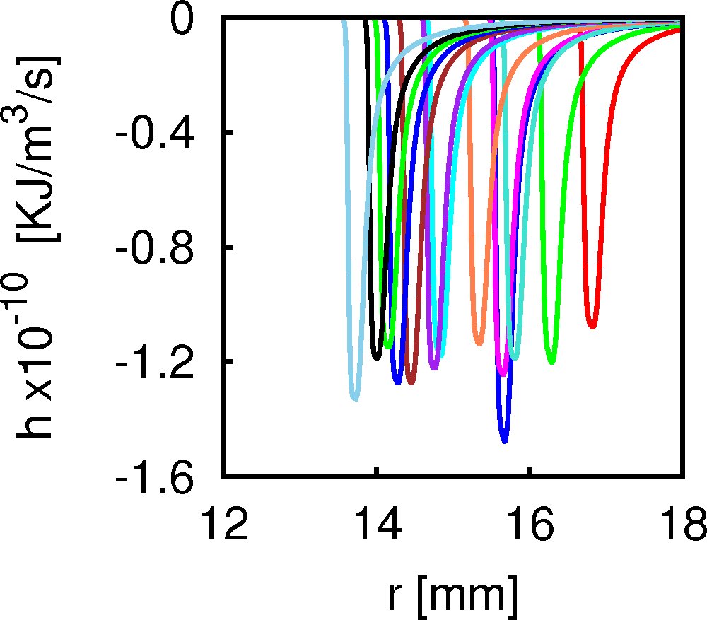
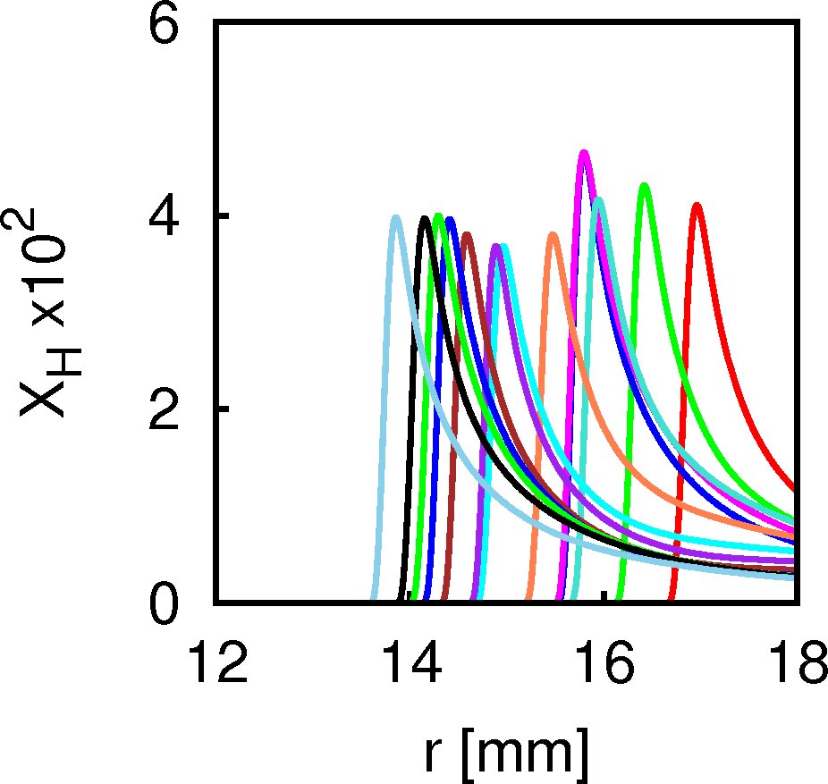
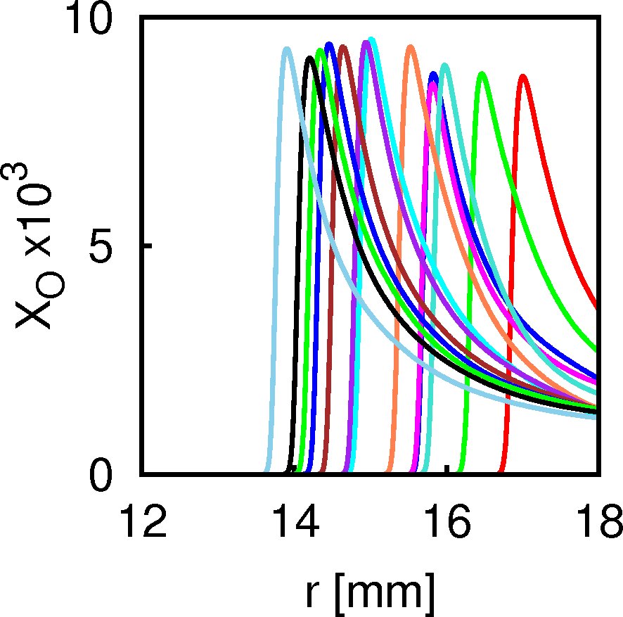
Figure 9: As Figure 8, but for a spherical flame.

In [Malik and Lindstedt (2010), Malik and Lindstedt (2012)], some evidence of time–lag between the rate of heat release and the species response was observed in the flames with zero and positive stretch. A correlated response is more difficult to observe in the flames with negative curvature in figures 8 and 9 because the flames are convected back and forth rapidly –smoothen ‘flapping’ – by the pressure induced velocity fluctuations $u_{p}^{\prime}$ (section 4.2). The general expression for the flame front velocity is

$$u_{f} = s_{n}+u_{g}+u^{\prime}_{p},$$ (15)

where $u_{g}$ is the gas velocity, and $\langle u_{p}^{\prime}\rangle=0$, where the angled brackets represents the ensemble average.

Flapping of the flame front by pressure induced fluctuations is always present, but it has rarely been observed because in expanding flames, the most commonly studied case, the gas velocity is much bigger than the fluctuating component, $|u_{g}|\gg|u^{\prime}|$. But in the current contracting flames where $u_{g}=0$ and we have $u_{f}=s_{n}+u^{\prime}_{p}$, and the rms $u^{\prime}_{p}$ is comparable to the burning velocity, $|u^{\prime}_{p}|_{\rm rms}\approx|s_{n}|$, and therefore the flapping of the flame front is much more apparent causing the flame fronts at different times to appear scrambled.

Nevertheless, an average trend is observable in Figures 8 and 9, with the $H$ and $O$ radical concentrations approximately anti-correlated (most likely due to the main chain branching reaction $H+O_{2}=O+OH$), and the peaks in the respective profiles correlating quite well indicating a short time–lag.

The results from the previous sections have indicated that inwardly propagating flames interact weakly with pressure oscillations, and therefore we can expect that these flames will behave more like planar flames, and therefore the chemical balance inside the flame kernel will remain well correlated to the rate of heat release with short time-lags. The average trend noted above provides some support for this.

5 Discussion

In this study the transient response of premixed negatively stretched hydrogen/air flames at mean atmospheric pressure and at mean stoichiometry, subjected simultaneously to equivalence ratio variations and to naturally decaying pressure fluctuations at frequencies and length scales that can couple to the flame structure has been explored numerically using an implicit method well suited to resolve stiff and unsteady chemically reacting systems.

A comparison with the positively stretched H2/air [Malik and Lindstedt (2010)] and CH4/air flames [Malik and Lindstedt (2012)] was carried out, and a number of important features have emerged. Pressure oscillations in the range $200-1000$Hz produce steeper spectral broadening which scale close to $E_{p}\sim\omega^{-3}$, as compared to the corresponding positively stretched H2/air flame spectra which scaled close to $E_{p}\sim\omega^{-2}$. This indicates a weaker flame-pressure response in negatively stretched flames, although the spectral broadening occurs across a wider range of frequencies; in the case of imploding spherical flames the range of excited frequencies extends to very high frequencies. It is interesting that the expanding CH4/air flames also produced spectra close to $E_{p}\sim\omega^{-3}$.

The non-dimensional relaxation number $n_{R}$ is defined as the ratio of the relaxation time to a flame time scale $n_{R}={\tau_{R}/\tau_{L}}$; it is a function of stretch, molecular transport processes, fuel distribution, and the frequency and amplitude of the fluctuations. $n_{R}$ contains information about the competing processes of flame propagation and molecular transport: if molecular diffusion is dominant then we would expect $n_{R}$ to be small. $n_{R}$ may also be indicative of flame stability to external disturbance in the sense that a smaller values of $n_{R}$ means that the reactive-diffusive system returns to mean conditions quickly indicating greater flame stability.

The relaxation number $n_{R}$ was found to decrease by only 10% with increasing negative stretch (flow divergence) in H2/air flames compared to the zero stretch planar flame case; but $n_{R}$ was found to decrease by about 40% with increasing positive stretch in H2/air flames in [Malik and Lindstedt (2010)]. Negative stretch thus appears to couple less strongly with dynamic processes such as pressure fluctuations and transport processes than does positive stretch, because it reduces the relaxation number to a lesser extent than the latter. This picture is consistent with the spectral analysis mentioned above.

This point is further strengthened by the fact that the trends in $n_{R}$ in both the H2/air and CH4/air expanding flames is similar, see Table 2, even though H2/air and CH4/air are at opposite ends of the ’reactivity’ scale, H2/air being a very reactive mixture. $n_{R}$ thus appears to more strongly correlated with the sign of the curvature than with the thermo-chemistry of different flame types. This may in part be due to the fact that both curvature and strain contribute to positive stretch in expanding flames, but curvature alone contributes to negative stretch in imploding flames because of the absence of strain (gas velocity) ahead of the flame, $u_{g}=0$.

$n_{R}$ is potentially important as a non-dimensional time for an inhomogeneous system to return to the mean conditions when subjected to external perturbations. It may have significance for automotive engines where such conditions are prevalent; if a system has a short relaxation time then it attains to mean conditions rapidly and therefore mean field modeling strategies could be effective.

For moderate levels of inhomogeneity $A_{\phi}\ll 1$, and short length scales $\lambda=1mm$ and pressure fluctuations in the frequency range $\omega\sim 200-1000Hz$, the molecular transport processes are competitive with flame propagation and partially reduce the fuel inhomogeneities during the time that the flame moves through the fuel oscillation cycle, such that the upper and lower limits of the flame speed $s_{n}$ are not attained. Negative curvature appears not to alter this process significantly under the conditions of the simulation, which again is consistent with the spectral and the relaxation number analysis, which both indicate reduced strengths of flame-pressure coupling with negative curvature.

Flapping of the flame induced by the pressure fluctuations is much more prominent in inwardly propagating flames due to the zero gas velocity ahead of the flame $u_{g}=0$. This is seen in the scrambling of the flame fronts in successive short time frames seen in Figures 8 and 9. Flapping has rarely been observed before because the large gas velocity in expanding flames, the most commonly observed case, overwhelms the flapping since $|u_{g}|\gg|u^{\prime}|$.

Flapping may have consequences for other effects such as spectra, relaxation numbers and time-lag through non-linear coupling of the flame-front with the chemical kinetics and molecular transport processes. But in view of the weaker flame-pressure coupling observed in negatively stretched flames it is reasonable to assume that the effect on time-lag will also be weaker so that the chemical balance in the flame kernel will remain close to the zero stretch (planar flame) case. The flame structure will then be well correlated with the rate of heat release and this will lead to a short time-lag as the flame attempts to adjust to the unsteady local conditions. Such a trend in the mean is observed over short times in Figures 8 and 9.

However, it is possible that different conditions – such as stronger pressure fluctuations, stronger inhomogeneity, stronger stretch, different fuels, and lean/rich conditions – could produce stronger or weaker disruption to the chemical balance through coupling with non-linear transport processes and pressure fluctuations. To some extent this has already been observed in outwardly propagating mode in [Malik and Lindstedt (2010), Malik and Lindstedt (2012)] where the impact of positive stretch was stronger. [Johannessen et al (2011)] have looked at turbulent premixed hydrogen flames and observed dominant kinetics or dominant pressure effects, depending upon fuel-lean and fuel-rich conditions. However, it is not yet known whether this is specific to hydrogen flames.

The response of the thermochemical structure to pressure and fuel distribution fluctuations is similar to that observed in the expanding flames in [Malik and Lindstedt (2010), Malik and Lindstedt (2012)]. The evidence suggests that we can characterise flame response by a spectrum of non-dimensional length scales $\{S_{k}=l_{k}/\lambda\}\quad k=1,2,...,N$, where $l_{k}$ is the lengths scale of the $k^{\prime}th$ species, and $\lambda$ is the scale of the physical oscillations (pressure oscillations in the current study). We find that all species oscillate in their peak concentrations in response to the local pressure and fuel distribution; but thick unstable species with $S_{k}\gg 1$ are also disturbed across their entire length. The major stable species concentrations are ‘saturated’ at high levels and the induced fluctuations are too small to be observable in their profiles.

The study reported here is of importance to combustion processes at a fundamental level as well as to practical devices such as automotive engines and gas turbines. Engines for example increasingly use lean fuel mixtures and there is also a trend towards the use of alternative fuels, such as biofuels. This requires the study of lean combustion processes for the prediction of emissions levels, which in turn requires the inclusion of realistic chemistry coupled to the compressible flow. The method used here demonstrates that detailed numerical studies of such complexity is now possible.

6 Conclusions

The implicit method TARDIS, [Malik and Lindstedt (2010), Malik and Lindstedt (2012), Malik (2012)], has provided a platform to explore finite thickness premixed flames in great detail because of its capability of coupling the fully compressible flow to the comprehensive (realistic) chemistry and detailed transport properties. The implicit nature of the solver gives it stability, and it resolves all the temporal and spatial scales in the systems examined here. This feature allows very complex systems in unsteady contexts to be explored, and as such is a step towards more realistic combustion simulations.

We have explored negatively stretched hydrogen/air flames subjected to fluctuations in pressure and fuel distributions. The impact of increasing negative stretch was investigated through the use of planar, cylindrical and spherical geometries, and a comparison with the results from expanding hydrogen/air flames in [Malik and Lindstedt (2010), Malik and Lindstedt (2012)] was made. Imploding flames are of interest because they have rarely been studied and also because only negative curvature contributes to the stretch so that the effects of curvature can be studied in isolation.

Overall, we have found that the results from axi-symmetric (cylindrical) flames are qualitaively similar to those from the corresponding spherical flames. This is consistent with the previous studies for expanding H2/air flames, [Malik and Lindstedt (2010)], and expanding methane/air flames, [Malik (2012)]. This suggests that it is the fuel type and the flame propagation mode that are the dominant features in the these systems.

The flame relaxation number $n_{R}=\tau_{R}/\tau_{L}$, (where $\tau_{R}$ is the time that the flame speed $s_{n}$ takes to return to the mean equilibrium conditions after initial disturbance; $\tau_{L}$ is a flame time scale) contains information about competing processes of flame propagation and molecular transport. $n_{R}$ decreases by only 10% with increasing negative stretch, and by about 40% in expanding flames with positive stretch in [Malik and Lindstedt (2010), Malik and Lindstedt (2012)], see Table 2.

Furthermore, the fluctuating pressure spectra $E_{p}(\omega)$ scale close to $\sim\omega^{-3}$, which is steeper than in the expanding H2/air flames which scales like $\sim\omega^{-2}$, but is close to the spectra observed in the expanding CH4/air flames.

The flame relaxation number $n_{R}$ appears to be far more sensitive to variations in positive and negative curvature than it is to the different thermo-chemistry in different flame types. The decrease in $n_{R}$ is much less with negative curvature than with positive curvature. $n_{R}$ may therefore be an indicator of flame-curvature coupling, and the results here may indicate that negative curvature couples less strongly to the flame thermo-chemistry than in positive curvature flames, which is consistent with the spectral analysis mentioned above. However this needs more investigation and is the subject of current ongoing work.

Rapid flapping of the flame front by the random velocity fluctuations induced by the pressure fluctuation is prominent again due to the lack of gas velocity ahead of the flame. ‘Memory effects’ between fuel consumption and the rate of heat release is obscured by the flapping, although on theoretical grounds we expect inwardly propagating flames to have shorter time-lags than in positively stretched flames.

A spectrum of species thickness $\{S_{k},k=1,2..,N\}$ exists such that species formed in thin reaction layers are generally not disturbed except in their peak concentrations. Stable species profiles are unaffected by small levels of oscillations. Thus, it may be more useful to characterise the internal structure of flames in terms of a spectrum of length scales rather than in terms of a single flame thickness.

Acknowledgment

The authors wish to thank SABIC for funding this work through grant number SB101018, and also the Information Technology Center at King Fahd University of Petroleum and Minerals for providing High Performance Computing resources that have contributed to the results reported in this paper.

References

- Baillot et al (2002). Baillot, F., Durox, D. and Demare, D. 2002 Experiments on imploding spherical flames: effects of curvature. Proc. Combust. Inst., 29, 1453–1460.
- Bradley et al (1996). Bradley, D., Gaskell P., and Gu, X.J. 1996 Burning velocities, markstein lengths and flame quenching in spherical ethane–air flames: A computational study. Combust. Flame, 104, 176–198.
- Candel (2002). Candel S. 2002 Combustion dynamics and control: Progress and challenges. Proc. Combust. Inst., 29, 1–28.
- Chakraborty and Cant (2004). Chakraborty N. and Cant R.S. 2004 Unsteady effects of strain rate and curvature on turbulent premixed flames in an inflow-outflow configuration. Combust. Flame, 137,129–147.
- Chen et al (2006). Chen, J.H., Hawkes, E.R., Sankaran, R., Mason, S D. and Im, H. G. 2006 Direct numerical simulation of ignition front propagation in a constant volume with temperature inhomogeneities: I. Fundamental analysis and diagnostics. Combustion and Flame, 145(1–2), 128–144.
- Christiansen and Law (2002). Christiansen E.W. and Law C.K. 2002 Pulsating Instability and extinction of stretched premixhyrdrogened flames Proc. Combust. Inst., 29, 61–68.
- Clavin and Williams. Clavin P. P. and Williams F.A. 1982 J. Fluid Mech., 116, 251.
- Clavin 1985. Clavin P. 1985 Prog, Ener. Combust. Sci., 11:1.
- Dowdy (1990). Dowdy, D.R., Smith, D.B. and Taylor, S.C. 1990 The use of expanding spherical flames to determine burning velocities and stretch effects in hydrogen/air flames. Proc. Combust. Inst, 23, 325–332.
- Dyer and Korakianitis (2007). Dyer, R. S. and Korakianitis T. 2007 Pre-integrated response map for inviscid propane-air detonation. Combustion Science and Technology, 179(7), 1327–1347.
- Gou et al (2010). Gou, X., Sun, W., Chen, Z., and Ju, Y. 2010 A dynamic multi-timescale method for combustion modeling with detailed and reduced chemical kinetic mechanisms. Combustion and Flame, 157(6), 1111–21.
- Groot and De Goey (2002). Groot, G.R.A. and De Goey, L.P.H. 2002 A computational study on propagating spherical and cylindrical premixed flames. Proc. Combust. Inst., 29, 1445–1451.
- Gummalla and Vlachos (2000). Gummalla, M. and Vlachos, D.G. 2000 Complex dynamics of combustion flows by direct numerical simulations Phys. Fluids, 12, 2520–255.
- Hamakhan and Korakianitis (2010). Hamakhan, I.A. and Korakianitis, T. 2010 Aerodynamic performance effects of leading edge geometry in gas turbine blades. Applied Energy, 87(5), 1591–1601.
- Heywood (1988). Heywood, J. B. 1988 Iternal Combustion Engine Fundamentals. McGraw-Hill.
- Ibrahim et al (2009). Ibrahim, S.S., Gubba, S.R., Masri, A.R. and Malalasekera, W. 2009 Calculations of explosion deflagrating flames using a dynamic flame surface density model. J. Loss Prevention in the Process Industries, 22(3), 258–264.
- Jiang et al (2007). Jiang, X., Zhao, H. and K.H. Luo. 2007 Direct numerical simulation of a non-premixed impinging jet flame. ASME J. Heat Transfer, 129(8), 951–957.
- Johannessen et al (2011). Johannessen, B., Løvås, T. and Gruber, A. 2011 Modeling turbulent reactive flows for engineering applications Proc. of MekIT2011, 5-22.
- Karpov et al (1997)). Karpov, V.P., Lipatnikov, A.N. and Wolanski, P. 1997 Finding the markstein number using the measurement of expanding spherical flames. Combust. Flame, 109, 436–448.
- Kelley and Law (2009). Kelley, A.P. Kelley and Law, C.K. (2009). Nonlinear effects in the extraction of Laminar flame speeds from expanding spherical flames. Combustion and Flame 156(9), 1844–51.
- Korakianitis (1993). Korakianitis, T. 1993 Prescribed-curvature distribution airfoils for the preliminary geometric design of axial turbomachinery cascades. Transactions of the ASME, Journal of Turbomachinery, 115(2), 325–333.
- Korakianitis and Papagiannidis (1993). Korakianitis, T. and Papagiannidis, P. 1993 Surface-curvature-distribution effects on turbine-cascade performance. Transactions of the ASME, Journal of Turbomachinery, 115(2), 334–341.
- Korakianitis et al (2004). Korakianitis, T. Dyer, R. S. and Subramanian, N. 2004 Pre-integrated non-equilibrium combustion-response mapping for gas-turbine emissions. Transactions of the ASME, Journal of Engineering for Gas Turbines and Power, 126(2), 300–305.
- Korakianitis et al (2007). Pachidis, V., Pilidis, P., Templexakis, I., Korakianitis, T. and Kotsiopoulos, P. 2007 Prediction of engine performance under compressor inlet flow distortion using streamline curvature. Transactions of the ASME, Journal of Engineering for Gas Turbines and Power, 129(1), 97–103.
- Kown et al (1992). Kwon S., Tseng L.K., & Faeth M. 1992 Laminar burning velocities and transition to unstable flames in and mixtures. Combust. Flame, 90, 230–246.
- Lai et al (2007). Lai, H., Zhou, S.P. and Luo, K.H. 2007 Large eddy simulation and computational aeroacoustics of an unsteady three-dimensional compressible cavity flow. J. Eng. Thermophys., 28(5), 1–4.
- Lauvergne and Egolfopoulos (2000)). Lauvergne, R. and Egolfopoulos, F.N 2000 Unsteady response of C3H8=air laminar premixed flames submitted to mixture composition oscillations. Proc. Combust. Inst., 28, 1841–1850.
- Lieuwen (2005). Lieuwen, T. 2005 Nonlinear kinematic response of premixed flames to harmonic velocity disturbances. Proc. Combust. Inst., 30, 1725–1732.
- Lignell et al (2008). Lignell, D.O., Chen, J.H. and Smith, P.J. 2008 Three-dimensional direct numerical simulation of soot formation and transport in a temporally evolving nonpremixed ethylene jet flame. Combust. Flame, 155, 316–333.
- Lindstedt et al (1998). Lindstedt, R.P., Meyer, M.P. and Sakthitharan, V. 1998 Direct simulation of transient spherical laminar flame structures. Eurotherm Seminar 61 on Detailed Studies of Combustion Phenomena, 1(D), 53–74.
- Lipatnikov (1996)). Lipatnikov, A.N. 1996 Some issues of using markstein number for modeling premixed turbulent combustion. Combust. Sci. Tech., 119, 131–154.
- Løvås et al (2010). Løvås, T., Malik, N.A. and Mauss, F. 2010 Global reaction mechanism for ethylene flames with preferential diffusion. Comb. Sci. Tech., 182, 1945–60.
- Lu and Law (2009). Lu, T. and Law, C.K. 2009 Toward accommodating realistic fuel chemistry in large-scale computations. Prog. Ener. Combus. Sci., 25, 192–215.
- Luff (2006). Luff, D.S. 2006 Experiments and Calculations of Opposed and Ducted Flows. Doctoral dissertation, Imperial College London.
- Malalasekera et al (2008). Malalasekera, W., Ranga-Dinesh, K.K., Ibrahim, S.S. and Masri, A.R. 2008 LES of recirculation and vortex breakdown of swirling flames. Combust. Sci. Tech., 180(5), 809–832.
- Malik (2012). Malik, N.A. 2012 Non-linear power laws in stretched flame velocities in finite thickness flames: a numerical study using realistic chemistry. To appear in Combust. Sci. Tech 2012.
- Malik and Lindstedt (2010). Malik, N.A. and Lindstedt, R.P. 2010 The response of transient inhomogeneous flames to pressure fluctuations and stretch: planar and outwardly propagating hydrogen/air lames. Combust. Sci. Tech., 182(9), 1–22.
- Malik and Lindstedt (2012). Malik, N.A. and Lindstedt, R.P. 2012 The response of transient inhomogeneous flames to pressure fluctuations and stretch: planar and outwardly propagating methane/air flames To appear in Combust. Sci. Tech. 2012.
- Marchal et al (2009). C. Marchal, J-L. Delfau, C. Vovelle, G. Moréac, C. Mounam-Rousselle, and F. Mauss. 2009 Modeling of aromatics and soot formation from large fuel molecules. Proc. Combust. Inst., 32(1), 753–759.
- Markstein (1964). Markstein, G.H. 1964 Non-steady Flame Propagation. Pergamon Press.
- Marzouk et al (2000). Marzouk, Y.M., Ghoniem, A.F. and Najm, H.N. 2000 Dynamic response of strained premixed flames to equivalence ratio gradients. Proc. Combust. Inst., 28, 1859–1866.
- Mason and Monchick (1962). Mason, E.A. and Monchick, L. 1962 Heat conductivity of polyatomic and polar gases. J. Chem Phys., 36, 1622–1639.
- Meyer (2001). Meyer, M.P. 2001 The Computation of Steady and Transient Laminar Flames. PhD Thesis, Imperial College London.
- Mauss et al (2006). Mauss, F., Netzell, K. and Lethtiniemi, H. 2006 Aspects of modeling soot formation in turbulent diffusion flames. Comb. Sci. Tech., 178, 1871–1885.
- Najm and Wyckoff (1997). Najm, H.N. and Wyckoff, P.S. 1997 Premixed flame response to unsteady strain rate and curvature. Combust. Flame, 110, 92–112.
- Noskov et al (2007). Noskov, M, Benzi, M. and Smooke, M.D. 2007 An implicit compact scheme solver for two-dimensional multicomponent flows. Computers and Fluids, 36(2), 376–397.
- Noskov and Smooke (2005). Noskov, M. and Smooke, M. D. 2005 An implicit compact scheme solver with application to chemically reacting flows. J. Comp. Physics, 293(2), 700–730.
- Pachidis et al (2006). Pachidis, V., Pilidis, P., Talhouarn, F., Kalfas, A., and I. Templalexis. 2006 A fully integrated approach to component zooming using computational fluid dynamics. Transactions of the ASME, Journal of Engineering for Gas Turbines and Power, 128(3), 579–584.
- Reid and Sherwood (1960)). Reid, R.C. and Sherwood, T.K. 1960 Properties of gases and Liquids: their estimation and correlation. McGraw-Hill.
- Sankaran and Im (2002). Sankaran, R. and Im, H.G. 2002 Dynamic flammability limits of methane/air premixed flames with mixture composition fluctuations. Proc. Combust. Inst., 29, 77–84.
- Schroll et al (2009). Schroll, P., Wandel, A.P., Cant, R.S. and Mastorakos, E. 2009 Direct numerical simulations of autoignition in turbulent two-phase flows. Proc. Combust. Inst., 32(2), 2275–82.
- Sun et al (2007). Sun, H., Yang, S.I., Jomaas, G. and Law, C.K. 2007 High-pressure laminar flame speeds and kinetic modeling of carbon monoxide/hydrogen combustion. Proc. Combust. Inst., 31:439–446.
- Taylor (1991). Taylor, S.C. 1991 Burning Velocity and the Influence of Flame Stretch. PhD thesis, University of Leeds.
- Teerling et al (2005). Teerling, O.J., McIntosh, A.C., Brindley, J. and Tam, V.H.Y. 2005 Premixed flame response to oscillatory pressure waves. Proc. Combust. Inst., 30, 1733–1740.
- Thévenin et al (2002). Thévenin, D., Gicquel, O., Charentenay, J. De , Hilbert, R., and Veynante, D. 2002 Two-dimensional direct numerical simulation of opposed-jet hydrogen/air flames: Transition from a diffusion to an edge flame. Proc. Combust. Inst., 28(1), 801–806.
- Tseng et al (1993). Tseng, L.K., Ismail, M.A. & Faeth. G.M 1993 Laminar burning velocities and markstein numbers of hydrocarbon/air flames. Combust. & Flame, 95, 410–426.
- Weis et al (2008). Weis, M., Zarzalis, N. and Suntz, R. 2008 Experimental study of markstein number effects on laminar flamelet velocity in turbulent premixed flames. Combust. Flame, 154, 671–691.
- Xia et al (2008). Xia, J., Luo, K.H. and Kumar, S. 2008 Large-eddy simulation of interactions between a reacting jet and evaporating droplets. Flow Turb. Combust., 80(1), 133–153.