On p-adic Differential Equations
with Separation of Variables

Abstract

Several algorithms in computer algebra involve the computation of a power series solution of a given ordinary differential equation. Over finite fields, the problem is often lifted in an approximate $p$-adic setting to be well-posed. This raises precision concerns: how much precision do we need on the input to compute the output accurately? In the case of ordinary differential equations with separation of variables, we make use of the recent technique of differential precision to obtain optimal bounds on the stability of the Newton iteration. The results apply, for example, to algorithms for manipulating algebraic numbers over finite fields, for computing isogenies between elliptic curves or for deterministically finding roots of polynomials in finite fields. The new bounds lead to significant speedups in practice.

<ccs2012> <concept> <concept_id>10002950.10003714.10003727.10003728</concept_id> <concept_desc>Mathematics of computing Ordinary differential equations</concept_desc> <concept_significance>500</concept_significance> </concept> <concept> <concept_id>10010147.10010148.10010149.10010150</concept_id> <concept_desc>Computing methodologies Algebraic algorithms</concept_desc> <concept_significance>500</concept_significance> </concept> <concept> <concept_id>10010147.10010148.10010149.10010156</concept_id> <concept_desc>Computing methodologies Number theory algorithms</concept_desc> <concept_significance>300</concept_significance> </concept> </ccs2012>

[500]Computing methodologies Algebraic algorithms [300]Computing methodologies Number theory algorithms [500]Mathematics of computing Ordinary differential equations

1 Introduction

We study, in a $p$-adic context, the loss of precision occuring during the computation of a power series solution of a certain class of differential equations. We use the method of differential precision that relies on a first-order analysis.

1.1 The p-adic context

Let $\mathbb{Z}_{p}$ be the ring of $p$-adic integer, for a given prime $p$, and $\mathbb{Q}_{p}$ its field of fractions. The $p$-adic valuation on $\mathbb{Q}_{p}$ is denoted $v_{p}$, and the $p$-adic norm is defined by $|a|=p^{-v_{p}(a)}$, for $a\in\mathbb{Q}_{p}$. For $a\in\mathbb{Q}_{p}$ and $\varepsilon$ a positive real number, let $a+O(\varepsilon)$ denote the set of all $b\in\mathbb{Q}_{p}$ such that $|a-b|\leqslant\varepsilon$. For $a,b\in\mathbb{Z}_{p}$, we have $a=b+O(\varepsilon)$ if and only if $a\equiv b\pmod{p^{-\lfloor\log_{p}\varepsilon\rfloor}}$.

A computer can handle $p$-adic numbers given with bounded precision: a $p$-adic number $a$ is approximately represented by a rational number $a^{\prime}$ and a radius $\varepsilon$ such that $a\in a^{\prime}+O(\varepsilon)$. This leads to a ball arithmetic over $\mathbb{Q}_{p}$. The ultrametric nature of $\mathbb{Q}_{p}$ makes ball arithmetic particularly convenient since errors do not propagate when adding two numbers:

$$\left(a+O(\varepsilon)\right)+\left(b+O(\eta)\right)=a+b+O(\max(\varepsilon,\eta)),$$

or multiplying them:

$$\left(a+O(\varepsilon)\right)\left(b+O(\eta)\right)=ab+O(\max(\eta\left|a\right|,\varepsilon\left|b\right|)),$$

or dividing them:

$$\frac{a+O(\varepsilon)}{b+O(\eta)}=\frac{a}{b}+O(\max(\eta\left|a\right|\left|b\right|^{-2},\varepsilon\left|b\right|^{-1})).$$

These formulae are optimal: the equalities are set equalities and not only left-to-right inclusions. When considering an algorithm performing additions, multiplications and divisions over $p$-adic numbers, it is possible to track the precision during all the intermediate steps. Thus, it is possible to run the algorithm on inputs given approximately as balls, and to return the result as a ball with the guarantee that whatever the exact values of the input are, the exact result lies in the ball returned. However, even if for every single operation the formulae above give the optimal precision of the result, the optimality does not compose. This is the well-known dependency problem. It is a major obstacle to the application of ball arithmetic over $\mathbb{Q}_{p}$, in the same way as it constricts interval arithmetic over $\mathbb{R}$.

For example, let us consider the computation of the determinant of a matrix with $p$-adic integer coefficients, given at precision $\varepsilon$. Since the determinant is an integral polynomial function of the coefficients, the determinant is also known at precision at least $\varepsilon$. However, if it is computed through a Gaussian elimination, and if at some point of the computation, one of the pivots has a positive valuation, then basic precision tracking will indicate that the result is only correct at precision less than $\varepsilon$. The intrinsic loss of precision is null, or even negative [5], while the algorithmic loss, that depend on the algorithm, may be positive.

[4] have shown, in a $p$-adic setting, how to use first order analysis to obtain rigorous and optimal precision bounds on both the intrinsic and the algorithmic loss of precision. The method relies on the following fact:

Lemma 1 ([4]).

Let $\varphi:\mathbb{Q}_{p}^{n}\rightarrow\mathbb{Q}_{p}^{m}$ be a differentiable map and let $x\in\mathbb{Q}_{p}^{n}$. If the differential $\mathrm{d}_{x}\varphi$ at $x$ is surjective, then $\varphi(x+B)=\varphi(x)+\mathrm{d}_{x}\varphi(B)$ for any zero-centered small enough ball $B$.

In other words, if the precision on the input $x$ is $B$, then the precision on the output $\varphi(x)$ is $\mathrm{d}_{x}\varphi(B)$; this is the inclusion of $\varphi(x+B)$ in $\varphi(x)+\mathrm{d}_{x}\varphi(B)$. And conversely, every pertubation of $\varphi(x)$ up to $\mathrm{d}_{x}\varphi(B)$ comes from a pertubation from the input $x$ up to $B$; this is the converse inclusion of $\varphi(x)+\mathrm{d}_{x}\varphi(B)$ in $\varphi(x+B)$. What small enough is can be expressed in terms of the norms of the higher differentials of $\varphi$ at $x$, in the case that $\varphi$ is analytic at $x$.

1.2 Main result

We study here the computation of a power series with $p$-adic coefficients solution of a given first-order ordinary differential equation with separation of variables. Let $g$ and $h$ be power series in $\mathbb{Z}_{p}\llbracket t\rrbracket$ such that $h(0)=1$ and $g(0)\neq 0$. We consider the following differential equation:

$$y^{\prime}=g\cdot h(y),\quad y(0)=0.$$ (E)

It has a unique solution $y\in\mathbb{Q}_{p}\llbracket t\rrbracket$. We make the assumption that this solution has integer coefficients, that is $y\in\mathbb{Z}_{p}\llbracket t\rrbracket$. Given the $n$ first coefficients of $g$ and $h$, at bounded precision, how far can we approximate $y$? At which computational cost?

The case of a general initial condition $y(0)=c$ reduces to the equation above by changing $h(t)$ in $h(t+c)$. In particular, the linear equation $y^{\prime}=g\cdot y$, with $y(0)=1$ can be written $z^{\prime}=g\cdot(1+z)$, with $z(0)=0$, thanks to the transformation $z=y-1$. Nevertheless, the initial condition $y(0)=0$ ensures that the composition $h(y)$ is well defined when $h$ is a general power series.

Definition.

For $\varepsilon$ a positive real number and $n$ a positive integer, an approximation modulo $(p^{\kappa},t^{n})$ of a power series $f=\sum_{i\geqslant 0}a_{i}t^{i}\in\mathbb{Z}_{p}\llbracket t\rrbracket$ is a power series $\bar{f}=\sum_{i\geqslant 0}b_{i}t^{i}\in\mathbb{Z}_{p}\llbracket t\rrbracket$ such that $a_{i}=b_{i}\pmod{p^{\kappa}}$ for all $i<n$.

The complexity of computing $y$ depends on the complexity of the power series multiplication and the composition $h(f)$ for a general power series $f$. Let $M_{\mathbb{Z}}(p^{\lambda},n)$ the number of bit operations required to compute the product of two polynomials of degree $n$ with coefficients in $\mathbb{Z}/p^{\lambda}\mathbb{Z}$. Let $C_{h}(p^{\lambda},n)$, the number of bit operations needed to compute an approximation modulo $(p^{\lambda},t^{n})$ of $h(f)$ given an approximation modulo $(p^{\lambda},t^{n})$ of a power series $f\in\mathbb{Z}_{p}\llbracket t\rrbracket$. We assume that $C_{h}(p^{\lambda},2n)\geqslant 2C_{h}(p^{\lambda},n)$. In the general case, [7] proved the quasi-optimal bound $C_{h}(p^{\lambda},n)=O\big{(}(n\lambda\log p)^{1+o(1)}\big{)}$. In practice, $h$ is given as a procedure that computes the composition $h(f)$ modulo $(p^{\lambda},t^{n})$ for any $f\in\mathbb{Z}_{p}\llbracket t\rrbracket$ given modulo $(p^{\lambda},t^{n})$. This composition is easy to compute in most applications: $h$ is often a rational function of small degree or a radical of such a rational function so that $C_{h}(p^{\lambda},n)=O(M_{\mathbb{Z}}(p^{\lambda},n))$. We may regard $h$ as known with infinite precision, but the computations depends only on a suitable approximation of $h$.

Our main result is then the following:

Theorem 2.

Let $n>0$, $\kappa>0$ (or $\kappa>1$ if $p=2$) and let $\lambda=\kappa+\lfloor\log_{p}n\rfloor$. One can compute an approximation modulo $(p^{\kappa},t^{n+1})$ of the solution $y$ of (E) given approximations modulo $(p^{\lambda},t^{n})$ of $g$ and $h$, using $O\left(M_{\mathbb{Z}}(p^{\lambda},n)+C_{h}(p^{\lambda},n)\right)$ bit operations.

This result was already known in the linear case: [2] gave the first proof and then [6] gave a simpler one. In the non-linear case, [9] obtained a weaker bound: they showed that an approximation modulo $(p^{\kappa},t^{n})$ can be computed from approximations modulo $(p^{\kappa+O(\log(n)^{2})},t^{n})$ of $g$ and $h$. A preliminary version of the present work appeared in Vaccon’s PhD thesis [11]. Naturally, the result also holds over unramified extensions of $\mathbb{Q}_{p}$, see §2.

1.3 Applications

1.3.1 Newton sums

The problem studied by [2] is the recovery of a polynomial given its Newton sums. Let $f\in\mathbb{Z}_{p}[t]$ be a monic polynomial of degree $d$, and let $\nu_{n}$ be the $n$th Newton sum of $f$: if $\alpha_{1},\dotsc,\alpha_{d}$ are the roots of $f$ in $\overline{\mathbb{Q}_{p}}$, then $\nu_{n}$ is the sum $\alpha_{1}^{n}+\dotsb+\alpha_{d}^{n}$, it is an element of $\mathbb{Z}_{p}$. How can we recover $f$ given Newton sums $\nu_{0},\dotsc,\nu_{d}$? Let $g$ be the polynomial $x^{d}f(1/x)$, and $H_{f}$ be the generating function $H_{f}(t)=\sum_{n\geqslant 0}\nu_{n+1}t^{n}$. Then $g^{\prime}=-H_{f}g$, so that $g$ is a solution of a first-order linear differential equation [10]. Therefore, knowing an approximation modulo $(p^{\kappa},t^{d})$ of $H_{f}$ makes it possible to recover each coefficient of $g$ (and hence $f$) modulo $p^{\kappa-\lfloor\log_{p}n\rfloor}$.

An interesting application is the computation over $\mathbb{F}_{p}$ of composed products; composed sums can be treated similarly [2]. Let $f$ and $g$ be monic polynomials of $\mathbb{F}_{p}[t]$ of degree $d$ and $e$ respectively, with associated roots $(\alpha_{i})_{1\leqslant 1\leqslant d}$ and $(\beta_{j})_{1\leqslant j\leqslant e}$ in $\overline{\mathbb{F}_{p}}$. We define the composed product of $f$ and $g$ to be

$$f\otimes g=\prod_{i,j}(t-\alpha_{i}\beta_{j})=\mathop{res}_{y}(y^{d}f(t/y),g(y)),$$

this is a polynomial in $\mathbb{F}_{p}[t]$ of degree $de$. Then $H_{f\otimes g}$ is the coefficient-wise product of the two power series $H_{f}$ and $H_{g}$ (also known as the Hadamard product). This gives a strategy to compute efficiently $f\otimes g$. Firsty, arbitrarily lift $f$ and $g$ as polynomials in $\mathbb{Z}_{p}[t]$, denoted $\bar{f}$ and $\bar{g}$. The composed product $\bar{f}\otimes\bar{g}$ is a polynomial in $\mathbb{Z}_{p}[t]$ and equals $f\otimes g$ modulo $p$. Secondly, compute approximations modulo $(p^{\kappa},t^{de})$ of $H_{\bar{f}}$ and $H_{\bar{g}}$, with $\kappa=1+\lfloor\log_{p}(de)\rfloor$, and, with a coefficient-wise product, an approximation modulo $(p^{\kappa},\smash{t^{de}})$ of $H_{\bar{f}\otimes\bar{g}}$. Thirdly, compute an approximation modulo $(p,t^{de+1})$ of $\bar{f}\otimes\bar{g}$ using Theorem 2, and deduce the value of $f\otimes g$.

Another application of this procedure to root finding in finite fields is developed by [6]. Our work does not improve the complexity given by [2], in the case of a linear equation, but it gives a simpler proof that generalizes to nonlinear differential equations.

1.3.2 Isogeny computation

To compute normalized isogenies between elliptic curves, [3] and [9] studied the differential equation

$$y^{\prime 2}=g\cdot h(y),$$ (1)

where $g$ and $h$ are series in $\mathbb{Z}_{p}\llbracket t\rrbracket$. In their context, this differential equation is known to admit a solution in $\mathbb{Z}_{p}\llbracket t\rrbracket$. Like the previous example, it comes from a lift of a problem over $\mathbb{F}_{p}$. This equation rewrites equivalently as $y^{\prime}=\smash{\sqrt{g}\sqrt{h(y)}},$ and, when $p\neq 2$, the series $\sqrt{g}$ and $\sqrt{h}$ are still in $\mathbb{Z}_{p}\llbracket t\rrbracket$, so we can apply Theorem 2. The study of this equation when $p=2$ is still an open problem.

In order to compute an approximation of $y$ modulo $(p,t^{n+1})$, we obtain that it is enough to have approximations of $g$ and $h$ modulo $(p^{1+\lfloor\log_{p}n\rfloor},t^{n})$. This improves upon the result of [9] which requires approximations modulo $(p^{O(\log(n)^{2})},t^{n})$.

Acknowledgements

We are grateful to Alin Bostan, Xavier Caruso, Luca De Feo, Reynald Lercier, Éric Schost and Kazuhiro Yokoyama for fruitful discussions.

2 The algorithm

We may consider the more general setting of an unramified finite extension $K$ of $\mathbb{Q}_{p}$. This is useful, for example, for the computation of isogenies. Let $\mathcal{O}_{K}$ denote the ring of integers of $K$. For example, we may naturally consider $K=\mathbb{Q}_{p}$ and $\mathcal{O}_{K}=\mathbb{Z}_{p}$.

Let $h\in\mathcal{O}_{K}\llbracket t\rrbracket$, a power series with integer coefficients, with $h(0)=1$. For $g\in K\llbracket t\rrbracket$, let $Y(g)$ be the unique $y\in K\llbracket t\rrbracket$ such that $y(0)=0$ and $y^{\prime}=g\cdot h(y)$. Existence and uniqueness are clear because the differential equation rewrites equivalently into a well posed recurrence relation on the coefficients of $y$.

For $g\in K\llbracket t\rrbracket$, let $N_{g}$ denote the Newton operator:

$$N_{g}(u)=u-h(u)\int\left(\frac{u^{\prime}}{h(u)}-g\right),$$

where $\int f$, for $f\in K\llbracket t\rrbracket$, denotes the unique power series $F\in K\llbracket t\rrbracket$ such that $F^{\prime}=f$ and $F(0)=0$.

Proposition 3.

Let $g,u\in K\llbracket t\rrbracket$ be formal power series, and let $n>0$. If $u=Y(g)\pmod{t^{n}}$ then

$$N_{g}(u)=Y(g)\pmod{t^{2n}}.$$

Proof.

Let $e={u^{\prime}}/{h(u)}-g$. Since $u=Y(g)\pmod{t^{n}}$, we have $e=0\pmod{t^{n-1}}$ and $\int{e}=0\pmod{t^{n}}$. With $v=N_{g}(u)$, we compute

$$v^{\prime}-g\,h(v) =u^{\prime}-u^{\prime}h^{\prime}(u)\textstyle\int{e}-h(u)e-g\,h(v).$$

Then, the first-order expansion of $h(v)$ at $h(u)$ gives

$$h(v)=h(u)-h^{\prime}(u)h(u)\textstyle\int{e}\mod{t^{2n}},$$

and, using the equality $u^{\prime}=h(u)e+g\,h(u)$, we obtain

$$v^{\prime}-g\,h(v)=-e\,h(u)h^{\prime}(u)\textstyle\int{e}=0\mod{t^{2n-1}}.$$

This implies that $v=Y(g)\pmod{t^{2n}}$. ∎

The iteration of the Newton operator leads to Algorithm 1. In an exact setting, the correctness of this procedure would be clear, thanks to Proposition 3. In a $p$-adic setting, where the coefficients of the power series $g$ and $h$ are known with finite precision only, what can be obtained with Newton iteration is not clear because the operation $\textstyle\int$ involves divisions.

Algorithm 1 The Newton iteration to solve a first-order differential equation.

Input.

$g$ and $h\in\mathcal{O}_{K}\llbracket t\rrbracket$ given modulo $(p^{\lambda},t^{n})$ — that is, given as polynomials of degree less than $n$ with coefficients in $\mathcal{O}_{K}/p^{\lambda}\mathcal{O}_{K}$.

Output.

A power series $u\in\mathcal{O}_{K}\llbracket t\rrbracket$ given modulo $(p^{\lambda},t^{n+1})$.

Specification.

If $Y(g)\pmod{t^{n+1}}$ has integer coefficients and if $\lambda\geqslant\kappa+\lfloor\log_{p}n\rfloor$, then $u$ is an approximation of $Y(g)$ modulo $(p^{\kappa},t^{n+1})$.

function DSol($g$, $h$, $n$)

     if $n=0$ then

         return $0\pmod{t}$

     else

         $u\leftarrow\textsc{DSol}(g,h,\lceil\frac{n-1}{2}\rceil)$

         return $N_{g}(u)\pmod{t^{n+1}}$

          $\triangleright$ Compute at fixed precision $\lambda$.      

Let us begin with a quick analysis of Algorithm 1. On input $(g,h,n)$, it performs a recursive call and computes $u=\textsc{DSol}(g,h,m)$, with $m=\lceil\frac{n-1}{2}\rceil$. Let us assume that $u$ is an approximation modulo $(p^{\kappa},t^{m+1})$ of $Y(g)$, for some $\kappa>0$. Then $N_{g}(u)$ is an approximation modulo $(p^{\kappa-\lfloor\log_{p}n\rfloor},t^{n+1})$: Indeed, the computation of $N_{g}(u)$ involves divisions by the integers from $2$ to $n$ on distinct coefficients, so the loss of precision is at most the maximum valuation of these integers, which is $\lfloor\log_{p}n\rfloor$. Thus, if we define $\mu(0)=0$ and $\mu(n)=\lfloor\log_{p}n\rfloor+\mu(\lceil\frac{n-1}{2}\rceil)$, we obtain that $\textsc{DSol}(g,h,n)$ is an approximation modulo $(p^{\lambda-\mu(n)},t^{n+1})$ of $Y(g)$. We can check that $\mu(n)=O(\log(n)^{2})$. Theorem 5 improves on that analysis and shows that the precision of the result is at least $\lambda-\lfloor\log_{p}n\rfloor$ and matches the intrinsic loss of precision.

We assume the fixed precision model for computing with $p$-adic numbers: at precision $\lambda$, it amounts to work over the ring $\mathcal{O}_{K}/p^{\lambda}\mathcal{O}_{K}$. When a division $a/b$ arises, with the approximation of $a$ and $b\in\mathcal{O}_{K}$ given in $\mathcal{O}_{K}/p^{\lambda}\mathcal{O}_{K}$, three cases may arise:

• $v_{p}(b)=0$, in which case $b$ is invertible in $\mathcal{O}_{K}/p^{\lambda}\mathcal{O}_{K}$ and the division is well defined.

• $v_{p}(a)\geqslant v_{p}(b)>0$, in which case $a/b$ is in $\mathcal{O}_{K}$ but its approximation in $\mathcal{O}_{K}/p^{\lambda}\mathcal{O}_{K}$ is not fully determined by the approximations of $a$ and $b$, so $a/b$ is arbitrarily defined in this model to be the class in $\mathcal{O}_{K}/p^{\lambda}\mathcal{O}_{K}$ of the smallest integer $c\geqslant 0$ such that $a=bc\pmod{p^{\lambda}}$.

• $v_{p}(a)<v_{p}(b)$, in which case $a/b$ is not an integer and an error is raised.

The main argument for the correctness of Algorithm 1 is the following proposition, proved in Section 3.

Proposition 4.

Let $n>0$ and $\kappa>0$ (or $\kappa>1$ if $p=2$) be integers, and let $g\in\mathcal{O}_{K}\llbracket t\rrbracket$ such that $Y(g)\pmod{t^{n+1}}$ has integer coefficients. For any $y\in K\llbracket t\rrbracket$ the following are equivalent:

1. $y=Y(\bar{g})\pmod{t^{n+1}}$ for some power series $\bar{g}\in\mathcal{O}_{K}\llbracket t\rrbracket$ such that $\int(\bar{g}-g)=0\pmod{p^{\kappa}}$;

2. $y=Y(g)\pmod{p^{\kappa},t^{n+1}}$.

Theorem 5.

Algorithm 1 is correct: if $\kappa>0$ (or $\kappa>1$ if $p=2$) and $\lambda\geqslant\lfloor\log_{p}n\rfloor+\kappa$, then for all $g\in\mathcal{O}_{K}\llbracket t\rrbracket$ such that $Y(g)$ has integer coefficients, the output of the procedure $\textsc{DSol}(g,h,n)$ equals $Y(g)\pmod{p^{\kappa},t^{n+1}}$.

Moreover, it performs $\mathcal{O}\left(M_{\mathcal{O}_{K}}(p^{\lambda},n)+C_{h}(p^{\lambda},n)\right)$ bit operations, where $M_{\mathcal{O}_{K}}(p^{\lambda},n)$ is the cost of computing the product of two polynomials of degree $n$ with coefficients in $\mathcal{O}_{K}/p^{\lambda}\mathcal{O}_{K}$.

Proof.

We proceed by induction on $n$. The case $n=0$ is trivial, so let us assume that $n>0$. Let $g\in\mathcal{O}_{K}\llbracket t\rrbracket$ such that $Y(g)$ has integer coefficients, let $m=\lceil\frac{n-1}{2}\rceil$ and let $u\in K\llbracket t\rrbracket$ be the output of $\textsc{DSol}(g,h,m)$. By induction hypothesis, $u=Y(g)\pmod{p^{\kappa},t^{m+1}}$. (In particular $u$ has integer coefficients.) By Proposition 4, this implies that $y=Y(\bar{g})\pmod{t^{m+1}}$ for some $\bar{g}\in\mathcal{O}_{K}\llbracket t\rrbracket$ such that $\int(g-\bar{g})\pmod{p^{\kappa}}$. Proposition 3 gives that $Y(\bar{g})=N_{\bar{g}}(u)\pmod{t^{n+1}}$ and Proposition 4 gives further that $Y(\bar{g})=Y(g)\pmod{p^{\kappa},t^{n+1}}$. We check that $N_{g}(u)=N_{\bar{g}}(u)-h(u)\textstyle\int(g-\bar{g})$ and since $h(u)$ has integer coefficients, this implies that $N_{g}(u)=Y(g)\pmod{p^{\kappa},t^{n+1}}$.

We now relate $N_{g}(u)$ to the output of the procedure $\textsc{DSol}(g,h,n)$. Let $e=u^{\prime}/h(u)-g$. By definition, the output is $N_{g}(u)=u-h(u)\int e$, computed over $\mathcal{O}_{K}/p^{\lambda}\mathcal{O}_{K}$, in the fixed precision model. Let $E$ be the primitive $\int e\pmod{t^{n+1}}$ computed in this model, so that the output is exactly $u-h(u)E$. Clearly $E=\int e+\int\eta\pmod{t^{n+1}}$ for some $\eta=0\pmod{p^{\lambda}}$ that reflects the indeterminacies in the divisions. Since $\lambda\geqslant\lfloor\log_{p}n\rfloor+\kappa$, $\int\eta=0\pmod{p^{\kappa}}$ and thus, the output $N_{g}(u)+\int\eta$ equals $Y(g)\pmod{p^{\kappa},t^{n+1}}$. This concludes the proof of correctness.

Concerning the complexity, the last iteration involves a composition by $h$ with cost $C_{h}(p^{\lambda},n)$, a few multiplications with cost $M_{\mathcal{O}_{K}}(p^{\lambda},n)$ and an inversion $1/h(u)$ with cost $\mathcal{O}\left(M_{\mathcal{O}_{K}}(p^{\lambda},n)\right)$ too with a Newton iteration [8]. With the assumption that the cost of an iteration is greater than twice the cost of the previous one, it is well known that the cost of a Newton algorithm is dominated by the cost of the last iteration, which gives the result. ∎

The condition $\lambda\geqslant\lfloor\log_{p}n\rfloor+\kappa$ cannot be improved further: it matches the intrinsic loss of precision. This is shown, for example, by the differential equation $y^{\prime}=\smash{at^{b-1}}$, with $a\in K$, whose solution is $\frac{a}{b}t^{b}$. If we take $b=p^{\lfloor\log_{p}n\rfloor}$ and if $a$ is known at precision $\lambda$ then $y$ is known at precision no more than $\lambda-\lfloor\log_{p}n\rfloor$.

3 Differential precision

We apply the method of [4] to study the loss in precision in the resolution of the differential equation (E) and give a proof of Proposition 4.

Let $n>0$ and let $E$ and $F$ denote respectively the two $n$-dimensional $K$-vector spaces $K\llbracket t\rrbracket/(t^{n})$ and $tK\llbracket t\rrbracket/(t^{n+1})$. Let $\mathcal{Y}$ be the polynomial map

$$\mathcal{Y}:E \longrightarrow F$$

$$[u] \longmapsto[Y(u)],$$

which is well defined because the $n+1$ first coefficients of $Y(u)$ depend only on the $n$ first coefficients of $u$. Let $g\in\mathcal{O}_{K}\llbracket t\rrbracket$ be such that $\mathcal{Y}(g)$ has integer coefficients in the monomial basis. Let $\mathrm{d}\mathcal{Y}$ denote the first differential of $\mathcal{Y}$: for any $g\in E$, $\mathrm{d}_{g}\mathcal{Y}$ is a linear map $E\to F$. Let $d^{k}\mathcal{Y}$ denote the higher differentials: for any $g\in E$, $\mathrm{d}^{k}_{g}\mathcal{Y}$ is a multilinear map $E^{k}\to F$.

Lemma 6.

For any $w\in E$, $\mathrm{d}\mathcal{Y}(w)=h(\mathcal{Y})\textstyle\int w$. Moreover, for any $k\geqslant 1$, there exists a polynomial $P_{k}\in\mathbb{Z}[u_{0},\dotsc,u_{k-1}]$ such that for any $w_{1},\dotsc,w_{k}\in E$,

$$\mathrm{d}^{k}\mathcal{Y}(w_{1},\dotsc,w_{k})=\\ P_{k}\left(h(\mathcal{Y}),h^{\prime}(\mathcal{Y}),\dotsc,h^{(k-1)}(\mathcal{Y})\right)\prod_{i=1}^{k}\textstyle\int w_{i}.$$ (2)

Proof.

Differentiating with respect to $g$ the defining relation $\mathcal{Y}(g)^{\prime}=g\cdot h(\mathcal{Y}(g))\pmod{t^{n}}$ leads to

$$\left[\mathrm{d}_{g}\mathcal{Y}(w)\right]^{\prime}=w\cdot h(\mathcal{Y}(g))+g\cdot h^{\prime}(\mathcal{Y}(g))\cdot\mathrm{d}_{g}\mathcal{Y}(w),$$

which is a first-order inhomogeneous linear differential equation in $\mathrm{d}_{g}\mathcal{Y}(w)$. The initial condition $\mathrm{d}_{g}\mathcal{Y}(w)(0)=0$ determines a unique solution, namely $h(\mathcal{Y}(g))\int w$.

The second claim follows by induction. Equation (2) holds for $k=1$ with $P_{1}=u_{0}$; differentiating it leads to the recurrence relation

$$P_{k+1}(u_{0},\dotsc,u_{k})=u_{0}\sum_{i=0}^{k-1}\frac{\partial P}{\partial u_{i}}u_{i+1}.\qed$$

The space $F$ is endowed with the maximum norm in the monomial basis, denoted by $\|\cdot\|_{F}$. In particular, an element $u$ of $F$ has integer coefficients if and only if $\|u\|_{F}\leqslant 1$. The space $E$ is endowed with the norm

$$\|u\|_{E}\stackrel{{\scriptstyle\text{def}}}{{=}}\left\|\textstyle\int u\right\|_{F}.$$

Let $\|\mathrm{d}^{k}_{g}\mathcal{Y}\|$ denote the operator norm of $\mathrm{d}_{g}^{k}\mathcal{Y}$, that is

$$\|\mathrm{d}^{k}_{g}\mathcal{Y}\|=\sup\left\{\|\mathrm{d}_{g}^{k}\mathcal{Y}(w_{1},\dotsc,w_{k})\|_{F}\ \middle|\ \|\textstyle\int w_{i}\|_{F}\leqslant 1\right\}.$$ (3)

Lemma 7.

$\|\mathrm{d}^{k}_{g}\mathcal{Y}\|\leqslant 1$, for any $k\geqslant 1$.

Proof.

Since $h$ and $\mathcal{Y}(g)$ have integer coefficients, this follows easily from Lemma 6 and Equation (3). ∎

Proposition 8.

For any $\varepsilon\leqslant\frac{1}{p}$ (or $\varepsilon\leqslant\frac{1}{4}$ for $p=2$),

$$\mathcal{Y}(g+B_{\varepsilon})=\mathcal{Y}(g)+\mathrm{d}_{g}\mathcal{Y}(B_{\varepsilon}),$$

where $B_{\varepsilon}=\left\{w\in E\ :\ \|w\|_{E}\leqslant\varepsilon\right\}$.

Proof.

We apply the result of [4, Corollary 3.16]. Using their notations, we can use $C=1$ because the closed ball of radius $1$ in $F$ (that is the set of elements with integer coefficients) is included in $\mathrm{d}_{g}\mathcal{Y}(B_{1})$: Indeed for any $u\in F$ we have $\mathrm{d}_{g}\mathcal{Y}\left((u/\mathcal{Y}(g))^{\prime}\right)=u$, and if $\|u\|_{F}\leqslant 1$ then $\|(u/\mathcal{Y}(g))^{\prime}\|_{E}=\|(u/\mathcal{Y}(g))\|_{F}\leqslant 1$, because $u$ and $\mathcal{Y}(g)$ have integer coefficients.

For $k\geqslant 2$, let $M_{k}$ denote $\|\frac{1}{k!}\mathrm{d}^{k}_{g}\mathcal{Y}\|$. By Lemma 7, this is simply $|\frac{1}{k!}|$. Corollary 3.16 (ibid.), with $\rho=1$ in their notations, implies that $\mathcal{Y}(g+B_{\varepsilon})=\mathcal{Y}(g)+\mathrm{d}_{g}\mathcal{Y}(B_{\varepsilon})$ as long as $\varepsilon$ satisfies

$$\varepsilon<\exp\left(\inf_{k\geqslant 2}\frac{-\log M_{k}}{k-1}\right)=\inf_{k\geqslant 2}p^{-\frac{v_{p}(k!)}{k-1}}.$$

Let $A$ denote the right-hand side. Legendre’s formula for the $p$-adic valuation of $k!$ shows that $v_{p}(k!)\leqslant\frac{k}{p-1}$. Therefore $A\geqslant p^{-2/(p-1)}$. For $p\geqslant 5$, this bound gives $A>\frac{1}{p}$, which proves the claim. For $p=3$, we have

$$A\geqslant\min\left(3^{-v_{3}(2!)},\inf_{k\geqslant 3}3^{-\frac{v_{3}(k!)}{k-1}}\right)\geqslant\min\left(1,3^{-\frac{3}{4}}\right)>3^{-1},$$

and for $p=2$, we have

$$A\geqslant\min\left(2^{-v_{2}(2!)},\inf_{k\geqslant 3}2^{-\frac{v_{2}(k!)}{k-1}}\right)\geqslant\min\left(2^{-1},2^{-\frac{3}{2}}\right)>2^{-2},$$

which concludes the proof. ∎

Proof of Proposition 4.

Let $\varepsilon=p^{-\kappa}$. The norm of an element $v\in F$ is given by $p^{-\lambda}$ where $\lambda$ is the largest integer such that $v=0\pmod{p^{\lambda}}$. Since $h(\mathcal{Y}(g))$ is invertible modulo $(p^{\lambda},t^{n+1})$, for any $\lambda>0$, this shows that $\|v\|_{F}=\|h(\mathcal{Y}(g))v\|_{F}$ for any $v\in F$. Therefore, with Lemma 6 and the definition of the norms,

$$\mathrm{d}_{g}\mathcal{Y}(B_{\varepsilon})=\left\{v\in F\ \middle|\ v=0\mod p^{\kappa}\right\}.$$

Moreover, $B_{\varepsilon}=\left\{u\in E\ \middle|\ \textstyle\int u=0\mod{p^{\kappa}}\right\}$, and Proposition 4 now appears as a rewording of Proposition 8. ∎

4 Experiments

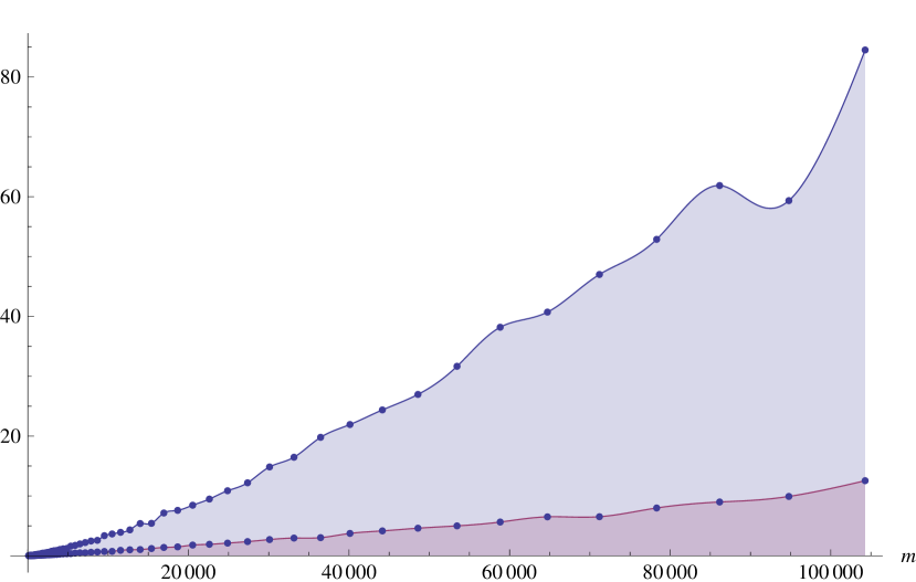
Figure 1: Timings in seconds, measured on a laptop, of Algorithm 1 run at precision $\lambda_{\text{old}}$ (upper curve) and $\lambda_{\text{new}}$ (lower curve) in order to compute an approximation modulo $(5,t^{4m+1})$ of the solution of Equation (4).

Figure 2: Practical speedup obtained with the new precision analysis compared with the theoretical improvement ($m$-axis in logarithmic scale).
($\blacksquare$) ratio $\lambda_{\text{old}}/\lambda_{\text{new}}$; ($\bullet$) actual speedup.

Let us consider the differential equation

$$y^{\prime}=\sqrt{\frac{1+\frac{1}{4}m^{2}y^{2}+m^{6}y^{6}}{1+\frac{1}{4}t^{2}+t^{6}}},\quad y(0)=0,$$ (4)

inspired from algorithms for computing isogenies [3, 9]. Using an implementation in Magma [1] of Algorithm 1, we computed the power series expansion of $y\pmod{5,t^{4m+1}}$ for several $m$. We compared (Figure 1) the CPU time spent on the computation when using on the one hand the precision $\lambda_{\text{new}}=1+\lfloor\log_{5}(4m)\rfloor$, following Theorem 5, and using on the other hand the precision $\lambda_{\text{old}}=1+\mu(4m)=\mathcal{O}(\log(m)^{2})$ found by a straightforward precision analysis — see the discussion in §2 for the definition of $\mu$. For example, with $m=104281$, we compute $\lambda_{\text{old}}=72$ and $\lambda_{\text{new}}=9$. The number of arithmetic operations performed does not depend on the precision $\lambda$, only on $m$, but the number of bit operations does since the base ring for the computation is $\mathbb{Z}/5^{\lambda}\mathbb{Z}$. Thus, the expected speedup is $\lambda_{\text{old}}/\lambda_{\text{new}}$, which is close to what we observed (Figure 2). The implementation is available at https://gist.github.com/lairez/d648b0d7b5392d0fef74.

References

- [1] Wieb Bosma, John Cannon and Catherine Playoust “The Magma algebra system. I. The user language” In J. Symbolic Comput. 24.3-4, 1997, pp. 235–265 DOI: 10.1006/jsco.1996.0125
- [2] Alin Bostan, Laureano González-Vega, Hervé Perdry and Éric Schost “From Newton sums to coefficients: complexity issues in characteristic ” Porto Conte, Italy In Proc. of MEGA, 2005
- [3] Alin Bostan, François Morain, Bruno Salvy and Éric Schost “Fast algorithms for computing isogenies between elliptic curves” In Math. Comput. 77.263, 2008, pp. 1755–1778 DOI: 10.1090/S0025-5718-08-02066-8
- [4] Xavier Caruso, David Roe and Tristan Vaccon “Tracking -adic precision” In LMS J. Comput. Math. 17.suppl. A, 2014, pp. 274–294 DOI: 10.1112/S1461157014000357
- [5] Xavier Caruso, David Roe and Tristan Vaccon “p-Adic Stability In Linear Algebra” Bath, United Kingdom In Proc. of ISSAC ACM, 2015, pp. 101–108 DOI: 10.1145/2755996.2756655
- [6] Bruno Grenet, Joris Hoeven and Grégoire Lecerf “Deterministic root finding over finite fields using Graeffe transforms” In Appl. Algebra Engrg. Comm. Comput., 2015 DOI: 10.1007/s00200-015-0280-5
- [7] Kiran S. Kedlaya and Christopher Umans “Fast polynomial factorization and modular composition” In SIAM J. Comput. 40.6, 2011, pp. 1767–1802 DOI: 10.1137/08073408X
- [8] H. T. Kung “On computing reciprocals of power series” In Numer. Math. 22, 1974, pp. 341–348
- [9] Reynald Lercier and Thomas Sirvent “On Elkies subgroups of -torsion points in elliptic curves defined over a finite field” In J. Théor. Nombres Bordeaux 20, 2008, pp. 783–797
- [10] Arnold Schönhage “Fast parallel computation of characteristic polynomials by Leverrier’s power sum method adapted to fields of finite characteristic” In Automata, languages and programming (Lund, 1993) 700, LNCS Berlin: Springer, 1993, pp. 410–417 DOI: 10.1007/3-540-56939-1_90
- [11] Tristan Vaccon “Précision -adique”, 2015