Dirac monopoles with polar-core vortex induced by spin-orbit coupling in spinor Bose-Einstein condensates

Abstract

We report Dirac monopoles with polar-core vortex induced by spin-orbit coupling in ferromagnetic Bose-Einstein condensates, which are attached to two nodal vortex lines along the vertical axis. These monopoles are more stable in the time scale of experiment and can be detected through directly imaging vortex lines. When the strength of spin-orbit coupling increases, Dirac monopoles with vortex can be transformed into those with square lattice. In the presence of spin-orbit coupling, increasing the strength of interaction can induce a cyclic phase transition from Dirac monopoles with polar-core vortex to those with Mermin-Ho vortex. The spin-orbit coupled Bose-Einstein condensates not only provide a new unique platform for investigating exotic monopoles and relevant phase transitions, but also can preserve stable monopoles after a quadrupole field is turned off.

Dirac monopoles Dirac have attracted more and more attention in a wide area of research including solid state physics Castelnovo ; Morris ; Pollard ; Zhou ; Khomskii ; Bovo , the quantum field Ray ; Ray2 , and other systems Cardoso ; Goddard ; Brekke ; Bakker . In particular, the recent realization of spinor Bose-Einstein condensates (BECs), due to many possible order-parameter manifolds, provides an ideal platform for creating monopoles Martikainen ; Pietila and others topological nontrivial structures Williams ; Hall ; Khawaja ; Choi . So far, both the monopole with one terminating nodal line Ray and the isolated monopole without such nodal line Ray2 have been realized in the BECs. Theoretically, several types of monopoles have been investigated Busch ; Garc ; Stoof ; Savage ; Ruokokoski ; Pietil ; Conduit ; Cho ; Solnyshkov ; Kiffner , including two-dimensional monopoles Busch ; Garc , the monopoles in antiferromagnetic system Stoof , and two-component monopoles Pietil . A majority of studies on monopoles in spinor BECs have been only limited to the systems with spin-dependent interaction. However, spin-orbit (SO) coupling, the interaction between the spin of a quantum particle and its momentum, has not been considered.

The SO coupling in the BECs can be controlled and tuned by using optical fields or a sequence of pulsed homogeneous magnetic fields Lin ; Rus ; Liu1 ; Zhang1 ; Ji ; Campbell ; Lan ; Anderson1 ; Anderson ; Wang1 ; Cheuk , which provides opportunities to search for novel quantum states in BECs Wang ; Su ; Liu ; Xu ; Sinha ; Hu ; Gopalakrishnan ; Li ; Han . These novel quantum states are based on the fact that the SO coupling makes the internal states coupled to their momenta. Meanwhile, due to the SO coupling, the atoms with pseudo-spins are not constrained by fundamental symmetries such as global symmetry and mirror symmetry. This will give rise to the remarkable phenomena not encountered anywhere else in physics. An immediate question is, whether the SO coupling induces unknown types of monopoles that do not have an analogy in the case of spinor BECs without the SO coupling.

In this Letter, we find a new type of monopoles, the Dirac monopoles with the polar-core vortex (M-PCV), induced by the SO coupling in ferromagnetic BECs. Different from the case without the SO coupling Ray ; Pietila , here the monopoles locates at the endpoints of two nodal lines along the vertical axis. Compared with previous work Ray ; Ruokokoski , in this work, the Dirac strings are not observed to split until $22.8$ ms, indicating that M-PCV are more stable and long-lived, which makes the potential experimental observation of such the monopoles easier to be realized. We further demonstrate that the monopoles with the square lattice (M-SL) occur under the strong SO coupling, which can be observed in a wide region of parameters. We find, for the first time, increasing the strength of spin-independent interaction can induce a cyclic phase transition from M-PVC to those with Mermin-Ho vortex (M-MHV) in the presence of weak SO coupling.

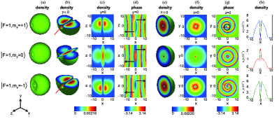
Figure 1: (Color online). (a) Isosurface of particle densities. (b) Particle densities for $y\leq 0$, where the red arrows indicate the location of two nodal lines (Dirac strings). The phenomenon for $x\leq 0$ is the same that for $y\leq 0$. (c) and (d) Densities and phase distributions of the $y=0$ planes, in (d), the phases at both sides of the $y=0$ planes are inverse, which is denoted by the black arrows. (e) Particle densities for $z\leq 0$. (f) and (g) Densities and phase distributions of the $z=0$ planes, the singly vortex is denoted by the black circle of arrow and the singly antivortex is denoted by the red circle of arrow. (h) The one-dimensional density distributions the corresponding (f). Here, the dimensionless SO coupling strength $\kappa=2$, the dimensionless spin-dependent interaction parameter $\lambda_{2}=-75$, the dimensionless spin-independent interaction parameter $\lambda_{0}=7500$, the dimensionless strength of the magnetic field gradient $B_{1}=0.6$, and the isotropic optical trap $\omega_{r}=\omega_{z}=2\pi\times 250$Hz Pietila .

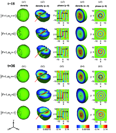
Figure 2: (Color online). Real time evolutions of M-PCV. (a1)-(a5) $t=18$. (b1)-(b5) $t=36$. (a1) and (b1) Isosurface of the particle densities. (a2) and (b2) Particle densities for $y\leq 0$, where the red arrows indicate the location of the nodal lines (Dirac strings). (a3) and (b3) Phase distributions of the $y=0$ planes. Note that the phases at both sides of the $y=0$ planes are inverse, which is denoted by the black arrows. (a4) and (b4) Particle densities for $z\leq 0$. (a5) and (b5) Phase distributions of the $z=0$ planes, the singly vortex is denoted by the black circle of arrow and the singly antivortex is denoted by the red circle of arrow. Here, the real time $t^{\prime}=0.64t$ msec and other parameters are same as in Fig.1.

We consider the monopoles that arise from the three-dimensional spin-1 BECs with a two-dimensional SO coupling Anderson and a controllable magnetic field Ray . In the mean-field approximation, the Hamiltonian for the spin-1 BECs in an optical trap is written as Pietila ; Savage ; Ruokokoski ; Wang ; Pu ; Su ; Liu

$$\begin{split}H\!=\!&\int d^{3}\mathbf{r}\bigg{\{}\mathbf{\Psi}^{\dagger}\left(T\!+\!V_{opt}(\mathbf{r})\!+\!\mathcal{V}_{so}\!+\!g_{F}\mu_{B}\mathbf{B}(\mathbf{r})\cdot\mathcal{F}\right)\mathbf{\Psi}\\ &\!+\!\left(\frac{c_{0}}{2}n^{2}\!+\!\frac{c_{2}}{2}[(n_{1}\!-\!n_{-1})^{2}\!+\!2|\Psi^{\ast}_{1}\Psi_{0}\!+\!\Psi^{\ast}_{0}\Psi_{-1}|^{2}]\right)\bigg{\}},\end{split}$$ (1)

where $\mathbf{\Psi}=[\Psi_{1}(\mathbf{r}),\Psi_{0}(\mathbf{r}),\Psi_{-1}(\mathbf{r})]^{T}$ is the order parameter of the BECs with normalization $\int d^{3}\mathbf{r}\mathbf{\Psi}^{\dagger}\mathbf{\Psi}=N$, and $N$ is the total particle number. The kinetic energy $T=-\hbar^{2}\nabla^{2}/(2m)$. The total particle density is defined by $n=\sum_{m}n_{m}$, wherein $n_{m}=|\Psi_{m}(\mathbf{r})|^{2}$ with $m=0,\pm 1$. The optical trapping potential $V_{opt}(\mathbf{r})=m[\omega^{2}_{r}(x^{2}+y^{2})+\omega^{2}_{z}z^{2}]/2$, where $\omega_{r}$ and $\omega_{z}$ are the radial and axial trapping frequencies, and $m$ is the mass of a ⁸⁷Rb atom. The vector of spin-1 matrices is defined by $\mathcal{F}=(\mathcal{F}_{x},\mathcal{F}_{y},\mathcal{F}_{z})^{T}$, wherein $\mathcal{F}_{x}$, $\mathcal{F}_{y}$ and $\mathcal{F}_{z}$ are the $3\times 3$ Pauli spin-1 matrices. The SO coupling term is written as $\mathcal{V}_{so}=-i\hbar(\kappa_{x}\mathcal{F}_{x}\partial_{x}+\kappa_{y}\mathcal{F}_{y}\partial_{y})$, where $\kappa_{x}$ and $\kappa_{y}$ are the strengths of the SO coupling. We define $\kappa_{x}=\kappa_{y}=\kappa$ for isotropic SO coupling (Rashba-type) and $\kappa_{x}\neq\kappa_{y}$ for anisotropic SO coupling. The external magnetic field is written as $\mathbf{B}(\mathbf{r})=B_{1}^{{}^{\prime}}(x\widehat{e}_{x}+y\widehat{e}_{y})+B_{2}^{{}^{\prime}}z\widehat{e}_{z}$, where the condition $2B_{1}^{{}^{\prime}}+B_{2}^{{}^{\prime}}=0$ must be satisfied according to Maxwell’s equation $\nabla\cdot\mathbf{B}=0$. The Land$\acute{e}$ factor $g_{F}=-1/2$ and $\mu_{B}$ is the Bohr magnetion. For the interaction terms, the coupling parameters are given by $c_{0}=4\pi\hbar^{2}(a_{0}+2a_{2})/3m$ and $c_{2}=4\pi\hbar^{2}(a_{2}-a_{0})/3m$, where $\hbar$ is the Planck constant and $a_{0,2}$ are two-body s-wave scattering lengths for total spin $0,2$. We choose $a_{2}=(100.4\pm 0.1)a_{B}$ for total spin channel $F_{total}=2$ and $a_{0}=(101.8\pm 0.2)a_{B}$ for total spin channel $F_{total}=0$ Stenger ; van ; Stamper-Kurn , where $a_{B}$ is the Bohr radius. The time, the energy, the strength of the SO coupling, and the strength of the magnetic field gradient are scaled by $\omega^{-1}$, $\hbar\omega$, $\sqrt{\hbar\omega/m}$, and $\omega\hbar/(g_{F}\mu_{B}a_{h})$, respectively. The stationary states of the monopoles are obtained (see Supplemental Material sm ) by using the standard imaginary-time propagation combined with finite-difference methods Dalfovo ; Zhang ; Bao . The dynamic evolutions of the monopoles are obtained using the split-operator combined with the Crank-Nicolson method, the time step of dynamic simulation is $10^{-4}/\omega$.

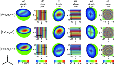
Figure 3: (Color online). (a) Particle densities for $y\leq 0$. (b) Phase distributions of the $y=0$ planes, the phases at both sides of the $y=0$ planes are inverse, which is denoted by the black arrows. (c) Particle densities for $x\leq 0$. (d) Phase distributions of the $x=0$ planes, the phases at both sides of the $x=0$ planes are also inverse, which is denoted by the black arrows. (e) Particle densities for $z\leq 0$. Note that the density distribution in the $x$-$y$ plane ($z=0$) represents square lattice structure. (f) Phase distributions of the $z=0$ planes. Here, $\kappa=16$ and other parameters are same as in Fig.1.

We first study the structures of the monopoles without the SO coupling. A doubly quantized vortex line splits into two singly quantized vortex lines partly in the $m_{F}=+1$ and $-1$ components, because here a homogeneous bias field is not considered in the absence of the SO coupling. The phases of the vortex line along the $z$ and $y$ axes are opposed, which is similar to the vortex-antivortex pair Devreese ; Chibotaru . In fact, the doubly quantized vortex will split into two singly quantized vortices absolutely as the time goes on Shin ; Huhtam . Therefore, we can suppose that the monopole is metastable (M-MS) in the absence of the SO coupling sm . Next, we start to study how the SO coupling gives rise to exotic monopole structures. When the SO coupling is weak, the M-PCV are found. The structures of the M-PCV represent a singly vortex line in the $m_{F}=+1$ component, a soliton in the $m_{F}=0$ component and a singly antivortex line in the $m_{F}=-1$ component (Fig. 1). Compared with the monopoles in BECs without the SO coupling Ray ; Pietila , in the present system, there exists two monopoles located at the endpoints of two nodal lines along the vertical axis [as highlighted by the red arrows in Fig. 1(b)], which is believed to be caused by the interaction of the spin of a particle with its motion. Meanwhile, being different from the monopoles in spin ices Castelnovo ; Morris ; Pollard ; Zhou ; Khomskii ; Bovo , our results demonstrate the fundamental quantum features and topological structures of the monopoles predicted by Dirac Dirac . A topological defect has a longer lifetime, which is beneficial for its experimental observation. Therefore, we perform the dynamic simulations for the M-PCV. The simulations show that the structures of the monopoles keep the original shape (Fig. 1) from $t=18$ to $t=36$ [Figs. 2(a1)-2(b5)]. Especially, the nodal lines are not expanded and still exist in the condensates [Figs. 2(a2) and 2(b2)]. Furthermore, during the dynamic evolution, as seen in the phase profile of the wave function in the $z=0$ plane, the singly vorticity is well maintained and no vortex splitting is observed [Figs. 2(a5) and 2(b5)]. Compared with the dynamics of the monopoles in the absence of the SO coupling Ray , where the doubly quantized vortex splits into two singly vortices after roughly $10ms$. In our case, the quantized vortex is not observed to split until $t=36$ ($22.8ms$), confirming that the M-PCV are more stable in the time scale of experiment. Therefore, we can expect that the experimental observation of such monopoles should be more practical in the case of the SO coupling. In addition, the dynamics of the monopoles are also stable after the magnetic field is turned off, which suggests that the SO coupling can preserve stable monopoles sm .

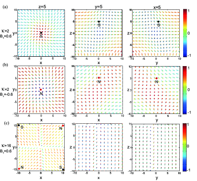
Figure 4: (Color online). (a) Spin textures of M-PCV describe the south magnetic poles (the black dot S). (b) Spin textures of the antimonopoles describe the north magnetic poles (the red dot N). (c) Spin textures of M-SL represent spin configurations of the south magnetic poles (the black dot S) and north magnetic poles (the red dot N). Other parameters are same as in Fig.1.

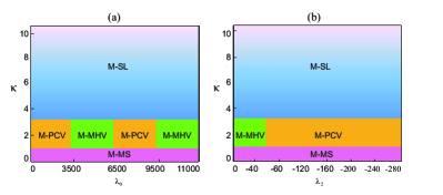
Figure 5: (Color online). (a) Phase diagram of the monopole with $\kappa$ and $\lambda_{0}$ for a given $\lambda_{2}$. (b) Phase diagram of the monopole with $\kappa$ and $\lambda_{2}$ for a given $\lambda_{0}$.

We also demonstrate that the M-PCV can occur in the presence of the oblate trap sm . The influence of the magnetic field gradient on the monopoles is also investigated sm . In order to identify the effect of the interaction on the monopoles, we also perform the simulations that decrease $\lambda_{2}$ for a given $\kappa$. The simulations show that the M-MHV is obtained, which represents a soliton in the $m_{F}=+1$ component, a singly vortex line in the $m_{F}=0$ component and a doubly quantized vortex line in the $m_{F}=-1$ component Mizushima . This result shows that such the monopole structure can exist in the condensates not only without SO coupling Ray ; Pietila , but also with SO coupling sm . When the SO coupling strength increases, the M-SL are found, as shown in Figs. 3(a)-3(f). The square lattice in the central zone is very distinct, as compared with that in the surrounding zone. Meanwhile, the density distribution in the longitudinal direction is of the stripe structure. More importantly, the M-SL are not affected by the interactions, because the lowest-energy state is not affected by the interactions for the strong SO coupling. Meanwhile, the antimonopoles emerge in the system, which suggests that the periodic magnetic monopole can occur in the presence of strong SO coupling. Finally, we also consider an anisotropic SO coupling case, which shows that the monopole vanishes. Because the Dirac string can be removed in the presence of asymmetric SO coupling sm .

The spinor BECs can be considered as a magnetic system, which reflects physical properties of topological defects Stamper-Kurn . We therefore study topological spin textures of the monopoles. the components of the spin vector are given by $F_{x}=\frac{1}{\sqrt{2}}[\psi_{1}^{\ast}\psi_{0}+\psi_{0}^{\ast}(\psi_{1}+\psi_{-1})+\psi_{-1}^{\ast}\psi_{0}]$, $F_{y}=\frac{i}{\sqrt{2}}[-\psi_{1}^{\ast}\psi_{0}+\psi_{0}^{\ast}(\psi_{1}-\psi_{-1})+\psi_{-1}^{\ast}\psi_{0}]$, and $F_{z}=|\psi_{1}|^{2}-|\psi_{-1}|^{2}$ Su ; Liu ; Mizushima ; Kasamatsu ; Kawakami ; Mizushima2 ; Kasamatsu2 . The spin textures of the M-PCV are shown in Fig. 4(a). The spin aligns with the radially inward hedgehog distribution in the $x$-$y$ plane, representing the spin texture of a south magnetic pole, while the spin textures in the $x$-$z$ and $y$-$z$ planes show the cross hyperbolic distribution Mizushima2 ; Kita . It has been shown that in the absence of the SO coupling, the spin texture shows the north magnetic pole Ruokokoski . In our case, the SO coupling changes the spin direction, which leads to the fact that the north magnetic pole can be transformed into the south magnetic pole. As shown in Fig. 4(b), the spin textures of the antimonopoles are observed, which represents the north magnetic poles. For the case of the strong SO coupling, as shown in Fig. 4(c), the spin textures are divided into four portions in the $x$-$y$ plane. The spin texture behaves as the ferromagnetic distribution at each portion. The spin orientations at two diagonal portions are opposite, which reflects the structures of monopoles and antimonopoles that locate in the boundaries of the condensates. The spin textures in the $x$-$z$ and $y$-$z$ planes form the spin stripe. In addition, the spin texture in the case of the anisotropic SO coupling is also investigated sm . Finally, we further prove that the M-PCV are stable through the dynamic evolution of the spin texture sm .

We now consider the interplay between the SO coupling and the interaction, due to the coupling of the spin of a particle with its motion induced by magnetic pulses and the transformation of magnetic order induced by the interaction, which leads to the rich phase diagrams of the monopoles. For a given $\lambda_{2}$ being -75, the phase diagram as functions of $\kappa$ and $\lambda_{0}$ is shown in Fig. 5(a). The monopole is metastable when $\kappa$ is less than a critical value $\kappa_{c}=0.8$. For $0.8<\kappa\leq 3$, the M-PCV exist when $0<\lambda_{0}\leq 3000$ and $5000<\lambda_{0}\leq 8000$, while the M-MHV emerge when $3000<\lambda_{0}\leq 5000$ and $8000<\lambda_{0}\leq 11000$. This indicates that a cyclic phase transition from the M-PCV to the M-MHV can occur with the increasing $\lambda_{0}$. Note that if there is no the SO coupling, such the cyclic phase transition will not occur. The M-SL occur when $\kappa>3$, confirming that at strong SO coupling the monopoles are not affected by the interactions and can exist in the wide parameter region. Furthermore, the phase diagram as functions of $\kappa$ and $\lambda_{2}$ for a given $\lambda_{0}$ being 7500 is shown in Fig. 5(b). For $0.8<\kappa\leq 3$, there exists the M-MHV when $\lambda_{2}$ is less than 60, while the M-PCV emerge when $\lambda_{2}$ is more than 60. This result suggests that the increasing the spin-dependent interaction only leads to the direct phase transition from the M-MHV to M-PCV.

We finally briefly discuss the experimental feasibility of creating the monopoles in SO coupled BECs (see Supplemental Material sm ). We consider spin-1 BECs of alkali ⁸⁷Rb atoms, where particle number $N\approx 0.6(1.8)\times 10^{5}$. First of all, a quadrupole field is applied and turned on, which is realized by a pair of Helmholtz coils. Then, when a point source of the superfluid flow is formed Pietila , the quadrupole field is turned off. The pulsed magnetic fields are turned on, which creates two-dimensional SO coupling Anderson . We take some parameters from the recent experiments Ray ; Pietila ; Anderson , which includes the isotropic optical trap $\omega_{r}=\omega_{z}=2\pi\times 250$Hz, the anisotropic optical trap $\omega_{r}\approx 2\pi\times 160$ Hz and $\omega_{z}\approx 2\pi\times 220$ Hz, the constant bias magnetic field $B^{(0)}=20$G, and the quadrupole field gradient $B_{1}^{{}^{\prime}}=0.03\sim 0.1$ T/m. For the M-PCV, the SO coupling strength $\kappa\sim 0.8-3$. We find the dynamic period of the monopoles $t^{\prime}\sim 11ms$ , which is much shorter than the lifetime of the BECs and can be observed stably in experiments.

In conclusion, we have shown that the weak SO coupling leads to the emergence of the M-PCV that are stable and long-lived, and the strong SO coupling leads to the emergence of the M-SL in spinor BECs. We have predicted the rich phase diagrams of the monopoles by changing the SO coupling strength, the spin-dependent interaction, and the spin-independent interaction. Such monopoles can be proved by means of imaging the vortex lines in a real experiment. This work paves the way for future explorations of the monopole with respect to gauge field, topological defects and the corresponding dynamical stability in quantum systems.

I Supplementary Material

In this supplementary material, we present the details on calculation of the stationary states with respect to the monopoles, experimental setup of creating the monopoles in spin-orbit (SO) coupled Bose-Einstein condensates (BECs), the structures of the monopoles in the absence of the SO coupling, the monopoles with the Mermin-Ho vortex (M-MHV), the effect of the anisotropic optical trap on the monopoles, the effect of the quadrupole field gradient on the monopoles, ground states for the anisotropic SO coupling, spin textures for the anisotropic SO coupling, the dynamic evolution of the monopoles in the absence of the quadrupole field, and the dynamic evolution of the spin texture.

Calculation of the stationary states with respect to the monopoles

We investigate the stationary states of the monopoles in the SO coupled spinor BECs , which is based on the Gross-Pitaevskii mean-field theory. The wave functions of spin-1 BECs are formulated as the dimensionless coupled Gross-Pitaevskii equations 1 ; 2 ; 3 ; 4 ; 7 ; 5 ; 6

$$\begin{split}i\frac{\partial\psi_{1}}{\partial t}=&(-\frac{1}{2}\nabla^{2}+V+\lambda_{0}\rho+\lambda_{2}(\rho_{1}+\rho_{0}-\rho_{-1})+B_{2}z)\psi_{1}\\ &+B_{1}(x-iy)\psi_{0}+\kappa(-i\partial_{x}-\partial_{y})\psi_{0}+\lambda_{2}\psi^{\ast}_{-1}\psi_{0}^{2},\end{split}$$ (2)

$$\begin{split}i\frac{\partial\psi_{0}}{\partial t}=&(-\frac{1}{2}\nabla^{2}+V+\lambda_{0}\rho+\lambda_{2}(\rho_{1}+\rho_{-1}))\psi_{0}\\ &+B_{1}(x+iy)\psi_{1}+B_{1}(x-iy)\psi_{-1}+\kappa(-i\partial_{x}+\partial_{y})\psi_{1}\\ &+\kappa(-i\partial_{x}-\partial_{y})\psi_{-1}+2\lambda_{2}\psi_{1}\psi_{-1}\psi_{0}^{\ast},\end{split}$$ (3)

$$\begin{split}i\frac{\partial\psi_{-1}}{\partial t}=&(-\frac{1}{2}\nabla^{2}+V+\lambda_{0}\rho+\lambda_{2}(\rho_{0}+\rho_{-1}-\rho_{1})-B_{2}z)\psi_{-1}\\ &+B_{1}(x+iy)\psi_{0}+\kappa(-i\partial_{x}+\partial_{y})\psi_{0}+\lambda_{2}\psi_{1}^{\ast}\psi_{0}^{2},\end{split}$$ (4)

where the dimensionless wave function $\psi_{j}=N^{-1/2}a_{h}^{3/2}\Psi_{j}$ $(j=1,0,-1)$ and the total condensate density $\rho=\rho_{1}+\rho_{0}+\rho_{-1}$ with $\rho_{j}=|\psi_{j}|^{2}$ $(j=1,0,-1)$. The dimensionless optical trapping potential $V(\mathbf{r})=\frac{1}{2}(\gamma_{r}^{2}x^{2}+\gamma_{r}^{2}y^{2}+\gamma_{z}^{2}z^{2})$ with $\gamma_{r}=\omega_{r}/\omega$, $\gamma_{z}=\omega_{z}/\omega$ and $\omega=min\{\omega_{r},\omega_{z}\}$. The dimensionless interaction strengths $\lambda_{0}=4\pi N(a_{0}+2a_{2})/3a_{h}$ and $\lambda_{2}=4\pi N(a_{2}-a_{0})/3a_{h}$, where $\hbar$ is the Planck constant and $a_{0,2}$ are two-body s-wave scattering lengths for total spin $0,2$. The characteristic length of the harmonic trap is defined as $a_{h}=\sqrt{\hbar/m\omega}$. The dimensionless strength of the magnetic field gradient complies the condition $2B_{1}+B_{2}=0$. The time, the energy, the strength of the SO coupling, and the strength of the magnetic field gradient are scaled by $\omega^{-1}$, $\hbar\omega$, $\sqrt{\hbar\omega/m}$, and $\omega\hbar/(g_{F}\mu_{B}a_{h})$, respectively.

The stationary state wave functions of the monopoles are obtained by using the standard imaginary-time propagation, which is combined with the second-order centered finite-difference discretization and the backward/forward Euler methods. By applying the transformation relation $t\rightarrow\tau=-\mathrm{i}t$, the imaginary time evolution equations are expressed as follows:

$$\begin{split}\frac{\partial\psi_{1}}{\partial t}=&(\frac{1}{2}\nabla^{2}-V-\lambda_{0}\rho-\lambda_{2}(\rho_{1}+\rho_{0}-\rho_{-1})-B_{2}z)\psi_{1}\\ &-B_{1}(x-iy)\psi_{0}-\kappa(-i\partial_{x}-\partial_{y})\psi_{0}-\lambda_{2}\psi^{\ast}_{-1}\psi_{0}^{2},\end{split}$$ (5)

$$\begin{split}\frac{\partial\psi_{0}}{\partial t}=&(\frac{1}{2}\nabla^{2}-V-\lambda_{0}\rho-\lambda_{2}(\rho_{1}+\rho_{-1}))\psi_{0}\\ &-B_{1}(x+iy)\psi_{1}-B_{1}(x-iy)\psi_{-1}-\kappa(-i\partial_{x}+\partial_{y})\psi_{1}\\ &-\kappa(-i\partial_{x}-\partial_{y})\psi_{-1}-2\lambda_{2}\psi_{1}\psi_{-1}\psi_{0}^{\ast},\end{split}$$ (6)

$$\begin{split}\frac{\partial\psi_{-1}}{\partial t}=&(\frac{1}{2}\nabla^{2}-V-\lambda_{0}\rho-\lambda_{2}(\rho_{0}+\rho_{-1}-\rho_{1})+B_{2}z)\psi_{-1}\\ &-B_{1}(x+iy)\psi_{0}-\kappa(-i\partial_{x}+\partial_{y})\psi_{0}-\lambda_{2}\psi_{1}^{\ast}\psi_{0}^{2},\end{split}$$ (7)

in addtion, the average energy of the system is expressed as follows:

$$\begin{split}E(\psi_{1},\psi_{0},\psi_{-1})=&\int_{\Omega}\bigg{\{}\sum_{m=0,\pm 1}\psi_{m}^{\ast}h_{d}\psi_{m}+\frac{\lambda_{0}}{2}\rho^{2}+\frac{\lambda_{2}}{2}(\rho_{1}+\rho_{0}-\rho_{-1})\rho_{1}\\ &+\frac{\lambda_{2}}{2}(\rho_{1}+\rho_{-1})\rho_{0}+\frac{\lambda_{2}}{2}(\rho_{0}+\rho_{-1}-\rho_{1})\rho_{-1}\\ &+\lambda_{2}(\psi_{-1}^{\ast}\psi_{0}^{2}\psi_{1}^{\ast}+\psi_{-1}{\psi_{0}^{\ast}}^{2}\psi_{1})+B_{2}z(\rho_{1}-\rho_{-1})\\ &+B_{1}(x-\mathrm{i}y)(\psi_{1}^{\ast}\psi_{0}+\psi_{0}^{\ast}\psi_{-1})+B_{1}(x+\mathrm{i}y)(\psi_{0}^{\ast}\psi_{1}+\psi_{-1}^{\ast}\psi_{0})\\ &+\kappa[\psi_{1}^{\ast}(-\mathrm{i}\partial_{x}-\partial_{y})\psi_{0}+\psi_{0}^{\ast}(-\mathrm{i}\partial_{x}+\partial_{y})\psi_{1}\\ &+\psi_{0}^{\ast}(-\mathrm{i}\partial_{x}-\partial_{y})\psi_{-1}+\psi_{-1}^{\ast}(-\mathrm{i}\partial_{x}+\partial_{y})\psi_{0}]\bigg{\}}d\Omega.\end{split}$$ (8)

In order to solve equations (6)-(8), we use second-order centered finite-difference for the spatial discretization and the backward/forward Euler scheme to solve the corresponding linear/nonlinear terms for the time discretization. The periodic boundary condition is considered, the computational grids are 120$\times$120$\times$120 that corresponds to the volume 20$\times$20$\times$20 in the units of $a_{h}^{3}$, and the scale for three dimension system is $34.2\mu m\times 34.2\mu m\times 34.2\mu m$. A initial trial state of the normalized random number of complex-values is given. The final steady states are not depend on the initial trial wave function. The average energy decays monotonically with time until the steady states are reached.

Experimental setup of creating the monopoles in spin-orbit coupled Bose-Einstein condensates

The experimental setup is shown schematically in Fig. 6(a). We consider spin-1 BECs of alkali ⁸⁷Rb atoms, where the ⁸⁷Rb BECs contain about $N\approx 0.6(1.8)\times 10^{5}$ atoms. First of all, a quadrupole field is applied and turned on, which is realized by a pair of Helmholtz coils. The strength of the magnetic field is zero at the center of the quandrupole field, which corresponds to a point source of the superfluid flow. The superfluid flow of the spinor condensates can be characterized by its vorticity $\Omega_{s}=\hbar\hat{\mathbf{e}}_{r^{\prime}}/(mr^{\prime 2})$, where $r^{\prime}$ is the sphere radius. The vorticity $\Omega_{s}$ is equivalent to the magnetic field of a monopole that distributes radially outward in a hedgehog form. A monopole can be considered as a point source of the superfluid flow 1 . Then, when a point source of the superfluid flow is formed, the quadrupole field is turned off. The pulsed magnetic fields are turned on, which creates two-dimensional SO coupling 8 . The cloud of atoms is situated 50$\mu m$ above the surface of the atom chip. A constant bias magnetic field $B^{(0)}\mathbf{e}_{z}$ is applied out of plane, which leads to splitting of the magnetic sublevels. Two pairs of microwires parallel to $\mathbf{e}_{x}$ and $\mathbf{e}_{y}$ provide the rf magnetic fields $\mathbf{B}_{x}(\mathbf{r},t)$ and $\mathbf{B}_{y}(\mathbf{r},t)$. In the first stage $(0\leq t<\tau)$, the rf magnetic field $\mathbf{B}_{x}(\mathbf{r},t)$ with the frequency $\omega_{1}$ leads to an effective coupling vector in the $x$ direction and a spin-dependent phase gradient in the $y$ direction, where the SO coupling is written as $-i\hbar\kappa_{x}\mathcal{F}_{x}\partial_{x}$. In the second stage $(\tau\leq t<2\tau)$, the rf magnetic field $\mathbf{B}_{y}(\mathbf{r},t)$ with frequency $\omega_{2}$ leads to an effective coupling vector in the $y$ direction and a spin-dependent phase gradient in the $x$ direction, where the SO coupling is written as $-i\hbar\kappa_{y}\mathcal{F}_{y}\partial_{y}$. When the rf magnetic fields both $\mathbf{B}_{x}(\mathbf{r},t)$ and $\mathbf{B}_{y}(\mathbf{r},t)$ are applied, the two-dimensional SO coupling is created, which is written as $\mathcal{V}_{so}=-i\hbar(\kappa_{x}\mathcal{F}_{x}\partial_{x}+\kappa_{y}\mathcal{F}_{y}\partial_{y})$ in the first-order approximation for a sufficiently short duration $\tau$. The strengths of the SO coupling $\kappa_{x}$ and $\kappa_{y}$ are determined by the strengths of the magnetic field gradient of $\mathbf{B}_{x}(\mathbf{r},t)$ and $\mathbf{B}_{y}(\mathbf{r},t)$. Due to the SO coupling, the spin degeneracy of three-component bosons is lifted and the free particle energy spectrum splits into three energy branches with different helicity [Fig. 6(b)]. The Rashba ring can be seen from the minimum energy spectrum, which is denoted by the black circular ring in Fig. 6(b). We take some parameters from the recent experiments 9 ; 1 ; 8 , which includes the isotropic optical trap $\omega_{r}=\omega_{z}=2\pi\times 250$Hz, the anisotropic optical trap $\omega_{r}\approx 2\pi\times 160$ Hz and $\omega_{z}\approx 2\pi\times 220$ Hz, the constant bias magnetic field $B^{(0)}=20$G, and the quadrupole field gradient $B_{1}^{{}^{\prime}}=0.03\sim 0.1$ T/m.

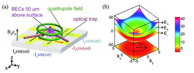
Figure 6: (Color online). Experimental setup of creating the monopoles in SO coupled BECs. (a) Experimental geometry of creating the quadrupole field and the SO coupling. A pair of Helmholtz coils are used for creating the quadrupole fields, where the pink particles represent ⁸⁷Rb atoms and the kermesinus arrows show beam paths of the optical trap. The pulsed magnetic field are used for creating the SO coupling, where the cloud of atoms is located 50$\mu m$ above the surface of an atom chip. A bias field $B_{0}$ along the $z$ axis induces the magnetic splitting. Two pairs of parallel microwires are embedded in the atom chip, which produces the amplitude modulated rf field along $x$ and $y$ axis, respectively, these two effective coupling vectors in $x$-$y$ plane induce effective two-dimensional SO coupling in the first-order approximation to short enough duration. (b) Energy spectrum. The single-particle energy spectrum of the monopole with SO coupling strength $\kappa=2$ in $k_{x}-k_{y}$ plane is divided into three branches $E_{+}$, $E_{0}$ and $E_{-}$, the black circular ring represents the Rashba ring from the minimum energy spectrum.

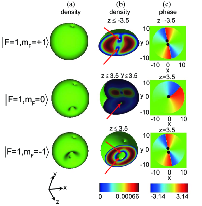
Figure 7: (Color online). The monopole is metastable, a doubly vortex line has split to two singly vortex lines partly, as denoted by the red arrows, where the SO coupling strength $\kappa=0$, the spin-dependent interaction parameter $\lambda_{2}=-75$, the spin-independent interaction parameter $\lambda_{0}=7500$, the strength of the magnetic field gradient $B_{1}=0.6$, and the optical trap frequencies $\omega_{r}=\omega_{z}=2\pi\times 250$Hz. (a) Isosurface of the particle densities. (b) Segments of the isosurface of the particle densities. (c) Phase distributions of slice planes, the black dots indicate the locations of vortices. The unit of the length is $\sqrt{\hbar/m\omega}$, the unit of the strength of the magnetic field gradient is $\omega\hbar/(g_{F}\mu_{B}a_{h})$, the unit of the SO coupling strength is $\sqrt{\hbar\omega/m}$, and the scale for three dimension system is $34.2\mu m\times 34.2\mu m\times 34.2\mu m$.

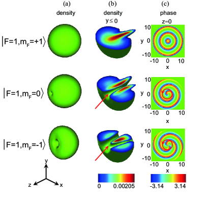
Figure 8: (Color online). The M-MHV are obtained, which behave as a soliton in the $m_{F}=+1$ component, a vortex line with unit circulation in the $m_{F}=0$ component, and a doubly quantized vortex line in the $m_{F}=-1$ component, where the SO coupling strength $\kappa=2$, the spin-dependent interaction parameter $\lambda_{2}=-15$, the spin-independent interaction parameter $\lambda_{0}=7500$, the strength of the magnetic field gradient $B_{1}=0.6$, and the optical trap frequencies $\omega_{r}=\omega_{z}=2\pi\times 250$Hz. (a) Isosurface of the particle densities. (b) Segments of the isosurface of the particle densities ($y\leq 0$), where the red arrows indicate the location of the one nodal line (Dirac string). (c) Phase distributions of the $z=0$ slice planes, the circulations of the single vortex (the second line) and the a doubly vortex (the third line) are the same, which is denoted by the black circles. The unit of the length is $\sqrt{\hbar/m\omega}$, the unit of the strength of the magnetic field gradient is $\omega\hbar/(g_{F}\mu_{B}a_{h})$, the unit of the SO coupling strength is $\sqrt{\hbar\omega/m}$, and the scale for three dimension system is $34.2\mu m\times 34.2\mu m\times 34.2\mu m$.

The structures of the monopoles in the absence of the spin-orbit coupling

Fig. 7 shows the results of the monopoles in the absence of the SO coupling, where the dimensionless SO coupling strength $\kappa=0$, the dimensionless spin-dependent interaction parameter $\lambda_{2}=-75$, the dimensionless spin-independent interaction parameter $\lambda_{0}=7500$, the dimensionless strength of the magnetic field gradient $B_{1}=0.6$, and the optical trap $\omega_{r}=\omega_{z}=2\pi\times 250$ Hz 1 . Note that a doubly quantized vortex line partly splits into two singly quantized vortex lines in the $m_{F}=+1$ and $-1$ components [as highlighted by the red arrow in Fig. 7(b)]. In Ref. 9 , the external magnetic field of the monopole creation is the combination of the quadrupole field and the homogeneous bias field, the vortex lines are located in the direction of the bias field. However, in our case, a homogeneous bias field is not considered in the experimental setup of the monopole creation, which gives rise to the splitting of the doubly quantized vortex line. The structures of the vortex lines for the $m_{F}=+1$ and $-1$ components are similar. The vortex lines for the $m_{F}=+1$ component locate in the part of $z<0$, the vortex lines for the $m_{F}=-1$ component locate in the part of $z>0$, and such the vortex lines extend outwords along the $\pm y$ directions to the boundary of the BECs. The phases at both sides of the vortex line are the same. For the case of the $m_{F}=0$ component, the two vortex lines in the $x=0$ plane cross each other and topologically invariant winding number is 1. The phases of the vortex line along the $z$ and $y$ axes are opposed, being similar to the vortex-antivortex pair 10 ; 11 . In fact, the doubly quantized vortex will split into two singly quantized vortices absolutely as the time goes on 12 ; 13 . Therefore, the results suggest that the monopole is metastable in the absence of the SO coupling.

The monopoles with the Mermin-Ho vortex

In this section, the spin-dependent interaction parameter $\lambda_{2}=-15$, the SO coupling strength $\kappa=2$, the other parameters are chosen as the same with those given for Fig. 7. The M-MHV 14 are obtained, as shown in Fig. 8. The structure of the M-MHV represents a soliton in the $m_{F}=+1$ component, a singly vortex line in the $m_{F}=0$ component and a doubly quantized vortex line in the $m_{F}=-1$ component. The vortices in the $m_{F}=0$ and $m_{F}=-1$ components have the same phase winding direction, which is denoted by the black circles [Fig. 8(C)]. The phases at both sides of $x=0$ and $y=0$ slice planes are inverse. Such the structure of the monopole also emerges in spinor BECs with a magnetic field 9 . Our results show that the M-MHV can exist in the spinor BECs with non-Abelian gauge field.

The effect of the anisotropic optical trap on the monopoles

We also investigate the monopole structures for an anisotropic optical trap, where $\kappa=2$, $\lambda_{2}=-75$, $B_{1}=0.6$, and $\lambda_{0}=7500$. For comparison, we first consider the isotropic optical trap with $\omega_{r}=\omega_{z}=2\pi\times 250$ Hz 1 , as shown in Figs. 9(a1)-9(a3). The monopoles with the polar-core vortex (M-PCV) are obtained. The monopoles behave as a singly vortex line in the $m_{F}=+1$ component, a soliton in the $m_{F}=0$ component, and a singly antivortex line in the $m_{F}=-1$ component. In Figs. 9(b1)-9(b3), the trapping frequencies are given by $\omega_{r}\approx 2\pi\times 160$ Hz and $\omega_{z}\approx 2\pi\times 220$ Hz 9 , and the corresponding the anisotropy parameters related to the optical trap $\gamma_{r}=1$ and $\gamma_{z}=1.375$. We can find that the M-PCV disappear, and at the same time Dirac string embedded in the BECs splits into two strings with a singly quantized vortex. In this case, our results suggest that this anisotropic trapping potential leads to the metastable monopole states. In fact, the M-PCV exist in the condensates when the anisotropy of the optical trap is small, being less than the magnitude of $\gamma_{r}=1$ and $\gamma_{z}=1.375$. In Figs. 9(c1)-9(c3), the trapping frequencies are given by $\omega_{r}\approx 2\pi\times 160$ Hz and $\omega_{z}\approx 2\pi\times 320$ Hz, and the anisotropy parameters related to the optical trap $\gamma_{r}=1$ and $\gamma_{z}=2$. We observe that the M-PCV still exist in the BECs. The results confirm that the M-PCV can occur in the presence of the oblate trap.

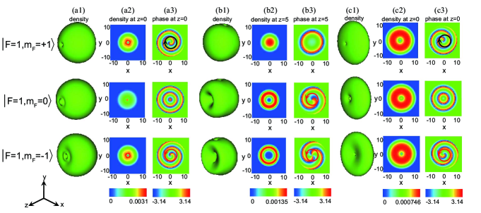
Figure 9: (Color online). The monopole states for the anisotropic trap as obtained by using the strength of the magnetic field gradient $B_{1}=0.6$, the spin-independent interaction parameter $\lambda_{0}=7500$, the spin-dependent interaction parameter $\lambda_{2}=-75$ and the SO coupling strength $\kappa=2$. (a1)-(a3) The optical trap frequencies are given by $\omega_{r}=\omega_{z}=2\pi\times 250$Hz, the anisotropy parameters related to the optical trap $\gamma_{r}=\gamma_{z}=1$, the M-PCV are obtained. (b1)-(b3) The optical trap frequencies are given by $\omega_{r}\approx 2\pi\times 160$Hz and $\omega_{z}\approx 2\pi\times 220$Hz, the anisotropy parameters related to the optical trap $\gamma_{r}=1$ and $\gamma_{z}=1.375$, the M-PCV disappear. (c1)-(c3) The optical trap frequencies are given by $\omega_{r}\approx 2\pi\times 160$Hz and $\omega_{z}\approx 2\pi\times 320$Hz, the anisotropy parameters related to the optical trap $\gamma_{r}=1$ and $\gamma_{z}=2$, the M-PCV remain exist in the system. (a1), (b1) and (c1) show the isosurface of the particle densities. (a2), (b2) and (c2) display the particle densities of the slice planes. (a3), (b3) and (c3) show the phase distributions of the slice planes. The vortex and antivortex are denoted by the black circle of arrow and the red circle of arrow. The unit of the length is $\sqrt{\hbar/m\omega}$, the unit of the strength of the magnetic field gradient is $\omega\hbar/(g_{F}\mu_{B}a_{h})$, the unit of the SO coupling strength is $\sqrt{\hbar\omega/m}$, and the scale for three dimension system is $34.2\mu m\times 34.2\mu m\times 34.2\mu m$.

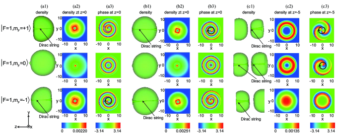
Figure 10: (Color online). The monopole states for different quadrupole field as obtained by using the optical trap frequencies $\omega_{r}=\omega_{z}=2\pi\times 250$Hz, where the spin-independent interaction parameter $\lambda_{0}=7500$, the spin-dependent interaction parameter $\lambda_{2}=-75$, and the SO coupling strength $\kappa=2$. (a1)-(a3) The strength of the magnetic field gradient $B_{1}=-0.6$, the structure of the antimonopole is as follows: a singly antivortex line in the $m_{F}=1$ component, a soliton in the $m_{F}=0$ component, and a singly vortex line in the $m_{F}=-1$ component. (b1)-(b3) The strength of the magnetic field gradient $B_{1}=0.2$, the structure of the monopole is as follows: a singly vortex line in the $m_{F}=1$ component, a soliton in the $m_{F}=0$ component, and a singly antivortex line in the $m_{F}=-1$ component. (c1)-(c3) The strength of the magnetic field gradient $B_{1}=3.8$, the M-PCV disappear. (a1), (b1) and (c1) show the isosurface of the particle densities, Dirac strings are denoted by the black arrows. (a2), (b2) and (c2) show the particle densities of the slice planes. (a3), (b3) and (c3) show the phase distributions of the slice planes. The vortex and antivortex are denoted by the black circle of arrow and the red circle of arrow. The unit of the length is $\sqrt{\hbar/m\omega}$, the unit of the strength of the magnetic field gradient is $\omega\hbar/(g_{F}\mu_{B}a_{h})$, the unit of the SO coupling strength is $\sqrt{\hbar\omega/m}$, and the scale for three dimension system is $34.2\mu m\times 34.2\mu m\times 34.2\mu m$.

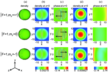
Figure 11: (Color online). (a) Isosurface of the particle densities of the three spin components, where the anisotropic SO coupling $\kappa_{x}=8$ and $\kappa_{y}=2$, the spin-dependent interaction parameter $\lambda_{2}=-75$, the spin-independent interaction parameter $\lambda_{0}=7500$, the strength of the magnetic field gradient $B_{1}=0.6$, the optical trap frequencies $\omega_{r}=\omega_{z}=2\pi\times 250$Hz. (b) and (c) Densities and phase distributions of the stripe phase in the $x$-$y$ plane ($z=0$), the phenomena in the $x$-$z$ plane are similar to those in the $x$-$y$ plane. In (c), we can see that the phases at both sides of the $z=0$ slice plane are inverse, which is indicated by the black arrows. (d) and (e) Densities and phase distributions of the plane wave phase in the $y$-$z$ plane ($x=0$). The unit of the length is $\sqrt{\hbar/m\omega}$, the unit of the strength of the magnetic field gradient is $\omega\hbar/(g_{F}\mu_{B}a_{h})$, the unit of the SO coupling strength is $\sqrt{\hbar\omega/m}$, and the scale for three dimension system is $34.2\mu m\times 34.2\mu m\times 34.2\mu m$.

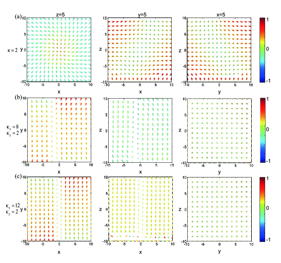
Figure 12: (Color online). (a) When the SO coupling $\kappa_{x}=\kappa_{y}=\kappa=2$, we obtain the spin textures of the M-PCV in the slice planes of $z=5$, $y=5$ and $x=5$. (b) When the SO coupling $\kappa_{x}=8$ and $\kappa_{y}=2$, the spin textures show the stripe distribution in the $z=5$ and $y=5$ planes and the plane wave ferromagnetic distribution in the $x=5$ plane. (c) When the SO coupling $\kappa_{x}=12$ and $\kappa_{y}=2$, the spin textures are similar to those in (b). For all figures, the strength of the magnetic field gradient $B_{1}=0.6$, the spin-dependent interaction parameter $\lambda_{2}=-75$, the spin-independent interaction parameter $\lambda_{0}=7500$, the optical trap frequencies $\omega_{r}=\omega_{z}=2\pi\times 250$Hz, the unit of the length is $\sqrt{\hbar/m\omega}$, the unit of the strength of the magnetic field gradient is $\omega\hbar/(g_{F}\mu_{B}a_{h})$, the unit of the SO coupling strength is $\sqrt{\hbar\omega/m}$, and the scale for three dimension system is $34.2\mu m\times 34.2\mu m\times 34.2\mu m$.

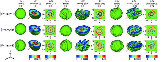
Figure 13: (Color online). The dynamics of the M-PCV remain stable when the quadrupole field is turned off, where the weak SO coupling strength $\kappa=2$, the spin-dependent interaction parameter $\lambda_{2}=-75$, spin-independent interaction parameter $\lambda_{0}=7500$, the optical trap frequencies $\omega_{r}=\omega_{z}=2\pi\times 250$Hz, and the real time $t^{\prime}=0.64t$ msec. (a1)-(a3) t=0. (b1)-(b3) t=6. (c1)-(c3) t=12. (a1), (b1) and (c1) Isosurface of the particle densities. (a2), (b2) and (c2) Particle densities for $y\leq 0$, where the red arrows indicate the location of the nodal lines (Dirac strings). (a3), (b3) and (c3) Phase distributions of the $z=0$ slice planes, the singly vortex is denoted by the black circle of arrow and the singly antivortex is denoted by the red circle of arrow. The unit of the length is $\sqrt{\hbar/m\omega}$, the unit of the strength of the magnetic field gradient is $\omega\hbar/(g_{F}\mu_{B}a_{h})$, the unit of the SO coupling strength is $\sqrt{\hbar\omega/m}$, and the scale for three dimension system is $34.2\mu m\times 34.2\mu m\times 34.2\mu m$.

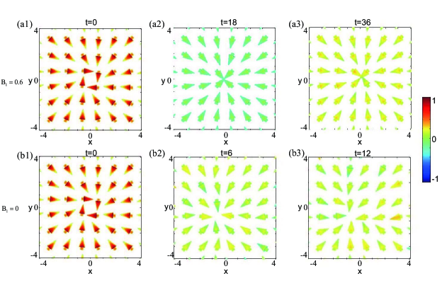
Figure 14: (Color online). (a1)-(a3) Dynamic evolution of the spin texture of the M-PCV in $x$-$y$ plane, where the strength of the magnetic field gradient $B_{1}=0.6$, the weak SO coupling strength $\kappa=2$, the spin-dependent interaction parameter $\lambda_{2}=-75$, spin-independent interaction parameter $\lambda_{0}=7500$, the optical trap frequencies $\omega_{r}=\omega_{z}=2\pi\times 250$Hz, and the real time $t^{\prime}=0.64t$ msec. (a1) $t=0$. (a2) $t=18$. (a3) $t=36$. (b1)-(b3) Dynamic evolution of the spin texture of the M-PCV in $x$-$y$ plane, where the strength of the magnetic field gradient $B_{1}=0$, other parameters are the same as those in (a1) - (a3). (b1) $t=0$. (b2) $t=6$. (b3) $t=12$. The unit of the length is $\sqrt{\hbar/m\omega}$, the unit of the strength of the magnetic field gradient is $\omega\hbar/(g_{F}\mu_{B}a_{h})$, the unit of the SO coupling strength is $\sqrt{\hbar\omega/m}$, and the scale for three dimension system is $34.2\mu m\times 34.2\mu m\times 34.2\mu m$.

The effect of the quadrupole field gradient on the monopoles

Because different external magnetic fields will change the positions of Dirac strings and spin direction, so we investigate the influence of the quadrupole field gradient on the monopoles, where $\kappa=2$, $\lambda_{2}=-75$, $\lambda_{0}=7500$, and $\omega_{r}=\omega_{z}=2\pi\times 250$ Hz. In Figs. 10(a1)-10(a3), when the strength of the quadrupole field gradient is negative, such as $B_{1}=-0.6$, the antimonopoles emerges in the system. The structures of the antimonopoles in terms of every spin components are as follows: a singly anti-vortex line in the $m_{F}=+1$ component, a soliton in the $m_{F}=0$ component, and a singly vortex line in the $m_{F}=-1$ component, where the phenomenon is contrary, comparing with that of the monopoles with $B_{1}=0.6$. In Figs. 10(b1)-10(b3), when $B_{1}$ is the small positive value such as $B_{1}=0.2$, we find that the results in the case of weak quadrupole field gradient are similar to those for $B_{1}=0.6$, which describes a singly vortex line in the $m_{F}=1$ component, a soliton in the $m_{F}=0$ component, and a singly antivortex line in the $m_{F}=-1$ component. In Figs. 10(c1)-10(c3), when $B_{1}$ is the big positive value such as $B_{1}=3.8$, there is a large difference, because the magnetic trap is strongest in $z$ direction. The result shows that the atomic cloud expands from center to both sides in $z$ direction, which is caused that all the atoms are difficult to be bounded in the central region of trap when the strength of the magnetic field gradient increases. A vortex line is terminated in the middle of the atomic cloud for the $m_{F}=+1$ and $m_{F}=-1$ components, and the phase winding of the vortex line is $4\pi$ between the $m_{F}=+1$ and $m_{F}=-1$ component. In addition, for the $m_{F}=0$ component, the vortex line locates in the positive and negative $z$ axis, the corresponding phase winding number of the vortex line is 1.

Ground states for the anisotropic spin-orbit coupling

In Fig. 11, we study the case of the anisotropic SO coupling, where the strength is strong in the $x$ direction with $\kappa_{x}=8$, but is weak in the $y$ direction with $\kappa_{y}=2$. The spin-dependent interaction parameter $\lambda_{2}=-75$ and the strength of the magnetic field gradient $B_{1}=0.6$. The result shows that the monopole vanishes, which is caused that the asymmetric spin-orbit coupling can remove the Dirac string. Instead, the condensate splits into many segments along the $x$ direction, representing a stripe phase along the $x$ direction and a plane wave phase in $y$-$z$ plane. The phases along the $x$ axis are inverse, which is indicated by the black arrows.

Spin textures for the anisotropic spin-orbit coupling

Fig. 12 shows the spin textures of the spinor BECs with the anisotropic SO coupling. For comparison, when the SO coupling is isotropic, such as $\kappa=2$, the spin aligns with the radially inward hedgehog distribution in the $x$-$y$ plane, while the spin textures in the $x$-$z$ and $y$-$z$ planes show the cross hyperbolic distribution [Fig. 12(a)]. When the SO coupling is anisotropic, such as $\kappa_{x}=8$ and $\kappa_{y}=2$, the spin textures show the stripe distribution in the $x$-$y$ and $x$-$z$ planes and the ferromagnetic distribution in the $y$-$z$ plane [Fig. 12(b)]. Furthermore, when the anisotropy of the SO coupling increases, such as $\kappa_{x}=12$ and $\kappa_{y}=2$, we find that the spin textures are similar to those in Fig. 12(b), which suggests that the spin textures are almost not changed when the strength of the anisotropic SO coupling increases [Fig. 12(c)].

The dynamic evolution of the monopoles in the absence of the quadrupole field

In this section, we study the dynamics of the M-PCV when the quadrupole field is turned off. The initial states of the monopoles are shown in Figs. 13(a1)-13(a3). The monopoles are evolved up to $12/\omega$ with a time step $10^{-4}/\omega$. During the time evolution, the isosurface of density becomes rough, see Fig. 13(b1) and Fig. 13(c1). However, the Dirac strings still exist in the condensates, which is denoted by the red arrows in Fig. 13(b2) and Fig. 13(c2). Furthermore, as seen in the phase profile of the wave function, a singly quantized vortex and antivortex do not split, which is denoted by the black circle of arrow and the red circle of arrow, as shown in Fig. 13(b3) and Fig. 13(c3). Compared with the dynamics of the monopoles in the previous work, in which the Dirac strings are observed to expand at about $8/\omega$ 3 . In contrast, in our case, the Dirac strings is not observed to expand until $12/\omega$, which suggests that the SO coupling can protect such the monopole structures during the time evolution in the absence of the external magnetic field.

The dynamic evolution of the spin texture

Fig. 14 is the spin texture of the M-PCV at different times. Figs. 14(a1)-14(a3) indicate the dynamic of the spin texture in the presence of the quadrupole field. We note that the spin texture remains the structure of the south magnetic pole during the time evolution, where the spin aligns with the radially inward hedgehog distribution in the $x$-$y$ plane. Furthermore, when the quadrupole field is turned off, the spin texture of the south magnetic pole remain immobile, see Figs. 14(b1)-14(b3). We further suppose that the M-PCV are stable by means of the dynamic evolution of the spin texture.

References

- (1) V. Pietilä, M. Möttönen, Phys. Rev. Lett. 103, 030401 (2009).
- (2) C. M. Savage, J. Ruostekoski, Phys. Rev. A 68, 034604 (2003).
- (3) E. Ruokokoski, V. Pietilä, M. Möttönen, Phys. Rev. A 84, 063627 (2011).
- (4) C. J. Wang et al., Phys. Rev. Lett. 105, 160403 (2010).
- (5) S. W. Su et al., Phys. Rev. A 86, 023601 (2012).
- (6) C. F. Liu, W. M. Liu, Phys. Rev. A 86, 033602 (2012).
- (7) H. Pu et al., Phys. Rev. A 60, 1463-1470 (1999).
- (8) B. M. Anderson, I. B. Spielman, G. Juzeliūnas, Phys. Rev. Lett. 111, 125301 (2013).
- (9) M. W. Ray et al., Nature 505, 657-660 (2014).
- (10) J. P. A. Devreese, J. Tempere, Carlos A. R. Sá de Melo, Phys. Rev. Lett. 113, 165304 (2014).
- (11) L. F. Chibotaru et al., Nature 408, 833-835 (2000).
- (12) Y. Shin et al., Phys. Rev. Lett. 93, 160406 (2004).
- (13) J. A. M. Huhtamäki et al., Phys. Rev. Lett. 97, 110406 (2006).
- (14) T. Mizushima, K. Machida, T. Kita, Phys. Rev. Lett. 89, 030401 (2002).