Intrinsic strange distributions in the nucleon from the light-cone models

Abstract

Precise knowledge of the strange and antistrange quark distributions of the nucleon is a major step toward better understanding of the strong interaction and the nucleon structure. Moreover, the $s-\bar{s}$ asymmetry in the nucleon plays an important role in some physical processes involving hadrons. The goal of this paper is the study of intrinsic strange contribution to the strange sea of the nucleon. To this aim, we calculate the intrinsic strange distributions from the various light-cone models, including Brodsky, Hoyer, Peterson, and Sakai (BHPS); scalar five-quark and meson-baryon models and then compare their results. These models can lead to the rather different distributions for the intrinsic strange that are dominated in different values of $x$. Furthermore, the meson-baryon model leads to the $s-\bar{s}$ asymmetry that can be comparable in some situations to the result obtained from the global analysis of PDFs. We also present a simple parametrization for each model prediction of intrinsic strange distribution.

I INTRODUCTION

For more than three decades, the intrinsic quark content of the nucleon has been a subject of interest in many studies in hadron physics. The existence of a nonperturbative quark component in the nucleon that is natural in the light-cone Fock space picture was suggested by Brodsky, Hoyer, Peterson, and Sakai (BHPS) Brodsky:1980pb ; 1981 for the first time. According to the BHPS model, there are two distinct types of quark contributions to the nucleon sea: “extrinsic” sea quarks that are produced perturbatively in the splitting of gluons into $q\bar{q}$ pairs in the DGLAP $Q^{2}$ evolution Gribov:1972ri and “intrinsic” sea quarks that are originated through the nonperturbative fluctuations of the nucleon state to five-quark states or a meson plus baryon state. One of the main differences between extrinsic and intrinsic sea quarks is that they have different treatments (“sealike” and valencelike” respectively) and then dominate in different regions of momentum fraction $x$.

One can perhaps divide all of the studies that have been performed so far in the intrinsic quark subject into two main categories: heavy and light intrinsic quarks. Both categories contain theoretical calculations from the various light-cone models, extraction of the probabilities of the intrinsic quarks in the nucleon using available experimental data, and impact of intrinsic quarks on the physical observables sensitive to their distributions. For example, in addition to the BHPS result for the intrinsic charm (IC) distributions in the nucleon, there have been some other theoretical calculations using the scalar five-quark and meson-baryon models performed by Pumplin Pumplin:2005yf and Hobbs et al. Hobbs:2013bia in recent years. In the case of intrinsic light quark distributions, some calculations have been performed by Chang and Pang Chang:2011vx using the BHPS model and there are also a wide range of results from the meson cloud model (MCM) Thomas:1983fh ; Signal:1987gz ; Melnitchouk:1992yd ; Brodsky:1996hc ; Szczurek:1996ur ; Speth:1996pz ; Christiansen:1998dz ; Kumano:1997cy ; Melnitchouk:1998rv ; Cao:1999da ; Cao:2003ny ; Cao:2003zm ; Chen:2009xy ; Traini:2013zqa and chiral quark model (CQM) Manohar:1983md ; Eichten:1991mt ; Szczurek:1996tp ; Song:1997bp ; Wakamatsu:1998rx ; Cheng:1997tt ; Wakamatsu:2003wg ; Wakamatsu:2014asa for either polarized or unpolarized distributions. For the extraction of the probabilities of the intrinsic charm quark in the nucleon, we can point to the analyses performed by BHPS 1981 using diffractive production of charmed hadrons; by Harris et al. Harris:1995jx using the EMC charm production data Aubert:1982tt ; and also some global analyses of parton distribution functions (PDFs) performed so far, including the intrinsic charm contributions in the nucleon Pumplin:2007wg ; Nadolsky:2008zw ; Jimenez-Delgado:2014zga . Moreover, some analyses have been done to extract the probabilities of the light intrinsic quarks Chang:2011vx ; Chang:2011du using the existing $\bar{d}-\bar{u}$ data from the Fermilab E866 Drell-Yan experiment Towell:2001nh and $s+\bar{s}$ data from the HERMES Collaboration measurement of charged kaon production in the semi-inclusive deep inelastic scattering (SIDIS) reaction Airapetian:2008qf . There have also been some studies about the impact of the intrinsic charm quark on processes such as direct photon Bednyakov:2014pqa and $Z$ boson Beauchemin:2014rya production in association with a heavy quark or intrinsic bottom quark on heavy new physics Lyonnet:2015dca at the present hadron colliders such as LHC.

Although the heavy quarks have an important role in the study of many processes in the standard model and beyond it, one of the significant aspects of the nucleon structure is the distribution of strange and antistrange sea quarks and their possible asymmetry. More precise knowledge in this field is very important for better understanding of the nucleon structure and properties of the sea quarks and also for describing processes such as $W$ boson production in association with charm jets Abazov:2014fka or a single top quark production He:2011ss , as well as neutrino interactions Alberico:2001sd ; Dore:2011qe . In the present study, we concentrate on the intrinsic strange quark and calculate its distribution in the nucleon using various light-cone models. Actually, in addition to using the BHPS model as has been done in Ref. Chang:2011vx , we use the scalar five-quark model and a simple meson-baryon model (MBM) introduced by Pumplin Pumplin:2005yf (and applied for the intrinsic charm) to calculate the intrinsic strange distribution in the nucleon numerically and then compare the obtained results with each other. These models can lead to the rather different distributions for the intrinsic strange that can be dominated in different values of $x$. Although the BHPS and scalar five-quark models cannot give us any asymmetry between the $s$ and $\bar{s}$ distributions in the nucleon, the MBM leads to the $s-\bar{s}$ asymmetry. This is a very important conclusion because the perturbative (extrinsic) sea quark distributions in the nucleon are clearly symmetric, so the flavor asymmetry observed in the nucleon strange sea Mason:2007zz certainly has a nonperturbative origin. On the other hand, this asymmetry can also be very important for explaining some experimental results such as the NuTeV anomaly reported by the NuTeV Collaboration Zeller:2001hh . It should be noted that the $s-\bar{s}$ asymmetry can result also from the chiral quark model Wakamatsu:2014asa .

The content of the present paper goes as follows: We describe briefly the light-cone picture of the nucleon and review the BHPS and scalar five-quark models in Sec. II. Then we present and compare the obtained numerical results for the intrinsic strange distribution using these models at the end of this section. A simple meson-baryon model used by Pumplin to calculate the intrinsic charm distributions Pumplin:2005yf is introduced in Sec. III and is used to calculate the intrinsic strange distributions. The calculations are done for two states $K\Lambda$ and $K^{*}\Lambda$ and the resulting $s-\bar{s}$ asymmetry from each of these states, and their sums are also presented. In Sec. IV, we discuss the probability of the intrinsic strange in the nucleon and compare the obtained result for the $s-\bar{s}$ asymmetry from the meson-baryon model presented in Sec. III to the NNPDF Ball:2012cx result for this quantity. We summarize our results and conclusions in Sec. V. A simple parametrization for each model prediction calculated in this work is given in Appendix.

II Five-Quark Models in the light-cone frame

The light-cone frame is very useful to understand the internal structure of hadrons that is one of the most interesting subjects of nuclear and particle physics Brodsky:2004tq . Actually, since in the light-cone Fock space picture the physical vacuum state has a much simpler structure, the light-cone wave functions provide a perfect description of hadrons that is frame and process independent.

In other words, if we define the proton state at fixed light-front time, we find that it is natural to expect nonperturbative intrinsic quark and gluon components in the proton wave function. To be more precise, we cannot consider the proton as a three-quark bound state $|uud\rangle$ and its wave function is a superposition of quark and gluon Fock states such as $|uudg\rangle$, $|uudq\bar{q}\rangle$, etc., or in a more dynamical way provided by the meson-baryon models, a superposition of configurations of off-shell physical particles. As can be seen, one of these states is the five-quark state $|uudq\bar{q}\rangle$. Although one can find a review in Refs. Pumplin:2005yf ; Hobbs:2013bia , in the next two subsections we present briefly two models that can give us $q$ and $\bar{q}$ distributions in the five-quark state $|uudq\bar{q}\rangle$. However, these models cannot give us any information about the magnitude of the probability of this state in the proton and it should be estimated in other ways. We introduce the meson-baryon models in Sec. III separately.

II.1 The BHPS model

The simplest five-quark model is the BHPS model which was proposed in 1980 by Brodsky et al. Brodsky:1980pb . Actually, they found that considering a significant $|uudc\bar{c}\rangle$ Fock component in the proton can lead to enhanced production of charmed hadrons and explain their unexpected large production rates at the forward rapidity region. According to the BHPS model, for a $|uudQ\bar{Q}\rangle$ Fock state of the proton where $Q$ is a heavy quark, neglecting the effect of the transverse momentum in the five-quark transition amplitudes, the momentum distributions of the constituent quarks are given by 1981

$$P(x_{1},...,x_{5})=N\frac{\delta\left(1-\sum\limits_{i=1}^{5}x_{i}\right)}{\left(m_{p}^{2}-\sum\limits_{i=1}^{5}\frac{m_{i}^{2}}{x_{i}}\right)^{2}},$$ (1)

where $m_{p}$ is the mass of the proton and $m_{i}$ and $x_{i}$ are the mass of quark $i$ and momentum fraction carried by it in the five-quark Fock state. The momentum conservation is satisfied by virtue of the delta function. $N$ is the normalization factor and is determined from $\int dx_{1}...\times dx_{5}P(x_{1},...,x_{5})\equiv\mathcal{P}^{Q\bar{Q}}_{5}$, where $\mathcal{P}^{Q\bar{Q}}_{5}$ is the probability of the $|uudQ\bar{Q}\rangle$ Fock state in the proton and expected to be roughly proportional to $1/m_{Q}^{2}$. Integrating Eq. (1) over $x_{1},x_{2},x_{3},$ and $x_{4}$, we get the $\bar{Q}$ distribution in the proton.

In the case of intrinsic charm, BHPS considered another simplifying assumption (in addition to neglecting the effect of the transverse momentum) that the charm mass is much greater than the nucleon and light quark masses [$m_{4}^{2}=m_{5}^{2}\gg m_{p}^{2},m_{i}^{2}(i=1,2,3)$]. In this way, the momentum distribution of $|uudc\bar{c}\rangle$ Fock state becomes

$$P(x_{1},...,x_{5})=N_{5}\frac{x_{4}^{2}x_{5}^{2}}{(x_{4}+x_{5})^{2}}\delta\left(1-\sum_{i=1}^{5}x_{i}\right),$$ (2)

where $N_{5}=N/m_{4,5}^{4}$. Now, this equation can be solved analytically so that by carrying out all of the integrals except one (over $x_{5}$) the $x$ distribution of the intrinsic charm in the proton is obtained as follows

$$P(x_{5}) =\frac{1}{2}N_{5}x_{5}^{2}\Big{[}\frac{1}{3}(1-x_{5})(1+10x_{5}+x_{5}^{2})$$

$$\quad-2x_{5}(1-x_{5})\ln(1/x_{5})\Big{]}.$$ (3)

By performing one more integration over $x_{5}$ we obtain $\mathcal{P}^{c\bar{c}}_{5}=N_{5}/3600$. So far, several studies have been done to estimate the magnitude of $\mathcal{P}^{c\bar{c}}_{5}$ (or momentum fraction carried by intrinsic charm) and have suggested different values for it 1981 ; Harris:1995jx ; Nadolsky:2008zw ; Jimenez-Delgado:2014zga . For a review on the theoretical calculations, constraints from global analyses, and collider observables sensitive to the intrinsic heavy quark distributions, see Ref. Brodsky:2015fna .

As mentioned above, for the case of intrinsic heavy quarks, $\mathcal{P}^{Q\bar{Q}}_{5}$ is proportional to $1/m_{Q}^{2}$. Although this dependence is not applicable for the intrinsic light quarks, we expect that the light five-quark states $|uudu\bar{u}\rangle$, $|uudd\bar{d}\rangle$, and $|uuds\bar{s}\rangle$ have larger probabilities than the $|uudc\bar{c}\rangle$ state in the proton. In recent years, Chang and Pang, generalized the BHPS model to the light five-quark states Chang:2011vx ; Chang:2011du . Actually, in addition to calculating the intrinsic light quark distributions in the proton, they extracted the probabilities of these states ($\mathcal{P}^{q\bar{q}}_{5}$) using available experimental data. Since the main purpose of this work is to calculate the intrinsic strange distribution in the proton from the various light-cone models and to compare them with one another, we also calculate the $x$ distribution of the intrinsic strange quark in the $|uuds\bar{s}\rangle$ Fock state from the BHPS model. We present the obtained results from the five-quark models at the end of this section.

II.2 Scalar five-quark model

Another light-cone model that can be used to extract the $x$ distribution of $Q$ in the $|uudQ\bar{Q}\rangle$ Fock state is the scalar five-quark model. In this model that was presented by Pumplin Pumplin:2005yf during the study of intrinsic heavy quark probability in the proton, the light-cone probability distributions derive directly from Feynman diagram rules and some simplifying assumptions that were considered in the BHPS model are eliminated. According to the scalar five-quark model, if a point scalar particle with mass $m_{0}$ and spin $0$ couples to $N$ scalar particles with masses $m_{1},m_{2},...,m_{N}$ and spin $0$ by a point-coupling $ig$, then the probability distribution $dP$ can be written as

$$dP =\frac{g^{2}}{(16\pi^{2})^{N-1}(N-2)!}\,\prod_{j=1}^{N}dx_{j}\,\delta\left(1-\sum_{j=1}^{N}x_{j}\right)$$

$$\quad\times\int_{s_{0}}^{\infty}ds\,\frac{(s-s_{0})^{N-2}}{(s-m_{0}^{2})^{2}}\,|F(s)|^{2},$$ (4)

where

$$s_{0}=\sum_{j=1}^{N}\frac{m_{j}^{2}}{x_{j}}\,.$$ (5)

Although high mass Fock states are regulated by the factor $(s-m_{0}^{2})^{-2}$ in this model, in order to include the effects of the finite size of the proton we should consider further suppression of high-mass states to make the model more realistic and the integrated probability converge. In this regard, we can include the form factor $F^{2}$ as a function of $s$ that characterizes the dynamics of the bound state to suppress the contributions from the high-mass configurations. Pumplin suggested two exponential and power-law forms for wave function factor $F^{2}$ as follows:

$$|F^{2}(s)|=\exp[-(s-m_{0}^{2})/\Lambda^{2}],$$ (6)

$$|F^{2}(s)|=(s+\Lambda^{2})^{-n},$$ (7)

where $\Lambda$ is a cutoff mass regulator and any value between 2 and 10 GeV can be chosen for it.

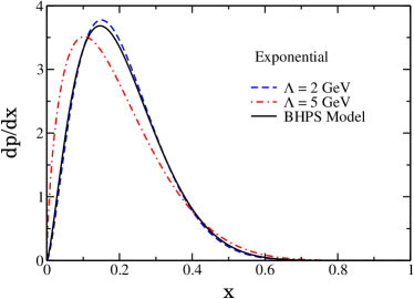
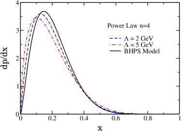
Figure 1: The intrinsic strange distribution from the BHPS and scalar five-quark model with the exponential (top) and power-law (bottom) form factor.

Introducing the BHPS and scalar five-quark models, we can now calculate numerically the intrinsic strange distribution in the proton using these models. Figure 1 (top) shows the strange distribution from the BHPS model [Eq. (1)] using $m_{p}=0.938$, $m_{1}=m_{2}=m_{3}=m_{p}/3$, and $m_{4}=m_{5}=0.5$ in GeV and also the obtained results from the scalar five-quark model [Eq. (II.2)] using the exponential form factor [Eq. (6)] with two values for the parameter $\Lambda$ (2 and 5) and the same values for the physical masses. The strange distribution from the scalar five-quark model and using the power-law form factor with $n=4$ and the mentioned values for the physical masses and parameter $\Lambda$ have been shown in Fig. 1 (bottom) and compared with the BHPS result again. As can be seen from the figures, the obtained results from the BHPS and scalar five-quark model with the exponential form factor and $\Lambda=2$ are very similar, but the result related to the $\Lambda=5$ tended to the lower $x$ and also is smaller and somewhat greater than the BHPS in the regions $x<0.42$ and $x>0.42$, respectively. This latter behavior is also seen when we use the scalar five-quark model with the power-law form factor [Eq. (7)] and $\Lambda=2$ and $5$. It should be noted that we have neglected the probability of the $|uuds\bar{s}\rangle$ state in the proton presently and normalized all curves so that the quark number condition $\int_{0}^{1}dxf(x)=1,(f=s,\bar{s})$ is satisfied.

III Meson-Baryon Model

As mentioned in the previous section, in the light-cone Fock space picture, the nucleon’s wave function can be considered as a superposition of configurations of off-shell physical particles. So one of the phenomenological models for producing intrinsic quark distributions is the meson-cloud or meson-baryon model. Unlike the five-quark models that lead to an equal distribution for strange and antistrange, this more dynamical model can lead to the $s-\bar{s}$ asymmetry in the nucleon sea. Although the original meson-baryon model is rather complicated computationally Hobbs:2013bia ; Melnitchouk:1992yd ; Szczurek:1996ur ; Kumano:1997cy ; Traini:2013zqa , we can consider a simple configuration as has been used in Ref. Pumplin:2005yf . According to the MBM, the nucleon can fluctuate to the virtual meson-baryon Fock states ($N\longrightarrow MB$). For example, in the case of intrinsic strange we can consider the two-body state $K^{+}\Lambda^{0}$, where $K^{+}$ is a $u\bar{s}$ meson and $\Lambda^{0}$ is a $uds$ baryon. To calculate the intrinsic $s$ and $\bar{s}$ distributions in the nucleon, we should model the $K^{+}\Lambda^{0}$ probability distribution, $uds$ distribution in $\Lambda^{0}$, and $u\bar{s}$ distribution in $K^{+}$ and then use the following relation defined as convolutions of the distributions Pumplin:2005yf :

$${{dP}\over{dx}} =\int_{0}^{1}\!dx_{1}\,f_{1}(x_{1})\int_{0}^{1}\!dx_{2}\,f_{2}(x_{2})\,\delta(x-x_{1}x_{2})$$

$$=\int_{x}^{1}{{dy}\over{y}}\,f_{1}(y)\,f_{2}(x/y).$$ (8)

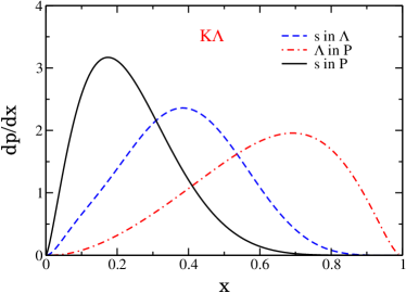
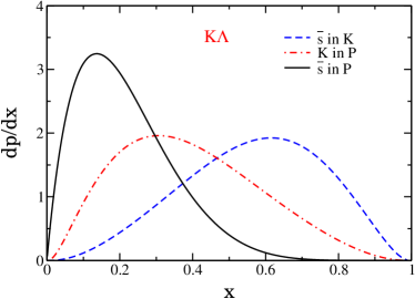
Figure 2: . Momentum distribution of the strange quark in the $\Lambda^{0}$ baryon, $\Lambda^{0}$ from $p\longrightarrow K^{+}\Lambda^{0}$, and final $s$ distribution in the proton (top). Momentum distribution of the antistrange quark in the $K^{+}$ meson, $K^{+}$ from $p\longrightarrow K^{+}\Lambda^{0}$, and final $\bar{s}$ distribution in the proton (bottom).

In this regard, we use Eq. (II.2) with $N=2$ and $F^{2}\varpropto(s_{K\Lambda}+\Lambda^{2}_{p})^{-2}$ and $F^{2}\varpropto(s_{u\bar{s}}+\Lambda^{2}_{K})^{-2}$ to model the $K^{+}\Lambda^{0}$ probability distribution and $u\bar{s}$ distribution in $K^{+}$, respectively. To model the $uds$ distribution in $\Lambda^{0}$ we have $N=3$ and $F^{2}\varpropto(s_{uds}+\Lambda^{2}_{\Lambda})^{-2}$. Moreover, the required physical masses are chosen as $m_{K}=0.4937$, $m_{\Lambda}=1.1157$, $m_{p}=0.938$, $m_{s}=m_{\bar{s}}=0.5$, and $m_{u}=m_{d}=m_{p}/3$ in GeV. Figure 2 shows the obtained results for the $s$ and $\bar{s}$ distributions from $p\longrightarrow K^{+}\Lambda^{0}$ using $\Lambda_{p}=4$ and $\Lambda_{K}=\Lambda_{\Lambda}=2$. As can be seen, the $\bar{s}$ distribution in the $K^{+}$ meson is harder than the $s$ distribution in the $\Lambda^{0}$ baryon. Actually, since the fraction of the hadron mass carried by the constituent quark determines the position of the peak of quark distribution in $x$, this difference is because the $\bar{s}$ carries a larger fraction of the $K^{+}$ mass than the fraction of the $\Lambda^{0}$ mass carried by $s$. Maybe we expect the same behavior for the strange and antistrange distributions in the proton. But in this case the momentum distribution of the meson or baryon in the two-body state $MB$ also has an important rule. We see that by doing the convolution of Eq. (III), the $s$ distribution in the proton is somewhat harder than the $\bar{s}$ distribution.

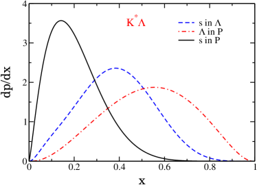
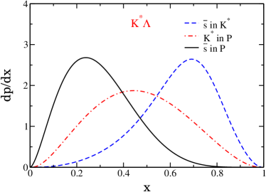
Figure 3: Momentum distribution of the strange quark in the $\Lambda^{0}$ baryon, $\Lambda^{0}$ from $p\longrightarrow K^{*+}\Lambda^{0}$, and final $s$ distribution in the proton (top). Momentum distribution of the antistrange quark in the $K^{*+}$ meson, $K^{*+}$ from $p\longrightarrow K^{*+}\Lambda^{0}$, and final $\bar{s}$ distribution in the proton (bottom).

In addition to the $K^{+}\Lambda^{0}$, we can also consider the following fluctuations:

$$p \longrightarrow K^{0}(d\bar{s})\Sigma^{+}(uus),$$

$$p \longrightarrow K^{+}(u\bar{s})\Sigma^{0}(uds),$$

$$p \longrightarrow K^{*+}(u\bar{s})\Lambda^{0}(uds),$$

$$p \longrightarrow K^{*0}(d\bar{s})\Sigma^{+}(uus),$$

$$p \longrightarrow K^{*+}(u\bar{s})\Sigma^{0}(uds).$$ (9)

But since the physical masses of $K^{0}$ and $K^{+}$, $K^{*0}$ and $K^{*+}$, and even $\Lambda$ and $\Sigma$ are almost equal, the obtained results from some states are the same. Therefore we can consider only two states, $K^{+}\Lambda^{0}$ and $K^{*+}\Lambda^{0}$, that lead to the different shapes for $s$ and $\bar{s}$ distributions and thus the $s-\bar{s}$ asymmetry. We can also sum the results obtained from these states. To calculate $s$ and $\bar{s}$ distributions from $p\longrightarrow K^{*+}\Lambda^{0}$, we use the same physical masses as in the case $K^{+}\Lambda^{0}$, but for the antistrange in $K^{*+}$ we take an effective mass $m_{\bar{s}}=0.7$ to keep $m_{\bar{s}}+m_{u}>m_{K^{*}}$ and avoid mass singularity. Moreover, the $K^{*+}$ mass is taken to be $m_{K^{*}}=0.8917$ GeV. The results for $p\longrightarrow K^{*+}\Lambda^{0}$ are shown in Fig. 3 using $\Lambda_{p}=4$ and $\Lambda_{K^{*}}=\Lambda_{\Lambda}=2$ again. Since we chose a larger mass for the antistrange quark in the $K^{*}$ meson than $K$, the resulting $\bar{s}$ distribution is even harder than before. One can see from Fig. 3 that the momentum distribution of $\Lambda^{0}$ and $K^{*+}$ from $p\longrightarrow K^{*+}\Lambda^{0}$ are peaked almost around $x=0.5$, meaning that the meson and baryon approximately share proton momentum fairly equally. So, because the antistrange quark carries a larger fraction of the total momentum of the meson than the strange quark of the total momentum of the baryon, $\bar{s}$ distribution in the proton is harder and has a greater magnitude than the $s$ distribution at large $x$.

As mentioned above, a main difference between the MBM and five-quark models is that the MBM can lead to the $s-\bar{s}$ asymmetry in the nucleon sea. Actually, since in the MBM framework the probability distributions of the meson and baryon in the proton are different and $s$ and $\bar{s}$ also have different distributions in the baryon and meson respectively, the $s-\bar{s}$ asymmetry is natural. The possibility of this asymmetry in the nucleon was discussed by Signal and Thomas Signal:1987gz by applying MCM for the first time, and after that it has been investigated by other authors Brodsky:1996hc ; Christiansen:1998dz ; Cao:2003ny ; Burkardt:1991di ; Melnitchouk:1999mv . Now, having $s$ and $\bar{s}$ distributions from $p\longrightarrow K^{+}\Lambda^{0}$ and $p\longrightarrow K^{*+}\Lambda^{0}$, we can calculate strange and antistrange asymmetry for each of these states and also their sum in the proton. The results are shown in Fig. 4 and labeled as $K\Lambda$, $K^{*}\Lambda$, and $K\Lambda+K^{*}\Lambda$, respectively. As can be seen, the results from $K^{+}\Lambda^{0}$ and $K^{*+}\Lambda^{0}$ are quite different. The summation of these two states is comparable with full MBM calculations Cao:2003ny .

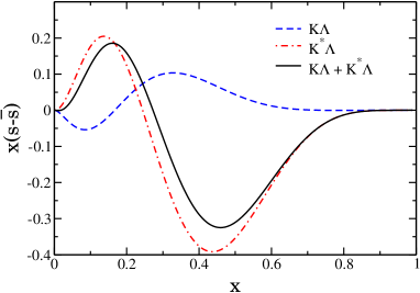
Figure 4: The strange sea asymmetry $x[s(x)-\bar{s}(x)]$ calculated using the meson-baryon model from the fluctuation of the proton to $K\Lambda$ (dashed curve) and $K^{*}\Lambda$ (dotted dashed curve) states and also their summation (solid curve).

IV The probability of intrinsic strange in the nucleon

As mentioned in the introduction, several studies have been done so far to estimate the probability of the intrinsic charm in the nucleon (or momentum fraction carried by intrinsic charm) and have suggested different values for it. For example, BHPS estimate 1 % probability for intrinsic charm in the proton from the diffractive production of charmed hadrons at large longitudinal momentum 1981 . However, few analyses have been done to extract the probabilities of the light intrinsic quarks Chang:2011vx ; Chang:2011du . In order to calculate the probability of the $|uuds\bar{s}\rangle$, Chang and Pang used the existing $x(s+\bar{s})$ data from the HERMES Collaboration measurement of charged kaon production in a SIDIS reaction Airapetian:2008qf . They suggested that these data contain both the extrinsic and intrinsic components of the strange sea that are dominant at small and large $x$, respectively, and also found that data in the $x>0.1$ region can be described well by the intrinsic strange distributions from the BHPS model (see Sec. II.1). They evolved the resulting distributions from the initial scale $\mu=0.3$ GeV and $\mu=0.5$ GeV to $Q^{2}=2.5$ GeV² and then extracted the normalization by fitting data with $x>0.1$, considering the assumption that the extrinsic sea component is negligible in this region. The obtained results for the probability of the $|uuds\bar{s}\rangle$ state are as follows Chang:2011du :

$$\mathcal{P}^{s\bar{s}}_{5} =0.024\qquad(\mu=0.3\ \text{GeV}),$$

$$\mathcal{P}^{s\bar{s}}_{5} =0.029\qquad(\mu=0.5\ \text{GeV}).$$ (10)

As mentioned before, all distributions obtained in the previous sections from the BHPS, scalar five-quark, and meson-baryon models have been normalized to 100 % probability so that the quark number condition $\int_{0}^{1}dxf(x)=1,(f=s,\bar{s})$ is satisfied. At this stage, we can take the above-mentioned probability determined using $\mu=0.5$ and then evolve $s$ and $\bar{s}$ distributions from the MBM (see the previous section) to calculate the $x(s-\bar{s})$ asymmetry at $Q^{2}=16$ GeV², for instance. The evolution of the distributions can be carried out with the QCDNUM package Botje:2010ay . The result is shown in Fig. 5 and also compared with the result of NNPDF2.3 Ball:2012cx for this quantity. As can be seen, the MBM result for $x(s-\bar{s})$ is inside the error bound of the NNPDF2.3 result in some regions of $x$. It highlights this idea in our mind that using the purely theoretical result of the MBM for the $x(s-\bar{s})$ asymmetry can be replaced with a parametrization for this quantity in the global analysis of PDFs.

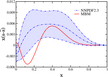
Figure 5: The strange sea asymmetry $x[s(x)-\bar{s}(x)]$ calculated using the meson-baryon model from the fluctuation of the proton to $K\Lambda$ plus $K^{*}\Lambda$ states and evolved from $\mu=0.5$ GeV to $Q^{2}=16$ GeV² (solid line) in comparison with the NNPDF2.3 global fits Ball:2012cx shown by the shaded areas.

V Conclusion

Since Brodsky et al. suggested the possible existence of an intrinsic quark component in the nucleon, the intrinsic quark has been a subject of interest in many studies in hadron physics. These studies can be divided generally into two main categories: heavy and light intrinsic quarks. Although the heavy quarks have an important role in the study of many processes in the standard model and beyond it, one of the significant aspects of the nucleon structure is the distribution of strange and antistrange sea quarks and the possible asymmetry between them. More precise knowledge in this field is very important for better understanding of the nucleon structure and properties of the sea quarks and also for describing processes such as $W$ boson production in association with charm jets Abazov:2014fka or single top quark production He:2011ss , as well as neutrino interactions Alberico:2001sd ; Dore:2011qe . Moreover, the $s-\bar{s}$ asymmetry in the nucleon can also be very important for explaining experimental results such as the NuTeV anomaly reported by the NuTeV Collaboration Zeller:2001hh . In this work, we concentrated on the intrinsic strange quark and calculated its distribution in the nucleon using various light-cone models. Actually, in addition to using the BHPS model Brodsky:1980pb ; 1981 , we used the scalar five-quark model and a simple meson-baryon model introduced by Pumplin Pumplin:2005yf to calculate the intrinsic strange distribution in the nucleon numerically and then compared the results with each other. We found that these models can leads to the rather different distributions for the intrinsic strange that can be dominated in different values of $x$. The resulting distributions from the scalar five-quark model in some situations are very similar to the BHPS result, but in some cases tended to the lower $x$ and also are somewhat greater than the BHPS in larger $x$. Although the BHPS and scalar five-quark models cannot give us any asymmetry between the $s$ and $\bar{s}$ distributions in the nucleon, the MBM leads to the $s-\bar{s}$ asymmetry. This is a very important conclusion because the perturbative (extrinsic) sea quark distributions in the nucleon are clearly symmetric, so the flavor asymmetry in the nucleon certainly has a nonperturbative origin. We compared the obtained result for this asymmetry to the NNPDF2.3 Ball:2012cx result, considering the extracted probability in Ref. Chang:2011du for the intrinsic strange in the nucleon, and found that they are in good agreement with each other. Therefore, maybe using the purely theoretical result of the MBM for the $x(s-\bar{s})$ asymmetry can be replaced with a parametrization for this quantity in the global analysis of PDFs.

Appendix: Parametrization form for the intrinsic strange

We presented various light-cone models for the intrinsic strange in the nucleon and discussed them in detail. As a next work related to the intrinsic strange quark, we provide a simple parametric form for all strange distributions in the nucleon computed in the light-cone framework using the BHPS, scalar five-quark, and MBM models. The parametric form is taken to be

$$f(x) =Ax^{b}(1-x)^{c}.$$ (11)

The normalization constant $A=1/B(1+b,1+c)$, where $B$ is the Euler beta function, obtained from the quark number sum rule $\int_{0}^{1}f(x)dx=1$ and ensure that the distributions are normalized to $1$. The best-fit parameter values are listed in Table 1.

Table 1: Best-fit parameter values for the intrinsic strange.

Model	$a$	$b$	$c$
BHPS	2.265$\times 10^{2}$	8.433	1.449
Exponential ($\Lambda=2$)	3.348$\times 10^{2}$	9.015	1.592
Power law ($\Lambda=2$)	8.514$\times 10^{1}$	7.297	1.053
Exponential ($\Lambda=5$)	3.355$\times 10^{1}$	6.124	0.700
Power law ($\Lambda=5$)	3.028$\times 10^{1}$	5.905	0.673
MBM ($s$ from $K\Lambda$)	1.350$\times 10^{2}$	6.704	1.413
MBM ($\bar{s}$ from $K\Lambda$)	5.549$\times 10^{1}$	6.145	0.973
MBM ($s$ from $K^{*}\Lambda$)	1.404$\times 10^{2}$	7.713	1.277
MBM ($\bar{s}$ from $K^{*}\Lambda$)	1.246$\times 10^{2}$	5.317	1.667

References

- (1) S. J. Brodsky, P. Hoyer, C. Peterson and N. Sakai, Phys. Lett. B 93, 451 (1980).
- (2) S. J. Brodsky, C. Peterson and N. Sakai, Phys. Rev. D 23, 2745 (1981).
- (3) V. N. Gribov and L. N. Lipatov, Sov. J. Nucl. Phys. 15, 438 (1972) [Yad. Fiz. 15, 781 (1972)]; G. Altarelli and G. Parisi, Nucl. Phys. B 126, 298 (1977); Y. L. Dokshitzer, Sov. Phys. JETP 46, 641 (1977) [Zh. Eksp. Teor. Fiz. 73, 1216 (1977)].
- (4) J. Pumplin, Phys. Rev. D 73, 114015 (2006) [hep-ph/0508184].
- (5) T. J. Hobbs, J. T. Londergan and W. Melnitchouk, Phys. Rev. D 89, no. 7, 074008 (2014) [arXiv:1311.1578 [hep-ph]].
- (6) W. C. Chang and J. C. Peng, Phys. Rev. Lett. 106, 252002 (2011) [arXiv:1102.5631 [hep-ph]].
- (7) A. W. Thomas, Phys. Lett. B 126, 97 (1983).
- (8) A. I. Signal and A. W. Thomas, Phys. Lett. B 191, 205 (1987).
- (9) W. Melnitchouk and A. W. Thomas, Phys. Rev. D 47, 3794 (1993).
- (10) S. J. Brodsky and B. Q. Ma, Phys. Lett. B 381, 317 (1996) [hep-ph/9604393].
- (11) A. Szczurek, M. Ericson, H. Holtmann and J. Speth, Nucl. Phys. A 596, 397 (1996) [hep-ph/9602213].
- (12) J. Speth and A. W. Thomas, Adv. Nucl. Phys. 24, 83 (1997).
- (13) H. R. Christiansen and J. Magnin, Phys. Lett. B 445, 8 (1998) [hep-ph/9801283].
- (14) S. Kumano, Phys. Rept. 303, 183 (1998) [hep-ph/9702367].
- (15) W. Melnitchouk, J. Speth and A. W. Thomas, Phys. Rev. D 59, 014033 (1998) [hep-ph/9806255].
- (16) F. G. Cao and A. I. Signal, Phys. Rev. D 60, 074021 (1999) [hep-ph/9907297].
- (17) F. G. Cao and A. I. Signal, Phys. Lett. B 559, 229 (2003) [hep-ph/0302206].
- (18) F. G. Cao and A. I. Signal, Phys. Rev. D 68, 074002 (2003) [hep-ph/0306033].
- (19) H. Chen, F.-G. Cao and A. I. Signal, J. Phys. G 37, 105006 (2010) [arXiv:0912.0351 [hep-ph]].
- (20) M. Traini, Phys. Rev. D 89, no. 3, 034021 (2014) [arXiv:1309.5814 [hep-ph]].
- (21) A. Manohar and H. Georgi, Nucl. Phys. B 234, 189 (1984).
- (22) E. J. Eichten, I. Hinchliffe and C. Quigg, Phys. Rev. D 45, 2269 (1992).
- (23) A. Szczurek, A. J. Buchmann and A. Faessler, J. Phys. G 22, 1741 (1996) [nucl-th/9609042].
- (24) M. Wakamatsu and T. Kubota, Phys. Rev. D 57, 5755 (1998) [hep-ph/9707500]; Phys. Rev. D 60, 034020 (1999) [hep-ph/9809443].
- (25) T. P. Cheng and L. F. Li, Phys. Rev. D 57, 344 (1998) [hep-ph/9701248].
- (26) X. Song, J. S. McCarthy and H. J. Weber, Phys. Rev. D 55, 2624 (1997) [hep-ph/9702363].
- (27) M. Wakamatsu, Phys. Rev. D 67, 034005 (2003).
- (28) M. Wakamatsu, Phys. Rev. D 90, no. 3, 034005 (2014) [arXiv:1405.7095 [hep-ph]].
- (29) B. W. Harris, J. Smith and R. Vogt, Nucl. Phys. B 461, 181 (1996) [hep-ph/9508403].
- (30) J. J. Aubert et al. [European Muon Collaboration], Nucl. Phys. B 213, 31 (1983).
- (31) J. Pumplin, H. L. Lai and W. K. Tung, Phys. Rev. D 75, 054029 (2007) [hep-ph/0701220].
- (32) P. M. Nadolsky, H. L. Lai, Q. H. Cao, J. Huston, J. Pumplin, D. Stump, W. K. Tung and C.-P. Yuan, Phys. Rev. D 78, 013004 (2008) [arXiv:0802.0007 [hep-ph]].; S. Dulat, T. J. Hou, J. Gao, J. Huston, J. Pumplin, C. Schmidt, D. Stump and C.-P. Yuan, Phys. Rev. D 89, no. 7, 073004 (2014) [arXiv:1309.0025 [hep-ph]].
- (33) P. Jimenez-Delgado, T. J. Hobbs, J. T. Londergan and W. Melnitchouk, Phys. Rev. Lett. 114, no. 8, 082002 (2015) [arXiv:1408.1708 [hep-ph]].
- (34) W. C. Chang and J. C. Peng, Phys. Lett. B 704, 197 (2011) [arXiv:1105.2381 [hep-ph]].
- (35) R. S. Towell et al. [NuSea Collaboration], Phys. Rev. D 64, 052002 (2001) [hep-ex/0103030].
- (36) A. Airapetian et al. [HERMES Collaboration], Phys. Lett. B 666, 446 (2008) [arXiv:0803.2993 [hep-ex]].
- (37) V. A. Bednyakov, M. A. Demichev, G. I. Lykasov, T. Stavreva and M. Stockton, Phys. Lett. B 728, 602 (2014).
- (38) P. H. Beauchemin, V. A. Bednyakov, G. I. Lykasov and Y. Y. Stepanenko, Phys. Rev. D 92, no. 3, 034014 (2015) [arXiv:1410.2616 [hep-ph]].
- (39) F. Lyonnet, A. Kusina, T. Ježo, K. Kovarík, F. Olness, I. Schienbein and J. Y. Yu, JHEP 1507, 141 (2015) [arXiv:1504.05156 [hep-ph]].
- (40) V. M. Abazov et al. [D0 Collaboration], Phys. Lett. B 743, 6 (2015) [arXiv:1412.5315 [hep-ex]].
- (41) X. G. He and B. Q. Ma, Eur. Phys. J. A 47, 152 (2011) [arXiv:1104.1894 [hep-ph]].
- (42) W. M. Alberico, S. M. Bilenky and C. Maieron, Phys. Rept. 358, 227 (2002) [hep-ph/0102269].
- (43) U. Dore, Eur. Phys. J. H 37, 115 (2012) [arXiv:1103.4572 [hep-ex]].
- (44) D. Mason et al. [NuTeV Collaboration], Phys. Rev. Lett. 99, 192001 (2007).
- (45) G. P. Zeller et al. [NuTeV Collaboration], Phys. Rev. Lett. 88, 091802 (2002) [Phys. Rev. Lett. 90, 239902 (2003)] [hep-ex/0110059].
- (46) R. D. Ball, V. Bertone, S. Carrazza, C. S. Deans, L. Del Debbio, S. Forte, A. Guffanti and N. P. Hartland et al., Nucl. Phys. B 867, 244 (2013) [arXiv:1207.1303 [hep-ph]].
- (47) S. J. Brodsky, hep-ph/0412101.
- (48) S. J. Brodsky, A. Kusina, F. Lyonnet, I. Schienbein, H. Spiesberger and R. Vogt, Adv. High Energy Phys. 2015, 231547 (2015) [arXiv:1504.06287 [hep-ph]].
- (49) M. Burkardt and B. J. Warr, Phys. Rev. D 45, 958 (1992).
- (50) W. Melnitchouk and M. Malheiro, Phys. Lett. B 451, 224 (1999) [hep-ph/9901321].
- (51) M. Botje, Comput. Phys. Commun. 182, 490 (2011) [arXiv:1005.1481 [hep-ph]].