Abstract

We discuss the limitations of the covariant derivative expansion prescription advocated to compute the one-loop Standard Model (SM) effective lagrangian when the heavy fields couple linearly to the SM. In particular, one-loop contributions resulting from the exchange of both heavy and light fields must be explicitly taken into account through matching because the proposed functional approach alone does not account for them. We review a simple case with a heavy scalar singlet of charge $-1$ to illustrate the argument. As two other examples where this matching is needed and this functional method gives a vanishing result, up to renormalization of the heavy sector parameters, we re-evaluate the one-loop corrections to the T–parameter due to a heavy scalar triplet with vanishing hypercharge coupling to the Brout-Englert-Higgs boson and to a heavy vector-like quark singlet of charged $2/3$ mixing with the top quark, respectively. In all cases we make use of a new code for matching fundamental and effective theories in models with arbitrary heavy field additions.

1 Introduction

The discovery of the Brout-Englert-Higgs (BEH) boson [1] at the LHC [2] has completed the Standard Model (SM), and with it the description of nature with a precision up to few per mille at the electro-weak scale [3]. Moreover, the picture which seems to emerge from the stringent limits set by many of the LHC searches for new physics shows a gap up to the next layer of physics [4] . In this scenario one must use an effective lagrangian approach to study the low energy effects of possible heavy new resonances beyond the LHC reach:

$$\mathcal{L}_{\mathrm{eff}}=\mathcal{L}_{\mathrm{SM}}+\sum_{n>4}\frac{1}{\Lambda^{n-4}}\mathcal{L}_{n}\ ,$$ (1)

where $\mathcal{L}_{\mathrm{SM}}$ is the SM lagrangian, $\Lambda$ the next scale of new physics and $n$ the dimension of the local operators $\mathcal{O}^{(n)}_{i}$ entering in $\mathcal{L}_{n}=\sum_{i}\alpha^{(n)}_{i}\mathcal{O}^{(n)}_{i}$, with $\alpha^{(n)}_{i}$ the corresponding Wilson coefficients. The classification of all operators $\mathcal{O}^{(6)}_{i}$ of dimension 6 in $\mathcal{L}_{6}$ parameterizing the SM extensions in a model independent way was put forward some time ago [6] . The coefficients $\alpha^{(6)}_{i}$, which are expected to gather the largest low-energy contributions of the heavy particles, do depend on the particular SM extension considered. As already noticed, the picture emerging from the LHC searches has boosted the revival of the phenomenological interest in the theoretical prediction of the coefficients of the effective lagrangian up to dimension 6 and up to one-loop order, to cope with the expected experimental precision. With this purpose, the procedure to evaluate the contributions of new (heavy) physics to this order has been revised in Ref. [9] (see [10] for related previous works), providing the one-loop corrections for any SM addition with no linear couplings to the SM (light) fields. In this work the evaluation of the one-loop contribution of a generic heavy sector is reduced to an algebraic problem, getting rid of the difficulties associated to the handling of the loop integrals. This is achieved by the clever use of functional methods using the so called covariant derivative expansion (CDE). Its results readily apply to supersymmetric models with R–parity [11], to models in which the heavy sector does not mix linearly with the SM [12] and, in general, to models with a (discrete) symmetry forbidding such linear terms [13, 14]. This work has been also generalized to extend its range of applicability to the case of non-degenerate heavy field masses [15]. However, as already emphasized, although it has been claimed that the method applies in general, it does not fully account for all quantum corrections when the SM addition involves heavy fields coupling linearly to the light (SM) fields. Since in this case there are one-loop corrections resulting from the exchange of both heavy and light fields within the loops which are not included in the algebraic result, which only accounts for the one-loop diagrams exchanging heavy particles alone . These contributions can be taken care of, however, performing a full matching with the proper local operators, as argued time ago in Ref. [16]. 

Let us be more precise about why this further matching is needed to recover the physical predictions of the original theory. The straightforward application of the CDE results in a different theory in the presence of a heavy sector coupling linearly to the SM. Indeed, the computation of the one-loop effective action ${\cal S}_{\mathrm{eff}}$ for the light (SM) fields $l$ by integrating out a heavy field $h$,

$$e^{\ i{\cal S}_{\mathrm{eff}}[l]}=\int\ {\cal D}h\ e^{\ i{\cal S}[h,l]}\ ,$$ (2)

using the saddle point approximation requires solving the stationary equation for the action ${\cal S}$,

$$\left.\frac{\delta{\cal S}[h,l]}{\delta h}\ \right|_{h=h_{c}}=0\ ,$$ (3)

defining the heavy field classical solution $h_{c}$. Since, it is around this solution that the quantum fluctuations $H=h-h_{c}$ only enter quadratically in the path integral:

$$e^{\ i{\cal S}_{\mathrm{eff}}[l]}= \int\ {\cal D}H\ e^{\ i{\cal S}[h_{c}+H,l]}$$

$$= \int\ {\cal D}He^{\ i\big{(}{\cal S}[h_{c},l]+\frac{1}{2}\left.\frac{\delta^{2}{\cal S}[h,l]}{\delta h^{2}}\ \right|_{h=h_{c}}H^{2}+{\cal O}(H^{3})\big{)}}\ .$$

However, in the presence of linear couplings of the heavy field to the SM fields, ${\cal L}[h,l]\supset h^{\dagger}J[l]+h.c.,$ the equation of motion for $h_{c}$

$$(D^{2}+M^{2}+U[l])\ h_{c}=J[l]+{\cal O}[h_{c}^{2}]\ ,$$ (4)

where $D^{2}=D_{\mu}D^{\mu}$ with $D_{\mu}$ the covariant derivative, $M$ is the $h$ mass and $U$ is the pertinent function of the light fields $l$, is solved by iteration (first equation below) also making use of an asymptotic expansion for the non-local operator ${\cal O}^{-1}=-(D^{2}+M^{2}+U[l])^{-1}$ (second equation)

$$h_{c} \approx\frac{1}{D^{2}+M^{2}+U[l]}J[l]=\frac{1}{M^{2}}\sum_{n=0}^{\infty}\left(-\frac{D^{2}+U[l]}{M^{2}}\right)^{n}J[l]\ .$$ (5)

But, this expansion is only applied for a series solution with a finite number of terms $N$, in which case the linear term is not eliminated but suppressed to the power $M^{-2N}$. In practice, one redefines

$$h=H+\frac{1}{M^{2}}\sum_{n=0}^{N-1}\left(-\frac{D^{2}+U[l]}{M^{2}}\right)^{n}J[l]\approx H+h_{c}\ ,$$ (6)

which is a local, and then allowed, field redefinition. In such a case the linear coupling is only redefined (suppressed) to order $M^{-2N}$,

$${\cal L}[h,l]\supset-H^{\dagger}\left(\frac{D^{2}+U[l]}{M^{2}}\right)^{N}J[l]+h.c.\ ,$$ (7)

and cannot be ignored . One may argue that in the limit $N\rightarrow\infty$ this coupling goes to zero, but then the expansion of ${\cal O}^{-1}$ is asymptotic and the resulting theory and physical predictions of both limits (integrating to arbitrary momenta for $N$ finite and taking $N\rightarrow\infty$ afterwards, or $N\rightarrow\infty$ and integrating to arbitrary momenta) are different. In summary, one can use Eq. (6) keeping track of the linear term suppressed to the corresponding order, or use the quadratic contributions obtained by the CDE with the subsequent matching as indicated in Ref. [16]. We must insist again at this point when using the former approach that although the linear coupling is removed up to order $M^{-2N}$, it contributes to order $M^{-2}$ at one loop, as we will explicitly show in the example below.

In the following section we work out an explicit example, reviewing a simple SM extension studied in full detail in Ref. [18], the addition to the SM of one extra heavy charged scalar singlet $h$ of mass $M\ (=\Lambda)$. We want to elaborate on the fact that the purely functional methods used in the CDE to compute the one-loop effective lagrangian (see Ref. [9]) require further matching, as pointed out in Refs. [16, 18]. The one-loop effective action computed with the proposed functional method is entirely governed by the terms in the full lagrangian which are quadratic in the heavy fields. Furthermore, light fields are kept constant through the calculation. Such contributions correspond, diagrammatically, to one-loop diagrams in which only heavy particles circulate in the loop. In contrast, the diagrammatic calculation of the one-loop effective lagrangian by matching the fundamental and effective theories includes those contributions plus those in which both heavy and light particles circulate in the loop (these diagrams depend on the linear couplings of the heavy fields to the SM). Hence, these latter contributions do have to be taken into account but the CDE with its present formulation does not incorporate them. (See footnote 4.)

As another example of physical interest where further matching is required after using the CDE recipe, we discuss in Section 3 the proper one-loop matching for the T–parameter in two other SM extensions with a heavy sector coupling linearly to the SM. In one case the extended model has an extra heavy scalar triplet coupling linearly to the BEH boson, and in the other one the SM is extended with one extra heavy vector-like quark singlet of charge 2/3 mixing with the top quark. In both cases the CDE alone gives a vanishing one-loop contribution (or gives a contribution that can be reabsorbed in the renormalization of the mass of the heavy fields), in contrast with the straightforward diagrammatic computation. For this calculation we make use of MatchMaker [19], a new automated tool for evaluating tree-level and one-loop matching conditions for arbitrary UV completions into effective lagrangians. The result for the examples worked out below agrees with that obtained in Ref. [20] for the SM unbroken phase in the scalar triplet case, and with the result in Refs. [21, 22] for the vector-like quark singlet addition. Section 4 is devoted to a summary. Technical details on the comparison with previous results in the literature are relegated to an appendix.

2 Extending the SM with a heavy charged scalar singlet

Let us assume the existence of a heavy scalar singlet $h$ of hypercharge $-1$ and of mass $M$, much larger that the electro-weak scale, as in Ref. [18]. Following it, we review in this section the discussion on the need of further matching of the effective field theory (EFT) obtained by the CDE integration of the heavy field with the fundamental theory to one loop, if both must describe the same physics at this order. However, it is not necessary in our case to go through the complete calculation of the one-loop effective lagrangian, which is already worked out in detail in Ref. [18], but it is enough to show that the CDE does not account for a definite physical contribution at this order and hence, that it must be added through matching.

The model we are interested in is described by the lagrangian 

$$\mathcal{L}=\mathcal{L}_{\mathrm{SM}}+\mathcal{L}_{h}=\mathcal{L}_{\mathrm{SM}}+h^{\dagger}\mathcal{O}h+h^{\dagger}J+J^{\dagger}h\ ,$$ (8)

with $\mathcal{O}\equiv-D^{2}-M^{2}-\beta|\phi|^{2}$, and $J\equiv\bar{\tilde{\ell}}_{a}f_{ab}\ell_{b}$. $\phi$ is the SM scalar doublet and $\ell_{a}$ the SM lepton doublet of flavor $a$. Besides, since $\tilde{\ell}=i\tau_{2}\ell^{c}$, $f_{ab}$ is antisymmetric in the flavor indices.

In order to substantiate our point with this example we will identify first a physical amplitude for which the predictions in the fundamental theory and in the EFT obtained applying the CDE prescription are different. This means that the EFT mimicking the fundamental theory must be completed with the required local operators as shown in Ref. [18]. We will then show by analogy that this is needed because the implicit field redefinition used in this case when decomposing the heavy field as its classical counterpart plus its fluctuation corresponds to a non-allowed transformation, for the classical field definition involves a non-local operator which brings it to a different theory. This is made apparent observing that successive heavy field redefinitions in the fundamental theory with local transformations suppressing the linear coupling of the heavy field to SM fields up to order $M^{-2N}$ give the same physical results till the limit $N\rightarrow\infty$ is taken. Then, no linear heavy field coupling to light fields is present at all and the heavy field redefinition involves an infinite sum of terms expanding the non-local operator in Eq. (5), then requiring further matching.

2.1 Matching the EFT to the fundamental theory

As worked out in Ref. [18], the one-loop quantum corrections involving the $\beta$ parameter in Eq. (8) generate the one-loop ($1l$) effective lagrangian (at the renormalization scale $\mu=M$ and omitting flavor indices)

$$\mathcal{L}_{\beta}^{(1l)}=\frac{1}{16\pi^{2}} \Big{\{}M^{2}\beta(1+\Delta)|\phi|^{2}+\frac{\beta^{2}}{2}\Delta|\phi|^{4}$$

$$+\frac{1}{M^{2}}\Big{[}- \frac{\beta^{3}}{6}|\phi|^{6}+\frac{\beta^{2}}{2}(\partial_{\mu}|\phi|^{2})^{2}+\frac{g^{\prime\ 2}\beta}{12}|\phi|^{2}B_{\mu\nu}B^{\mu\nu}\Big{]}$$

$$+\frac{\beta}{M^{2}}\Big{[}|\phi|^{2}(\bar{\ell}f^{\dagger}f\cancel{D}\ell)+\mathrm{h.c.}\Big{]}\Big{\}}\ ,$$ (9)

where dimensional regularization with $d=4-2\epsilon$ is used and $\Delta=1/\epsilon-\gamma_{E}+\ln 4\pi$. $g^{\prime}$ and $B_{\mu\nu}$ stand for the hypercharge coupling and field strength, respectively. The first line in Eq. (9) renormalizes the SM lagrangian while the last two are part of the dimension 6 effective lagrangian. What matters to us, however, is that all the terms but the last one correspond to diagrams with only $h$ running in the loop, whereas the last operator corresponds to a diagram with both heavy ($h$) and light ($\ell$) particles running in the loop. Hence, this latter contribution, which is also proportional to the linear $h$ coupling in the full lagrangian in Eq. (8) (proportional to $f$), is missing in the functional formalism. Therefore, it has to be computed through matching with the fundamental theory. In the effective theory there is no such one-loop contribution to the dimension–6 operator $|\phi|^{2}\bar{\ell}\cancel{D}\ell$. We will then focus on this term.

The matching can be performed by computing the relevant contribution to the $\phi\phi^{\dagger}\to\ell\bar{\ell}$ amplitude, that we denote $\mathrm{i}\mathcal{M}=\bar{u}_{a}(p_{2})\gamma_{\mu}u_{b}(p_{1})\mathrm{i}\mathcal{M}^{\mu}_{ab}$.

Figure 1: Feynman diagram contributing to $\mathrm{i}\mathcal{M}^{\mu}_{ab}$ in the full theory, see Eq. (10).

The result in the fundamental theory reads

$$\mathrm{i}\mathcal{M}_{ab}^{\mu}=-\frac{\mathrm{i}(d-4)(d-2)}{16\pi^{2}d}\frac{\beta(f^{\dagger}f)_{ab}}{M^{4}}(p_{1}^{\mu}+p_{2}^{\mu})A(M^{2})+\dots\ ,$$ (10)

where the relevant Feynman diagram is shown in Fig. 1, the dots denote terms proportional to higher powers of the external momenta. We define the tadpole integral

$$\frac{\mathrm{i}}{16\pi^{2}}A(M^{2})\equiv \mu^{2\epsilon}\int\frac{d^{d}k}{(2\pi)^{d}}\frac{1}{k^{2}-M^{2}+\mathrm{i}\delta}$$

$$= \frac{\mathrm{i}}{16\pi^{2}}M^{2}[\Delta+1-\ln\left(\frac{M^{2}}{\mu^{2}}\right)+\mathcal{O}(\epsilon)]\ ,$$ (11)

where the $\Delta$ term is removed by counterterms in the $\overline{MS}$ scheme. The $d-4$ factor in Eq. (10) guarantees a finite result that reads

$$\mathcal{M}_{ab}^{\mu}=\frac{\beta(f^{\dagger}f)_{ab}}{16\pi^{2}M^{2}}(p_{1}^{\mu}+p_{2}^{\mu})+\dots\ .$$ (12)

There is not such a contribution in the EFT obtained using functional methods and the beyond of the SM tree-level ($0l$) effective lagrangian

$$\mathcal{L}^{(0l)}_{BSM}=-J^{\dagger}\mathcal{O}^{-1}J=\frac{J^{\dagger}J}{M^{2}}+\mathcal{O}(M^{-4})\ .$$ (13)

So both theories are not the same, unless we correct the latter with this additional matching.

Let us now discuss by analogy what happens when we redefine the heavy field in the fundamental theory by successive shifts, Eq. (6), corresponding to keeping only a finite number of terms $N$ in the expansion of ${\cal O}^{-1}$ in Eq. (5). The transformation has unit Jacobian but involves a non-local operator in the limit $N\rightarrow\infty$.

2.2 Heavy field redefinition at leading order

Let us assume $N=1$ in Eq. (6). Then, the heavy field $h$, named $H$ after redefining it, equals to first order

$$h=H+\frac{J}{M^{2}}$$ (14)

and hence, the heavy lagrangian in Eq. (8) reads

$$\mathcal{L}_{H}^{{\rm LO}}=H^{\dagger}\mathcal{O}H+\frac{J^{\dagger}J}{M^{2}}+\frac{1}{M^{2}}\left(H^{\dagger}\hat{\mathcal{O}}J+\mathrm{h.c.}\right)+\frac{J^{\dagger}\hat{\mathcal{O}}J}{M^{4}}\ ,$$ (15)

with

$$\hat{\mathcal{O}}\equiv\mathcal{O}+M^{2}=-D^{2}-\beta|\phi|^{2}\ .$$ (16)

As required, the linear coupling is now suppressed up to order $M^{-2}$. However, this linear coupling, despite its higher-order suppression, still provides the same physical amplitudes, of order $M^{-2}$, because we have only performed an allowed (local) field redefinition. Indeed, focusing again on the amplitude $\phi\phi^{\dagger}\to\ell\bar{\ell}$, the relevant (new) Feynman rules read now

$$\raisebox{-21.33955pt}{\includegraphics[width=42.67912pt]{Htoll}}=\mathrm{i}\frac{p_{H}^{2}}{M^{2}}f^{\dagger}_{ab}\ ,\qquad\raisebox{-21.33955pt}{\includegraphics[width=42.67912pt]{Htollphiphi}}=-\mathrm{i}\frac{\beta}{M^{2}}f^{\dagger}_{ab}\ ,$$ (17)

where the blue dot stands for an order $M^{-2}$ coupling and $p_{H}$ is the $H$ momentum.

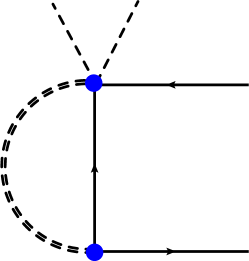
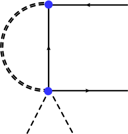
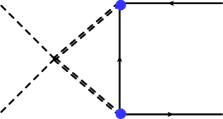
Figure 2: Feynman diagrams contributing to $\mathrm{i}\mathcal{M}^{\mu}_{1}$ (left), $\mathrm{i}\mathcal{M}^{\mu}_{2}$ (center) and $\mathrm{i}\mathcal{M}^{\mu}_{3}$ (right) in Eq. (18) (and Eq. (23) but with the blue dots replaced with red squares).

The three diagrams that contribute to this amplitude are shown in Fig. 2 (we omit flavor indices) with the following result

$$\mathrm{i}\mathcal{M}^{{\rm LO}\,\mu}_{1} =\frac{\mathrm{i}}{16\pi^{2}}\frac{4(d-2)}{d}\frac{\beta(f^{\dagger}f)}{M^{4}}p_{1}^{\mu}A(M^{2})+\dots\ ,$$

$$\mathrm{i}\mathcal{M}^{{\rm LO}\,\mu}_{2} =\frac{\mathrm{i}}{16\pi^{2}}\frac{4(d-2)}{d}\frac{\beta(f^{\dagger}f)}{M^{4}}p_{2}^{\mu}A(M^{2})+\dots\ ,$$

$$\mathrm{i}\mathcal{M}^{{\rm LO}\,\mu}_{3} =-\frac{\mathrm{i}}{16\pi^{2}}(d-2)\frac{\beta(f^{\dagger}f)}{M^{4}}(p_{1}^{\mu}+p_{2}^{\mu})A(M^{2})+\dots\ .$$ (18)

Although each of the three amplitudes is separately divergent, the sum is finite and equals, as expected, Eq. (10):

$$\mathcal{M}^{\mu}=\mathcal{M}^{{\rm LO}\,\mu}_{1}+\mathcal{M}^{{\rm LO}\,\mu}_{2}+\mathcal{M}^{{\rm LO}\,\mu}_{3}\ .$$ (19)

2.3 Heavy field redefinition at next to leading order

Let us repeat the exercise to next order in $M^{-2}$. The heavy field redefinition reads now

$$h=H+\frac{J}{M^{2}}+\frac{\hat{\mathcal{O}}}{M^{4}}J\ ,$$ (20)

which leaves the lagrangian

$$\mathcal{L}_{H}^{{\rm NLO}} =H^{\dagger}\mathcal{O}H+\frac{J^{\dagger}J}{M^{2}}-\frac{1}{M^{4}}\left(H^{\dagger}\hat{\mathcal{O}}^{2}J+\mathrm{h.c.}\right)$$

$$+\frac{J^{\dagger}\hat{\mathcal{O}}J}{M^{4}}+\frac{J^{\dagger}\hat{\mathcal{O}}^{2}J}{M^{6}}+\frac{J^{\dagger}\hat{\mathcal{O}}^{3}J}{M^{8}}\ .$$ (21)

The linear coupling is now suppressed up to order $M^{-4}$. The relevant (new) Feynman rules read at this order

$$=-\mathrm{i}\frac{p_{H}^{4}}{M^{4}}f^{\dagger}_{ab}\ ,$$

$$=\mathrm{i}\frac{\beta}{M^{4}}[p_{H}^{2}+(p_{\ell_{1}}-p_{\ell_{2}})^{2}]f^{\dagger}_{ab}\ ,$$ (22)

where the red square denotes a coupling of order $M^{-4}$ and the fermion momenta, $p_{\ell_{1},\ell_{2}}$ follow the particle flow. The same three diagrams contribute to the $\phi\phi^{\dagger}\to\ell\bar{\ell}$ amplitude but with different couplings and weights (Fig. 2 but with the blue dots replaced with red squares):

$$\mathrm{i}\mathcal{M}^{{\rm NLO}\,\mu}_{1} =\frac{8\mathrm{i}}{16\pi^{2}}\frac{(d-1)p_{1}^{\mu}-p_{2}^{\mu}}{d}\frac{\beta(f^{\dagger}f)}{M^{4}}A(M^{2})+\dots\ ,$$

$$\mathrm{i}\mathcal{M}^{{\rm NLO}\,\mu}_{2} =\frac{8\mathrm{i}}{16\pi^{2}}\frac{(d-1)p_{2}^{\mu}-p_{1}^{\mu}}{d}\frac{\beta(f^{\dagger}f)}{M^{4}}A(M^{2})+\dots\ ,$$

$$\mathrm{i}\mathcal{M}^{{\rm NLO}\,\mu}_{3} =-\frac{\mathrm{i}(d+4)(d-2)}{16\pi^{2}d}\frac{\beta(f^{\dagger}f)}{M^{4}}(p_{1}^{\mu}+p_{2}^{\mu})A(M^{2})+\dots\ .$$ (23)

We find again that the three contributions are separately divergent but their sum is finite and exactly agrees with Eq. (10),

$$\mathcal{M}^{\mu}=\mathcal{M}^{{\rm NLO}\,\mu}_{1}+\mathcal{M}^{{\rm NLO}\,\mu}_{2}+\mathcal{M}^{{\rm NLO}\,\mu}_{3}\ .$$ (24)

As both calculations in the last two subsections show, we recover the physical one-loop amplitude $\phi\phi^{\dagger}\to\ell\bar{\ell}$ to whatever order $M^{-2N}$ we suppress the linear coupling of the heavy field to the SM as long as the heavy field redefinition is allowed (local), i.e. $N<\infty$. But if the $N\rightarrow\infty$ limit is formally taken at the lagrangian level, there is no linear coupling of the heavy field left at all, and we have to deal with a non-local operator (transformation) and a different theory with different physical predictions.

3 SM extensions with heavy scalars and fermions

The issue raised in the previous section also applies to any SM extension with heavy fields coupling linearly to the light fields. In the following we provide the tree-level and one-loop matching conditions relevant for the calculation of the T–parameter [23] in two of these SM extensions. In both cases the one-loop contribution to the T–parameter entirely arises from terms linear in the heavy fields. Hence, these contributions are missing in the one-loop effective lagrangian obtained by functional methods only. 

Using the language of the SM effective lagrangian, the T–parameter, defined as the correction to the SM contribution and absorbing the electro-magnetic coupling constant $\alpha_{EM}=e^{2}/4\pi$ [24], can be written from the Wilson coefficient $\alpha_{1}$ of the dimension-6 effective operator (we omit the superscript indicating the operator dimension in the following)

$$\mathcal{O}_{1}=\left|\phi^{\dagger}D_{\mu}\phi\right|^{2}\quad\mbox{ as }\quad\Delta{\hat{\rm T}}=-\alpha_{1}v^{2},$$ (25)

with $v=174$ GeV the SM vacuum expectation value.

We use MatchMaker [19], an automated tool that performs tree-level and one-loop matching for arbitrary extensions of the SM, for the actual matching. This is performed off-shell, which means that all independent (including redundant) operators with four Higgs bosons and two covariant derivatives have to be considered. In particular, we use the basis

$$\mathcal{O}_{2}=\phi^{\dagger}\phi\ \partial^{2}(\phi^{\dagger}\phi)\ ,\quad\mathcal{R}=\phi^{\dagger}\phi\ \phi^{\dagger}D^{2}\phi\ ,$$ (26)

where the hermitian conjugate of $\mathcal{R}$ has to be also included in the effective lagrangian, with $\alpha_{\mathcal{R}^{\dagger}}=\alpha_{\mathcal{R}}^{\ast}$ . The matching is performed by computing the one-light-particle-irreducible (1LPI) contributions to the Green’s function

$$\langle H_{1}H_{1}^{\ast}H_{2}H_{2}^{\ast}\rangle\ ,\quad{\rm with}\ \phi=\begin{pmatrix}H_{1}\\ H_{2}\end{pmatrix}\ ,$$ (27)

in the full and effective theories. In the effective theory this amplitude reads

$$\mathcal{M}= -\alpha_{1}\big{[}p_{2}\cdot(p_{3}-p_{4})-p_{3}\cdot(p_{3}+p_{4})\big{]}$$

$$+2\alpha_{2}(p_{3}+p_{4})^{2}+\alpha_{\mathcal{R}}^{\ast}\big{[}p_{2}^{2}+p_{4}^{2}\big{]}$$

$$+\alpha_{\mathcal{R}}\big{[}(p_{2}+p_{3})^{2}+(p_{3}+p_{4})^{2}+2p_{2}\cdot p_{4}\big{]},$$ (28)

where all momenta are considered incoming and we have already used momentum conservation to eliminate $p_{1}$. The corresponding calculation in the relevant extension of the SM will fix the matching conditions, up to possible wave function renormalization of the SM fields (see below).

3.1 SM extension with a heavy scalar triplet

In this subsection we consider the first example discussed in Ref. [9]. The same model was previously considered in [20], where the Wilson coefficients were computed by means of matching conditions. The SM addition consists of an extra real scalar in the $(1,3,0)$ representation of the SM gauge symmetry group $SU(3)_{C}\times SU(2)_{L}\times U(1)_{Y}$. Denoting by $\Phi^{a}$ its three $SU(2)_{L}$ components, with $a=1,2,3$, the heavy field lagrangian reads

$$\mathcal{L}_{\Phi} =\frac{1}{2}D_{\mu}\Phi^{a}D^{\mu}\Phi^{a}-\frac{1}{2}M^{2}\Phi^{a}\Phi^{a}-\frac{\lambda_{\Phi}}{4}(\Phi^{a}\Phi^{a})^{2}$$

$$+\kappa\phi^{\dagger}\sigma^{a}\phi\Phi^{a}-\eta\phi^{\dagger}\phi\Phi^{a}\Phi^{a}\ ,$$ (29)

where $\phi$ is the SM scalar doublet with quartic coupling $-\lambda(\phi^{\dagger}\phi)^{2}$ and $\sigma^{a}$ are the Pauli matrices.

The 1LPI contributions to the Green’s function $\langle H_{1}H_{1}^{\ast}H_{2}H_{2}^{\ast}\rangle$ reproduce the momentum structure of the effective theory calculation in Eq. (28) with the tree-level Wilson coefficients

$$\alpha^{(0l)}_{1}=-4\alpha^{(0l)}_{2}=2\alpha^{(0l)}_{\mathcal{R}}=-2\frac{\kappa^{2}}{M^{4}}\ ,$$ (30)

and the one-loop ones

$$\alpha_{1}^{(1l)}= ~{}\frac{\kappa^{2}}{16\pi^{2}M^{4}}\bigg{(}-\frac{\kappa^{2}}{M^{2}}+16\eta-6\lambda-20\lambda_{\Phi}-\frac{5}{4}g_{2}^{2}\bigg{)},$$

$$\alpha_{2}^{(1l)}= ~{}\frac{1}{16\pi^{2}M^{2}}\bigg{[}-\frac{\eta^{2}}{2}-\frac{13}{4}\frac{\kappa^{4}}{M^{4}}$$

$$\qquad-\frac{\kappa^{2}}{M^{2}}\bigg{(}\frac{7}{2}\eta+\frac{15}{16}g_{1}^{2}+\frac{25}{16}g_{2}^{2}-6\lambda-5\lambda_{\Phi}\bigg{)}\bigg{]},$$

$$\alpha_{\mathcal{R}}^{(1l)}= ~{}\frac{\kappa^{2}}{16\pi^{2}M^{4}}\bigg{(}\frac{21}{2}\eta+\frac{5}{8}g_{1}^{2}+\frac{5}{4}g_{2}^{2}-\frac{25}{2}\lambda-10\lambda_{\Phi}+\frac{21}{4}\frac{\kappa^{2}}{M^{2}}\bigg{)}\ .$$ (31)

As mentioned above, the wave function renormalization of the SM fields must be also taken into account. In our case, the heavy triplet also contributes to the SM scalar doublet kinetic term at the loop level:

$$\mathcal{L}_{\mathrm{SM}}=\left(1+\frac{3}{2}\frac{\kappa^{2}}{16\pi^{2}M^{2}}\right)|\partial_{\mu}\phi|^{2}+\ldots\ ,$$ (32)

This term can be reabsorbed by a $\phi$ redefinition

$$\phi\to\left(1-\frac{3}{4}\frac{\kappa^{2}}{16\pi^{2}M^{2}}\right)\phi$$ (33)

which, due to the non-vanishing tree-level contribution to the corresponding effective operators, gives an extra contribution to the one-loop Wilson coefficients. Focusing on $\mathcal{O}_{1}$, we get

$$\alpha_{1}^{(1l)}\to\alpha_{1}^{(1l)}+\frac{6\kappa^{4}}{16\pi^{2}M^{6}}\ .$$ (34)

Thus, our final result for $\alpha_{1}^{(1l)}$ reads

$$\alpha_{1}^{(1l)}=\frac{\kappa^{2}}{16\pi^{2}M^{4}}\left(5\frac{\kappa^{2}}{M^{2}}+16\eta-6\lambda-20\lambda_{\Phi}-\frac{5}{4}g_{2}^{2}\right).$$ (35)

As it is apparent, it is proportional to the linear coupling $\kappa$. In fact, except for the term proportional to $\lambda_{\Phi}$, which arises solely from heavy particles running in the loop and therefore appears in the CDE, all the remaining ones are absent in the functional method calculation alone [9]. This is the result we were looking for. In order to find literal agreement with the calculation in [20] by Khandker, Li and Skiba (KLS), we have to remember that our quartic coupling for the BEH scalar doublet $\lambda=\lambda_{KLS}/4$ and that they use the one-loop renormalized mass for the heavy triplet (as opposed to the tree-level one which we are using). Their relation, which can be found by computing the 1PI contribution to the $\Phi^{a}$ two-point function, is

$$M_{KLS}^{2}=M^{2}\left(1+\frac{2g_{2}^{2}-5\lambda_{\Phi}}{16\pi^{2}}\right),$$ (36)

which in turn gives the extra contribution from $\alpha_{1}^{(0l)}$ to its one-loop counterpart:

$$\alpha_{1}^{(1l)}\to\alpha_{1}^{(1l)}+\frac{(20\lambda_{\Phi}-8g_{2}^{2})\kappa^{2}}{16\pi^{2}M^{4}_{KLS}}\ .$$ (37)

Adding all these contributions (and using the BEH quartic coupling normalization in [20]), we obtain

$$\alpha_{1\ KLS}^{(1l)}=\frac{\kappa^{2}}{16\pi^{2}M_{KLS}^{4}}\bigg{(} 5\frac{\kappa^{2}}{M_{KLS}^{2}}+16\eta-\frac{3}{4}\lambda_{KLS}-\frac{37}{4}g_{2}^{2}\bigg{)},$$ (38)

which coincides with the result obtained in Ref. [20].

3.2 SM extension with a heavy vector-like quark singlet

Our last example is the extension of the SM with a vector-like quark $T$ in the $(3,1,2/3)$ representation of the SM gauge group. In this case the T–parameter is only generated at one-loop order, which was originally computed in [21] (see also [22, 25] for extensions to vector-like quarks in arbitrary representations). The lagrangian involving the heavy field reads

$$\mathcal{L}_{T}=\overline{T}(\mathrm{i}\cancel{D}-M)T-\Big{[}\lambda_{T}~{}\overline{q_{L}}\tilde{\phi}T_{R}+\mathrm{h.c.}\Big{]}\ ,$$ (39)

with $T=T_{L}+T_{R}$, and $L$ and $R$ stand for left- and right-handed fermions, respectively.

The 1LPI calculation of the Green’s function
$\langle H_{1}H_{1}^{\ast}H_{2}H_{2}^{\ast}\rangle$ in the full model has no tree-level contribution but the one-loop values for the Wilson coefficients

$$\alpha_{1}^{(1l)}= ~{}\frac{N_{C}|\lambda_{T}|^{2}}{16\pi^{2}M^{2}}\left(\frac{1}{2}\lambda_{t}^{2}-\frac{1}{2}|\lambda_{T}|^{2}\right),$$

$$\alpha_{2}^{(1l)}= ~{}\frac{N_{C}|\lambda_{T}|^{2}}{16\pi^{2}M^{2}}\left(\frac{3}{2}\lambda_{t}^{2}-\frac{1}{3}|\lambda_{T}|^{2}\right),$$

$$\alpha_{\mathcal{R}}^{(1l)}= ~{}\frac{N_{C}|\lambda_{T}|^{2}}{16\pi^{2}M^{2}}\left(-\frac{1}{2}\lambda_{t}^{2}+\frac{1}{2}|\lambda_{T}|^{2}\right),$$ (40)

where $N_{C}=3$ for a quark and $\lambda_{t}$ is the corresponding top Yukawa coupling (we neglect all other SM Yukawa couplings).

In this case, since the tree-level contribution vanishes, wave function renormalization gives no further contributions at one loop. Previous calculations of the T–parameter in this model have been performed at the electroweak scale. In order to compare with our calculation, we have to run the Wilson coefficients down to the top quark mass and integrate out the top quark with the anomalous couplings induced by the heavy fermion. We present the details of this computation in Appendix A, showing the agreement with previous results.

4 Conclusions

The LHC picture of nature seems to confirm a significant gap between the SM (light fields) and the new layer of physics (heavy fields). This makes the use of EFT compulsory in order to describe (bound) possible small deviations from the SM predictions in the high energy tail of the experimental distributions. Although an EFT with SM symmetries and light fields and arbitrary dimension–6 operators built with them must be in general enough to describe such a scenario (neglecting in this context neutrino masses and the new physics associated to them), it is mandatory to recognize the relations among the different Wilson coefficients of these operators to identify the particular new physics realized in nature. With this purpose, different calculations of the one-loop contributions to the Wilson coefficients of the dimension–6 operators for different SM extensions have been made available using the CDE [9]. SM additions with linear couplings to light fields are treated in the same way as those without them, but in the former case the general results miss extra contributions which must be added by further matching with the specific fundamental theory [16]. Hence, although there are many phenomenologically relevant SM extensions without such linear terms, as supersymmetric theories with unbroken R-parity or models with universal extra dimensions, and in general theories with a discrete symmetry requiring interactions with only an even number of heavy fields, also many phenomenologically relevant theories include heavy fields with linear couplings to the SM, and they demand further treatment.

This problem and its solution were pointed out some time ago [16], and definite examples have been also worked out in detail [18]. The CDE does not include those linear couplings in loops, in contrast with the fundamental theory. What means that the corresponding contributions must be added through matching. (See footnote 4.) In this paper we elaborate on this issue. Noticing first in a simple case with a heavy charged scalar singlet that the problem arises when we perform the non-local heavy field redefinition implicit in this functional treatment of theories with linear couplings of heavy fields to the SM. The fundamental theory (lagrangian) transformed by a local heavy field redefinition expressible as a series with a finite number of terms (local operators) $N$ in general gives the same physical predictions, till the infinite limit $N\rightarrow\infty$ is taken and the series becomes the asymptotic expansion of a non-local operator with a finite radius of convergence. Then, the physical predictions, as well as the resulting theory, are in general different, up to the proper matching.

We have also discussed the beyond the SM contributions to the T–parameter in two other SM extensions with linear couplings of the heavy sector to the light fields, providing the missing pieces in the CDE. They result from the addition of a heavy scalar triplet with vanishing hypercharge and of a heavy vector-like quark of charge 2/3, respectively. As a matter of fact, the CDE gives in both cases a contribution that is either vanishing or can be reabsorbed in the physical definition of the heavy field mass. We obtain perfect agreement with previous calculations in both cases, with Ref. [20] in the scalar triplet case and with Ref. [21] in the vector-like quark one. At any rate, all SM extensions with linear couplings between the heavy and light sectors can require such an extra matching, which can be in general of phenomenological interest (sizable), too.

For our explicit calculations we have made use of the new code MatchMaker [19], aimed at automated calculation of tree-level and one-loop matching conditions in arbitrary extensions of the SM. Details of the code and its use will be presented elsewhere [19].

Appendix A T–parameter at the electroweak scale

In this appendix we show that our result for $\alpha_{1}$ in the SM extension with an extra vector-like quark singlet of hypercharge $2/3$, Eq. (40), agrees with previous calculations of the T–parameter in this model [21]. Previous computations evaluate the T–parameter at the electroweak scale directly in the physical basis (after electroweak symmetry breaking). The exact result, in the limit of large $M$ and only keeping up to $v^{2}/M^{2}$ terms reads [22]

$$\Delta\hat{\rm T}=\frac{N_{C}}{32\pi^{2}}\frac{v^{2}}{M^{2}}\left[|\lambda_{T}|^{4}+2\lambda_{t}^{2}|\lambda_{T}|^{2}\left(\log\frac{M^{2}}{m_{t}^{2}}-1\right)\right],$$ (41)

where $m_{t}$ is the top mass.

In order to reproduce this result in our effective theory approach, using Eq. (25), we need to compute the corresponding Wilson coefficient at the electroweak scale. This involves two steps, first running from the matching scale $M$ down to the top quark mass and second integrating out the top quark with the anomalous couplings that are induced by the heavy quark. These two steps are described in more detail in the next two subsections.

A.1 Running to $\mu=m_{t}$

Given the values of the Wilson coefficients at certain scale, they can be computed at any other energy (provided no new thresholds are crossed) by means of the renormalization group equations (RGE). Since this running is already a loop effect and there are no large logarithms involved, in order to recover the one-loop result in the full theory we just need to include in the running the effective operators that are generated at tree level. In the model at hand we have [26]

$$\mathcal{L}_{6}^{(0l)}=\alpha_{\phi q}^{(1)}\mathcal{O}_{\phi q}^{(1)}+\alpha_{\phi q}^{(3)}\mathcal{O}_{\phi q}^{(3)}+\alpha_{u\phi}\mathcal{O}_{u\phi}+h.c.\ ,$$ (42)

where the operators, following now standard notation, are defined

$$\mathcal{O}_{\phi q}^{(1)} =\mathrm{i}\ \phi^{\dagger}D_{\mu}\phi\ \bar{q}\gamma^{\mu}q\ ,$$

$$\mathcal{O}_{\phi q}^{(3)} =\mathrm{i}\ \phi^{\dagger}\sigma^{a}D_{\mu}\phi\ \bar{q}\gamma^{\mu}\sigma^{a}q\ ,$$

$$\mathcal{O}_{u\phi} =\phi^{\dagger}\phi\ \bar{q}\tilde{\phi}t\ ,$$ (43)

with coefficients

$$\alpha_{\phi q}^{(1)}=-\alpha_{\phi q}^{(3)}=\frac{|\lambda_{T}|^{2}}{4M^{2}},\quad\alpha_{u\phi}=2\lambda_{t}\alpha_{\phi q}^{(1)}\ .$$ (44)

The RGE for $\alpha_{1}$ can be found in [27], where it is named $\alpha_{\phi D}$, (see also [28] for further calculations relevant for the RGE of the SM EFT) and reads

$$16\pi^{2}\frac{\mathrm{d}\ \alpha_{1}}{\mathrm{d}\log\mu}=8N_{C}\lambda_{t}^{2}\alpha_{\phi q}^{(1)}+\ldots\ ,$$ (45)

where we have only included the contribution proportional to operators generated at tree level and proportional to the top Yukawa coupling. In the leading-log approximation we obtain

$$\alpha_{1}(m_{t})= ~{}\alpha_{1}(M)-\frac{N_{C}\lambda_{t}^{2}\alpha_{\phi q}^{(1)}(M)}{2\pi^{2}}\log\left(\frac{M}{m_{t}}\right)$$

$$= ~{}\frac{N_{C}}{32\pi^{2}M^{2}}\bigg{[}\lambda_{t}^{2}|\lambda_{T}|^{2}-|\lambda_{T}|^{4}-2\lambda_{t}^{2}|\lambda_{T}|^{2}\log\left(\frac{M^{2}}{m_{t}^{2}}\right)\bigg{]}.$$ (46)

Using Eq. (25), we already recognize the terms proportional to $|\lambda_{T}|^{4}$ and $\lambda_{t}^{2}|\lambda_{T}|^{2}\log(M^{2}/m_{t}^{2})$ in Eq. (41). The term proportional to $\lambda_{t}^{2}|\lambda_{T}|^{2}$ is not quite right yet but that is just because we are still missing the second step: integrating out the top quark.

A.2 Matching at $\mu=m_{t}$

In this last step we have to integrate out the top quark. At this point we have to go to the broken phase of the SM. However, we can still neglect the bottom mass in our calculation if we want to reproduce Eq. (41). Thus, in the new effective theory with the top quark integrated out, the relevant fields are massless and the one-loop calculation in the effective theory side gives vanishing results. Thus we only need to perform the computation in the full theory, i.e. in the SM. However, due to the terms in $\mathcal{L}_{6}^{(0l)}$ the top couplings are modified by terms of order $v^{2}/M^{2}$ and these have to be taken into account. In particular, the $W_{3}t_{L}t_{L}$ and $W_{1}t_{L}b_{L}$ couplings are modified [26] (note that in this reference $v=246$ GeV is used and therefore, there is a relative factor $\sqrt{2}$ between the corresponding expressions there and here):

$$g_{W_{3}t_{L}t_{L}} =g_{W_{3}t_{L}t_{L}}^{\mathrm{SM}}[1-2v^{2}(\alpha_{\phi q}^{(1)}-\alpha_{\phi q}^{(3)})]$$

$$=g_{W_{3}t_{L}t_{L}}^{\mathrm{SM}}\left(1-\frac{|\lambda_{T}|^{2}v^{2}}{M^{2}}\right),$$

$$g_{W_{1}t_{L}b_{L}} =g_{W_{1}t_{L}b_{L}}^{\mathrm{SM}}[1+2v^{2}\alpha_{\phi q}^{(3)}]$$

$$=g_{W_{1}t_{L}b_{L}}^{\mathrm{SM}}\left(1-\frac{|\lambda_{T}|^{2}v^{2}}{2M^{2}}\right).$$ (47)

Then, the top contribution to $\hat{{\rm T}}$ in the presence of these anomalous couplings writes (see Ref. [25], noting that $\hat{{\rm T}}={\rm T}\ \alpha_{EM}$)

$$\hat{{\rm T}}(m_{t}^{+})= \frac{N_{C}}{32\pi^{2}v^{2}}\Bigg{\{}\bigg{|}\frac{g_{W_{1}t_{L}b_{L}}}{g^{\mathrm{SM}}_{W_{1}t_{L}b_{L}}}\bigg{|}^{2}\theta_{+}(m_{t},m_{b})$$

$$-\frac{1}{2}\bigg{[}\bigg{|}\frac{g_{W_{3}t_{L}t_{L}}}{g^{\mathrm{SM}}_{W_{3}t_{L}t_{L}}}\bigg{|}^{2}\theta_{+}(m_{t},m_{t})+\theta_{+}(m_{b},m_{b})\bigg{]}\Bigg{\}},$$ (48)

where $m_{t}^{\pm}\equiv\lim_{x\to 0}m_{t}\pm x$ and

$$\theta_{+}(y_{1},y_{2}) \equiv y_{1}^{2}+y_{2}^{2}-\frac{2y_{1}^{2}y_{2}^{2}}{y_{1}^{2}-y_{2}^{2}}\log\frac{y_{1}^{2}}{y_{2}^{2}}$$

$$-2\left(y_{1}^{2}\log\frac{y_{1}^{2}}{\mu^{2}}+y_{2}^{2}\log\frac{y_{2}^{2}}{\mu^{2}}\right)+\frac{y_{1}^{2}+y_{2}^{2}}{2}\Delta\ .$$

We temporarily keep the bottom mass to regulate IR divergencies. Using the explicit values for the anomalous couplings in Eq. (47) and taking the bottom mass to zero we get

$$\hat{{\rm T}}(m_{t}^{+}) =\frac{N_{C}}{32\pi^{2}v^{2}}\bigg{\{}\bigg{(}1-\frac{|\lambda_{T}|^{2}v^{2}}{M^{2}}\bigg{)}\theta_{+}(m_{t},0)$$

$$\qquad-\frac{1}{2}\bigg{(}1-\frac{2|\lambda_{T}|^{2}v^{2}}{M^{2}}\bigg{)}\theta_{+}(m_{t},m_{t})\bigg{\}}$$

$$=\frac{N_{C}}{32\pi^{2}}\lambda_{t}^{2}\left(1-\frac{|\lambda_{T}|^{2}v^{2}}{M^{2}}\right)=\hat{\rm T}_{\mathrm{SM}}+\Delta\hat{\rm T}(m_{t}^{+})\ ,$$ (49)

where we have explicitly split the result into the SM contribution, $\hat{{\rm T}}_{\rm SM}$, and a correction, $\Delta\hat{{\rm T}}(m_{t}^{+})$, which is proportional to $|\lambda_{T}|^{2}$. We have used that

$$\theta_{+}(m,0)=m^{2}[1-2\log(m^{2}/\mu^{2})+\Delta/2],$$

and

$$\theta_{+}(m,m)=m^{2}[-4\log(m^{2}/\mu^{2})+\Delta],$$

and set $\mu=m_{t}$ to eliminate the logarithms. We have only kept terms up to $\mathcal{O}(v^{2}/M^{2})$ and used the $\overline{\rm MS}$ renormalization scheme to remove the divergent term left, proportional to $\Delta$ and $|\lambda_{T}|^{2}$, with the corresponding counterterm.

Since the contribution below $m_{t}$ vanishes if we neglect the bottom mass, we have ended the calculation. Putting all pieces together:

$$\Delta\hat{{\rm T}}(m_{t}^{-}) =-v^{2}\alpha_{\phi D}(m_{t})+\Delta\hat{{\rm T}}(m_{t}^{+})$$

$$=\frac{N_{C}}{32\pi^{2}}\frac{v^{2}}{M^{2}}\left[|\lambda_{T}|^{4}+2\lambda_{t}^{2}|\lambda_{T}|^{2}\left(\log\frac{M^{2}}{m_{t}^{2}}-\frac{1}{2}\right)\right]-\frac{N_{C}}{32\pi^{2}}\frac{v^{2}}{M^{2}}\lambda_{t}^{2}|\lambda_{T}|^{2}$$

$$=\frac{N_{C}}{32\pi^{2}}\frac{v^{2}}{M^{2}}\left[|\lambda_{T}|^{4}+2\lambda_{t}^{2}|\lambda_{T}|^{2}\left(\log\frac{M^{2}}{m_{t}^{2}}-1\right)\right],$$ (50)

which is exactly Eq. (41).

References

- [1] F. Englert and R. Brout, Phys. Rev. Lett. 13 (1964) 321; P. W. Higgs, Phys. Rev. Lett. 13 (1964) 508.
- [2] G. Aad et al. [ATLAS Collaboration], Phys. Lett. B 716 (2012) 1 [arXiv:1207.7214 [hep-ex]]; S. Chatrchyan et al. [CMS Collaboration], Phys. Lett. B 716 (2012) 30 [arXiv:1207.7235 [hep-ex]].
- [3] F. del Aguila and J. de Blas, Fortsch. Phys. 59 (2011) 1036 [arXiv:1105.6103 [hep-ph]]; J. de Blas, M. Chala and J. Santiago, Phys. Rev. D 88 (2013) 095011 [arXiv:1307.5068 [hep-ph]]; J. de Blas, EPJ Web Conf. 60 (2013) 19008 [arXiv:1307.6173 [hep-ph]]; A. Pomarol and F. Riva, JHEP 1401 (2014) 151 [arXiv:1308.2803 [hep-ph]]; M. Ciuchini, E. Franco, S. Mishima, M. Pierini, L. Reina and L. Silvestrini, arXiv:1410.6940 [hep-ph]; A. Falkowski and F. Riva, JHEP 1502 (2015) 039 [arXiv:1411.0669 [hep-ph]]; A. Buckley, C. Englert, J. Ferrando, D. J. Miller, L. Moore, M. Russell and C. D. White, Phys. Rev. D 92 (2015) 9, 091501 [arXiv:1506.08845 [hep-ph]]; arXiv:1512.03360 [hep-ph]; J. de Blas, M. Chala and J. Santiago, JHEP 1509 (2015) 189 [arXiv:1507.00757 [hep-ph]]; A. Falkowski, M. Gonzalez-Alonso, A. Greljo and D. Marzocca, Phys. Rev. Lett. 116 (2016) 1, 011801 [arXiv:1508.00581 [hep-ph]]; L. Berthier and M. Trott, arXiv:1508.05060 [hep-ph].
-
[4]
https://twiki.cern.ch/twiki/bin/view/AtlasPublic
/ExoticsPublicResults
https://twiki.cern.ch/twiki/bin/view/CMSPublic
/PhysicsResultsEXO - [5] The ATLAS collaboration, ATLAS-CONF-2015-081; CMS Collaboration [CMS Collaboration], CMS-PAS-EXO-15-004.
- [6] W. Buchmuller and D. Wyler, Nucl. Phys. B 268 (1986) 621.
- [7] S. Weinberg, Phys. Rev. Lett. 43 (1979) 1566.
- [8] H. Georgi, Nucl. Phys. B 361 (1991) 339; Nucl. Phys. B 363, 301 (1991); C. Arzt, Phys. Lett. B 342 (1995) 189 [hep-ph/9304230]; G. F. Giudice, C. Grojean, A. Pomarol and R. Rattazzi, JHEP 0706 (2007) 045 [hep-ph/0703164]; J. A. Aguilar-Saavedra, Nucl. Phys. B 812 (2009) 181 [arXiv:0811.3842 [hep-ph]]; Nucl. Phys. B 821 (2009) 215 [arXiv:0904.2387 [hep-ph]]; B. Grzadkowski, M. Iskrzynski, M. Misiak and J. Rosiek, JHEP 1010 (2010) 085 [arXiv:1008.4884 [hep-ph]].
- [9] B. Henning, X. Lu and H. Murayama, JHEP 1601 (2016) 023 [arXiv:1412.1837 [hep-ph]].
- [10] M. K. Gaillard, Nucl. Phys. B 268 (1986) 669; O. Cheyette, Nucl. Phys. B 297 (1988) 183.
- [11] J. Fan, M. Reece and L. T. Wang, JHEP 1508 (2015) 152 [arXiv:1412.3107 [hep-ph]]; A. Drozd, J. Ellis, J. Quevillon and T. You, JHEP 1506 (2015) 028 [arXiv:1504.02409 [hep-ph]]; R. Huo, arXiv:1509.05942 [hep-ph]; J. Brehmer, A. Freitas, D. Lopez-Val and T. Plehn, arXiv:1510.03443 [hep-ph].
- [12] R. Huo, JHEP 1509 (2015) 037 [arXiv:1506.00840 [hep-ph]].
- [13] T. Appelquist, H. C. Cheng and B. A. Dobrescu, Phys. Rev. D 64 (2001) 035002 [hep-ph/0012100].
- [14] H. C. Cheng and I. Low, JHEP 0309 (2003) 051 [hep-ph/0308199].
- [15] A. Drozd, J. Ellis, J. Quevillon and T. You, arXiv:1512.03003 [hep-ph].
- [16] E. Witten, Nucl. Phys. B 104 (1976) 445; Nucl. Phys. B 122 (1977) 109.
- [17] J. Leon, J. Perez-Mercader and M. F. Sanchez, Phys. Lett. B 208 (1988) 463; C. k. Lee, T. Lee and H. Min, Phys. Rev. D 39 (1989) 1681.
- [18] M. S. Bilenky and A. Santamaria, Nucl. Phys. B 420 (1994) 47 [hep-ph/9310302]; In *Wendisch-Rietz 1994, Proceedings, Theory of elementary particles* 215-224 [hep-ph/9503257].
- [19] C. Anastasiou, A. Lazopoulos and J. Santiago, in preparation.
- [20] Z. U. Khandker, D. Li and W. Skiba, Phys. Rev. D 86 (2012) 015006 [arXiv:1201.4383 [hep-ph]]; see also W. Skiba, arXiv:1006.2142 [hep-ph].
- [21] L. Lavoura and J. P. Silva, Phys. Rev. D 47 (1993) 2046.
- [22] M. Carena, E. Ponton, J. Santiago and C. E. M. Wagner, Nucl. Phys. B 759 (2006) 202 [hep-ph/0607106].
- [23] M. E. Peskin and T. Takeuchi, Phys. Rev. D 46 (1992) 381.
- [24] R. Barbieri, A. Pomarol, R. Rattazzi and A. Strumia, Nucl. Phys. B 703 (2004) 127 [hep-ph/0405040].
- [25] C. Anastasiou, E. Furlan and J. Santiago, Phys. Rev. D 79 (2009) 075003 [arXiv:0901.2117 [hep-ph]].
- [26] F. del Aguila, M. Perez-Victoria and J. Santiago, JHEP 0009 (2000) 011 [hep-ph/0007316].
- [27] E. E. Jenkins, A. V. Manohar and M. Trott, JHEP 1401 (2014) 035 [arXiv:1310.4838 [hep-ph]].
- [28] J. Elias-Miro, J. R. Espinosa, E. Masso and A. Pomarol, JHEP 1311 (2013) 066 [arXiv:1308.1879 [hep-ph]]; E. E. Jenkins, A. V. Manohar and M. Trott, JHEP 1310 (2013) 087 [arXiv:1308.2627 [hep-ph]]; R. Alonso, E. E. Jenkins, A. V. Manohar and M. Trott, JHEP 1404 (2014) 159 [arXiv:1312.2014 [hep-ph]].