DESY 16-020 ISSN 0418-9833
January 2016

Counting master integrals: Integration by parts vs. functional equations

Abstract

We illustrate the usefulness of functional equations in establishing relationships between master integrals under the integration-by-parts reduction procedure by considering a certain two-loop propagator-type diagram as an example.

An adequate theoretical interpretation of the increasingly precise data collected by the experiments at the CERN Large Hadron Collider and elsewhere necessitates advanced technologies for the calculation of radiative corrections, which typically depend on several different mass scales. Feynman diagrams involving quantum loops may be reduced to so-called master integrals via dedicated algorithms, such as integration by parts (IBP) [1, 2]. The evaluation of the master integrals often turns out to be a bottleneck of the entire theoretical analysis, the more if many different mass scales are involved. Any method to reduce the number of master integrals of a given set of Feynman diagrams is, therefore, highly welcome. Recently, relationships between master integrals of the two-loop sunset diagram were found in Refs. [3, 4]. In the present paper, a new relationship of this type will be presented, which is found using functional equations [5].

The derivation of functional equations for integrals with two and more loops is much more complicated than in the one-loop case. In this following, we consider two-loop propagator-type integrals. Two-loop integrals differ by the number of internal lines. According to the algorithm of Refs. [5, 6], functional equations may be obtained from recurrence relations connecting two-loop integrals with different numbers of lines. The most complicated integrals in such a functional equation may be eliminated by an appropriate choice of four-momenta and masses.

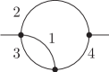
Figure 1: Two-loop diagram corresponding to integral $V^{(d)}_{1111}$.

Let us consider the following two-loop propagator-type integral with four internal lines:

$$V^{(d)}_{\nu_{1}\nu_{2}\nu_{3}\nu_{4}}(m_{1}^{2},m_{2}^{2},m_{3}^{2},m_{4}^{2};q^{2})=\frac{1}{\left(i\pi^{d/2}\right)^{2}}$$ (1)

$${}\times\int\int\frac{d^{d}k_{1}d^{d}k_{2}}{[(k_{1}-k_{2})^{2}-m_{1}^{2}]^{\nu_{1}}[k_{2}^{2}-m_{2}^{2}]^{\nu_{2}}[(k_{1}-q)^{2}-m_{3}^{2}]^{\nu_{3}}[(k_{2}-q)^{2}-m_{4}^{2}]^{\nu_{4}}},$$

where $d$ is the space-time dimension. The Feynman diagram corresponding to this integral is shown in Fig. 1. With the aid of generalized recurrence relations given in Ref. [7], the integral $V^{(d)}_{\nu_{1}\nu_{2}\nu_{3}\nu_{4}}$ with arbitrary integers $\nu_{j}$ may be reduced to the integral $V^{(d)}_{1111}$, four two-loop integrals with three lines of the type

$$J^{(d)}_{\nu_{1}\nu_{2}\nu_{3}}(m_{1}^{2},m_{2}^{2},m_{3}^{2};q^{2})$$ (2)

$$= \frac{1}{\left(i\pi^{d/2}\right)^{2}}\int\int\frac{d^{d}k_{1}d^{d}k_{2}}{[k_{1}^{2}-m_{1}^{2}]^{\nu_{1}}[(k_{1}-k_{2})^{2}-m_{2}^{2}]^{\nu_{2}}[(k_{2}-q)^{2}-m_{3}^{2}]^{\nu_{3}}},$$

the product of a one-loop propagator-type integral,

$$I_{2}^{(d)}(m_{1}^{2},m_{2}^{2};q^{2})=\frac{1}{i\pi^{d/2}}\int\frac{d^{d}k_{1}}{(k_{1}^{2}-m_{1}^{2})[(k_{1}-q)^{2}-m_{2}^{2}]},$$ (3)

with masses $m_{2}^{2}$ and $m_{3}^{2}$, times a one-loop vacuum-type integral,

$$T_{a}(m_{1}^{2})=\frac{1}{i\pi^{d/2}}\int\frac{d^{d}k_{1}}{k_{1}^{2}-m_{1}^{2}},$$ (4)

and products of one-loop vacuum-type integrals with different masses.

In Ref. [7], several generalized recurrence relations for the integral $V^{(d)}_{\nu_{1}\nu_{2}\nu_{3}\nu_{4}}$ were presented. One of these relations, namely the one in Eq. (55) therein, reads:

$$m_{4}^{2}V^{(d)}_{1112} = \frac{(d-3)u_{624}u_{246}\Delta_{134}+(d-3)u_{314}u_{134}\Delta_{246}+(d-4)\Delta_{134}\Delta_{246}}{2\Delta_{134}\Delta_{246}}$$ (5)

$${}\times V^{(d)}_{1111}+\frac{u_{624}\Delta_{134}-u_{314}\Delta_{246}}{\Delta_{134}\Delta_{246}}m_{3}^{2}J^{(d)}_{112}(m_{1}^{2},m_{2}^{2},m_{3}^{2};q^{2})$$

$${}+\frac{u_{624}\Delta_{134}-u_{134}\Delta_{246}}{\Delta_{134}\Delta_{246}}m_{1}^{2}J^{(d)}_{211}(m_{1}^{2},m_{2}^{2},m_{3}^{2};q^{2})$$

$${}+\frac{2m_{2}^{2}(q^{2}-m_{2}^{2})}{\Delta_{246}}J^{(d)}_{121}(m_{1}^{2},m_{2}^{2},m_{3}^{2},q^{2})$$

$${}-\frac{u_{624}(3d-8)}{2\Delta_{246}}J^{(d)}_{111}(m_{1}^{2},m_{2}^{2},m_{3}^{2};q^{2})$$

$${}+\frac{(d-2)u_{624}}{2\Delta_{246}}J_{111}(m_{1}^{2},m_{3}^{2},m_{4}^{2};0)$$

$${}+\frac{(d-2)}{2\Delta_{134}}\left[u_{314}T^{(d)}_{1}(m_{3}^{2})+u_{134}T^{(d)}_{1}(m_{1}^{2})\right]I_{2}^{(d)}(m_{2}^{2},m_{4}^{2};q^{2}).$$

where $u_{ijk}=m_{i}^{2}-m_{j}^{2}-m_{k}^{2}$ and $\Delta_{ijk}=-u_{ijk}(u_{jik}+u_{kij})-u_{jik}u_{kij}$. According to the algorithm of Ref. [5] to obtain functional equation, one has to eliminate from Eq. (5) the integrals $V_{1111}^{(d)}$ and $V_{1112}^{(d)}$ by an appropriate choice of four-momentum and masses. For $m_{4}=0$, the left-hand side of Eq. (5) vanishes, so that we obtain an expression for the integral $V_{1111}^{(d)}$ in terms of integrals with lesser numbers of lines, namely,

$$V_{1111}^{(d)} = \frac{2m_{1}^{2}(q^{2}+u_{312})}{(d-2)(m_{3}^{2}-m_{1}^{2})(q^{2}-m_{2}^{2})}J_{211}(m_{1}^{2},m_{2}^{2},m_{3}^{2};q^{2})$$ (6)

$${}-\frac{2m_{3}^{2}(q^{2}+u_{123})}{(d-2)(m_{3}^{2}-m_{1}^{2})(q^{2}-m_{2}^{2})}J_{112}(m_{1}^{2},m_{2}^{2},m_{3}^{2};q^{2})$$

$${}+\frac{4m_{2}^{2}}{(d-2)(q^{2}-m_{2}^{2})}J_{121}(m_{1}^{2},m_{2}^{2},m_{3}^{2};q^{2})$$

$${}-\frac{(3d-8)}{(d-2)(q^{2}-m_{2}^{2})}J_{111}(m_{1}^{2},m_{2}^{2},m_{3}^{2};q^{2})$$

$${}+\frac{1}{q^{2}-m_{2}^{2}}J_{111}(m_{1}^{2},m_{3}^{2},0;0)$$

$${}+\frac{1}{m_{1}^{2}-m_{3}^{2}}\left[T^{(d)}_{1}(m_{1}^{2})-T^{(d)}_{1}(m_{3}^{2})\right]I_{2}^{(d)}(m_{2}^{2},0;q^{2}).$$

After multiplying Eq. (6) with the factor $q^{2}-m_{2}^{2}$ and then setting $q^{2}=m_{2}^{2}$, the contribution proportional to the integral $V^{(d)}_{1111}$ drops out, and obtain the following relationship:

$$0 = 2m_{1}^{2}J^{(d)}_{211}(m_{1}^{2},m_{2}^{2},m_{3}^{2};m_{2}^{2})+4m_{2}^{2}J^{(d)}_{121}(m_{1}^{2},m_{2}^{2},m_{3}^{2};m_{2}^{2})$$ (7)

$${}+2m_{3}^{2}J^{(d)}_{112}(m_{1}^{2},m_{2}^{2},m_{3}^{2};m_{2}^{2})-(3d-8)J^{(d)}_{111}(m_{1}^{2},m_{2}^{2},m_{3}^{2};m_{2}^{2})$$

$${}+(d-2)J_{111}^{(d)}(m_{1}^{2},m_{3}^{2},0;0).$$

Equation (7) connects two-loop propagator-type integrals with different kinematics. The analytic expression for the integral $J_{111}^{(d)}(m_{1}^{2},m_{2}^{2},m_{3}^{2};0)$ in terms of the Gauss hypergeometric function ${}_{2}F_{1}$ presented in Ref. [8] is considerably simpler than the analytic expressions for the integrals $J_{111}^{(d)}$ and $J_{211}^{(d)}$ with external momentum square being different from zero. It is interesting to notice that the Cayley–Menger determinant

$$D_{123} = [q^{2}-(m_{1}+m_{2}+m_{3})^{2}][q^{2}-(m_{1}-m_{2}+m_{3})^{2}]$$ (8)

$${}\times[q^{2}-(m_{1}+m_{2}-m_{3})^{2}][q^{2}-(m_{1}-m_{2}-m_{3})^{2}]$$

for this kinematics is different from zero:

$$\left.D_{123}\right|_{q^{2}=m_{2}^{2}}=(m_{1}^{2}-m_{3}^{2})^{2}[(m_{1}^{2}-m_{3}^{2})^{2}+8m_{2}^{2}(2m_{2}^{2}-m_{1}^{2}-m_{3}^{2})].$$ (9)

Thus, Eq. (7) is a clear illustration that the number of nontrivial basis integrals, as predicted by IBP, may re reduced not only if $D_{123}=0$ or one mass is zero as was observed in Ref. [7], but also for other values of four-momentum momentum square and masses. One possible interpretation is that the total number of basis integrals arising from the IBP reduction of the integral $J^{(d)}_{\nu_{1}\nu_{2}\nu_{3}}(m_{1}^{2},m_{2}^{2},m_{3}^{2};m_{2}^{2})$ with arbitrary integer powers of propagators remains the same, but that one nontrivial integral may be replaced by simpler one.

For the particular case when $m_{1}=0$ and $m_{2}^{2}=m_{3}^{2}=m^{2}$, the reduction of the number of basis integrals was observed in Ref. [9]. For this kinematics, Eq. (7) yields

$$J^{(d)}_{211}(m^{2},0,m^{2};m^{2})=\frac{3d-8}{6m^{2}}J^{(d)}_{111}(m^{2},0,m^{2};m^{2})-\frac{d-2}{6m^{2}}J_{111}^{(d)}(m^{2},0,0;0),$$ (10)

so that, instead of two nontrivial integrals, only one nontrivial basis integral,$J^{(d)}_{111}(m^{2},0,m^{2};m^{2})$, remains.

Putting $m_{3}=0$ in Eq. (7), we recover Eq. (9) in Ref. [3], which was obtained there as a special case via differential reduction [10, 11, 12, 13, 14, 15, 16, 17, 18, 19, 20, 21, 22]. Another generalization of Eq. (9) in Ref. [3] was obtained in Ref. [4] using IBP in connection with an effective propagator mass [23].

We would like mention that Eq. (7) connects integrals of different mass assignments. Such integrals may arise from rather different Feynman diagrams. Relationships of this type may be very useful, e.g., for proving the gauge independence of radiative corrections to physical observables.

In conclusion, functional equations [5, 6] provide a powerful tool for disclosing hidden relationships between what appear to be master integrals upon standard applications of the IBP reduction procedure [1, 2]. Similar relationships have previously been revealed using differential reduction [3] and a nonstandard variant of the IBP reduction procedure implemented with propagator masses to be integrated over [4].

References

• [1] F. Tkachov, A theorem on analytical calculability of 4-loop renormalization group functions, Phys.Lett. B100 (1981) 65–68. doi:10.1016/0370-2693(81)90288-4.
• [2] K. Chetyrkin, F. Tkachov, Integration by parts: The algorithm to calculate $\beta$-functions in 4 loops, Nucl.Phys. B192 (1981) 159–204. doi:10.1016/0550-3213(81)90199-1.
• [3] M. Yu. Kalmykov, B. A. Kniehl, Counting master integrals: Integration by parts vs. differential reduction, Phys. Lett. B702 (2011) 268–271. arXiv:1105.5319, doi:10.1016/j.physletb.2011.06.094.
• [4] B. A. Kniehl, A. V. Kotikov, Counting master integrals: Integration-by-parts procedure with effective mass, Phys. Lett. B712 (2012) 233–234. arXiv:1202.2242, doi:10.1016/j.physletb.2012.04.071.
• [5] O. Tarasov, New relationships between Feynman integrals, Phys.Lett. B670 (2008) 67–72. arXiv:0809.3028, doi:10.1016/j.physletb.2008.10.021.
• [6] O. Tarasov, Functional equations for Feynman integrals, Phys.Part.Nucl.Lett. 8 (2011) 419–427. doi:10.1134/S1547477111050219.
• [7] O. Tarasov, Generalized recurrence relations for two-loop propagator integrals with arbitrary masses, Nucl.Phys. B502 (1997) 455–482. arXiv:hep-ph/9703319, doi:10.1016/S0550-3213(97)00376-3.
• [8] A. Davydychev, J. Tausk, Two-loop self-energy diagrams with different masses and the momentum expansion, Nucl.Phys. B397 (1993) 123–142. doi:10.1016/0550-3213(93)90338-P.
• [9] A. Davydychev, M. Kalmykov, New results for the $\epsilon$-expansion of certain one-, two- and three-loop Feynman diagrams, Nucl.Phys. B605 (2001) 266–318. arXiv:hep-th/0012189, doi:10.1016/S0550-3213(01)00095-5.
• [10] M. Yu. Kalmykov, Gauss hypergeometric function: reduction, $\epsilon$-expansion for integer/half-integer parameters and Feynman diagrams, JHEP 04 (2006) 056. arXiv:hep-th/0602028, doi:10.1088/1126-6708/2006/04/056.
• [11] M. Kalmykov, V. V. Bytev, B. A. Kniehl, B. F. L. Ward, S. A. Yost, Feynman Diagrams, Differential Reduction, and Hypergeometric Functions, PoS ACAT08 (2008) 125. arXiv:0901.4716.
• [12] V. V. Bytev, M. Kalmykov, B. A. Kniehl, B. F. L. Ward, S. A. Yost, Differential Reduction Algorithms for Hypergeometric Functions Applied to Feynman Diagram Calculation, arXiv:0902.1352.
• [13] V. V. Bytev, M. Yu. Kalmykov, B. A. Kniehl, Differential reduction of generalized hypergeometric functions from Feynman diagrams: One-variable case, Nucl. Phys. B836 (2010) 129–170. arXiv:0904.0214, doi:10.1016/j.nuclphysb.2010.03.025.
• [14] M. Yu. Kalmykov, B. A. Kniehl, All-order $\epsilon$ expansions of hypergeometric functions of one variable, Phys. Part. Nucl. 41 (2010) 942–945. arXiv:1003.1965, doi:10.1134/S1063779610060250.
• [15] M. Yu. Kalmykov, B. A. Kniehl, “Sixth root of unity” and Feynman diagrams: hypergeometric function approach point of view, Nucl. Phys. B (Proc. Suppl.) 205-206 (2010) 129–134. arXiv:1007.2373, doi:10.1016/j.nuclphysbps.2010.08.031.
• [16] S. A. Yost, V. V. Bytev, M. Yu. Kalmykov, B. A. Kniehl, B. F. L. Ward, Differential Reduction Techniques for the Evaluation of Feynman Diagrams, PoS ICHEP2010 (2010) 135. arXiv:1101.2348.
• [17] V. V. Bytev, M. Yu. Kalmykov, B. A. Kniehl, HYPERDIRE, HYPERgeometric functions DIfferential REduction: MATHEMATICA-based packages for differential reduction of generalized hypergeometric functions ${}_{p}F_{p-1}$, $F_{1}$, $F_{2}$, $F_{3}$, $F_{4}$, Comput. Phys. Commun. 184 (2013) 2332–2342. arXiv:1105.3565, doi:10.1016/j.cpc.2013.05.009.
• [18] S. A. Yost, V. V. Bytev, M. Yu. Kalmykov, B. A. Kniehl, B. F. L. Ward, The Epsilon Expansion of Feynman Diagrams via Hypergeometric Functions and Differential Reduction, arXiv:1110.0210.
• [19] M. Yu. Kalmykov, B. A. Kniehl, Mellin–Barnes representations of Feynman diagrams, linear systems of differential equations, and polynomial solutions, Phys. Lett. B714 (2012) 103–109. arXiv:1205.1697, doi:10.1016/j.physletb.2012.06.045.
• [20] V. V. Bytev, M. Kalmykov, B. A. Kniehl, When epsilon-expansion of hypergeometric functions is expressible in terms of multiple polylogarithms: the two-variables examples, PoS LL2012 (2012) 029. arXiv:1212.4719.
• [21] V. V. Bytev, M. Yu. Kalmykov, S.-O. Moch, HYPERgeometric functions DIfferential REduction (HYPERDIRE): MATHEMATICA based packages for differential reduction of generalized hypergeometric functions: $F_{D}$ and $F_{S}$ Horn-type hypergeometric functions of three variables, Comput. Phys. Commun. 185 (2014) 3041–3058. arXiv:1312.5777, doi:10.1016/j.cpc.2014.07.014.
• [22] V. V. Bytev, B. A. Kniehl, HYPERDIRE HYPERgeometric functions DIfferential REduction: Mathematica-based packages for the differential reduction of generalized hypergeometric functions: Horn-type hypergeometric functions of two variables, Comput. Phys. Commun. 189 (2014) 128–154. arXiv:1309.2806, doi:10.1016/j.cpc.2014.11.022.
• [23] B. A. Kniehl, A. V. Kotikov, Calculating four-loop tadpoles with one non-zero mass, Phys.Lett. B638 (2006) 531–537. arXiv:hep-ph/0508238, doi:10.1016/j.physletb.2006.04.057.