Proving the existence of numerically detected planar limit cycles

Abstract.

This paper deals with the problem of location and existence of limit cycles for real planar polynomial differential systems. We provide a method to construct Poincaré–Bendixson regions by using transversal curves, that enables us to prove the existence of a limit cycle that has been numerically detected. We apply our results to several known systems, like the Brusselator one or some Liénard systems, to prove the existence of the limit cycles and to locate them very precisely in the phase space. Our method, combined with some other classical tools can be applied to obtain sharp bounds for the bifurcation values of a saddle-node bifurcation of limit cycles, as we do for the Rychkov system.

1. Introduction

We consider real planar polynomial differential systems of the form

(1) $$\dot{x}=dx/dt=P(x,y),\quad\dot{y}=dy/dt=Q(x,y),$$

where $P(x,y)$ and $Q(x,y)$ are real polynomials. We denote by $X=(P,Q)$ the vector field associated to (1) and $z=(x,y)$. So, (1) can be written as $\dot{z}=X(z).$

When dealing with system (1) one of the main problems is to determine the number and location of its limit cycles. Recall that a limit cycle is an isolated periodic orbit of the system. For a given vector field, when it is not very near of a bifurcation, the limit cycles can usually be detected by numerical methods. A bifurcation is a qualitative change in the behaviour of a vector field as a parameter of the system is varied. This phenomenon can involve a change in the stability of a limit cycle or the creation or destruction of one or more limit cycles. If a periodic orbit is stable (unstable), then forward (backward) numerical integration of a trajectory with an initial condition in its basin of attraction will converge to the periodic orbit as $t\to\infty$ ($t\to-\infty$). Once for a given vector field a limit cycle is numerically detected there is no general method to rigourously prove its existence. In this work we present a procedure to prove the existence of a limit cycle in that situation. The method is based on the Poincaré–Bendixson theorem, see for instance [5, 12] and also Theorem 1. Poincaré–Bendixson theorem (cf. Theorem 1) can be very useful to prove the existence of a limit cycle and to give a region where it is located. However, this result is hardly found in applications due to the difficulty of constructing the boundaries of a Poincaré–Bendixson region. Our aim in this work is to give a constructive procedure for finding transversal curves which define Poincaré–Bendixson regions and thus, to prove the existence of limit cycles that have been numerically detected.

Consider a smooth and non-empty curve $C$ in $\mathbb{R}^{2}$. Let $C=\{z(s)=(x(s),y(s))\,:\,s\in\mathcal{I}\}$ be a class $\mathcal{C}^{1}$ parametrization of $C$, where $\mathcal{I}$ is a real interval. It is said that $C$ is regular if $z^{\prime}(s)\neq(0,0)$ for all $s\in\mathcal{I}$. Given $z=(x,y)$ we set $z^{\perp}=(y,-x)$ and $(x_{1},y_{1})\cdot(x_{2},y_{2})=x_{1}x_{2}+y_{1}y_{2}$. A contact point with the flow given by (1) is a point $z(s)$ such that the tangent vector to $C$ at this point, $z^{\prime}(s)$ is parallel to $X(z(s)).$

As usual, we will say that a curve $C$ is transversal with respect to the flow given by (1) if the scalar product

$$X(z(s))\cdot(z^{\prime}(s))^{\perp}=P\left(z(s)\right)y^{\prime}(s)-Q\left(z(s)\right)x^{\prime}(s)$$

does not change sign and vanishes only on finitely many contact points. When the above scalar product does not vanish we will say that the curve is strictly transversal. Notice that intuitively, these definitions mean that the flow of system (1) “crosses $C$ in the same direction” on all its points.

A $\mathcal{C}^{1}$ closed plane curve $C$ is a regular parameterized curve $z:[a,b]\longrightarrow\mathbb{R}^{2}$ such that $z$ and its derivative coincide at $a$ and $b$. The curve is said to be simple if it has no self-intersections, that is if $s_{1},s_{2}\in[a,b)$ and $s_{1}\neq s_{2}$, then $z(s_{1})\neq z(s_{2})$. For further information about these classical concepts, see for instance [4].

A transversal section of system (1) is an arc of a curve without contact points. Given a limit cycle $\Gamma$ there always exist a transversal section $\Sigma$ which can be parameterized by $r\in(-\rho,\rho)$ with $\rho>0$ and $r=0$ corresponding to a common point between $\Gamma$ and $\Sigma$. Given $r\in(-\rho,\rho)$, we consider the flow of system (1) with initial point the one corresponding to $r$ and we follow this flow for positive values of $t$. It can be shown, see for instance [12], that for $\rho$ small enough, the flow cuts $\Sigma$ again at some point corresponding to the parameter $\mathcal{P}(r)$. The map $r\longrightarrow\mathcal{P}(r)$ is called the Poincaré map associated to the limit cycle $\Gamma$ of system (1). It is clear that $\mathcal{P}(0)=0$. If $\mathcal{P}^{\prime}(0)\neq 1$, the limit cycle $\Gamma$ is said to be hyperbolic. If the expansion of $\mathcal{P}(r)$ around $r=0$ is of the form $\mathcal{P}(r)=r+a_{\mu}r^{\mu}+\mathcal{O}(r^{\mu+1})$ with $a_{\mu}\neq 0$ and $\mu\geq 2$, we say that $\Gamma$ is a multiple limit cycle of multiplicity $\mu$. A classical result, see for instance [12], states that if $\Gamma=\left\{\gamma(t):t\in[0,T)\right\}$, where $\gamma(t)$ is the parametrization of the limit cycle in the time variable $t$ of system (1) and $T>0$ is the period of $\Gamma$, that is, the lowest positive value for which $\gamma(0)=\gamma(T)$, and $\gamma(0)=\Gamma\cap\Sigma$, then

$$\mathcal{P}^{\prime}(0)=\exp\left\{\int_{0}^{T}\operatorname{div}X\left(\gamma(t)\right)dt\right\},$$

where

$$\operatorname{div}X(x,y)=\frac{\partial P}{\partial x}(x,y)+\frac{\partial Q}{\partial y}(x,y)$$

is the divergence of $X$. Hence

$$k:=\int_{0}^{T}\operatorname{div}X\left(\gamma(t)\right)dt\neq 0$$

is the condition for a limit cycle $\Gamma$ to be hyperbolic. It is clear that if $k>0$ (resp. $k<0$), then $\Gamma$ is an unstable (resp. stable) limit cycle. If $\Gamma$ is a multiple limit cycle of multiplicity $\mu$ and $\mu$ is odd, then $\Gamma$ is unstable if $a_{\mu}>0$ and stable if $a_{\mu}<0$. If $\mu$ is even, then the limit cycle $\Gamma$ is said to be semi-stable. For the definitions and related results, see for instance [5, 12, 17].

The Poincaré–Bendixson theorem, which can be found for instance in [5, Sec. 1.7] or in [12, Sec. 3.7], has as a corollary the following result which motivates the definition of Poincaré–Bendixson region. See also Theorem 4.7 of [18, Chap. 1].

Theorem 1.

[Poincaré-Bendixson annular Criterion] Suppose that $R$ is a finite region of the plane $\mathbb{R}^{2}$ lying between two $\mathcal{C}^{1}$ simple disjoint closed curves $C_{1}$ and $C_{2}$. If

• the curves $C_{1}$ and $C_{2}$ are transversal for system (1) and the flow crosses them towards the interior of $R$, and

• $R$ contains no critical points.

Then, system (1) has an odd number of limit cycles (counted with multiplicity) lying inside $R$.

In such a case, we say that $R$ is a Poincaré–Bendixson annular region for system (1).

As we have already stated our aim is to find transversal curves which define Poincaré–Bendixson annular regions and thus, to prove the existence of limit cycles, as well as to locate them. In the paper [6] we dealt with the same problem and we described a way to provide transversal conics which give rise to a Poincaré–Bendixson annular region. In this previous paper we treated several examples for which we numerically knew the existence of a limit cycle, but we did not use this information. Besides, we could not ensure the existence of the transversal conics. In the present work we give an answer to the following question: if one numerically knows the existence of a hyperbolic limit cycle, can one analytically prove the existence of such limit cycle? In section 3 we describe a method which answers this question in an affirmative way.

The following theorem is the main result of this paper and it gives the theoretical basis of the method described in section 3. We prove:

Theorem 2.

Let $\Gamma=\{(\gamma(t)\,:\,t\in[0,T]\}$ be a $T$-periodic hyperbolic limit cycle of (1), parameterized by the time $t$. Define

$$\tilde{z}_{\varepsilon}(t)=\gamma(t)+\varepsilon\tilde{u}(t)(\gamma^{\prime}(t))^{\perp},$$

where

(2) $$\tilde{u}(t)=\frac{1}{||\gamma^{\prime}(t)||^{2}}\exp\left\{\int_{0}^{t}\operatorname{div}X\left(\gamma(s)\right)\,ds-\kappa\,t\right\}$$

and $\kappa=\frac{k}{T}=\frac{1}{T}\int_{0}^{T}\operatorname{div}X(\gamma(t))\,dt.$ Then, the curve $\left\{\tilde{z}_{\varepsilon}(t)\,:\,t\in[0,T]\right\}$ is $T$-periodic and, for $|\varepsilon|>0$ small enough, it is strictly transversal to the flow associated to system (1).

The proof of this result is given in section 2. Note that in its statement $\tilde{u}(t)>0$ for all $t$ and $\kappa\neq 0$ because $\Gamma$ is hyperbolic.

Notice that as a consequence of the above result, the curve $\tilde{z}_{\varepsilon}(t)$ is a transversal oval close to the limit cycle $\Gamma$ for $|\varepsilon|>0$ small enough, which is inside or outside it depending on the sign of $\varepsilon$.

As an illustration of the effectiveness of our approach we apply it to locate the limit cycles in two celebrated planar differential systems, the van der Pol oscillator and the Brusselator system, see sections 4.1 and 4.2, respectively. As we will see, the van der Pol limit cycle is “easier” to be treated than the one of the Brusselator system. In section 4.3 we give an explanation for the different level of difficulty for studying both limit cycles. We prove that the different level of difficulty is hidden in the sizes of the respective Fourier coefficients of the two limit cycles, see Theorem 6. This theorem also shows that our approach for detecting strictly transversal closed curves always works in finitely many steps.

Finally, to show the applicability of the method to detect bifurcation values, we use it to find a sharp interval for the bifurcation value for a saddle-node bifurcation of limit cycles for the Rychkov system. Recall that a saddle-node bifurcation of limit cycles occurs when a stable limit cycle and an unstable limit cycle coalesce and become a double semi-stable limit cycle. A saddle-node bifurcation of limit cycles corresponds to an elementary catastrophe of fold type.

In 1975 Rychkov([13]) proved that the system

$$\dot{x}\,=\,y-\left(x^{5}-\mu x^{3}+\delta x\right),\quad\dot{y}\,=\,-x,$$

with $\delta,\mu\in\mathbb{R},$ has at most 2 limit cycles. Moreover, it is known that it has 2 limit cycles if and only if $\delta>0$ and $0<\delta<\Delta(\mu),$ for some unknown function $\Delta.$ For the value $\delta=\Delta(\mu)$ the system has a double limit cycle and, varying $\delta$, it presents a saddle-node bifurcation of limit cycles. This system is also studied by Alsholm([1]) and Odani([10]). In particular Odani proved that $\Delta(\mu)>{\mu^{2}}/5.$

We believe that it is an interesting challenge to develop methods for finding sharp estimations of $\Delta(\mu)$. Here we will fix our attention on $\delta^{*}:=\Delta(1).$ Notice that Odani’s result implies that $\delta^{*}>1/5=0.2.$ We prove:

Theorem 3.

Let $\delta=\delta^{*}$ be the value for which the Rychkov system

(3) $$\dot{x}\,=\,y-\left(x^{5}-x^{3}+\delta x\right),\quad\dot{y}\,=\,-x$$

has a semi-stable limit cycle. Then $0.224\,{<}\,\delta^{*}\,{<}\,0.2249654.$

The lower bound for $\delta^{*}$ is proved by using the tools introduced in this work. The upper bound is proved by constructing a polynomial function in $(x,y)$ of very high degree such that its total derivative with respect to the vector field does not change sign. This method is proposed and already developed for general classical Liénard systems by Cherkas([2]) and also by Giacomini-Neukirch ([7, 8]).

2. Proof of Theorem 2 and a corollary

Proof of Theorem 2.

To prove that the curve $\tilde{z}_{\varepsilon}(t)$ is $T$-periodic simply notice that $\gamma(t)$ is $T$-periodic and that the function $\tilde{u}(t)$ is $T$-periodic as well, due to its definition (2), because for any real integrable $T$-periodic function $h$, the new function

$$H(t)=\int_{0}^{t}h(s)\,ds-\frac{t}{T}\int_{0}^{T}h(s)\,ds$$

is also $T$-periodic.

Now, we show that the curve $\tilde{z}_{\varepsilon}(t)$, for $|\varepsilon|>0$ small enough, is strictly transversal to system (1). This follows once we prove that

(4) $$X(\tilde{z}_{\varepsilon}(t))\cdot(\tilde{z}_{\varepsilon}^{\prime}(t))^{\perp}=\kappa\mathcal{E}(t)\,\varepsilon+\mathcal{O}(\varepsilon^{2}),$$

where we have introduced, to simplify notation,

$$\mathcal{E}(t):=\exp\left\{\int_{0}^{t}\operatorname{div}X\left(\gamma(s)\right)\,ds-\kappa\,t\right\}>0.$$

Let us prove (4). We drop the dependence on $t$ to simplify notation. Since $\tilde{z}_{\varepsilon}=\gamma+\varepsilon\tilde{u}\gamma^{\prime\perp},$ we have that $\tilde{z}_{\varepsilon}^{\perp}=\gamma^{\perp}-\varepsilon\tilde{u}\gamma^{\prime}$. Then

$$X(\tilde{z}_{\varepsilon}) =X(\gamma+\varepsilon\tilde{u}\gamma^{\prime\perp})=X(\gamma)+\varepsilon\tilde{u}DX(\gamma)\gamma^{\prime\perp}+\mathcal{O}(\varepsilon^{2})$$

$$=\gamma^{\prime}+\varepsilon\tilde{u}DX(\gamma)\gamma^{\prime\perp}+\mathcal{O}(\varepsilon^{2}),$$

$$\tilde{z}_{\varepsilon}^{\prime\perp} =\gamma^{\prime\perp}-\varepsilon\tilde{u}^{\prime}\gamma^{\prime}-\varepsilon\tilde{u}\gamma^{\prime\prime}.$$

Hence $X(\tilde{z}_{\varepsilon})\cdot\tilde{z}_{\varepsilon}^{\prime\perp}=\gamma^{\prime}\cdot\gamma^{\prime\perp}+\tau\varepsilon+\mathcal{O}(\varepsilon^{2})=\tau\varepsilon+\mathcal{O}(\varepsilon^{2}),$ where

$$\tau=-\tilde{u}^{\prime}\gamma^{\prime}\cdot\gamma^{\prime}-\tilde{u}\gamma^{\prime}\cdot\gamma^{\prime\prime}+\tilde{u}DX(\gamma)\gamma^{\prime\perp}\cdot\gamma^{\prime\perp}.$$

To simplify $\tau$, note that

$$\mathcal{E}^{\prime} =\left(\operatorname{div}X\left(\gamma\right)-\kappa\right)\mathcal{E},\quad\tilde{u}=\frac{\mathcal{E}}{||\gamma^{\prime}||^{2}}=\frac{\mathcal{E}}{\gamma^{\prime}\cdot\gamma^{\prime}},$$

$$\tilde{u}^{\prime} =\left(\operatorname{div}X\left(\gamma\right)-\kappa-2\frac{\gamma^{\prime}\cdot\gamma^{\prime\prime}}{\gamma^{\prime}\cdot\gamma^{\prime}}\right)\tilde{u}.$$

Therefore,

$$\tau= \Big{(}\big{(}\kappa-\operatorname{div}X\left(\gamma\right)\big{)}\gamma^{\prime}\cdot\gamma^{\prime}+2\gamma^{\prime}\cdot\gamma^{\prime\prime}-\gamma^{\prime}\cdot\gamma^{\prime\prime}+DX(\gamma)\gamma^{\prime\perp}\cdot\gamma^{\prime\perp}\Big{)}\tilde{u}.$$

Using that $\gamma^{\prime}=X(\gamma)$ we have that $\gamma^{\prime\prime}=DX(\gamma)\gamma^{\prime}.$ Thus,

$$\tau= \Big{(}\big{(}\kappa-\operatorname{div}X\left(\gamma\right)\big{)}\gamma^{\prime}\cdot\gamma^{\prime}+DX(\gamma)\gamma^{\prime}\cdot\gamma^{\prime}+DX(\gamma)\gamma^{\prime\perp}\cdot\gamma^{\prime\perp}\Big{)}\tilde{u}.$$

Finally, we use the following simple and nice formula

$$\big{(}Av\big{)}\cdot v+\big{(}Av^{\perp})\cdot v^{\perp}=\operatorname{trace}(A)\,v\cdot v,$$

where $A$ is a $2\times 2$ matrix and $v$ is a vector. Hence,

$$\tau= \Big{(}\big{(}\kappa-\operatorname{div}X\left(\gamma\right)\big{)}\gamma^{\prime}\cdot\gamma^{\prime}+\operatorname{div}X(\gamma)\gamma^{\prime}\cdot\gamma^{\prime}\Big{)}\tilde{u}=\kappa\,\tilde{u}\gamma^{\prime}\cdot\gamma^{\prime}=\kappa\,\mathcal{E},$$

as we wanted to prove. ∎

In fact, in the above proof, to show the transversality it is not used the specific value of $\kappa$. We only have used that it is a nonzero constant. Hence, the following result holds:

Corollary 4.

Given an orbit $\left\{\gamma(t):t\in(0,t_{1})\right\}$ of system (1), parameterized by the time $t$, and a nonzero constant $K$, then for $|\varepsilon|>0$ small enough, the curve

$$\hat{z}_{K,\varepsilon}(t)\,=\,\gamma(t)\,+\,\varepsilon\hat{u}_{K}(t)(\gamma^{\prime}(t))^{\perp},$$

where

$$\hat{u}_{K}(t)=\frac{1}{||\gamma^{\prime}(t)||^{2}}\exp\left\{\int_{0}^{s}\operatorname{div}X\left(\gamma(s)\right)\,ds-Kt,\right\}$$

is strictly transversal to the flow given by system (1).

The proof goes as in the proof of Theorem 2, showing that

$$X(\hat{u}_{K,\varepsilon}(t))\cdot(\hat{u}_{K,\varepsilon}^{\prime}(t))^{\perp}=K\mathcal{E}_{K}(t)\varepsilon+\mathcal{O}(\varepsilon^{2}),$$

where

$$\mathcal{E}_{K}(t):=\exp\left\{\int_{0}^{t}\operatorname{div}X\left(\gamma(s)\right)\,ds-Kt\right\}>0.$$

Hence, for $|\varepsilon|>0$ small enough, the sign of $K\,\varepsilon$ determines how the flow of system (1) crosses the piece of curve $\hat{z}_{K,\varepsilon}.$

This corollary can be useful to construct curves without contact to a piece $\Gamma$ of solution of (1), not closed, which are “parallel” to it and such the flow crosses them either towards $\Gamma$ or in the opposite direction, as desired.

3. Description of the method

3.1. First step: the “numerical” limit cycle

Assume that system (1) has a hyperbolic limit cycle $\Gamma$. To simplify the notation, we also assume that the segment $\Sigma:=\{(x_{0},0):\alpha<x_{0}<\beta\}$ is a transversal section, $0\leq\alpha<\beta$. Given a point $(x_{0},0)\in\Sigma$, we can numerically compute the solution $\varphi(t;x_{0})$ with initial condition $\varphi(0;x_{0})=(x_{0},0).$ We denote the scalar components of the function $\varphi\,=\,(\varphi_{1},\varphi_{2})$.

We can also numerically compute the value $T(x_{0})>0$ for which

$$\varphi(T(x_{0});x_{0})\in\Sigma$$

and $T(x_{0})$ is the lowest one with this property.

We look for a zero of the displacement map

$$\mathcal{P}(x_{0})-x_{0}=\varphi_{1}(T(x_{0});x_{0})-x_{0},$$

and we can find the zero $x_{0}^{*}$ of this map with as much precision as the computer allows. In this way, we have numerically computed the limit cycle $\left\{\varphi(t;x_{0}^{*}):t\in[0,T(x_{0}^{*})]\right\}$ and its period $T(x_{0}^{*})$.

From now on, even though we do not have analytic but numerical expressions, we denote the limit cycle by $\gamma(t)$ and its period by $T$.

3.2. Second step: the numerical transversal curve

We can numerically compute

$$\kappa=\frac{1}{T}\int_{0}^{T}\operatorname{div}X\left(\gamma(t)\right)\,dt$$

and a tabulation of the function $\tilde{u}(t)$ given in (2). As we will see, we even do not need to care about the method used to get this approximation (for instance it can be spline interpolation) because from a point on, our method starts again and only does analytic computations.

Next, we fix a value of $\varepsilon$ and we construct

$$\tilde{z}_{\varepsilon}(t)\,=\,\gamma(t)\,+\,\varepsilon\tilde{u}(t)\gamma^{\prime}(t)^{\perp}.$$

We numerically check whether the above curve is transversal to system (1). If not, we take a smaller value of $|\varepsilon|$.

We take an odd natural number $n$ and, from these computations, we get a list of $n$ points of the curve $\tilde{z}_{\varepsilon}(t)$. For instance these points are the ones corresponding to times $t=i/T,i=0,1,\ldots n-1.$

3.3. Third step: a first explicit transversal curve

From the previous step we have a list of $n$ points of the curve $\tilde{z}_{\varepsilon}(t)$. Since we have chosen $n$ odd, we define $m=(n-1)/2$. We consider the expressions

(5) $$\begin{array}[]{lll}\tilde{w}_{1}^{(m)}(\theta)&=&\displaystyle\tilde{c}_{0,0}+\sum_{i=1}^{m}\tilde{c}_{i,0}\cos(i\theta)+\tilde{c}_{0,i}\sin(i\theta),\vspace{0.2cm}\\ \tilde{w}_{2}^{(m)}(\theta)&=&\displaystyle\tilde{d}_{0,0}+\sum_{i=1}^{m}\tilde{d}_{i,0}\cos(i\theta)+\tilde{d}_{0,i}\sin(i\theta),\end{array}$$

with undefined coefficients $\tilde{c}_{i,j},\tilde{d}_{i,j}$. We have $2(2m+1)$ unknowns.

We impose that the curve $\tilde{w}^{(m)}(\theta)=(\tilde{w}_{1}^{(m)}(\theta),\tilde{w}_{2}^{(m)}(\theta))$ passes through the list of $n$ points when $\theta=2\pi i/n$ for $i=0,1,2,\ldots,n-1$. We also have $2n=2(2m+1)$ conditions.

We obtain a curve $\left\{\tilde{w}^{(m)}(\theta):\theta\in[0,2\pi]\right\},$ which approximates the numerical transversal curve $\left\{\tilde{z}_{\varepsilon}(t):t\in[0,T]\right\}.$

3.4. Fourth step: a curve with rational coefficients

We take rational approximations of the coefficients in the expressions of $\tilde{w}^{(m)}(\theta)$. These rational approximations are taken with a certain precision. In case this precision is not sharp enough, it can be sharpened after the fifth step. We obtain a new closed curve $\left\{w^{(m)}(\theta):\theta\in[0,2\pi]\right\},$ whose coefficients are rational. That is,

(6) $$\begin{array}[]{lll}w_{1}^{(m)}(\theta)&=&\displaystyle c_{0,0}+\sum_{i=1}^{m}c_{i,0}\cos(i\theta)+c_{0,i}\sin(i\theta),\vspace{0.2cm}\\ w_{2}^{(m)}(\theta)&=&\displaystyle d_{0,0}+\sum_{i=1}^{m}d_{i,0}\cos(i\theta)+d_{0,i}\sin(i\theta),\end{array}$$

where $c_{i,j}$ and $d_{i,j}$ are rational numbers which are approximations of the corresponding $\tilde{c}_{i,j}$ and $\tilde{d}_{i,j}$.

3.5. Fifth step: a transversal curve

We have constructed a closed curve $\{w^{(m)}(\theta):\theta\in[0,2\pi]\},$ whose coefficients are rational. We know that this curve is transversal to system (1) if

$$f(\theta)=X(w^{(m)}(\theta))\cdot(w^{(m)})^{\prime}(\theta)^{\perp}$$

does not change sign for all $\theta\in[0,2\pi]$. To prove so, we expand $f(\theta)$ in powers of $\cos\theta,\sin\theta$ and we change $\cos\theta$ by $u$ and $\sin\theta$ by $v$. Then we take the resultant of this expression with $u^{2}+v^{2}-1$ with respect to $v$, see for instance [15]. If this resultant, $R(u)$, which is a polynomial in $u$, has no real roots for $u\in[-1,1]$ we know that the first polynomial has no common real solutions with $u^{2}+v^{2}=1$ and as a consequence $f(\theta)$ does not vanish. To prove that $R(u)$ has no real roots in $[-1,1]$ one can compute for instance the Sturm sequence of $R$ and apply the Sturm theorem, see for instance [14].

Recall that we have taken the coefficients of $w(\theta)$ rational. We remark that if all the coefficients of the vector field $X(x,y)$ which define the system (1) are also rational, the computations needed to ensure that $f(\theta)$ does not change sign are much simpler.

If the obtained curve is not transversal, we take the rational approximations of the fourth step with a higher precision. Another option is to repeat from the third step in order to obtain a list of $n=2m+1$ points of the curve $\tilde{w}^{(m)}(t)$ with a higher $n$.

3.6. Sixth step: a Poincaré–Bendixson annular region

We repeat the above five steps process with an $\varepsilon$ of different sign in order to obtain an inner transversal curve and an outer transversal curve to the limit cycle. In this way, we have a Poincaré–Bendixson annular region which analytically shows the existence of at least one limit cycle in its interior. We can take smaller values of $\varepsilon$ which will make this region narrower. Thus, we locate the limit cycle.

4. Examples

We present a couple of examples for which a Poincaré–Bendixson region can be constructed by using the method described above.

4.1. Example 1: the van der Pol system

We start with the celebrated van der Pol system

(7) $$\dot{x}=y-\varepsilon\left(\frac{x^{3}}{3}-x\right),\quad\dot{y}=-x,$$

with $\varepsilon>0$.

The origin is the only finite critical point of the system and it is a repulsive point (a focus when $0<\varepsilon<2$ and a node when $\varepsilon\geq 2$). It is known, see for instance [12], that system (7) has a unique stable and hyperbolic limit cycle for all $\varepsilon>0$ which bifurcates from the circle of radius $2$ when $\varepsilon=0$ and which disappears into a slow-fast periodic limit set when $\varepsilon\to+\infty$. The semi-axis $\Sigma:=\{(x_{0},0):x_{0}>0\}$ is a transversal section for the limit cycle.

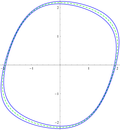
Figure 1. The transversal curves are represented in blue and the (numerical) limit cycle in dashed green, for the van der Pol system (7) with $\varepsilon=1$.

We consider the van der Pol system with $\varepsilon=1.$ The limit cycle crosses the transversal section $\Sigma$ at $x_{0}^{*}\sim 1.91928$ and it has period $T\sim 6.6632866$. We have numerically computed the limit cycle and from this approximation we have obtained the described values of $x_{0}^{*}$ and $T$.

By our method we obtain an inner transversal curve and an outer transversal curve $w_{\mbox{in}}(\theta)$ and $w_{\mbox{ex}}(\theta)$ with $\theta\in[0,2\pi]$, which provide a Poincaré–Bendixson annular region. The inner transversal curve cuts $\Sigma$ at $\sim 1.89331$ and the outer transversal curve at $\sim 1.94543$, see Figure 1.

The inner transversal curve is obtained with $\varepsilon=0.05$ and $m=12$. By the numerical computations, we obtain the following list of $n=2m+1=25$ points:

$$\begin{array}[]{l}\displaystyle\big{\{}(1.89451,0.0056435),(1.76278,-0.488101),(1.59066,-0.939363),\\ \displaystyle(1.38198,-1.33813),(1.12999,-1.67325),(0.819552,-1.92987),\\ \displaystyle(0.424859,-2.08912),(-0.093381,-2.12507),(-0.747354,-2.00013),\\ \displaystyle(-1.39679,-1.69586),(-1.80051,-1.27605),(-1.9537,-0.788939),\\ \displaystyle(-1.93903,-0.264387),(-1.83453,0.245845),(-1.68122,0.719683),\\ \displaystyle(-1.49111,1.14594),(-1.26215,1.51447),(-0.98337,1.81246),\\ \displaystyle(-0.634949,2.02302),(-0.183705,2.12466),(0.40691,2.08508),\\ \displaystyle(1.08983,1.86873),(1.63579,1.49426),(1.90318,1.04111),\\ \displaystyle(1.96187,0.527263)\big{\}}.\end{array}$$

These points are represented in Figure 2. Applying our method, we find a curve of the form (5) with $m=12,$ which passes through these points, see Figure 2.

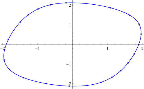
Figure 2. Points of the transversal curve to the limit cycle and the approximated transversal curve to the limit cycle of the van der Pol equation with $\varepsilon=1$, numerically computed.

For an a priori chosen precision we replace the coefficients in the above curve by rational numbers. In this particular case we obtain:

$$\displaystyle w_{1,\mbox{in}}(\theta)= \frac{1}{213892}+\frac{18566}{9395}\cos(\theta)+\frac{\cos(2\theta)}{117817}-\frac{1973}{35647}\cos(3\theta)\vspace{0.2cm}$$

$$-\frac{\cos(4\theta)}{84836}-\frac{337}{9801}\cos(5\theta)-\frac{\cos(6\theta)}{19746}+\frac{53}{5756}\cos(7\theta)\vspace{0.2cm}$$

$$-\frac{\cos(8\theta)}{420042}-\frac{\cos(9\theta)}{4738}+\frac{3\cos(10\theta)}{11954}-\frac{\cos(11\theta)}{776}+\frac{\cos(12\theta)}{5488}\vspace{0.2cm}$$

$$+\frac{1097}{13625}\sin(\theta)-\frac{\sin(2\theta)}{103485}-\frac{2003}{9487}\sin(3\theta)-\frac{\sin(4\theta)}{46332}\vspace{0.2cm}$$

$$+\frac{1317}{54185}\sin(5\theta)+\frac{\sin(6\theta)}{85313}+\frac{103}{24125}\sin(7\theta)+\frac{\sin(8\theta)}{8809}\vspace{0.2cm}$$

$$-\frac{29}{8781}\sin(9\theta)+\frac{\sin(10\theta)}{18036}+\frac{3\sin(11\theta)}{7760}-\frac{7\sin(12\theta)}{12512},$$

$$\displaystyle w_{2,\mbox{in}}(\theta)= -\frac{1}{287689}+\frac{1207\cos(\theta)}{18761}+\frac{\cos(2\theta)}{180371}-\frac{721\cos(3\theta)}{11644}\vspace{0.2cm}$$

$$+\frac{\cos(4\theta)}{46468}+\frac{116\cos(5\theta)}{18697}-\frac{\cos(6\theta)}{85239}-\frac{27\cos(7\theta)}{11035}\vspace{0.2cm}$$

$$-\frac{\cos(8\theta)}{9627}-\frac{13\cos(9\theta)}{9450}-\frac{\cos(10\theta)}{19827}+\frac{7\cos(11\theta)}{12142}\vspace{0.2cm}$$

$$+\frac{\cos(12\theta)}{2425}-\frac{22778\sin(\theta)}{10867}+\frac{\sin(2\theta)}{106711}+\frac{295\sin(3\theta)}{14827}\vspace{0.2cm}$$

$$-\frac{\sin(4\theta)}{98567}+\frac{35\sin(5\theta)}{25042}-\frac{\sin(6\theta)}{20630}-\frac{21\sin(7\theta)}{7234}+\frac{\sin(8\theta)}{3180308}\vspace{0.2cm}$$

$$+\frac{21\sin(9\theta)}{14432}+\frac{2\sin(10\theta)}{9397}+\frac{7\sin(11\theta)}{9435}+\frac{\sin(12\theta)}{5087}.$$

We know that the curve is transversal to the system if the trigonometric polynomial

$$f(\theta):=X(w_{\mbox{in}}(\theta))\cdot w_{\mbox{in}}^{\prime}(\theta)^{\perp}$$

does not change sign for all $\theta\in[0,2\pi]$. Since the polynomial $P(x,y)$ in the system is of degree $3$ and the components of $w_{\mbox{in}}(\theta)$ are of degree $12$, we have that the trigonometric polynomial $f(\theta)$ is of degree $48$. As we explained in the description of the method, we expand $f(\theta)$ in powers of $\cos\theta,\sin\theta$ and we change $\cos\theta$ by $u$ and $\sin\theta$ by $v$, in order to get a polynomial $\tilde{f}(u,v)$ which is of degree $48$. Then we take the resultant of $\tilde{f}(u,v)$ with $u^{2}+v^{2}-1$ with respect to $v$. This resultant is a polynomial in $u$ of degree $96$. Finally we prove that this polynomial has no real roots for $u\in[-1,1]$ by computing its Sturm’s sequence.

To obtain the outer transversal curve, we choose $\varepsilon=-0.05$ and $m=12$ and we repeat the process. See Figure 1 for a representation of the inner and the outer transversal curves together with the limit cycle.

4.2. Example 2: the Brusselator system

We consider the system

(8) $$\dot{x}=a-(b+1)x+x^{2}y,\quad\dot{y}=bx-x^{2}y,$$

with $a,b>0$. This system has a unique singular point at $(a,b/a)$. The semi-axis $\Sigma:=\left\{(x_{0},b/a):x_{0}>a\right\}$ is transversal to the flow. If we take $a=1$ and $b=3$, the system exhibits a hyperbolic stable limit cycle which cuts $\Sigma$ at $x_{0}^{*}\sim 2.30354344$ and has period $T\sim 7.15691986$. We have numerically computed the limit cycle and the values of $x_{0}^{*}$ and $T$ have been obtained from this approximation. By our method we obtain an inner transversal curve and an outer transversal curve, $w_{\mbox{in}}(\theta)$ and $w_{\mbox{ex}}(\theta)$ with $\theta\in[0,2\pi]$, which provide a Poincaré–Bendixson annular region. The inner transversal curve cuts $\Sigma$ at $\sim 2.2981$ and the outer transversal curve at $\sim 2.3091$, see Figure 3.

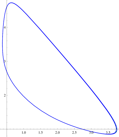
Figure 3. The transversal curves are represented in blue and the (numerical) limit cycle in dashed green for the Brusselator system with $a=1,b=3$. The three curves are almost indistinguishable.

The inner curve is obtained with $\varepsilon=0.05$ and the outer curve is obtained with $\varepsilon=-0.05$, and both of them with $m=140$. We have not been able to find a transversal curve with a lower value of $m$.

We also have considered system (8) with $a=1$ and when $b$ decreases. In this case the limit cycle shrinks until arriving to a weak focus point when $b=2$ (Hopf bifurcation). We have studied the number of points ($2m+1$) needed to construct a transversal curve with our method giving an approximation of the limit cycle with similar accuracy. When $b=2.5$ with $\varepsilon=0.02$ we need to consider $m=55$ and when $b=2.2$ with $\varepsilon=0.007$ we need $m=30$.

4.3. Comparison between the van der Pol and the Brusselator limit cycles

Recall that by using our approach we find closed transversal curves $\{w^{(m)}(\theta)\,:\,\theta\in[0,2\pi]\}$ parameterized by the angle $\theta$ given by trigonometric polynomials of degree $m$ with rational coefficients, see (5). In this section we convert these curves into $T$-periodic ones simply by considering

(9) $$W^{(m)}(t)=w^{(m)}\left(\frac{2\pi}{T}t\right).$$

As we have seen, in the van der Pol system with $\varepsilon=1$, which is

(10) $$\dot{x}=y-\left({x^{3}}/{3}-x\right),\quad\dot{y}=-x,$$

we can find a transversal curve with $\varepsilon=0.05$ and $m=12$. On the other hand, for the Brusselator system with $a=1$ and $b=3$, which is

(11) $$\dot{x}=1-4x+x^{2}y,\quad\dot{y}=3x-x^{2}y,$$

we can find a transversal curve taking $\varepsilon=0.05$ only with $m=140$ or higher. The aim of this section is to understand why the number of points to be taken, that is the value of $m$, is so different.

Before stating our main result we need to introduce some notations. If $f$ is a $T$-periodic continuous function,

$$\|f\|_{2}=\sqrt{\frac{1}{T}\int_{0}^{T}f(s)^{2}ds}\quad\mbox{and}\quad\|f\|_{\infty}=\max\{|f(s)|:s\in[0,T]\}$$

denote the $L_{2}$ and $L_{\infty}$ norms, respectively. Notice that $\|f\|_{2}\leq\|f\|_{\infty}$. When $f$ is also a class $\mathcal{C}^{1}$ function, its $\mathcal{C}^{1}$-norm is

$$||f||_{\mathcal{C}^{1}}=||f||_{\infty}+||f^{\prime}||_{\infty}.$$

Similarly, for any of the three norms, when we consider a $T$-periodic vector function $h(t)=(f(t),g(t))$, we define $||h||=||f||+||g||.$

Finally, we denote by $\mathcal{F}_{m}(f)$ the Fourier polynomial of degree $m$ associated to $f$, that is,

(12) $$\mathcal{F}_{m}(f)=\frac{a_{0}}{2}+\sum_{k=1}^{m}a_{k}\cos\left(\frac{2\pi k}{T}t\right)+b_{k}\sin\left(\frac{2\pi k}{T}t\right),$$

where the constants $a_{k},b_{k},k=0,1,2,\ldots$ are

$$a_{k}=\frac{2}{T}\int_{0}^{T}f(t)\cos\left(\frac{2\pi k}{T}t\right)\,dt,\quad b_{k}=\frac{2}{T}\int_{0}^{T}f(t)\sin\left(\frac{2\pi k}{T}t\right)\,dt.$$

Similarly $\mathcal{F}_{m}(h)=(\mathcal{F}_{m}(f),\mathcal{F}_{m}(g)).$

We collect in the next proposition some well known results of Fourier theory adapted to our interests, see for instance [9, 16]. Some of the statements hold without our strong hypotheses on $f.$

Proposition 5.

Let $f$ be a $T$-periodic $\mathcal{C}^{1}$ function. The following holds:

1. Let $p\neq\mathcal{F}_{m}(f)$ be any trigonometric polynomial of degree $m$ (that is of the form (12) with arbitrary real coefficients). Then

   $$||f-\mathcal{F}_{m}(f)||_{2}<||f-p||_{2}.$$

2. $\lim_{m\to\infty}||f-\mathcal{F}_{m}(f)||_{\mathcal{C}^{1}}=0.$

3. Plancherel’s theorem:

   $$||f||_{2}^{2}=\frac{a_{0}^{2}}{4}+\frac{1}{2}\sum_{k=1}^{\infty}\big{(}a_{k}^{2}+b_{k}^{2}\big{)}.$$

4. A consequence of Plancherel’s theorem:

   $$||f-\mathcal{F}_{m}(f)||_{2}^{2}=\frac{1}{2}\sum_{k>m}^{\infty}\big{(}a_{k}^{2}+b_{k}^{2}\big{)}\geq\frac{1}{2}\big{(}a_{m+1}^{2}+b_{m+1}^{2}\big{)}.$$

Consider the curve $\tilde{z}_{\varepsilon}(t)$ given in Theorem 2, which is strictly transversal to the flow (1). The next result shows that there always exists a trigonometric curve of the form (6) of degree $m,$ high enough, and with coefficients in $\mathbb{Q},$ which is also strictly transversal to the flow (1). Also we prove that if the Fourier series of a limit cycle $\gamma$ has a coefficient with a “high” value, then until its corresponding harmonic has been passed (that is, until we take $m$ higher than the index of this harmonic) one cannot ensure that the trigonometric curve $W^{(m)}(t)$ constructed in section 3 is near enough to the curve $\tilde{z}_{\varepsilon}(t).$ See the definition of the curve $W^{(m)}(t)$ in (9).

Theorem 6.

(i) Let $\gamma(t)=(\gamma_{1}(t),\gamma_{2}(t))$ be a $T$-periodic limit cycle of system (1). Let $|\varepsilon|>0$ be small enough, such that the $T$-periodic closed curve given in Theorem 1, $\tilde{z}_{\varepsilon}(t)$ associated to $\gamma(t)$, is strictly transversal to the flow given by (1). Then if $m=m(\varepsilon)$ is high enough, there is a $T$-periodic trigonometric curve of degree $m$ and rational coefficients which is also strictly transversal to the flow given by (1).

(ii) Taking $|\varepsilon|$ smaller, if necessary, it holds that

$$||\tilde{z}_{\varepsilon}-W^{(m)}||_{\mathcal{C}^{1}}>\frac{1}{\sqrt{2}}||\gamma_{j}-\mathcal{F}_{m}(\gamma_{j})||_{2}\geq\frac{1}{2}\sqrt{a_{m+1}^{2}+b_{m+1}^{2}},$$

where $j$ is either $1$ or $2$ and $a_{m+1}$ and $b_{m+1}$ are the coefficients of the $m+1$ harmonics of the Fourier series of $\gamma_{j}(t).$

Proof.

(i) It is clear that if $\{z(s)\,:\,s\in[0,T]\}$ and $\{\bar{z}(s)\,:\,s\in[0,T]\}\}$ are two $T$-periodic $\mathcal{C}^{1}$ closed curves, one of them is strictly transversal to the flow  (1) and $||z-\bar{z}||_{\mathcal{C}^{1}}$ is small enough, then the other curve is strictly transversal as well. By Proposition 5 (ii) it holds that for $m$ high enough there exists a $T$-periodic trigonometric polynomial curve $\tilde{W}(t)$, of degree $m$ with real coefficients and such that $||\tilde{z}_{\varepsilon}-\tilde{W}||_{\mathcal{C}^{1}}$ is as small as desired. Taking rational approximations of its coefficients with enough accuracy we get a new curve $W(t)$ that proves item (i).

(ii) Fix for instance $j=1$. We write $W^{(m)}=(W_{1}^{(m)},W_{2}^{(m)})$ where $W_{1}^{(m)}(t)=w^{(m)}_{1}\left(\frac{2\pi}{T}t\right),$ see (9). Then

$$||\tilde{z}_{\varepsilon}-W^{(m)}||_{\mathcal{C}^{1}} >||\tilde{x}_{\varepsilon}-W_{1}^{(m)}||_{\mathcal{C}^{1}}>||\tilde{x}_{\varepsilon}-W_{1}^{(m)}||_{\infty}$$

(13) $$\geq||\tilde{x}_{\varepsilon}-W_{1}^{(m)}||_{2}\geq||\tilde{x}_{\varepsilon}-\mathcal{F}_{m}(\tilde{x}_{\varepsilon})||_{2},$$

where in the last inequality we have used Proposition 5 (i), that states that the Fourier polynomial is the best approximation of a function, considering the norm $L_{2}$.

Since the curves $\tilde{z}_{\varepsilon}$ tend uniformly to $\gamma$ when $\varepsilon$ goes to zero, we have that for $|\varepsilon|$ small enough

$$||\tilde{x}_{\varepsilon}-\mathcal{F}_{m}(\tilde{x}_{\varepsilon})||_{2}>\frac{1}{\sqrt{2}}||\gamma_{1}-\mathcal{F}_{m}(\gamma_{1})||_{2}.$$

In the previous inequality we have chosen the value $1/\sqrt{2}$. We could have chosen any positive value lower than $1$. Since $x_{\varepsilon}$ tends uniformly to $\gamma_{1}$ when $\varepsilon$ goes to zero, we have that the quantity $||\tilde{x}_{\varepsilon}-\mathcal{F}_{m}(\tilde{x}_{\varepsilon})||_{2}$ is close to the quantity $||\gamma_{1}-\mathcal{F}_{m}(\gamma_{1})||_{2}$ when $\varepsilon$ tends to zero. For $|\varepsilon|$ small enough, one exceeds the other by a positive constant lower than $1$. If one takes a smaller value of $|\varepsilon|$ this constant can be reduced.

Then, from (13),

$$||\tilde{z}_{\varepsilon}-W^{(m)}||_{\mathcal{C}^{1}}>\frac{1}{\sqrt{2}}||\gamma_{1}-\mathcal{F}_{m}(\gamma_{1})||_{2}\geq\frac{1}{2}\sqrt{a_{m+1}^{2}+b_{m+1}^{2}},$$

where we have used Proposition 5 (iv). Then the theorem follows. ∎

4.4. Fourier coefficients of systems (10) and (11)

From Theorem 6 we know that for having a good enough approximation to the curve $\tilde{z}_{\varepsilon}(t)$ given in Theorem 2 by a trigonometric polynomial curve we need to consider $m$ such that the coefficients of the $m$ harmonics of the Fourier series of $\gamma(t)$ are small enough.

$m$	1	3	5-7	9	$11-13$	$15-17$	19
Coeff.	$1$	$10^{-1}$	$10^{-2}$	$10^{-3}$	$10^{-4}$	$10^{-5}$	$10^{-6}$

Table 1. Order of magnitude of the coefficients of the $m$ harmonics of the Fourier series of the first component of the limit cycle of the van der Pol system. When $m$ is even all the coefficients are zero.

$m$	$0-2$	$3-8$	$9-16$	$17-20$
Coeff.	$1$	$10^{-1}$	$10^{-2}$	$10^{-3}$

Table 2. Order of magnitude of the coefficients of the $m$ harmonics of the Fourier series of the first component of the limit cycle of the Brusselator system.

Therefore the number of points $n=2m+1$ used to construct our curve $W^{(m)}(t)$ is strongly related with the size of the Fourier coefficients of $\gamma(t)$. These coefficients can be numerically obtained before starting our process for obtaining a Poincaré annular region for proving the existence of a periodic orbit. In Tables 1 and 2 we show the order of magnitude of them for the first component $\gamma_{1}(t)$ of the limit cycles $\gamma(t)$ of the van der Pol (10) and the Brusselator (11) systems. The results for the second component are essentially the same. Notice that the modulus of the coefficients of the harmonics in the Brusselator system descend much more slowly than in the van der Pol system, giving a clear explanation of the harder difficulty for finding trigonometric curves without contact for the Brusselator system.

5. The Rychkov system

The aim of this section is to prove Theorem 3. As we have already said in the introduction we consider the system studied by Rychkov in 1975, see [13],

(14) $$\dot{x}=y-\left(x^{5}-\mu x^{3}+\delta x\right),\quad\dot{y}=-x,$$

with $\delta,\mu\in\mathbb{R}$. The semi-axis $\Sigma:=\left\{(x_{0},0)\in\mathbb{R}^{2}:x_{0}>0\right\}$ is a transversal section. This system is also studied in [1, 8, 10]. The following features of system (14) can be found in the aforementioned references. The origin is the only finite singular point and it is a focus. Rychkov [13] proved that it has at most two limit cycles and that for $\delta<0$ there exists a unique limit cycle, which is stable. The line $\delta=0$ is a curve of occurrence of Hopf bifurcations. When $\mu>0$ there is a curve of bifurcation values $\delta=\Delta(\mu)$ of a saddle-node bifurcation of limit cycles. Odani [10] proved that if $\delta>0$ and $0<\delta<\mu^{2}/5$, then the system has two limit cycles. Figure 4 represents the bifurcation diagram of the Rychkov system (14) in the $(\delta,\mu)$-plane.

Figure 4. Bifurcation diagram of the Rychkov system (14). The curve of the saddle-node bifurcation is qualitative.

Here we fix $\mu=1$ and we are interested in finding sharp bounds for $\delta^{*}=\Delta(1)$. Since the Rychkov system is a semi-complete family of rotated vector fields with respect to $\delta$, see [3, 11, 12] it holds that:

• It for $\delta=\bar{\delta}$ the system has two limit cycles then $\bar{\delta}<\delta^{*}.$ Therefore, to prove the inequality $0.224\,{<}\,\delta^{*}$, it suffices to prove that the Rychkov system has two limit cycles for $\delta=0.224.$

• Similarly, if for $\delta=\hat{\delta}$ the system has no limit cycle then $\delta^{*}<\hat{\delta}.$ Then, to prove the inequality $\delta^{*}<\,\,0.2249654$, it suffices to prove that the Rychkov system has no limit cycle for $\delta=\,0.2249654.$

Therefore, the proof of Theorem 3 can be reduced to the study of the above two given values of $\delta$. We study each case in a different subsection.

5.1. The proof that system (3) has two limit cycles for $\delta=0.224$

Although it suffices to study the case $\delta=0.224$, we prefer to study also the smaller values of $\delta,$ $0.2$ and $0.22$ to see how the two limit cycles evolve with the parameter. In the three cases, the origin is a strong stable focus, the smaller limit cycle is hyperbolic and unstable and the bigger limit cycle is hyperbolic and stable.

5.1.1. The case $\delta=0.2$

The limit cycles cut $\Sigma$ at $x_{0}\sim 0.632018$ and $x_{0}\sim 0.893787$. By our method we have been able to construct three transversal curves which provide two Poincaré–Bendixson regions. These regions allow to locate each one of the limit cycles. The interior transversal curve cuts $\Sigma$ at $x_{0}=0.474059$, it has been obtained from the unstable limit cycle taking $\varepsilon=0.1$ and $m=5$. The transversal curve in the middle cuts $\Sigma$ at $x_{0}=0.711158$, it has been obtained from the unstable limit cycle taking $\varepsilon=-0.05$ and $m=7$. The exterior transversal curve cuts $\Sigma$ at $x_{0}=1.00597$, it has been obtained from the stable limit cycle taking $\varepsilon=-0.1$ and $m=5$. These curves, together with the limit cycles are represented in Figure 5.

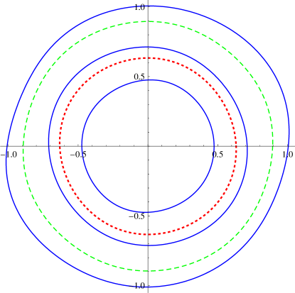
Figure 5. Transversal curves are represented in blue and the limit cycles in dotted red (unstable) and dashed green (stable) for the Rychkov system with $\mu=1$ and $\delta=0.2$.

5.1.2. The case $\delta=0.22$

In this case the limit cycles cut $\Sigma$ at $x_{0}\sim 0.714276$ and $x_{0}\sim 0.830266$. The interior transversal curve cuts $\Sigma$ at $x_{0}=0.57421$, it has been obtained from the unstable limit cycle taking $\varepsilon=0.1$ and $m=7$. The transversal curve in the middle cuts $\Sigma$ at $x_{0}=0.74227$, it has been obtained from the unstable limit cycle taking $\varepsilon=-0.02$ and $m=7$. The exterior transversal curve cuts $\Sigma$ at $x_{0}=0.8905$, it has been obtained from the stable limit cycle taking $\varepsilon=-0.05$ and $m=7$.

5.1.3. The case $\delta=0.224$

For this value of $\delta$ the limit cycles cut $\Sigma$ at $x_{0}\sim 0.748705$ and $x_{0}\sim 0.799588$. As in the previous case, we have been able to find three transversal curves which analytically prove the existence of the two limit cycles. The interior transversal curve cuts $\Sigma$ at $x_{0}=0.615043$, it has been obtained from the unstable limit cycle taking $\varepsilon=0.1$ and $m=7$. The transversal curve in the middle cuts $\Sigma$ at $x_{0}=0.75939$, it has been obtained from the unstable limit cycle taking $\varepsilon=-0.008$ and $m=10$. The exterior transversal curve cuts $\Sigma$ at $x_{0}=0.862111$, it has been obtained from the stable limit cycle taking $\varepsilon=-0.05$ and $m=7$. See Figure 6.

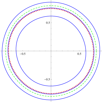
Figure 6. Transversal curves are represented in blue and the limit cycles in dotted red (unstable) and dashed green (stable) for the Rychkov system with $\mu=1$ and $\delta=0.224$.

5.2. The proof that system (3) has no limit cycle for $\delta=0.2249654$

Before proving the second part of the theorem we need some preliminary results.

The first lemma recalls a classical method for proving non-existence of periodic orbits. We state and prove it on the plane, but notice that it works in any dimension.

Lemma 7.

Let $\mathcal{U}$ be an open subset of $\mathbb{R}^{2}$ and let $B:\mathcal{U}\to\mathbb{R}$ be a class $\mathcal{C}^{1}$ function such that its total derivative with respect to the flow (1),

$$\dot{B}(x,y)=\nabla B(x,y)\cdot X(x,y)=\frac{\partial B(x,y)}{\partial x}P(x,y)+\frac{\partial B(x,y)}{\partial y}Q(x,y)$$

does not change sign on $\mathcal{U}$ and vanishes on a set of zero Lebesgue measure which is not invariant by the flow of (1). Then the system (1) has not periodic orbits totally contained in $\mathcal{U}.$

Proof.

Let $z(t)=(x(t),y(t))$ be any solution of (1), contained in $\mathcal{U}$ for $t\in[t_{1},t_{2}],$ $t_{1}<t_{2}.$ Then,

$$0\neq\int_{t_{1}}^{t_{2}}\dot{B}(z(t))\,dt=B(z(t_{2}))-B(z(t_{1}).$$

Hence the orbit cannot be periodic, as we wanted to prove. ∎

The next result is an adaptation of [2, Thm. 3] to our interests. We sketch its proof.

Proposition 8.

([2]) Given a classical polynomial Liénard system

(15) $$\dot{x}=y-F(x),\quad\dot{y}=-x$$

and $n\in\mathbb{N}$, there exists a unique polynomial $B_{n}(x,y)=\sum_{i=0}^{n}B_{i}(x)y^{i}$ such that $B_{n}(0,y)=y^{n}$ and its total derivative with respect to (15) is a polynomial that does not depend on $y.$

Proof.

We have that

$$\dot{B}_{n}(x,y)= \frac{\partial B_{n}(x,y)}{\partial x}\big{(}y-F(x)\big{)}-x\,\frac{\partial B_{n}(x,y)}{\partial y}$$

$$= \,\,\Big{(}\sum_{i=0}^{n}B_{i}^{\prime}(x)y^{i}\Big{)}\big{(}y-F(x)\big{)}-x\,\sum_{i=1}^{n}i\,B_{i}(x)y^{i-1}$$

$$= \,\,B_{n}^{\prime}(x)y^{n+1}+\big{(}B_{n-1}^{\prime}(x)-F(x)B^{\prime}_{n}(x)\big{)}y^{n}$$

$$+\sum_{k=1}^{n-1}\Big{(}B_{k-1}^{\prime}(x)-F(x)B_{k}^{\prime}(x)-(k+1)xB_{k+1}(x)\Big{)}y^{k}$$

$$-F(x)B_{0}^{\prime}(x)-xB_{1}(x).$$

We impose the conditions $B_{n}(0)=1,B_{k}(0)=0$ for $k=0,1,\ldots,n-1.$ Then we can solve step by step the trivial linear differential equations given by the vanishing of the coefficients of $y^{n+1},y^{n},\ldots$ until $y$. We obtain that $B_{n}(x)\equiv 1,$ $B_{n-1}(x)\equiv 0,$ $B_{n-2}(x)=nx^{2}/2$,

$$B_{n-3}(x)=n\int_{0}^{x}sF(s)\,ds,\quad B_{n-4}(x)=n\int_{0}^{x}sF^{2}(s)\,ds+\frac{n(n-2)}{8}x^{4}$$

and so on. Finally $\dot{B}(x,y)=-F(x)B_{0}^{\prime}(x)-xB_{1}(x),$ as we wanted to prove. ∎

The proof that the Rychkov system with $\mu=1$ and $\delta=0.2249654$ has no limit cycle. Applying Proposition 8 to system (3),

$$\dot{x}\,=\,y-\left(x^{5}-x^{3}+\delta x\right),\quad\dot{y}\,=\,-x,$$

we get that

$$\dot{B}_{n}(x,y)=x^{n}R_{4(n-1)}(x,\delta),$$

where $R_{4(n-1)}$ is an even polynomial in $x$ of degree $4(n-1).$ For instance, taking $n=4$ we get that

$$B_{4}(x,y)= y^{4}+2x^{2}y^{2}+\frac{4}{105}x^{3}\left(15x^{4}-21x^{2}+35\delta\right)y$$

$$+\frac{1}{30}x^{4}\left(10x^{8}-24x^{6}+30\delta x^{4}+15x^{4}-40\delta x^{2}+30\delta^{2}+30\right)$$

and

$$R_{12}(x,\delta)=-\frac{4}{105}\Big{(} 105{x}^{12}-315{x}^{10}+\left(315\delta+315\right){x}^{8}$$

$$-\left(630\delta+105\right){x}^{6}+\left(315{\delta}^{2}+315\delta+120\right){x}^{4}$$

$$-\left(315{\delta}^{2}+126\right){x}^{2}+35\delta\left(3{\delta}^{2}+4\right)\Big{)}.$$

The discriminant of the above polynomial with respect to $x$, except for some non-zero rational constant factor, is

$$\delta\big{(}3{\delta}^{2}+4\big{)}\Big{(} 4233600000{\delta}^{7}-4953312000{\delta}^{6}+59568485760{\delta}^{5}$$

$$-65416468320{\delta}^{4}+256186378380{\delta}^{3}-171344748015{\delta}^{2}$$

$$+250762344740\delta-52896972996\Big{)}^{2}.$$

By using once more the Sturm’s approach we can prove that it only has one positive zero at $\delta=\delta_{4}\approx 0.2362516\ldots.$ Therefore, it is not difficult to prove that if $\delta\geq 0.236252$ then $R_{12}(x,\delta)<0.$ In fact, for our interests it suffices to prove that $R_{12}(x,0.236252)<0$ for all $x\in\mathbb{R}.$ From this fact, for $\delta=0.236252$, we have $\dot{B}_{4}(x,y)\leq 0,$ and it vanishes only at $x=0$. Then, by Lemma 7 we know that for this value of $\delta$ the system (3) has no limit cycle. As a consequence we have that $\delta^{*}<0.236252.$

Repeating the above procedure for different values of $n$ (even) we improve the upper bound for $\delta^{*}$. Our results are presented in Table 3.

$n$	$50$	$100$	$150$	$200$	$250$	$300$
Bound	$0.2252$	$0.2251$	$0.2250$	$0.2249715$	$0.2249676$	$0.2249654$

Table 3. Upper bounds for $\delta^{*}$ for the Rychkov system (3) with $\mu\,=\,1$.

It is remarkable that increasing $n\leq 300$ we have found that there exist values $\delta_{n}$ such that for $\delta>\delta_{n}$ it holds that $R_{4(n-1)}(x,\delta)<0$ and moreover that these values seem to decrease monotonically towards $\delta^{*}.$ Observe also that for the case $n=300$ we must prove that the even polynomial of degree 1196, $R_{1196}(x,0.2249654),$ which has rational coefficients, has no real roots. ∎

References

- [1] P. Alsholm, Existence of limit cycles for generalized Liénard equations. J. Math. Anal. Appl. 171 (1992), 242–255.
- [2] L.A. Cherkas, Estimation of the number of limit cycles of autonomous systems. Differ. Uravn. 13 (1977) 779–802; translation in Differ. Equ. 13 (1977) 529–547.
- [3] G.F.D. Duff, Limit-cycles and rotated vector fields. Ann. of Math. 57 (1953) 15–31.
- [4] M.P. do Carmo, Differential geometry of curves and surfaces. Translated from the Portuguese. Prentice-Hall, Inc., Englewood Cliffs, N.J., 1976.
- [5] F. Dumortier, J. Llibre and J.C. Artés, Qualitative theory of planar differential systems. Universitext. Springer Verlag, Berlin, 2006.
- [6] H. Giacomini and M. Grau, Transversal conics and the existence of limit cycles, J. Math. Anal. Appl. 428 (2015), 563–586.
- [7] H. Giacomini and S. Neukirch, Number of limit cycles of the Liénard equation, Phys. Rev. E 56 (1997) 3809–3813.
- [8] H. Giacomini and S. Neukirch, Algebraic approximations to bifurcation curves of limit cycles for the Liénard equation. Phys. Lett. A 244 (1998), 53–58.
- [9] T.W. Körner, Fourier analysis. Second edition. Cambridge University Press, Cambridge, 1989.
- [10] K. Odani, Existence of exactly periodic solutions for Liénard systems. Funkcial. Ekvac. 39 (1996), 217–234.
- [11] L.M. Perko, Rotated vector fields. J. Differential Equations 103 (1993), 127–145.
- [12] L.M. Perko, Differential equations and dynamical systems. Third edition. Texts in Applied Mathematics, 7. Springer-Verlag, New York, 2001.
- [13] G.S. Rychkov, The maximum number of limit cycles of polynomial Liénard systems of degree five is equal to two. Differential Equations, 11 (1975), 301–302.
- [14] J. Stoer and R. Bulirsch, Introduction to numerical analysis. Translated from the German by R. Bartels, W. Gautschi and C. Witzgall. Springer-Verlag, New York-Heidelberg, 1980.
- [15] B. Sturmfels, Solving Systems of Polynomial Equations, CBMS Reg. Conf. Ser. Math., vol.97, American Mathematical Society, Providence, RI, 2002, Published for the Conference Board of the Mathematical Sciences, Washington, DC.
- [16] G.P. Tolstov, Fourier series. Second English translation. Translated from the Russian and with a preface by Richard A. Silverman. Dover Publications, Inc., New York, 1976.
- [17] Ye Yan Qian and others, Theory of limit cycles. Translations of Mathematical Monographs, 66. American Mathematical Society, Providence, RI, 1986.
- [18] Zhi Fen Zhang and others Qualitative theory of differential equations. Translations of Mathematical Monographs, 101. American Mathematical Society, Providence, RI, 1992.