On the Chiral imbalance and Weibel Instabilities

Abstract

We study the chiral-imbalance and the Weibel instabilities in presence of the quantum anomaly using the Berry-curvature modified kinetic equation. We argue that in many realistic situations, e.g. relativistic heavy-ion collisions, both the instabilities can occur simultaneously. The Weibel instability depends on the momentum anisotropy parameter $\xi$ and the angle ($\theta_{n}$) between the propagation vector and the anisotropy direction. It has maximum growth rate at $\theta_{n}=0$ while $\theta_{n}=\pi/2$ corresponds to a damping. On the other hand the pure chiral-imbalance instability occurs in an isotropic plasma and depends on difference between the chiral chemical potentials of right and left-handed particles. It is shown that when $\theta_{n}=0$, only for a very small values of the anisotropic parameter $\xi\sim\xi_{c}$, growth rates of the both instabilities are comparable. For the cases $\xi_{c}<\xi\ll 1$, $\xi\approx 1$ or $\xi\geq 1$ at $\theta_{n}=0$, the Weibel modes dominate over the chiral-imbalance instability if $\mu_{5}/T\leq 1$. However, when $\mu_{5}/T\geq 1$, it is possible to have dominance of the chiral-imbalance modes at certain values of $\theta_{n}$ for an arbitrary $\xi$.

The scope of applying kinetic theory to understand variety of many-body problems arising in various branches of physics is truly enormous [1]. The conventional Boltzmann or Vlasov equations imply that the vector current associated with the gauge charges is conserved. But till recently a very important class of physical phenomena associated with the CP-violation or the triangle-anomaly were left out of the purview of a kinetic theory. In such a phenomenon the axial current is not conserved. It should be noted here that there exists a several models of hydrodynamics which incorporates the effect of CP-violation [2, 3, 4, 5]. But a hydrodynamical approach requires that the system under consideration remains in a thermal and chemical equilibrium. However, many applications of the chiral (CP-violating) physics may involve a non-equilibrium situation e.g. during the early stages of relativistic heavy-ion collisions. Therefore it is highly desirable to have a proper kinetic theory framework to tackle the CP-violating effect. Recently there has been a lot of progress in developing such a kinetic theory. In Ref. [6, 7, 8, 9, 10, 11] it was shown that if the Berry curvature[12] has nonzero flux across the Fermi-surface then the particles on the surface can exhibit a chiral anomaly in presence of an external electromagnetic field. In this formalism chiral-current $j^{\mu}$ is not conserved and it can be attributed to Adler-Bell-Jackiw anomaly [13, 14, 15]. It can be shown that if a system of charged fermions does not conserve parity, it can develop an equilibrium electric current along an applied external magnetic field [16]. This is so called chiral-magnetic effect (CME). It has been suggested that a strong magnetic field created in relativistic-heavy-ion experiments can lead to CME in the quark-gluon plasma [17, 18, 19]. Indeed the recent experiments with STAR detector at Relativistic Heavy Ion Collider (RHIC) qualitatively agree with a local parity violation. However, more investigations are required to attribute this charge asymmetry with the CME [20, 21]. The idea that a Berry-phase can influence the electronic properties [e.g. [22] and references cited therein] is well-known in condensed matter literature and it can have applications in Weyl semimetal [23], graphene [24] etc. There exists a deep connection between a CP-violating quantum field theory and the kinetic theory with the Berry curvature corrections. In Ref. [25] it was shown that the parity-odd and parity-even correlations calculated using the modified kinetic theory are identical with the perturbative results obtained in next-to-leading order hard dense loop approximation.

In this work we aim to apply the kinetic theory with the Berry curvature corrections to some non-equilibrium situations. We first note that the results obtained in Refs. [6, 25] are limited to low temperature regime $T\ll\mu_{5}$, where $\mu_{5}$ is chiral chemical potential, when the Fermi surface is well-defined. Recently Ref.[26] argues that the domain of validity of the modified kinetic theory can be extended beyond the Fermi surface to include the effect of finite temperature. As expected from the considerations of quantum-field theoretic approach [27, 28, 29] the parity-odd contribution remains temperature independent. Recently using the modified-kinetic theory [25] in presence of the chiral imbalance the collective modes in electromagnetic or quark-gluon plasmas were analyzed [30]. In such a system CP-violating effect can split transverse waves into two branches [31]. It was found in Ref. [30] that in the quasi-static limit i.e. for $\omega\ll k$, where $\omega$ and $k$ respectively denote frequency and wave-number of the transverse wave, there exists an unstable mode. The instability can lead to the growth of Chern-Simons number (or magnetic-helicity in plasma physics parlance) at expense of the chiral imbalance. Similar kind of instabilities were found in Refs. [32, 33, 34, 35, 36] in different context.

It may be possible to observe the instability reported in Ref. [30] in the relativistic heavy-ion collisions. But in a realistic scenario the initial distribution function $n^{0}_{\bf p}$ for the strongly interacting matter formed during the collision can be anisotropic in the momentum space. This kind of initial distribution known to lead to the Weibel instability of the transverse modes. In the context of relativistic heavy-ion collision experiments Weibel instability has been extensively studied [37, 38, 39, 40, 41]. The Weibel instability is also well-known in the condensed matter [42, 43] and plasma physics literatures [44, 45, 46] and it can generate magnetic fields in the plasma. Further it should be emphasized that both the chiral-imbalance and the Weibel instability can operate in the quasi-static regime. Therefore in the present work we aim to analyze the collective modes in an anisotropic chiral plasma and study how the chiral-imbalance and Weibel instabilities can influence each other. We believe that the results presented here will be useful in studying Weyl metals and the quark-gluon plasma created in relativistic heavy-ion collisions. We consider weak gauge Field limit and assume the following power counting scheme: $\partial_{x}=O(\delta)$ and $A^{\mu}=O(\epsilon)$. Here, $\epsilon$ and $\delta$ are small independent parameters. In this senario we use modified collisonless kinetic (Vlasov) equation at the leading order in $A^{\mu}$ as given in Ref. [25]:

$$(\partial_{t}+{\mathbf{v}}\cdot{\mathbf{\partial_{x}}})n_{\mathbf{p}}+(e{\mathbf{E}}+e{\mathbf{v}}\times{\mathbf{B}}-{{\mathbf{\partial}}_{\mathbf{x}}}\mathbf{\epsilon_{p}})\cdot{\mathbf{\partial}}_{\mathbf{p}}n_{\mathbf{p}}=0$$ (1)

where $\mathbf{v}=\frac{\bf{p}}{p}$, $\mathbf{\epsilon_{p}}=p(1-e{\mathbf{B\cdot\Omega_{p}}})$ and ${\mathbf{\Omega_{p}}}=\pm{\mathbf{p}}/{2p^{3}}$. Here $\pm$ sign corresponds to right and lefted handed fermions respectively. In absence of the Berry curvature term (i.e. $\Omega_{\bf p}$=0) $\epsilon_{\bf{p}}$ is independent of x, Eq.(1) reduces to the standard Vlasov equation.

In this case current density $\bf j$ is defined as:

$${\bf j}=-e\int\frac{d^{3}p}{(2\pi)^{3}}\Big{[}\epsilon_{\bf p}{\mathbf{\partial}}_{\mathbf{p}}n_{\mathbf{p}}+e\left({\bf\Omega}_{\bf p}\cdot{\mathbf{\partial}}_{\mathbf{p}}n_{\mathbf{p}}\right)\epsilon_{\bf p}{\bf B}$$ (2)

$$+\epsilon_{\bf p}{\bf\Omega}_{\bf p}\times{\mathbf{\partial}}_{\mathbf{x}}n_{\mathbf{p}}\Big{]}+e{\bf E}\times{\bf\sigma},$$

where ${\mathbf{\partial}}_{\mathbf{P}}=\frac{\partial}{\partial{\bf p}}$ and ${\mathbf{\partial}}_{\mathbf{x}}=\frac{\partial}{\partial{\bf x}}$. The last term on the right hand side of the above equation represents the anomalous Hall current with $\sigma$ given as follows:

$${\bf\sigma}=e\int\frac{d^{3}p}{(2\pi)^{3}}{\bf\Omega}_{\bf p}n_{\bf p}.$$ (3)

Using Maxwell’s equations and linear response theory it is easy to write down the expression for the inverse of the propagator in temporal gauge $A_{0}=0$ as follows,

$$[({k^{2}}-{\omega}^{2})\delta^{ij}-k^{i}k^{j}+\Pi^{ij}(K)]E^{j}=[\Delta^{-1}(K)]^{ij}E^{j}=i\omega{j^{i}_{ext}}(k).$$ (4)

Here, $\Pi^{ij}(K)$ is the retarded self energy which follows from expression of the induced current $j^{\mu}_{ind}=\Pi^{\mu\nu}(K)A_{\nu}(K)$ and $[\Delta^{-1}(K)]^{ij}$ is the inverse of the propagator. Dispersion relation can be obtained by finding the poles of the propagator $[\Delta(K)]^{ij}$.

Let us first concentrate on right handed fermions with chemical potential $\mu_{R}$. We consider the background distribution of the form $n^{0}_{\mathbf{p}}=1/[e^{(\mathbf{\epsilon_{p}}-\mu_{R})/T}+1]$. In a linear response theory we are interested in the induced current by a linear-order deviation in the gauge field. We follow the power counting scheme for gauge field $A_{\mu}$ and derivatives $\partial_{x}$ as discussed earlier, and consider deviations in the current and the distribution function up to $O(\epsilon\delta)$. In this case we can write the distribution in Eq.(1) as follows,

$$n_{\mathbf{p}}=n^{0}_{\mathbf{p}}+e(n^{(\epsilon)}_{\mathbf{p}}+n^{(\epsilon\delta)}_{\mathbf{p}})$$ (5)

where, $n^{0}_{\mathbf{p}}$ is the background distribution function in presence of Berry curvature while $n^{(\epsilon)}_{\mathbf{p}}$ and $n^{(\epsilon\delta)}_{\mathbf{p}}$ are the pertubations of order $O(\epsilon)$ and $O(\epsilon\delta)$ around $n^{0}_{\mathbf{p}}$. Since $n^{0}_{\mathbf{p}}$ contains the Berry curvature contribution (Due to $\epsilon_{\mathbf{p}}$) therefore, can also be splitted into order $O(0)$ and $O(\epsilon\delta)$ i.e., $n^{0}_{\mathbf{p}}=n^{0(0)}_{\mathbf{p}}+en^{0(\epsilon\delta)}_{\mathbf{p}}$, where $n^{0(0)}_{\mathbf{p}}=\frac{1}{[e^{(p-\mu_{R})/T}+1]}$ is the part of background distribution function without Berry curvature correction while $n^{0(\epsilon\delta)}_{\mathbf{p}}=\left(\frac{{\mathbf{B}\cdot\mathbf{v}}}{2pT}\right)\frac{e^{(p-\mu_{R})/T}}{[e^{(p-\mu_{R})/T}+1]^{2}}$ is the part of background distribution with Berry curvature correction. In order to bring in effect of anisotropy we follow the arguments of Ref. [41]. It is assumed that the anisotropic equilibrium distribution function can be obtained from a spherically symmetric distribution function by rescaling of one direction in the momentum space. We consider that there is a momentum anisotropy in direction of a unit vector ${\mathbf{\hat{n}}}$. Noting that $p=|{\mathbf{p}}|$, we replace $p\rightarrow\sqrt{{\mathbf{p}}^{2}+\xi({\mathbf{p}}\cdot{\mathbf{\hat{n}}})^{2}}$ in the expression of $n^{0}_{\mathbf{p}}$ to get anisotropic distribution function. Here $\xi$ is an adjustable anisotropy parameter satisfying a condition $\xi>-1$. It is convenient to define a new variable $\tilde{p}$ such that $\tilde{p}=p\sqrt{1+\xi({\mathbf{v}}\cdot{\mathbf{\hat{n}}})^{2}}$. Using this new variable one can write $n^{0(0)}_{\mathbf{p}}=\frac{1}{[e^{(\tilde{p}-\mu_{R})/T}+1]}$ and $n^{0(\epsilon\delta)}_{\mathbf{p}}=\left(\frac{{\mathbf{B}\cdot\mathbf{v}}}{2\tilde{p}T}\right)\frac{e^{(\tilde{p}-\mu_{R})/T}}{[e^{(\tilde{p}-\mu_{R})/T}+1]^{2}}$.

The anomalous Hall current term in Eq.(2) can vanish if the distribution function is spherically symmetric in the momentum space. However, for an anisotropic distribution function this may not be true in general. Since the Hall-current term depends on electric field, it can be of order $O(\epsilon\delta)$ or higher. As we are interested in finding deviations in current and distribution function up to order $O(\epsilon\delta)$, only $n^{0(0)}_{\mathbf{p}}$ would contribute to the Hall current term. Next, we consider ${\bf\sigma}$ from Eq.(3) which can be written as

$${\bf\sigma}=\frac{e}{2}\int d\Omega d\tilde{p}\frac{\mathbf{v}}{[1+\xi(\mathbf{v}\cdot\mathbf{\hat{n}})]^{1/2}}\frac{1}{(1+e^{(\tilde{p}-\mu_{R})/T})}.$$ (6)

Since $\mathbf{v}$ is a unit vector one can express $\mathbf{v}=(sin\theta cos\phi,sin\theta sin\phi,cos\theta)$ in spherical coordinates. By choosing $\mathbf{\hat{n}}$ in $z-$direction, without any loss of generality, one can have $\mathbf{v}\cdot\mathbf{\hat{n}}=cos\theta$. Thus the angular integral in the above equation becomes $\int d(cos\theta)d\phi\frac{\mathbf{v}}{(1+\xi cos^{2}\theta)^{1/2}}$. Therefore $\sigma_{x}$ and $\sigma_{y}$ components of Eq.(6) will vanish as $\int^{2\pi}_{0}sin\phi d\phi=0$ and $\int^{2\pi}_{0}cos\phi d\phi=0$. While $\sigma_{z}$ will vanish because integration with respect to $\cos\theta$ variable will yield it ($\sigma_{z}$) to be zero. Thus the anomalous Hall current term will not contribute for the problem at the hand.

Now the kinetic equation (1) can be split into two equations valid at $O(\epsilon)$ and $O(\epsilon\delta)$ scales of distribution function as written below,

$$(\partial_{t}+{\mathbf{v}}\cdot{\mathbf{\partial_{x}}})n^{(\epsilon)}_{\mathbf{p}}=-({\mathbf{E}}+{\mathbf{v}}\times{\mathbf{B}})\cdot{\mathbf{\partial}}_{\mathbf{p}}n^{0(0)}_{\mathbf{p}}$$ (7)

$$(\partial_{t}+{\mathbf{v}}\cdot{\mathbf{\partial_{x}}})(n^{0(\epsilon\delta)}_{\mathbf{p}}+n^{(\epsilon\delta)}_{\mathbf{p}})=-\frac{1}{e}{{{\mathbf{\partial}}_{\mathbf{x}}}\mathbf{\epsilon_{p}}}\cdot{\mathbf{\partial}}_{\mathbf{p}}{n^{0(0)}_{\mathbf{p}}}$$ (8)

Equation for the current defined in Eq.(2) can also split into $O(\epsilon)$ and $O(\epsilon\delta)$ scales as given below,

$$\mathbf{j^{\mu(\epsilon)}}=e^{2}\int\frac{d^{3}p}{(2\pi)^{3}}v^{\mu}n^{(\epsilon)}_{\mathbf{p}}$$ (9)

$$\mathbf{j^{i(\epsilon\delta)}}=e^{2}\int\frac{d^{3}p}{(2\pi)^{3}}\left[v^{i}n^{(\epsilon\delta)}_{\mathbf{p}}-\left(\frac{{v^{j}}}{2p}\frac{\partial{n^{0(0)}_{\mathbf{p}}}}{\partial{p^{j}}}\right){{B^{i}}}-\epsilon^{ijk}\frac{v^{j}}{2p}\frac{\partial{n^{(\epsilon)}_{\mathbf{p}}}}{\partial{x^{k}}}\right]$$ (10)

After adding the contribution from all type of species i.e. right/left fermions with charge $e$ and chemical potential $\mu_{R}/\mu_{L}$ as well as right/left handed antifermions with charge $-e$ and chemical potential $-\mu_{R}/\mu_{L}$, using the expression $j^{\mu}_{ind}=\Pi^{\mu\nu}(K)A_{\nu}(K)$ and Eqs. (7, 8, 9, 10) one can obtain the expression for self energy, $\Pi^{ij}=\Pi^{ij}_{+}+\Pi^{ij}_{-}$. The expressions for $\Pi^{ij}_{+}$ (parity even part of polarization tensor) and $\Pi^{ij}_{-}$ (parity-odd part) can be written as,

$${\Pi^{ij}_{+}(K)}=m^{2}_{D}\int\frac{d\Omega}{4\pi}\frac{{v^{i}}({v^{l}}+\xi(\mathbf{v\cdot{\hat{n}}})\hat{n}^{l})}{(1+\xi(\mathbf{v\cdot{\hat{n}}})^{2})^{2}}\left(\delta^{jl}+\frac{v^{j}k^{l}}{{\bf{v\cdot k}}+i\epsilon}\right),$$ (11)

$${\Pi^{im}_{-}(K)}=C_{E}\int\frac{d\Omega}{4\pi}\Bigg{[}\frac{i{\epsilon}^{jlm}k^{l}v^{j}v^{i}(\omega+\xi(\bf{v\cdot\hat{n}})(\bf{k\cdot\hat{n}}))}{({\bf{v\cdot k}}+i{\epsilon})(1+\xi(\mathbf{v\cdot{\hat{n}}})^{2})^{3/2}}+$$

$$\left(\frac{{v^{j}}+\xi(\mathbf{v\cdot{\hat{n}}})\hat{n}^{j}}{(1+\xi(\mathbf{v\cdot{\hat{n}}})^{2})^{3/2}}\right){i{\epsilon}^{iml}k^{l}v^{j}}$$

$$-{i{\epsilon}^{ijl}k^{l}v^{j}}\left(\delta^{mn}+\frac{v^{m}k^{n}}{{\bf{v\cdot k}}+i\epsilon}\right)\left(\frac{{v^{n}}+\xi(\mathbf{v\cdot{\hat{n}}})\hat{n}^{n}}{(1+\xi(\mathbf{v\cdot{\hat{n}}})^{2})^{3/2}}\right)\Bigg{]}$$ (12)

where,

$$m^{2}_{D}=-\frac{e^{2}}{2\pi^{2}}\int_{0}^{\infty}d\tilde{p}{\tilde{p}}^{2}\Bigg{[}\frac{\partial{n^{0(0)}_{\mathbf{\tilde{p}}}}(\tilde{p}-\mu_{R})}{\partial{\tilde{p}}}+\frac{\partial{n^{0(0)}_{\mathbf{\tilde{p}}}}(\tilde{p}+\mu_{R})}{\partial{\tilde{p}}}$$

$$+\frac{\partial{n^{0(0)}_{\mathbf{\tilde{p}}}}(\tilde{p}-\mu_{L})}{\partial{\tilde{p}}}+\frac{\partial{n^{0(0)}_{\mathbf{\tilde{p}}}}(\tilde{p}-\mu_{L})}{\partial{\tilde{p}}}\Bigg{]}$$

$$C_{E}=-\frac{e^{2}}{4\pi^{2}}\int_{0}^{\infty}d\tilde{p}{\tilde{p}}\Bigg{[}\frac{\partial{n^{0(0)}_{\mathbf{\tilde{p}}}}(\tilde{p}-\mu_{R})}{\partial{\tilde{p}}}-\frac{\partial{n^{0(0)}_{\mathbf{\tilde{p}}}}(\tilde{p}+\mu_{R})}{\partial{\tilde{p}}}$$

$$-\frac{\partial{n^{0(0)}_{\mathbf{\tilde{p}}}}(\tilde{p}-\mu_{L})}{\partial{\tilde{p}}}+\frac{\partial{n^{0(0)}_{\mathbf{\tilde{p}}}}(\tilde{p}-\mu_{L})}{\partial{\tilde{p}}}\Bigg{]}.$$ (13)

We would like to mention that the total induced current is, $\bf{j}=\bf{j}^{\epsilon}+\bf{j}^{\epsilon\delta}$ where, $\bf{j}^{\epsilon}$ gives contribution of the order of the square of plasma frequency or $m^{2}_{D}$. The plasma frequency contains additive contribution from the densities of all species i.e. right-handed particle/antiparticles and left-handed particles/antiparticles. The current $\bf{j}^{\epsilon\delta}$ arises due to chiral imbalance its contribution from each plasma specie, depends upon $e\vec{\Omega_{p}}$. Since $e\vec{\Omega_{p}}$ can change sign depending on the plasma specie therefore definition of $C_{E}$ contains both positive and negative signs. Consequently a relative signs of fermion and anti-fermion are different in $m^{2}_{D}$ and $C_{E}$. After performing above integrations one can get $m^{2}_{D}=e^{2}\left(\frac{\mu_{R}^{2}+\mu_{L}^{2}}{2\pi^{2}}+\frac{T^{2}}{3}\right)$ and $C_{E}=\frac{e^{2}\mu_{5}}{4\pi^{2}}$, where $\mu_{5}=\mu_{R}-\mu_{L}$. It should be emphasized here that $C_{E}=0$ when there is no chiral imbalance whereas $m^{2}_{D}\neq 0$. It should be also be noted that the terms with anisotropy parameter $\xi$ are contributing in the parity-odd part of the self-energy given by Eq.(12). Introduction of chemical chemical potential $\mu_{5}$ for chiral fermions requires some qualification. Physically the chiral chemical potential imply an imbalance between the right handed and left handed fermion. This in turn related to the topological charge[17, 32]. It should be noted here that due to the axial anomaly chiral chemical potential is not associated with any conserved charge. It can still be regarded as ‘chemical potential’ if its variation is sufficiently slow[30].

In order to get the expression for the propagator $\Delta^{ij}$ it is necessary to write $\Pi^{ij}$ in a tensor decomposition. For the present problem we need six independent projectors. For an isotropic parity-even plasmas one may need the transverse $P^{ij}_{T}=\delta^{ij}-k^{i}k^{j}/{k^{2}}$ and the longitudinal $P^{ij}_{L}=k^{i}k^{j}/{k^{2}}$ tensor projectors. Due to the presence anisotropy vector ${\mathbf{\hat{n}}}$ one needs two more projectors $P^{ij}_{n}={\tilde{n}}^{i}{\tilde{n}}^{j}/{\tilde{n}}^{2}$ and $P^{ij}_{kn}=k^{i}{\tilde{n}}^{j}+k^{j}{\tilde{n}}^{i}$ [47]. To account for parity odd effect we have included two anti-symmetric operators $P^{ij}_{A}=i\epsilon^{ijk}{\hat{k}}^{k}$ and $P^{ij}_{An}=i\epsilon^{ijk}{\tilde{n}}^{k}$ where, $\tilde{n}^{i}=(\delta^{ij}-\frac{k^{i}k^{j}}{k^{2}})\hat{n}^{j}$. Thus we write $\Pi^{ij}$ into the basis spanned by the above six operators as:

$$\Pi^{ij}=\alpha{P}^{ij}_{T}+\beta{P}^{ij}_{L}+\gamma{P}^{ij}_{n}+\delta{P}^{ij}_{kn}+\lambda{P}^{ij}_{A}+\chi{P}^{ij}_{An}$$ (14)

where, $\alpha$,$\beta$, $\gamma$, $\delta$ $\lambda$ and $\chi$ are some scalar functions of $k$ and $\omega$ and are yet to be determined. Similarly we can write $[\Delta^{-1}(k)]^{ij}$ appearing in Eq.(4) as

$$[\Delta^{-1}(K)]^{ij}=C_{T}{P}^{ij}_{T}+C_{L}{P}^{ij}_{L}+C_{n}{P}^{ij}_{n}+C_{kn}{P}^{ij}_{kn}+C_{A}{P}^{ij}_{A}+C_{An}{P}^{ij}_{An}.$$ (15)

Using Eqs.(4, 14, 15) one can find relationship between $C$’s and the scalar functions appearing in Eq.(14) as:

$$C_{T}=k^{2}-{\omega}^{2}+\alpha,C_{L}=-{\omega}^{2}+\beta,C_{n}=\gamma,C_{kn}=\delta,$$

$$C_{A}=\lambda,C_{An}=\chi.$$ (16)

For $\xi\rightarrow 0$, using Eqs.(11-12) one finds $\alpha_{\arrowvert_{\xi=0}}=\Pi_{T}$, $\beta_{\arrowvert_{\xi=0}}=\frac{\omega^{2}}{k^{2}}\Pi_{L}$, $\gamma_{\arrowvert_{\xi=0}}=0$, $\delta_{\arrowvert_{\xi=0}}=0$, $\lambda_{\arrowvert_{\xi=0}}=-\frac{\Pi_{A}}{2}$ and $\chi_{\arrowvert_{\xi=0}}=0$ where,

$$\Pi_{T}=m^{2}_{D}\frac{\omega^{2}}{2k^{2}}\left[1+\frac{k^{2}-{\omega}^{2}}{2\omega k}\ln\frac{\omega+k}{\omega-k}\right],$$

$$\Pi_{L}=m^{2}_{D}\left[\frac{\omega}{2k}\ln\frac{\omega+k}{\omega-k}-1\right],$$

$$\Pi_{A}=-2kC_{E}\left(1-\frac{{\omega}^{2}}{k^{2}}\right)\left[1-\frac{\omega}{2k}\ln\frac{\omega+k}{\omega-k}\right].$$ (17)

Scalar functions $\Pi_{T}$, $\Pi_{L}$ and $\Pi_{A}$ respectively describe the transverse, longitudinal and the axial parts of the self-energy decomposition when $\xi=0$[30].

Using the orthogonality condition, $[\Delta^{-1}(K)]^{ij}[\Delta(K)]^{jl}=\delta^{il}$, $[\Delta(K)]^{jl}$ can be determined. Poles of $[\Delta(K)]^{jl}$ are given by following equation.

$$2k{\tilde{n}}^{2}C_{A}C_{An}C_{kn}+C^{2}_{A}C_{L}+{\tilde{n}}^{2}C^{2}_{An}(C_{n}+C_{T})$$

$$+C_{T}(k^{2}{\tilde{n}}^{2}C^{2}_{kn}-C_{L}(C_{n}+C_{T}))=0.~{}~{}~{}$$ (18)

Eq.(18) is the general dispersion relation and it is quite complicated to solve analytically or numerically. Here we would like to ascertain that $\alpha$, $\beta$, $\gamma$ and $\delta$ appearing in C’s are same as those given in Ref. [41]. The new contributions come in terms of $\lambda$ and $\chi$ which contain the effect of parity violation. The standard criterion for the Weibel instability [39] is not applicable here due to the parity violating effect. First we note that the chiral instability occurs in the quasi-stationary regime i.e $|\omega|\ll k$ and if the initial distribution function of the plasma is isotropic then the chiral modes have an isotropic dispersion relation. While the Weibel instability can occur due to an anisotropy in the initial momentum distribution in the plasma and the instability can be present in the quasi-stationary regime. We study numerical solutions of Eq.(18) in quasi-stationary limit. Further we note that when $C_{A},C_{An}=0$, there is no chiral-imbalance and one can get the pure Weibel modes from Eq.(18). The pure chiral-imbalance modes can be obtained by setting $C_{n},C_{kn},C_{An}=0$ in Eq.(18). In order to obtain the growth-rates for the instabilities, one needs to solve Eq.(18) for $\omega$. By setting $\frac{\partial\omega}{\partial k}=0$ one can find $k_{max}$ for which the instability can grow maximally. Upon substituting $k_{max}$ in the expression for $\omega$ and using $\omega=i\Gamma$, one can find the growth rate $\Gamma$ for the instability.

Figs.(1-2) depicts a comparison between the pure Weibel modes (i.e. $\mu_{5}=0$) with the mixed modes i.e. when both chiral-imbalance and momentum-anisotropy are present. Before we discus the result, it should be noted that direction between the propagation vector ${\bf k}$ and the anisotropy vector ${\hat{\bf n}}$ is quantified by angle $\theta_{n}$ i.e. ${\bf k}\cdot{\hat{\bf n}}=k\cos{\theta_{n}}$ where, $k$ is magnitude of vector ${\bf k}$. In Figs. (1a-1b) we have considered the case $\theta_{n}=0$ at $\mu_{5}/T=1$ and $\mu_{5}/T=10$ for the mixed modes respectively; while, $\mu_{5}/T=0$ is for pure Weibel modes. These figures show that the Weibel modes become strong with increasing values of anisotropy parameter $\xi$. It can also be seen that by increasing $\mu_{5}/T$ the chiral-modes become stronger, leading to enhancement of mixed modes. In the discussion below we have obtained analytic results for $\xi\ll 1$ and found a critical value $\xi_{c}$ at $\theta_{n}=0$ such that for $\xi<\xi_{c}$ the chiral modes will dominate while for $\xi>\xi_{c}$ the Weibel instability can dominate. Fig.(2) depicts the case when $\theta_{n}=\pi/2$. Here as it is well-known the pure Weibel modes are damped. The damping is increasing with increasing $\xi$ but it can become weaker by increasing $\mu_{5}/T$.

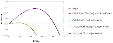
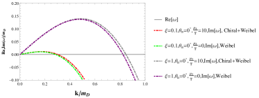
Figure 1: Shows plots of real and imaginary part of the transverse dispersion relation for the case when the angle $\theta_{n}$ between the propagation vector ${\bf k}$ of the perturbation and the anisotropy direction is zero. The modes are purely imaginary and the real part of frequency $\omega=0$. Fig. (1a) shows comparison between pure Weibel modes ($\mu_{5}$=0) with the cases when both the Weibel and chiral-imbalance instabilities are present when $\mu_{5}/T=$1 and $\xi=$0.1,1 . Fig. (1b) depicts the similar comparison when $\mu_{5}/T=$10. It shows that by increasing $\mu_{5}/T$ the chiral-imbalance instability become stronger.

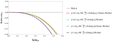
Figure 2: Shows plots of the dispersion relation when $\theta_{n}=\pi/2$. The pure Weibel modes are known to give damping when $\theta_{n}=\pi/2$. For the instances when both the chiral-imbalance and Weibel instabilities are present ( $\mu_{5}/T=$10 and $\xi=$ 0.1,1) the damping can become weaker.

It is important to notice that there also exists a situation $\xi>>1$ when the chiral-imbalance instability can play a dominant role in anisotropic plasma. This is because the Weibel instability growth rate is dependent on $\theta_{n}$ and it is possible to find a particular value of $\theta_{n}=\theta_{nc}$ when the growth rate of the pure-Weibel mode is close to zero. By setting $\omega=0$ in the pure Weibel dispersion relation, one can find for $\xi>>1$, $\theta_{nc}\sim\left(\frac{\pi m_{D}^{2}}{2k^{2}}\right)^{1/2}\frac{1}{\xi^{1/4}}$. In the regime $\xi<1$ but closer to unity at $\theta_{n}=0$, a comparison between the growth rates of the chiral-imbalance ($\Gamma_{ch}$) and Weibel ($\Gamma_{w}$) instabilities is given in the following table:

$\xi$	0.6	0.7	0.8	0.9
$\frac{\Gamma_{ch}}{\Gamma_{w}}$	$\frac{0.0088\alpha_{e}^{3/2}\mu_{5}^{3}}{T^{3}}$	$\frac{0.0076\alpha_{e}^{3/2}\mu_{5}^{3}}{T^{3}}$	$\frac{0.0067\alpha_{e}^{3/2}\mu_{5}^{3}}{T^{3}}$	$\frac{0.0060\alpha_{e}^{3/2}\mu_{5}^{3}}{T^{3}}$

Thus the ratio $\frac{\Gamma_{ch}}{\Gamma_{w}}$ decreases by increasing values $\xi$ while keeping $\mu_{5}/T$ fixed. This is because $\Gamma_{w}$ is increases by increasing $\xi$. For $\alpha_{e}=\frac{1}{137}$ and $\mu_{5}/T\leq 1$ one can clearly see from the table that the ratio $\frac{\Gamma_{ch}}{\Gamma_{w}}\ll 1$. Thus Weibel modes dominates in this case. However when $\mu_{5}/T\gg 1$ chiral modes can also dominate.

Now we consider the case $\xi\ll 1$. This approximation is valid when the initial momentum anisotropy is weak or the Weibel instability has already nearly thermalized (or isotropized) the plasma. This may not be an unlikely scenario in the heavy-ion collisions as the growth rates for the Weibel instabilities can be much larger than the chiral instability. In this case it is possible to evaluate all the integrals in the dispersion relation analytically and one can express $\alpha$, $\beta$, $\gamma$, $\delta$, $\lambda$ and $\chi$ up to linear order in $\xi$ as follows,

$$\alpha=\Pi_{T}+\xi\Big{[}\frac{z^{2}}{12}(3+5\cos{2\theta_{n}})m^{2}_{D}-\frac{1}{6}(1+\cos{2\theta_{n}})m^{2}_{D}$$

$$~{}~{}~{}~{}+\frac{1}{4}\Pi_{T}\left((1+3\cos{2\theta_{n}})-z^{2}(3+5\cos 2\theta_{n})\right)\Big{]};$$

$$z^{-2}\beta=\Pi_{L}+\xi\Big{[}\frac{1}{6}(1+3\cos{2\theta_{n}})m^{2}_{D}+\Pi_{L}\Big{(}\cos{2\theta_{n}}-$$

$$\frac{z^{2}}{2}(1+3\cos{2\theta_{n}})\Big{)}\Big{]};$$

$$\gamma=\frac{\xi}{3}(3\Pi_{T}-m^{2}_{D})(z^{2}-1)\sin^{2}{\theta_{n}};$$

$$\delta=\frac{\xi}{3k}(4z^{2}m^{2}_{D}+3\Pi_{T}(1-4z^{2}))\cos{\theta_{n}};$$

$$\lambda=-\frac{\mu_{5}ke^{2}}{4\pi^{2}}\Big{[}(1-z^{2})\frac{\Pi_{L}}{m^{2}_{D}}\Big{]}-\xi\frac{\mu_{5}ke^{2}}{32\pi^{2}}\Bigg{[}(1-z^{2})\frac{\Pi_{L}}{m^{2}_{D}}\times$$

$$\left((1+7\cos{2\theta_{n}})-3z^{2}(1+3\cos{2\theta_{n}})\right)$$

$$+\frac{1}{3}(1+11\cos{2\theta_{n}})-z^{2}(3+5\cos{2\theta_{n}})\Bigg{]};$$

$$\chi=\xi\left[f(\omega,k)\right],~{}~{}~{}~{}~{}$$ (19)

where $z=\frac{\omega}{k}$ and $f(\omega,k)$ is some function $k$ and $\omega$. But in the present analysis exact form of $f(\omega,k)$ may not be required. Using the above equations and Eqs. (16, 17) one can finally express Eq.(18) in terms of $k$ and $\omega$. One can notice from Eq.(19) that the most significant contribution for $\gamma$, $\delta$, $\lambda$ and $\chi$ is $O(\xi)$. Thus in the present scheme of approximation one can write Eq.(18) up to $O(\xi)$ as:

$$C^{2}_{A}C_{L}-C_{T}C_{L}(C_{n}+C_{T})=0,$$ (20)

which in turn can give following two branches of the dispersion relation,

$$C^{2}_{A}-C^{2}_{T}-C_{n}C_{T}=0,$$ (21)

$$C_{L}=0.$$ (22)

First, we would like to note that when $C_{A}=0$, Eqs.(21-22) reduces to exactly the same dispersion relation discussed in Ref.[41] for the Weibel instability in an anisotropic plasma when there is no parity violating effect. Let us consider Eq.(21), it can be written as:

$$(k^{2}-\omega^{2})^{2}+(k^{2}-\omega^{2})(2\alpha+\gamma)+\alpha^{2}+\alpha\gamma-\lambda^{2}=0.$$ (23)

This equation is a quadratic equation in $(k^{2}-\omega^{2})$ and it’s solutions can be written as,

$$(k^{2}-\omega^{2})=\frac{-(2\alpha+\gamma)\pm 2\lambda}{2}.$$ (24)

Now, it is of particular interest to consider the quasi-static limit $\left|{\omega}\right|<<k$, in this limit expressions for $\alpha\sim\Pi_{T}$ and $\beta\sim\frac{\omega^{2}}{k^{2}}\Pi_{L}$ and $\lambda\sim-\frac{\Pi_{A}}{2}$. Now $\Pi_{L}$, $\Pi_{T}$ and $\Pi_{A}$ can be obtained by expanding Eq.(17) in the quasi static limit as:

$${\Pi_{T}}_{\arrowvert_{\left|{\omega}\right|<<k}}=\left(\mp{i}\frac{\pi}{4}\frac{\omega}{k}\right)m^{2}_{D};$$

$${\Pi_{L}}_{\arrowvert_{\left|{\omega}\right|<<k}}=m^{2}_{D}\left[\mp{i}\frac{\pi}{2}\frac{\omega}{k}-1\right]$$

$${\Pi_{A}}_{\arrowvert_{\left|{\omega}\right|<<k}}=\frac{\mu_{5}ke^{2}}{2\pi^{2}}\left(\frac{{\Pi_{L}}_{\arrowvert_{\left|{\omega}\right|<<k}}}{m^{2}_{D}}\right)$$ (25)

Thus in the quasi-stationary limit one can write positive branch of the transverse modes given by Eq.(24) as:

$$\rho(k)=\frac{\left(\frac{4\alpha_{e}\mu_{5}}{\pi^{2}m^{2}_{D}}\right)k^{2}\left[1-\frac{\pi k}{\mu_{5}\alpha_{e}}+\frac{\xi\left(1+5\cos{2\theta_{n}}\right)}{12}+\frac{\xi\left(1+3\cos{2\theta_{n}}\right)}{12}\frac{\pi m^{2}_{D}}{\mu_{5}\alpha_{e}k}\right]}{{\left[1+\frac{2\mu_{5}\alpha_{e}k}{\pi m^{2}_{D}}(1-\frac{\xi}{4})+\xi\cos{2\theta_{n}}\left(1-\frac{7\mu_{5}\alpha_{e}k}{2\pi m^{2}_{D}}\right)\right]}}$$ (26)

Here we have used $\omega=i\rho(k)$ and defined $\alpha_{e}=\frac{e^{2}}{4\pi}$ as the electromagnetic coupling. It is clear from Eq.(26) that $\omega$ is purely an imaginary number and its real-part is zero i.e. $Re(\omega)=0$. Positive $\rho(k)>0$ implies an instability as $e^{-i(i\rho(k))t}\sim e^{+\rho(k)t}$. From Eq.(26), in the limit $\xi\rightarrow 0$ and $\mu_{5}\rightarrow 0$ one gets $\rho(k)=-\frac{4k^{3}}{\pi m^{2}_{D}}$. Thus for an isotropic plasma (of massless particles) without any chiral-imbalance there is no unstable propagating mode when $\omega\ll k$. Which is consistent with fact that without any source of free energy there should not be any unstable mode.

Now let us first consider that the quasi-static limit $|\omega|<<k$ indeed satisfies for Eq.(26). Since we have already assumed that $\xi<<1$ and $\alpha_{e}<1$ and for $\mu_{5}<<T$ one can have $\frac{\mu_{5}}{m_{D}}\approx\frac{1}{2\alpha_{e}^{1/2}}\left(\frac{\mu_{5}}{T}\right)$. From this it is rather easy to show that $\rho/k<<1$ if the condition $\frac{k^{2}}{m_{D}^{2}}<<1$ is satisfied. In this case denominator of Eq.(26) can be approximated to unity. Now we write the above equation as:

$$\rho(k)=\frac{4}{\pi}\frac{k^{2}}{m^{2}_{D}}\Bigg{[}\frac{\alpha_{e}\mu_{5}}{\pi}-k+\frac{\alpha_{e}\xi\mu_{5}}{12\pi}\left(1+5\cos{2\theta_{n}}\right)+$$

$$\frac{\xi}{12}\frac{m^{2}_{D}}{k}\left(1+3\cos{2\theta_{n}}\right)\Bigg{]}.$$ (27)

Here we emphasize that when $\xi=0$, first two terms in the square bracket survives and Eq.(27) matches with the dispersion relation of the chiral instability given in Ref.[30] and when $\mu_{5}=0$, the second and the last term survives to give the Weibel modes considered in Ref.[41]. Term with $\alpha_{e}\xi\mu_{5}$ factor arises due to the interaction between the Weibel and chiral-imbalance modes.

Before we analyse the interplay between the chiral-imbalance and the Weibel instabilities, it is instructive to qualitatively understand their origin. First consider the chiral-imbalance instability. For a such a plasma ‘chiral-charge’ density $n$ is given by $\partial_{t}n+{\bf\nabla\cdot j}=\frac{2\alpha_{e}}{\pi}{\bf E\cdot B}$. From this one can estimate the axial charge density $n\sim\alpha_{e}kA^{2}$ where $A$ is the gauge-field. Assuming that there are only right handed particles i.e ($\mu_{5}\sim\mu_{R}$) then the number and energy densities of the plasma respectively given by $\mu_{5}T^{2}$ and ${\mu_{5}}^{2}T^{2}$. The fermionic number density associated with the gauge field can be estimated from the Chern-Simon term to be $\alpha_{e}kA^{2}$. The number densities associated with the fields and particles have same value for $k_{1}\sim\frac{\mu_{5}T^{2}}{\alpha_{e}A^{2}}$. The typical energy for the gauge field $\epsilon_{A}\sim k^{2}A^{2}$. For this particular value of $k_{1}$ it can be seen that $\epsilon_{A}={\mu_{5}}^{2}T^{2}\frac{T^{2}}{\alpha_{e}^{2}A^{2}}$. Thus there exists a state satisfying the condition $\frac{T^{2}}{\alpha_{e}^{2}}<A^{2}$ for which energy in the gauge field is lower than particle energy. This leads to the chiral-imbalance instability[30, 34]. The Weibel instability arises when the equilibrium distribution function of the plasma has anisotropy in the momentum space[44, 45]. The anisotropy in the momentum space can be regarded as anisotropy in temperature. Suppose there is plasma which is hotter in $y$-direction than $x$ or $z$ direction one may write the distribution function $n^{0}_{p}=\frac{1}{1+e^{-(\sqrt{p^{2}_{x}+(1+\xi)p^{2}_{y}+p^{2}_{z}})/T}}$ . If in this situation a disturbance with a magnetic-field $B=B_{0}cos(kx)$ which arises say from noise, one can write the Lorentz force term in the kinetic equation as $e(v\times B)\cdot\partial_{p}n^{0}_{p}=e[\xi(v_{z}B_{x}-v_{x}B_{z})\frac{p_{y}}{T}]\left(\frac{-e^{-(\sqrt{p^{2}_{x}+(1+\xi)p^{2}_{y}+p^{2}_{z}})/T}}{1+e^{-(\sqrt{p^{2}_{x}+(1+\xi)p^{2}_{y}+p^{2}_{z}})/T}}\right)$. This Lorentz-force can produce current-sheets where the magnetic field changes its sign. The current-sheet in turn enhance the original magnetic field [44, 45].

The Weibel instability is known to grow maximally for $\theta_{n}=0$. In the quasi-static limit the instability has maximum growth rate $\Gamma_{w}\sim\frac{8\xi^{3/2}}{27\pi}m_{D}$ for $k=\frac{\sqrt{\xi}}{3}m_{D}$. For the chiral imbalance instability the maximum growth rates $\Gamma_{ch}\sim\frac{16\alpha_{e}^{3}}{27\pi^{4}}\left(\frac{\mu_{5}}{m_{D}}\right)^{2}\mu_{5}$, occurs at $k\sim\frac{2\alpha_{e}}{3\pi}\mu_{5}$[30]. Thus the ratio $\frac{\Gamma_{ch}}{\Gamma_{w}}\sim\frac{2}{\pi^{3}}\left(\frac{\alpha_{e}}{\xi^{1/2}}\right)^{3}\left(\frac{\mu_{5}}{m_{D}}\right)^{3}$ $\sim\frac{1}{4\pi^{3}}\left(\frac{\alpha_{e}}{\xi}\right)^{3/2}\left(\frac{\mu_{5}}{T}\right)^{3}$, where we have used $\frac{\mu_{5}}{m_{D}}\approx\frac{1}{2\alpha_{e}^{1/2}}\left(\frac{\mu_{5}}{T}\right)$. The ratio $\frac{\Gamma_{ch}}{\Gamma_{w}}$ becomes unity when $\xi_{c}\approx 2^{2/3}\left(\frac{\alpha_{e}}{4\pi^{2}}\right)\left(\frac{\mu_{5}}{T}\right)^{2}$. When $\mu_{5}\sim T$ and $\alpha_{e}=1/137$ (QED) one can estimate $\xi_{c}<10^{-3}$. $\xi_{c}$ will change if coupling varries (QCD case). Thus for $\xi_{c}<\xi<<1$ the Weibel instability can dominates over the chiral imbalance modes. However, it may be still possible to see the chiral-imbalance modes if we consider $\theta_{n}-$dependence of the instability described by Eq.(27). In Eq.(27) the Weibel instability term vanishes if $\theta_{n}\sim\frac{1}{2}\cos^{-1}(1/3)\sim 55^{\circ}$. For this value of $\theta_{n}$ the interaction term between the Weibel and the chiral modes becomes negative and tries to suppress the unstable mode. However this term is very small in comparison to the pure chiral term.

In figure (3) we plot the dispersion relation given by Eq.(26) as function of $k_{N}=\frac{\pi}{\alpha_{e}\mu_{5}}k$ for various values of $\xi$ which is given in units of $\xi_{c}$ and the propagation angle $\theta_{n}$. $y$-axis shows the $Re[\omega]$ and $Im[\omega]/\left(\frac{4\alpha_{e}^{3}{\mu_{5}}^{3}}{\pi^{4}m^{2}_{D}}\right)$. Note that the real part of the frequency $Re[\omega]$ is zero For the case when $\xi=0$ there is no Weibel mode and the only the chiral-imbalance can give the instability. Whereas when $\mu_{5}=0$ only Weibel instability will contribute. From the condition $\rho(k)>0$, one can obtain the range of the instability which can be stated as:

$$k_{N}=1+\frac{\xi\left(1+cos2\theta_{n}\right)}{12}+\Bigg{[}\left(1+\frac{\xi\left(1+cos2\theta_{n}\right)}{12}\right)^{2}+\frac{\pi^{2}\xi\left(1+3cos2\theta_{n}\right)}{3\alpha_{e}}\Bigg{]}^{1/2}$$ (28)

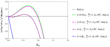
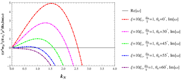
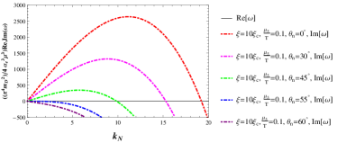
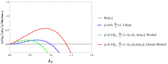
Figure 3: Shows plots of real and imaginary part of the dispersion relation. Here $\theta_{n}$ is the angle between the wave vector $k$ and the anisotropy vector. Real part of dispersion relation is zero. Fig. (3a) show plots for three cases: (i) Pure chiral (no anisotropy), (ii) Pure Weibel (chiral chemical potential=0) and (iii) When both chiral and Weibel instabilities are present. Fig. (3b-3d) represent the case when both the instabilities are present but the anisotropy parameter varies at different values of $\theta_{n}$ for fixed $\mu_{5}/T=1$. Fig. (3e-3f) represents the case when both instabilities are present for a fixed anisotropy parameter at different values of $\theta_{n}$ when $\mu_{5}/T=1$ and $\mu_{5}/T=0.1$ respectively. Fig. (3g) represents the case when for a particular value of $\theta_{n}\sim\theta_{c}$ both the instabilities have equal growth rates. Here frequency is normalized in unit of $\omega/\left(\frac{4\alpha_{e}^{3}{\mu_{5}}^{3}}{\pi^{4}m^{2}_{D}}\right)$ and wave-number $k$ by $k_{N}=\frac{\pi}{\mu_{5}\alpha_{e}}k$.

In Fig.(3a) we have shown for $\theta_{n}=0$ the pure Weibel case ($\xi=10\xi_{c}$ and $\mu_{5}=0$) and the pure chiral-case ($\xi=0$ and $\mu_{5}\neq 0$) with the case when both the instabilities are present i.e. $\xi=10\xi_{c}$ and $\mu_{5}\neq 0$. The plot shows that the pure Weibel modes dominating over the pure chiral case. But the combined effect of both the instabilities is much more pronounced. The maximum growth rate and the range of the instability are altered significantly for the combined case. In Figs. (3b-3d) we study the cases where both the instabilities are present and $\xi$ and $\theta_{n}$ vary when $\mu_{5}/T=1$. It is important to note that in this analysis we are showing the plots of the dispersion relation following the same normazation as used in Ref.[30] so that we can compare our results. Due to the normalization rescaling of dispersion relation for Weibel term picks up factor $\mu_{5}/T$ and therefore apart from $\xi$ and $\theta_{n}$ Weibel instability also becomes dependent on $\mu_{5}/T$. However, in order to take limit $\mu_{5}\rightarrow 0$ one need to unscale normalized $Im[\omega]$ and $k_{N}$ in terms of $Im[\omega]$ and $k$. Fig.(3b) shows clearly shows for $\theta_{n}=0$ when condition $\xi<<\xi_{c}$ is satisfied, the chiral instability dominates over the Weibel modes. However, such values of $\xi$ are extremely small. For the cases when $\xi\geq\xi_{c}$ the Weibel modes are dominating. Contribution from the Weibel modes is maximum for $\theta_{n}=0$ and the modes are strongly damped at $\theta_{n}=\pi/2$. Angular part in the dispersion relation for the pure Weibel modes becomes zero when $\theta_{n}\approx 55^{0}$. In this case one can see that chiral modes can remain dominant. This case is shown in Fig.(3c). It should be noted that for the case when $\xi>>\xi_{c}$ the contribution from the coupling term between the Weibel and chiral modes become sufficiently strong and it can again suppress the instability. In Fig.(3d) we have shown the case when $\theta_{n}=\pi/2$. The modes with $\xi\geq\xi_{c}$ are strongly damped and there is no instability. Here the coupling term between the two modes also contribute in the damping of the instability. In Fig.(3e-3f) we have plotted the unstable modes for $\xi=10\xi_{c}$ for different values of $\theta_{n}$ when $\mu_{5}/T=1$ and $0.1$ respectively. In this case see when $\mu_{5}/T=0.1$ i.e. ($\mu_{5}<<T$) the instability increases enormously. Now by comparing the growth rates of pure-Weibel and pure chiral modes, when $\mu_{5}/T=1$, one can find that they become equal at $\theta_{c}=\frac{1}{2}\cos^{-1}\left[\left(\frac{2}{27}\right)^{2/3}\frac{3\alpha_{e}}{\xi\pi^{2}}-\frac{1}{3}\right]$. Fig.(3g) represents this case where we have shown that the growth rate of pure Weibel case at $\xi=0.15\xi_{c}$ becomes comparable to pure chiral mode with $\xi=0$. The topmost (red) curve in this figure shows the case when both the modes operate together. This case shows that the combined effect of the instability can significantly alter the range and the growth rate of the instability.

In conclusion, we have studied collective modes in an anisotropic chiral plasma where the both Weibel and chiral-imbalance instabilities are present. We have demonstrated that for $\theta_{n}=0$, only for a very small values of the anisotropic parameter $\xi\sim\xi_{c}\ll 1$ growth rates of the both instabilities are comparable. For the cases when $\xi\geq 1$, $\xi<1$ but closer to unity and $\xi_{c}<\xi\ll 1$, the Weibel modes dominate over the chiral-imbalance instability. We have also shown for the case when $\xi\gg 1$, the chiral-imbalance can dominate over the Weibel modes for certain values of $\theta_{n}$.

Acknowledgements: The authors would like to thank the anonymous referees for their constructive comments and suggestions.

References

[1]
L. D. Landau and E. M. Lifshitz, Physical Kinetics
(Pergamon, New York, 1981).
[2]
D. T. Son and P. Surowka,
Phys. Rev. Lett. 103, 191601 (2009) [arXiv:0906.5044 [hep-th]].
[3]
N. Banerjee, J. Bhattacharya, S. Bhattacharyya, S. Jain, S. Minwalla, and T. Sharma,
JHEP 1209, 046 (2012)
[arXiv:1203.3544 [hep-th]].
[4]
K. Jensen,
Phys. Rev. D 85, 125017 (2012)
[arXiv:1203.3599 [hep-th]].
[5]
D. E. Kharzeev and D. T. Son,
Phys. Rev. Lett. 106, 062301 (2011). [arXiv:1010.0038 [hep-ph]].
[6]
D. T. Son and N. Yamamoto,
Phys. Rev. Lett. 109, 181602 (2012).
[arXiv:1203.2697 [cond-mat.mes-hall]].
[7]
I. Zahed, Phys. Rev. Lett. 109, 091603 (2012).
[8]
M. A. Stephanov and Y. yin, Phys. Rev. Lett. 109, 162001 (2012).
arXiv:1207.0747[hep-th]
[9]
Jiunn-Wei Chen, Shi Pu, Qun Wang and Xin-Nian Wang, Phys. Rev. Lett. 110, 262301 (2013).
[10]
R. Loganayagam and P. Surowka, J. High Energy Phs. 04, 079 (2012).
arXiv:1201.2812[hep-th]
[11]
D. Xiao, J. Shi and Q. Niu, Phys. Rev. Lett. 95, 137204 (2005).
[12]
M. V. Berry, Proc. R. Soc. Lond. A 392, 45 (1984)
[13]
S. Adler, Phys. Rev. 177, 2426 (1969).
[14]
J.S. Bell and R. Jackiw, Nuovo Cimento A 60 4 (1969).
[15]
H. B. Nielsen and M. Ninomiya,
Phys. Lett. B 130, 389 (1983).
[16]
A. Vilenkin, Phys. Rev. D 22, 3080 (1980).
[17]
K. Fukushima, D. E. Kharzeev, and H. J. Warringa,
Phys. Rev. D 78, 074033 (2008).
[18]
D. E. Kharzeev, L. D. McLerran and H. J. Warringa, Nucl. Phys. A 803, 67 92007).
[19]
H. J. Warringa, arXiv:0805.1384[hep-ph].
[20]
B. I. Abelev et. al. [STAR Collaboration], Phys. Rev. Lett. 103, 251601 (2009).
arXiv:0909.1739 [nucl-ex]
[21]
B. I. Abelev et. al. [STAR Collaboration], Phys. Rev. C. 81, 054908 (2010).
arXiv:0909.1717[nucl-ex].
[22]
D. Xiao, M.-C. Chang, and Q. Niu,
Rev. Mod. Phys. 82, 1959 (2010).
[arXiv:0907.2021 [cond-mat.mes-hall]].
[23]
Heon-Jung Kim et. al., Phys. Rev. Lett. 111, 246603 (2013).
[24]
K. Sasaki, arXiv:0106190 [cond-mat].
[25]
D. T. Son and N. Yamamoto,
Phys. Rev. D 87, 085016 (2013) [arxiv:1210.815].
[26]
C. Manuel and J. M. Torres-Rincon, arXiv:1312.1158[hep-ph].
[27]
H. Itoyama and A. H. Mueller, Nucl. Phys. B, 165, 349 (1983).
[28]
Y. Li and G. Ni, Phys. Rev. D. 38, 3840 (1988).
[29]
A. Gomez Nicola and R. F. Alvarez-Estrada, Int. J. Mod. Phys. A 9, 1423 (1994).
[30]
Y. Akamatsu and N. Yamamoto, Phys. Rev. Lett. 111, 052002 (2013).
[31]
J. F. Nieves and P. B. Pal, Phys. Rev. D 39, 652 (1989).
[32] A. N. Redlich and L. C. R. Wijewardhana,
Phys. Rev. Lett. 54, 970 (1985).
[33]
V. A. Rubakov,
Prog. Theor. Phys. 75, 366 (1986).
[34]
M. Joyce and M. E. Shaposhnikov,
Phys. Rev. Lett. 79, 1193 (1997).
[35]
M. Laine,
JHEP 0510, 056 (2005).
[36]
A. Boyarsky, J. Frohlich, and O. Ruchayskiy,
Phys. Rev. Lett. 108, 031301 (2012).
[37]
S. Mrówczynski, Phys. Lett. B 214, 587 (1988),
S. Mrówczynski, Phys. Lett. B 314, 118 (1993), J. Randrup and S.Mrówczynski,
arXiv:0303021[nucl-th].
[38]
J. R. Bhatt, P. K. Kaw and J. C. Parikh, Pramana- J. Phys. 43, 467 (1994)
[39]
P. A. Arnold, J. Lenaghan and G. D. Moore, J. High Energy Phs. 08, 002 (2003).
[40]
P. Romatschke and R. Venugopalan, Phys. Rev. Lett. 96, 062302 (2006)
[41]
Paul Romatschke and Michael Strickland, Phys. Rev. D 68, 036004 (2003).
[42]
L. N. Tsintsadze, Phys. Plasmas, 16, 094507 (2009).
[43]
B. Y. Hu and J. W. Wilkins, Phys. Rev. B 43, 14 009 (1991).
[44]
E.S. Weibel, Phys. Rev. Lett. 2, 83 (1959).
[45]
B.D. Fried, Phys. Fluids 2, 337 (1959).
[46]
N. A. Krall and A. W. Trivelpiece, Principles of Plasma Physics(San Francisco Press, San Francisco, 1986).
[47]
R. Kobes, G. Kunstatter and A. Rebhan, Nucl. phys. B, 355 1 (1991).