CoCos under short-term uncertainty

Abstract

In this paper we analyze an extension of the Jeanblanc and Valchev [12] model by considering a short-term uncertainty model with two noises. It is a combination of the ideas of Duffie and Lando [9] and Jeanblanc and Valchev [12]: share quotations of the firm are available at the financial market, and these can be seen as noisy information about the fundamental value, or the firm’s asset, from which a low level produces the credit event. We assume there are also reports of the firm, release times, where this short-term uncertainty disappears. This credit event model is used to describe conversion and default in a CoCo bond.

JEL Classification: G11 G12 G13 G18 G21 G32

1 Introduction

A contingent convertible (CoCo) is a bond issued by a financial institution such that, upon the appearance of a credit event, an automatic conversion into a predetermined number of shares takes place. This credit event is related to a possible distress period of the institution, and thus the conversion intends to be a loss absorbing security, in the sense that in case of liquidity difficulties it produces a recapitalization of the entity. An alternative to the bond conversion into shares is to force a partial write-down of the bond’s face value. We shall however only consider the first type of conversion here.

There is disagreement about how to establish the trigger or credit event. It is perhaps the most controversial issue in a CoCo. Some advocate conversion based on book values, such as the different capital ratios used in Basel III. Others defend market triggers such as the market value of the equity. So far the CoCos issued by the private sector are based on accounting ratios.

From a modelling point of view, and depending on the trigger chosen for the conversion, one can follow different approaches: a structural approach which links conversion to a low level of a certain index related to the firm’s asset, debt or equity; or a reduced-form approach assuming a conversion intensity that can depend on certain explicative factors. This latter approach is specially useful when pricing CoCos is the main interest, it is a kind of statistical modelling of the conversion trigger. In fact what one models is the law of the conversion time. On the other hand, from the structural approach for modelling the trigger one models the random variable describing the conversion time, and one relates it to the dynamics of the firm’s assets, debt, or equities. It is a more explanatory approach where one can use the observed dynamics of certain economics facts in order to explain the conversion time.

Conversion is a kind of credit event which is similar to default and empirical facts show that such events happen all of a sudden, in such a way that bond prices drop precipitously in a way not completely expected. This behavior, that is compatible with the existence of an intensity for the credit event, is observed from the fact that yield spreads are strictly positive at zero maturity. Structural models where the default is linked to the first time that a diffusion process falls below a certain level do not reproduce this behavior. Their corresponding default times are predictable, the yield spreads go to zero when the time to maturity goes to zero, they are models with zero intensity. Of course, we can consider a jump-diffusion but then there is not much difference when modelling the jumps of the diffusion from modelling the intensity, see, for instance, Zhou [21]. Another way of explaining the inaccessibility of the default time is that the information about the process involved in the default or conversion is not perfect, maybe because the firm’s assets are not observable, or they are observable only at certain times, maybe because there is certain delay or noise in the accounting reports, etc. Note that this is in fact the most sensible and explanatory way of modelling the credit events. Credit events have their own reasons linked to the economic behavior of the firm or one sector, but at the same time only experts or managers are aware about the current behavior of the firm or sector and market participants have only noisy or delayed information. As a result the model, being structural from the point of view of managers becomes a reduce form model from the market view. A precedent for this approach is Duffie and Lando [9] who is the first serious attempt to study the consequences of noisy information in structural models. Another precedent is Jarrow et al. [20], where the market information is a reduction of the manager’s information, in particular they assume that a credit event happens after a long negative cash balance situation followed by a drop that duplicates the bad cash balance, however market only sees the sign of cash balances and the time of default. This latter model is certainly a very particular one that takes advantage of the behavior of Brownian excursions but its extension, though appealing, is, as far as we know, an open problem. Finally the third important reference is Jeanblanc and Valchev [12] where they discuss the effect of different types of partial information, allowing some update times at which the information becomes complete. This motivates the idea of what we call a short-term uncertainty model, that is, a model where the uncertainty in the observation is only present in between update times.

In this paper we analyze an extension of the Jeanblanc and Valchev [12] model by considering a short-term uncertainty model with two noises. It is a combination of the ideas of Duffie and Lando [9] and Jeanblanc and Valchev [12]: share quotations of the firm are available at the financial market, and these can be seen as noisy information about the fundamental value, or the firm’s asset, from which a low level produces the credit event. We assume there are also reports of the firm, release times, where this short-term uncertainty disappears. This credit event model is used to describe conversion and default in a CoCo bond.

2 Pricing CoCos

Every pricing model for a CoCo starts by defining the mechanisms that trigger default and conversion. From a structural modelling approach we can say, in general terms, that CoCo’s conversion and the issuer’s ulterior default are triggered as soon as a fundamental process $(U_{t})_{t\geq 0}$ crosses, respectively, the levels $\bar{c}$ and $\underline{c}$ , i.e.,

$$\tau=\inf\{t\geq 0\;:\;U_{t}\leq\bar{c}\}\qquad\text{and}\qquad\delta=\inf\{t\geq 0\;:\;U_{t}\leq\underline{c}\}.$$ (1)

The subsequent difference between models relies on how this fundamental process is defined in order to serve as proxy for the regulatory capital, and how the correspondent prices are evaluated. A prominent particular choice for $(U_{t})_{t\geq 0}$ is the given by

$$U_{t}:=\log\frac{S_{t}}{\ell_{t}},\qquad t\geq 0,$$ (2)

where $(S_{t})_{t\geq 0}$ stands for the issuer’s share price, and $(\ell_{t})_{t\geq 0}$ models the main benchmark for the issuer performance. The importance of this process has been already addressed in earlier literature on credit risk as in Longstaff and Schwarz [14] and Saá-Raquejo and Santa-Clara [19]. The process in (2) is also referred to as log-leverage or solvency ratio process. We use the term fundamental since all credit events are assumed to be triggered by the movements of $(U_{t})_{t\geq 0}$ to a series of critical barriers. Furthermore, the correspondent pricing formulas will be obtained in terms of $(U_{t})_{t\geq 0}$, not in terms of $(S_{t})_{t\geq 0}$ and $(\ell_{t})_{t\geq 0}$ independently.

Traditionally, structural models operate under two important but arguable assumptions:

$(\mathbf{A}_{1})$

The correlation between the noises driving the share price and $(U_{t})_{t\geq 0}$ is constant.

$(\mathbf{A}_{2})$

The fundamental process is fully observable in continuous time.

However, in practice, it seems more reasonable to assume that this is not the case, and assume instead the presence of a short-term uncertainty in the following sense:

$(\mathbf{A}^{\prime}_{1})$

The correlation between the noises driving the share price and $(U_{t})_{t\geq 0}$ may vary.

$(\mathbf{A}^{\prime}_{2})$

The fundamental process is fully observable only at predetermined dates $(T_{j})_{t\in\mathbb{Z}_{+}}$.

Notice that, in some sense, the assumption $(\mathbf{A}^{\prime}_{2})$ accounts for the fact that in most cases regulatory capital depends on the balance sheets of the firm issuing the CoCo, and those sheets are updated only at series of predetermined dates $(T_{j})_{t\in\mathbb{Z}_{+}}$. On the other hand, it seems more natural to assume $(\mathbf{A}^{\prime}_{1})$ and include the correlation $\rho$ between the share price and the fundamental process as another rightful model parameter. From now on we shall exclude the case where we have a perfect correlation between the stock and the fundamental process, i.e., the case where $\rho=1$.

Working under the short-term uncertainty has two immediate consequences. On the one hand, and deviating from other structural models, the assumption $(\mathbf{A}^{\prime}_{1})$ prevents default and conversion times from being stopping times with respect to the filtration generated by the relevant state variables (e.g., share price, interest rates, total assets value,…). On the other hand, assumption $(\mathbf{A}^{\prime}_{2})$ implies an information structure which is different from other partial information models as Coculescu et al. [6], Collin-Dufresne et al. [7], Duffie and Lando [9], and Gou et al. [10]. The work of Jeanblanc and Valchev [12] is closer to our model and, as mentioned in the introduction, this work combines techniques of [9] and [12], giving in some sense a two variate extension of [12].

3 Short-term uncertainty

3.1 Introducing assumption ($\mathbf{A}_{1}^{\prime}$).

We shall assume that the $n$-dimensional $\mathbb{P}^{*}$-Brownian motion $(W_{t}^{*}:=(W_{1,t}^{*},...,W_{n,t}^{*}))_{t\geq 0}$ is the noise driving all relevant state variables (e.g., share price, interest rates, total assets value,…). In particular, we shall assume that the $\mathbb{P}^{*}$-dynamics of the share price $(S_{t})_{t\geq 0}$ be given by

$$\frac{\mathrm{d}S_{t}}{S_{t}}=r_{t}\mathrm{d}t+\sigma_{t}\cdot\mathrm{d}W_{t}^{*},$$ (3)

where we have used $(r_{t})_{t\geq 0}$ to denote the interest rate, and the $(\sigma_{t})_{t\geq 0}$ is positive $\mathbb{R}^{n}$-valued càdlàg process, integrable with respect to $(W_{t}^{*})_{t\geq 0}$. Hereafter the symbol $\cdot$ denotes the dot product in $\mathbb{R}^{n}$.

Additionally, given a correlation function $\rho:\mathbb{R}_{+}\rightarrow[-1,1]$, let $(W_{t}^{\rho}:=(W_{j,t}^{\rho},...,W_{n,t}^{\rho}))_{t\geq 0}$ be a second $\mathbb{P}^{*}$-Brownian motion satisfying $\mathrm{d}W_{j,t}^{*}\mathrm{d}W_{j,t}^{\rho}=\rho_{j}(t)\mathrm{d}t$. In these terms, we consider the parametric family

$$\mathrm{d}U_{t}=\mu_{t}\mathrm{d}t+\sigma^{\prime}_{t}\cdot\mathrm{d}W_{t}^{\rho},$$ (4)

where $(\sigma^{\prime}_{t})_{t\geq 0}$ is positive $\mathbb{R}^{n}$-valued càdlàg process, integrable with respect to $(W_{t}^{\rho})_{t\geq 0}$. Let us note that at this point we don’t assume any specific model for volatilities $(\sigma_{t})_{t\geq 0}$ and $(\sigma^{\prime}_{t})_{t\geq 0}$.

We shall further assume that all credit events are triggered by the movements of $(U_{t})_{t\geq 0}$ to a series of critical barriers. More specifically, the conversion and default times will be given respectively by

$$\tau=\inf\{t\geq 0\;:\;U_{t}\leq\bar{c}\}\qquad\text{and}\qquad\delta=\inf\{t\geq 0\;:\;U_{t}\leq\underline{c}\},$$ (5)

For simplicity in the exposition we shall assume that no coupons are attached to the CoCo. However, we remark that the coupon cancellation feature introduced in [8] can be included in a natural way by establishing that the $j$-th coupon will be paid at time $T_{c_{j}}$ if and only if the $\tau_{j}(\rho)>T_{c_{j}}$ where

$$\tau_{j}:=\inf\{t\geq 0\;:\;U_{t}\leq\bar{c}_{j}\},\qquad j=1,...,m.$$ (6)

It will be assumed that constants are ordered as $\underline{c}<\bar{c}\leq\bar{c}_{m}\leq...\leq\bar{c}_{1}$ so that the coupon cancellation, conversion and default may only occur in a sequenced way.

3.2 Introducing assumption ($\mathbf{A}_{2}^{\prime}$).

Let the set $\{T_{j},\;j\in\mathbb{Z}_{+}\}$ denote the times at which we fully observe $(W_{t}^{\rho})_{t\geq 0}$. In addition, we assume that $(W_{t}^{*})_{t\geq 0}$ is observed at times $\{t_{i,j},\;i=0,...,n,\;j\in\mathbb{Z}_{+}\}$ where we set $T_{0}:=0$ and $t_{i,0}=T_{i}$. Let us define

$$\left\lfloor t\right\rfloor:=\min\{T_{j}\in\{T_{0},T_{1},T_{2},...\}\;:\;T_{j}\leq t<T_{j+1}\},\qquad t\geq T_{0}.$$

Let $\mathbb{F}^{W^{\rho}}=(\mathcal{F}_{t}^{W^{\rho}})_{t\geq 0}$ and $\mathbb{F}^{W^{*}}=(\mathcal{F}_{t}^{W^{*}})_{t\geq 0}$ denote the natural filtration generated by $(W_{t}^{\rho})_{t\geq 0}$ and $(W_{t}^{*})_{t\geq 0}$, respectively. In these terms, our reference information about the two noises $(W_{t}^{*})_{t\geq 0}$ and $(W_{t}^{\rho})_{t\geq 0}$ is given by $\widetilde{\mathbb{F}}=(\widetilde{F}_{t})_{t\geq 0}$ with

$$\widetilde{\mathcal{F}}_{t}:=\mathcal{F}_{\left\lfloor t\right\rfloor}^{W^{\rho}}\vee\sigma(\{W^{*}_{t_{ij}},t_{ij}\leq t\}),\qquad t\geq 0.$$

Notice that $\mathcal{F}_{\left\lfloor t\right\rfloor}^{W^{\rho}}=\mathcal{F}_{t}^{W^{\rho}}$ for every $t\in\{T_{j},\;j\in\mathbb{Z}_{+}\}$, but $\mathcal{F}_{t}^{W^{\rho}}\varsupsetneq\mathcal{F}_{\left\lfloor t\right\rfloor}^{W^{\rho}}$ otherwise. Thus in our model there is a noise which clears out at update times $(T_{j})_{j\in\mathbb{Z}_{+}}$. Further, in between two update times, say $T_{j}$ and $T_{j+1}$, the correlated process $(S_{t})_{t\geq 0}$ provides a noisy information about $(U_{t})_{t\geq 0}$ by means of the observations $\{S_{t_{j,0}},S_{t_{j,1}}...,S_{t_{j,n}}\}$, where $T_{j}=t_{j,0}\leq...\leq t_{j,n}=T_{j+1}$.

As already pointed out in the introduction, there are some differences between our model and other related approaches dealing with incomplete information in the credit risk literature. For instance, Coculescu et al. [6] consider a similar setting in which instead of $(U_{t})_{t\geq 0}$ they only observe a correlated process $(U_{t}^{\rho})_{t\geq 0}$. However, their observation of $(U_{t}^{\rho})_{t\geq 0}$ is continuous, whereas we only fully observe it at times $(T_{j})_{t\in\mathbb{N}}$. Similar arguments apply for [7] and Duffie and Lando [9]. On the other hand, our model also differs from that in Gou et al. [10] since the proposed update at times disrupts the permanent delay in the arrival of information considered in [10].

On the other hand, our model also deviates from traditional structural models since the credit events in (5) and (6) are no longer stopping times with respect to the reference filtration $\widetilde{\mathbb{F}}$. We shall consider the full market information $\mathbb{G}=(\mathcal{G}_{t})_{t\geq 0}$ as given by $\mathcal{G}_{t}:=\widetilde{\mathcal{F}}_{t}\vee\mathcal{H}_{t}$ where $\mathcal{H}_{t}:=\sigma(\textbf{1}_{\{\tau\leq s\}},\;s\leq t)$.

Remark 3.1.

The short-term uncertainty model presented here can be readily stated in a more general way, for instance by replacing $(W_{t}^{*})_{t\geq 0}$ by a more general Lévy process. Since here we are interested to obtain analytical price formulas, we shall not consider the possibility of including jumps in the share price (nor the fundamental process) dynamics. However, we note here that a numerical study in the presence of jumps can be conducted, for instance, using the techniques in Metwally and Atiya[16], Ruf and Scherer [18] or Hieber and Scherer [11].

3.3 Compensator of $\tau$

Define the process $(F(t):=\mathbb{P}^{*}(\tau\leq t|\widetilde{\mathcal{F}}_{t}))_{t\geq 0}$. In a standard structural model, $\tau$ would be a stopping time with respect to the reference filtration $\widetilde{\mathbb{F}}$, leading to the identity $F(t)=\textbf{1}_{\{\tau\leq t\}}$. Under the Assumption $\mathbf{A}_{2}^{\prime}$, however, $\textbf{1}_{\{\tau\leq t\}}$ no longer belongs to $\widetilde{\mathcal{F}}_{t}$. Instead we can find the compensator of $\tau$ with respect to $\widetilde{\mathbb{F}}$. Indeed, notice that $t\leq s$ implies $\{\tau\leq t\}\subseteq\{\tau\leq s\}$, and

$$\mathbb{E}^{*}[F(s)|\widetilde{\mathcal{F}}_{t}]=\mathbb{E}^{*}\left[\mathbb{P}(\tau\leq s|\widetilde{\mathcal{F}}_{s})\Big{|}\widetilde{\mathcal{F}}_{t}\right]=\mathbb{P}^{*}(\tau\leq s|\widetilde{\mathcal{F}}_{t})\geq\mathbb{P}^{*}(\tau\leq t|\widetilde{\mathcal{F}}_{t})=F(t).$$

Consequently, $(F_{t})_{t\geq 0}$ is an $\widetilde{\mathbb{F}}$-submartingale and thus it admits a Doob-Meyer decomposition, i.e., it can be written as $F(t)=M_{t}+A_{t}$ where $(M_{t})_{t\geq 0}$ is an $\widetilde{\mathbb{F}}$-martingale and $(A_{t})_{t\geq 0}$ is a $\widetilde{\mathbb{F}}$-predictable increasing process. When the compensator $(A_{t})_{t\geq 0}$ is known, we can proceed further and say that process

$$\textbf{1}_{\{\tau\leq t\}}-\int_{0}^{t\wedge\tau}\frac{\mathrm{d}A_{s}}{1-F(s^{-})},\qquad t\geq 0,$$

follows an $\widetilde{\mathbb{F}}$-submartingale. It turns out that, similarly to [12, Lemma 1], we have the following.

Lemma 3.2.

The compensator of $(F(t))_{t\geq 0}$ is given by

$$A_{t}:=F(t)-\sum_{j:\;T_{j}\leq\left\lfloor t\right\rfloor}\Delta F(T_{j}),\qquad t\geq 0.$$

Proof.

See Appendix A.1. ∎

4 Pricing CoCos under short-term uncertainty

4.1 The model for the fundamental process

Let the $\mathbb{P}^{*}$-dynamics of $(B(t,T_{j}))_{t\geq 0}$, i.e., the price of a default-free bond with maturity $T$, are given by

$$\mathrm{d}B(t,T)=B(t,T)\left(r_{t}\mathrm{d}t+b(t,T)\cdot\mathrm{d}W_{t}^{*}\right),$$ (7)

where $(b(t,T))_{t\geq 0}$ is an $\mathbb{F}^{W^{*}}$-adapted process. As benchmark for the issuer performance we consider process

$$\ell_{t}:=LB(t,T)\exp\left\{\int_{t}^{T}[\kappa(s)+a\left\|\sigma_{s}\right\|^{2}]\mathrm{d}s\right\},\qquad t\geq 0,\;a\in\mathbb{R}.$$ (8)

Notice that, by applying the Itô formula, the log-leverage process $(\log(S_{t}/\ell_{t}))_{t\geq 0}$ satisfies

$$\mathrm{d}\log\frac{S_{t}}{\ell_{t}}=\left(a\left\|\sigma_{t}\right\|^{2}-\frac{1}{2}\left\|\sigma_{t}\right\|^{2}+\frac{1}{2}\left\|b(t,T)\right\|^{2}\right)\mathrm{d}t+(\sigma_{t}-b(t,T))\cdot\mathrm{d}W_{t}^{*}.$$ (9)

Then we shall focus on the parametric family of fundamental processes given by

$$\mathrm{d}U_{t}:=\mathrm{d}\log\frac{S_{t}}{\ell_{t}}=\left(a\left\|\sigma_{t}\right\|^{2}-\frac{1}{2}\left\|\sigma_{t}\right\|^{2}+\frac{1}{2}\left\|b(t,T)\right\|^{2}\right)\mathrm{d}t+(\sigma_{t}-b(t,T))\cdot\mathrm{d}W_{t}^{\rho},$$ (10)

where $\rho$ is our given deterministic correlation function.

It is important to remark that the barrier in (8) conveys the two-folded appeal found in structural models in credit risk: model features can be endowed with an economic interpretation, and neat closed-form price formulas can be obtained in many cases. Indeed, as argued by Bryis and De Varenne [5], $(\ell_{t})_{t\geq 0}$ has many advantages when seen as a safety covenant. In particular, regardless of the reorganization form, this barrier allows to define the bondholder’s payoff upon default by relating these payoffs to the level of the barrier. In this sense, if at time $T$ the liabilities of the firm amount to the quantity $N$, then our choice of the value $0\leq L\leq N$, models how protective this safety covenant is. On the other hand, the factor $LB(t,T)$ exhibits the barrier in (8) as a direct extension of the Merton [15] and Black and Cox [1] models to a non-flat barrier with stochastic interest rates. Moreover, the factor $\exp\{a\int_{t}^{T}\sigma^{2}(s)\mathrm{d}s\}$ provides the extra parameter $a$ which allows us modify the exponential profile of the barrier, by increasing its concavity and steepness, see Brigo and Tarenghi [4]. Altogether, $(\ell_{t})_{t\geq 0}$ can accomodate other models from the earlier credit risk literature as Longstaff and Schwarz [14] and Saá-Raquejo and Santa-Clara [19]. From the computational point of view, let us mention that Lo et al. [13] and Rapisarda [17] are able to compute accurate closed-form estimates for time-dependent Black-Scholes option prices by applying the so-called mirror image approach in order to solve the PDE associated with the price. It is apparent that the only parametric form of barrier that is compatible with the mirror image fundamental solution is that in (8), for deterministic $(r_{t})_{t\geq 0}$. Remarkably, [13] present upper and lower bounds to the barrier option price by applying the maximum principle for the diffusion equation, which translates into a simple and intuitive argument on the barrier profile.

Since our focus is on the fundamental process, and not on the barrier, we have decided to translate Assumption $(\mathbf{A}_{1}^{\prime})$ as the correlation structure between the noises driving $(S_{t})_{t\geq 0}$ and $(U_{t})_{t\geq 0}$ . Of course we could alternatively introduce a new stochastic factor in the barrier $(\ell_{t})_{t\geq 0}$ —say, replacing $L$ by $(L_{t})_{t\geq 0}$— but an economical interpretation for this new factor should be discussed first. Moreover, as argued in [14], taking a more complex barrier has the inherent risk of resulting in a more involved model providing no addition insight. Besides, as we shall see below, the obtainment of analytical formulas depends explicitly on the vector $(U_{t},\log S_{t})$, not separately on $(S_{t})_{t\geq 0}$ and $(\ell_{t})_{t\geq 0}$.

Moreover, this model accommodates also recent contributions on the study of CoCos such as [3, 8]. Indeed we have the following.

Example 4.1.

The Brigo et al. [3] model corresponds to a one-dimensional case, where $\sigma$ is a piecewise constant deterministic function, and $a$ (in their notation $a:=B$) is given as one of the model parameters. The correlation is assumed to equal to $1$, so that

$$\mathrm{d}U_{t}=(a-\tfrac{1}{2})\sigma^{2}(t)\mathrm{d}t+\sigma(t)\mathrm{d}W_{t}^{*}.$$

Example 4.2.

The Corcuera et al. [8] model corresponds to a $n$-dimensional case, with a possibly stochastic volatility $(\sigma_{t})_{t\geq 0}$ and bond prices given as in the Gaussian HJM framework so that $b$ is deterministic. In this case correlation is also to equal to $1$, and the fundamental process is given

$$\mathrm{d}U_{t}=\tfrac{1}{2}(-\left\|\sigma_{t}\right\|^{2}+\left\|b(t,T)\right\|^{2})\mathrm{d}t+(\sigma_{t}-b(t,T))\cdot\mathrm{d}W_{t}^{*}.$$

4.2 The pricing problem

The general price formula for a CoCo in our setting can be directly derived from [8, Lemma 1]. More specifically, for every $0\leq t\leq T$, the price of a CoCo, on $\{\tau>t\}$, is given by

$$\pi(t) := NB(t,T)\mathbb{P}^{T}(\tau>T|\;\mathcal{G}_{t})+\frac{C_{r}S_{t}}{\mathrm{e}^{\int_{t}^{T}\kappa(u)\mathrm{d}u}}\mathbb{P}^{(S)}(\tau\leq T|\;\mathcal{G}_{t}),$$ (11)

where $(B(t,T))_{t\geq 0}$ stands for the price of a default-free bond with maturity $T$, and the $T$-forward measure $\mathbb{P}^{T}$ (resp. share measure $\mathbb{P}^{(S)}$) is the probability measure given by taking $(B(t,T))_{t\geq 0}$ (resp. $(S_{t})_{t\geq 0}$) as numéraire. That is to say, these probability measures are equivalent to $\mathbb{P}^{*}$ and their Radon-Nikodým derivatives are given by

$$\frac{\mathrm{d}\mathbb{P}^{T}}{\mathrm{d}\mathbb{P}^{*}}=\frac{\mathrm{e}^{-\int_{0}^{T}r_{u}\mathrm{d}u}B(T,T)}{B(0,T)}=\exp\left\{\int_{0}^{T}b(u,T)\mathrm{d}W_{u}^{*}-\frac{1}{2}\int_{0}^{T}b^{2}(u,T)\mathrm{d}u\right\},$$

and

$$\frac{\mathrm{d}\mathbb{P}^{(S)}}{\mathrm{d}\mathbb{P}^{*}}=\frac{\mathrm{e}^{-\int_{0}^{T_{j}}[r_{u}-\kappa(u)]\mathrm{d}u}S_{T}}{S_{0}}=\exp\left\{\int_{0}^{T}\sigma_{u}\mathrm{d}W_{u}^{*}-\frac{1}{2}\int_{0}^{T}\sigma_{u}^{2}\mathrm{d}u\right\}.$$

respectively.

Notice that according to (11), in other to price a CoCo we need to find expressions for the distribution of $\tau$ under both $\mathbb{P}^{T}$ and $\mathbb{P}^{(S)}$. Therefore the rest of this work is devoted to study the obtainment of the aforementioned distributions.

4.3 The distribution of $\tau$

We shall consider a concrete case by assuming that the interest rate, the correlation function and the stock’s volatility are strictly positive constants, i.e., $r_{t}\equiv r$ and $\rho(t)\equiv\rho$, and $\sigma_{t}\equiv\sigma$. In light of Proposition (A.1) in the Appendix, the we have the following dynamics of (2) and (3) under $\mathbb{P}^{T}$

$$\begin{cases}\mathrm{d}\log S_{t}=\mu_{S}^{*}\mathrm{d}t+\sigma\mathrm{d}W^{*}_{t}\\ \mathrm{d}U_{t}=\mu_{U}^{*}\mathrm{d}t+\sigma\mathrm{d}W^{\rho}_{t}\\ \end{cases}$$ (12)

where $\mu_{S}^{*}:=r-\tfrac{1}{2}\sigma^{2}$ and $\mu^{*}_{U}:=(a-\tfrac{1}{2})\sigma^{2}$. And similarly under $\mathbb{P}^{(S)}$ we have

$$\begin{cases}\mathrm{d}\log{S}_{t}=\mu_{S}^{(S)}\mathrm{d}t+\sigma\mathrm{d}B_{t}\\ \mathrm{d}U_{t}=\mu_{U}^{(S)}\mathrm{d}t+\sigma\mathrm{d}B^{\rho}_{t}\\ \end{cases}$$ (13)

where $\mu_{S}^{(S)}:=r+\tfrac{1}{2}\sigma^{2}$, $\mu_{U}^{(S)}:=(a-\tfrac{1}{2}+\rho)\sigma^{2}$, and $(B_{t})_{t\geq 0}$ and $(B_{t})_{t\geq 0}$ are two $\mathbb{P}^{(S)}$-Brownian motions with correlation $\rho$. Let us now focus on the first summand of (11) since the second can be computed in an analogous manner. Moreover, let us consider the case where the CoCo maturity coincides with the first time the fundamental process is fully updated, that is to say, we set $T=T_{1}$. Then for $0\leq t\leq T$, by conditioning to $\mathcal{F}^{W^{\rho}}_{t}\vee\sigma(\{W^{*}_{t_{ij}},t_{ij}\leq t\})\supseteq\mathcal{G}_{t}$, we can use a known result on Brownian motions hitting times (see [2]) in order to get

$$\mathbb{P}^{*}(\tau>T|\mathcal{G}_{t})=\mathbf{1}_{\{\tau>t\}}\left(\mathbb{E}^{*}\left[\left.\Phi\left(-d^{*}_{-}\right)-\exp\left\{-\frac{2\mu_{U}^{*}(U_{t}-\bar{c})}{\sigma^{2}}\right\}\Phi\left(d^{*}_{+}\right)\right|\mathcal{G}_{t}\right]\right),$$ (14)

where $\bar{c}$ is the lower threshold for conversion (as in (1)) and

$$d^{*}_{\pm}:=\frac{\bar{c}-U_{t}\pm\mu^{*}_{U}(T-t)}{\sigma\sqrt{T-t}}.$$

The problem is thus reduced to compute the density of $U_{t}$ conditioned to $\mathcal{G}_{t}$. Suppose that up to time $t$ we have observations of the stock at times $0=t_{0,0}\leq t_{0,1}\leq...\leq t_{0,k}=t$, then we look for the density

$$\mathbb{P}^{*}\left(U_{t}\in\mathrm{d}u_{t}\Big{|}\tau>t,S_{t_{0,0}}\in\mathrm{d}s_{0},S_{t_{0,1}}\in\mathrm{d}s_{1},...,S_{t_{0,k}}\in\mathrm{d}s_{k}\right).$$

For ease of notation, for a process $(X_{t})_{t\geq 0}$ let us write $X_{j}:=X_{t_{0,j}}$, $X^{(k)}=(X_{0},X_{1},...,X_{k})$, $x^{(k)}=(x_{0},x_{1},...,x_{k})$. In these terms and using the Bayes rule we can rewrite the density above as

$$\mathbb{P}^{*}\left(U_{t}\in\mathrm{d}u_{t}\Big{|}\tau>t,S^{(k)}\in\mathrm{d}s^{(k)}\right) = \frac{\mathbb{P}\left(\tau>t,U_{t}\in\mathrm{d}u_{t},S^{(k)}\in\mathrm{d}s^{(k)}\right)}{\mathbb{P}^{*}\left(\tau>t,S^{(k)}\in\mathrm{d}s^{(k)}\right)}$$

$$= \frac{\int_{\mathbb{R}^{k-1}}\mathbb{P}\left(\tau>t,U^{(k)}\in\mathrm{d}u^{(k)},S^{(k)}\in\mathrm{d}s^{(k)}\right)\mathrm{d}u^{(k-1)}}{\int_{\mathbb{R}^{k}}\mathbb{P}\left(\tau>t,U^{(k)}\in\mathrm{d}u^{(k)},S^{(k)}\in\mathrm{d}s^{(k)}\right)\mathrm{d}u^{(k)}}.$$

Using Theorem A.2 in the Appendix (with $X:=U$, $Y:=\rho\log S$ and $Z:=X-Y$) we can show that actually

$$\mathbb{P}^{*}\left(\tau>t,U_{k}^{(k)}\in\mathrm{d}u^{(k)},S^{(k)}\in\mathrm{d}s^{(k)}\right)$$

$$= \prod\limits_{j=1}^{k}\left(\left(1-\exp\left\{-\frac{2(u_{j}-\bar{c})(u_{j-1}-\bar{c})}{\sigma^{2}(t_{0,j}-t_{0,j-1})}\right\}\right)\textbf{1}_{\{u_{j}>\bar{c},u_{j-1}>\bar{c}\}}\right)h^{*}_{j}\big{(}u_{j}-u_{j-1}-\rho\log\tfrac{s_{j}}{s_{j-1}}\big{)}g^{*}_{j}\big{(}\rho\log\tfrac{s_{j}}{s_{j-1}}\big{)}$$

where $h^{*}_{j}$ and $g^{*}_{j}$ are the following Gaussian densities

$$h^{*}_{j}(z):=\frac{1}{\sigma\sqrt{1-\rho^{2}}\sqrt{2\pi(t_{0,j}-t_{0,j-1})}}\exp\left\{-\frac{\left(z-(\mu_{U}^{*}-\rho\mu_{S}^{*})(t_{0,j}-t_{0,j-1})\right)^{2}}{2\sigma^{2}(1-\rho^{2})(t_{0,j}-t_{0,j-1})}\right\}.$$

$$g^{*}_{j}(x):=\frac{1}{\sigma\rho\sqrt{2\pi(t_{0,j}-t_{0,j-1})}}\exp\left\{-\frac{\left(x-\rho\mu_{S}^{*}(t_{0,j}-t_{0,j-1})\right)^{2}}{2\rho^{2}\sigma^{2}(t_{0,j}-t_{0,j-1})}\right\},$$

In light (12) and (13), it is clear that the computation of $\mathbb{P}^{(S)}(\tau>T|\mathcal{G}_{t})$ can be conducted in the same fashion, and thus we obtain an expression for the price in (11).

It is worth noticing that, within each interval $[T_{j},T_{j+1})$, the survival probabilities obtained by Jeanblanc and Valchev [12] depend only on the past value $S_{T_{j}}$. In our setting, however, these probabilities depend on the series $S_{t_{j,0}}$,…,$S_{t_{j,k}}$ where $T_{j}=t_{j,0}\leq t_{j,1}\leq...\leq t_{j,k}\leq t$. This difference relies on the fact that even though within each interval $[T_{j},T_{j+1})$, our knowledge of the fundamental process is constant, we still observe the evolution of all the other ($\mathbb{F}^{W^{*}}$-adapted) state variables at selected times.

If we compare the price in this model with that in a model where the fundamental process is observed, intuitively, we expect the following: the stock is a proxy for the fundamental value in such a way that $(U_{t})_{t\geq 0}$ moves around $(S_{t})_{t\geq 0}$ and the price is an average, but the conversation time $\tau$ also says something about the behavior of $(U_{t})_{t\geq 0}$, if $\tau>t$ it means that $(U_{t})_{t\geq 0}$ behaved better than $(S_{t})_{t\geq 0}$, especially if $(S_{t})_{t\geq 0}$ is low. So, in general, we will get higher prices than in the models with total information and this will be more evident if $(S_{t})_{t\geq 0}$ is low and/or its correlation with $(U_{t})_{t\geq 0}$ is also low.

Remark 4.3.

For a discussion on how the pricing problem is changed by extending this base case (i.e., with $r_{t}\equiv r$, $\rho(t)\equiv\rho$ and $\sigma_{t}\equiv\sigma$) to a model with stochastic interest rates or volatility and a time-varying correlation, we refer to [8]. More specifically, [8, Sections 4 and 5] could be used to cover the case of stochastic interest rates and volatility, whereas [8, Lemma 4] could provide an approximate formula when the correlation is time-varying. The main issue with these extensions relays on the fact that the expression within parentheses in (14) cannot be obtained in closed-form as in the base case. Notice however that the base case discussed here can easily be extended a piecewise function, taking constant values within each interval $[T_{j},T_{j+1})$.

4.4 Numerical illustration

For this part we fix the following parameters $r=0.03$, $\sigma=.49$, $S_{0}=100$, $N=100$, $\bar{c}=\log(35)$, $\kappa=0$, $\mu_{S}^{*}=r-\kappa-\frac{1}{2}$, and $\mu_{U}^{*}=\mu_{S}^{*}$, along with the four scenarios $\{\omega_{i}\}_{i=1,...,4}$ for the stock price depicted in the Figure 1. Then we shall estimate the effect of the parameter $\rho$ on the probability $\mathbb{P}^{*}(\tau>t|\mathcal{G}_{t})$. We consider the following cases $\rho\in\{0.01,0.25,0.5,0.75,0.99\}$.

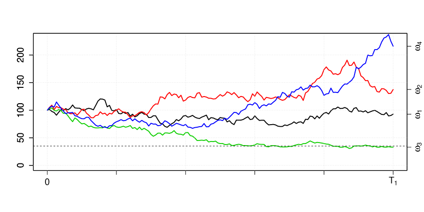
Figure 1: Simulated trajectories of the stock price. The dashed line is set at level $\exp\{{\bar{c}\}}$.

Based on the scenario $(S_{t}(\omega_{1}))_{t\geq 0}$ and different values for $\rho$, Figure 2 shows a series of simulated trajectories for the fundamental process $(U_{t})_{t\geq 0}$. As the correlation parameter tends to 1, the behavior of $(U_{t})_{t\geq 0}$ matches that of the $(\log S_{t})_{t\geq 0}$ (cf. Example 4.1 and Example 4.2).

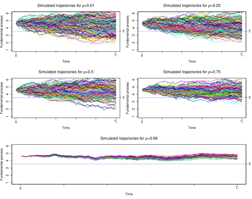
Figure 2: Simulated trajectories of the fundamental process ased on the scenario $(S_{t}(\omega_{1}))_{t\geq 0}$. The dashed line is set at level $\bar{c}$.

Finally Figure 3 shows the effect of the correlation parameter on the probability of avoiding conversion before $T_{1}$, that is, $\mathbb{P}^{*}(\tau>T_{1}|\mathcal{G}_{t})$.

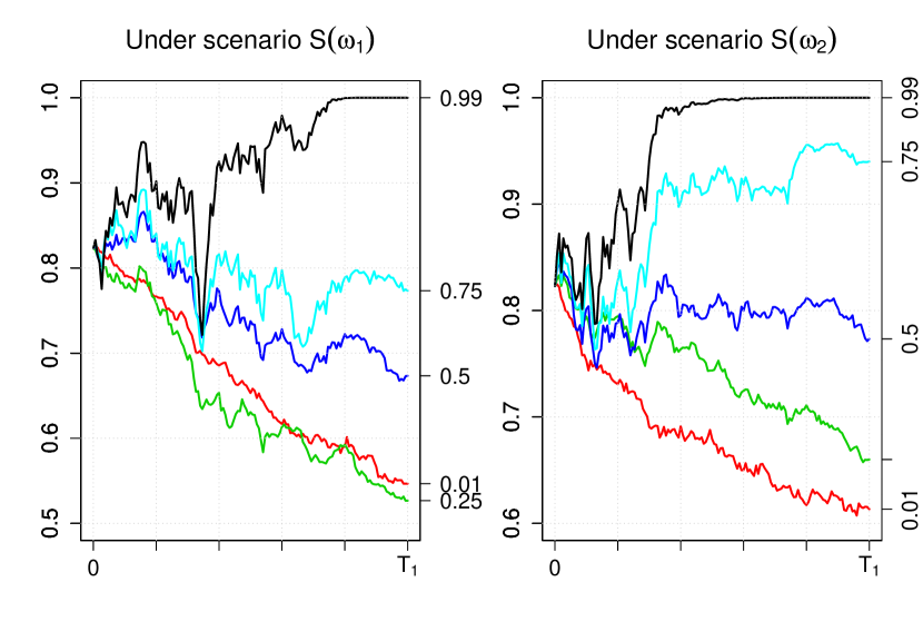
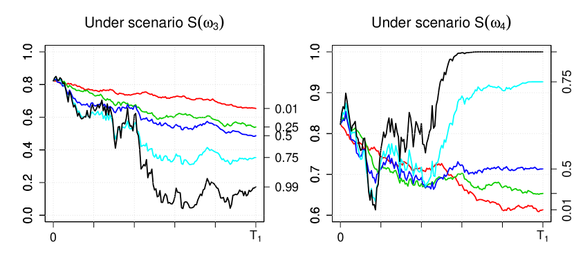
Figure 3: Simulated values for $\mathbb{P}^{*}(\tau>T_{1}|\mathcal{G}_{t})$ based on different scenarios for the stock and correlation values (marks on the seconday axis).

Appendix A Appendix

A.1 Proof of Lemma 3.2

Let us begin by showing that the process defined by $M_{t}:=\sum_{j:\;T_{j}\leq\left\lfloor t\right\rfloor}\Delta F(T_{j}),$ $t\geq 0$, follows an $\widetilde{\mathbb{F}}$-martingale. To this matter, notice that by construction $M_{t}=M_{T_{j}}=M_{s}$ whenever $T_{j}\leq s<t\leq T_{j+1}$, and thus $\mathbb{E}^{*}[M_{t}|\widetilde{F}_{s}]=M_{s}$. Now if instead we have $T_{j}\leq s<T_{j+1}\leq t<T_{j+2}$, then $M_{t}=M_{T_{j}}+\Delta F(T_{j+1})$. Again we have $M_{T_{j}}=M_{s}$. Moreover we have

$$\mathbb{E}^{*}[\Delta F(T_{j+1})|\widetilde{F}_{s}] = \mathbb{E}^{*}\left[\mathbb{P}^{*}(\tau\leq T_{j+1}|\widetilde{\mathcal{F}}_{T_{j+1}})\Big{|}\widetilde{\mathcal{F}}_{s}\right]-\mathbb{E}\left[\mathbb{P}^{*}(\tau\leq T_{j+1}^{-}|\widetilde{\mathcal{F}}_{T_{j+1}^{-}})\Big{|}\widetilde{\mathcal{F}}_{s}\right]$$

$$= \mathbb{E}^{*}\left[\mathbf{1}_{\{\tau\leq T_{j+1}\}}\Big{|}\widetilde{\mathcal{F}}_{s}\right]-\mathbb{E}^{*}\left[\mathbf{1}_{\{\tau\leq T_{j+1}^{-}\}}\Big{|}\widetilde{\mathcal{F}}_{s}\right]$$

$$= \mathbb{E}^{*}\left[\mathbf{1}_{\{\tau\leq T_{j+1}\}}-\mathbf{1}_{\{\tau<T_{j+1}\}}\Big{|}\widetilde{\mathcal{F}}_{s}\right]$$

$$= 0,$$

where the last equation follows from the fact $\mathbf{1}_{\{\tau\leq T_{j+1}\}}=\mathbf{1}_{\{\tau<T_{j+1}\}}$ since $\tau$ is defined as the hitting time of a Brownian motion.

By construction, $(A_{t})_{t\geq 0}$ is a continuous process, thus it is predictable. In order to see that it is increasing we proceed by contradiction: On the one hand, suppose that there exists $t<s$ such that $A_{t}\geq A_{s}$ a.s.; this would imply that $\mathbb{E}^{*}[A_{t}]\geq\mathbb{E}^{*}[A_{s}]$. On the other hand, since $(F_{t})_{t\geq 0}$ is an $\widetilde{\mathbb{F}}$-submartingale we have

$$\mathbb{E}^{*}[A_{s}]=\mathbb{E}^{*}[F(s)]-\mathbb{E}^{*}[M_{s}]\geq\mathbb{E}^{*}[F(t)]-\mathbb{E}^{*}[M_{s}]=\mathbb{E}^{*}[F(t)]-\mathbb{E}^{*}[M_{t}]=\mathbb{E}^{*}[A_{t}],$$

and thus the equation $\mathbb{E}^{*}[A_{s}]=\mathbb{E}^{*}[A_{t}]$ should hold. However, this would imply that $\mathbb{E}^{*}[F_{s}]=\mathbb{E}^{*}[F_{t}]$, or equivalently $\mathbb{P}^{*}(\tau\leq s)=\mathbb{P}^{*}(\tau\leq t)$, which is impossible since $\tau$ follows a strictly increasing distribution —namely the Inverse-Gaussian distribution.

A.2 The fundamental process dynamics under $\mathbb{P}^{T}$ and $\mathbb{P}^{(S)}$

The following result describes the dynamics of the processes involved in the pricing problem, both under the $T$-forward measure and share measure $\mathbb{P}^{(S)}$.

Proposition A.1.

Let $(Z_{t})_{t\geq 0}$ be a second Brownian motion, independent of $(W_{t}^{*})_{t\geq 0}$ so that we can write

$$W_{t}^{\rho}=\rho(t)W_{t}^{*}+\sqrt{1-\rho^{2}(t)}Z_{t},\qquad t\geq 0.$$

Let $\mathbb{F}^{W*}=(\mathcal{F}_{t}^{W*})_{t\geq 0}$ and let $\mathbb{F}^{Z}=(\mathcal{F}_{t}^{Z})_{t\geq 0}$ be the natural filtrations of $W*$ and $Z$ respectively. Let $(U_{t})_{t\geq 0}$ be the process defined in (10). Then (i) the process $(W_{t}^{T}:=W_{t}^{*}-\int_{0}^{t}b(t,T)\mathrm{dt})_{t\geq 0}$ (resp. $(W_{t}^{(S)}:=W_{t}^{*}-\int_{0}^{t}\sigma_{t}\mathrm{dt})_{t\geq 0}$) is an $\mathbb{F}^{W^{*}}$-Brownian motion under $\mathbb{P}^{T}$ (resp. $\mathbb{P}^{(S)}$); $(Z_{t})_{t\geq 0}$ is an $\mathbb{F}^{Z}$-Brownian motion both with respect to $\mathbb{P}^{T}$ and $\mathbb{P}^{(S)}$; and

$$(\rho(t)W_{t}^{T}+\sqrt{1-\rho^{2}(t)}Z_{t})_{t\geq 0}\qquad\left(resp.\quad(\rho(t)W_{t}^{(S)}+\sqrt{1-\rho^{2}(t)}Z_{t})_{t\geq 0}\right),$$

is a $\mathbb{G}$-Brownian motion under $\mathbb{P}^{T}$ (resp. $\mathbb{P}^{(S)}$).

(ii) The dynamics of $(U_{t})_{t\geq 0}$ under $\mathbb{P}^{T}$ are

$$\mathrm{d}U_{t} = \left(a\left\|\sigma_{t}\right\|^{2}-\frac{1}{2}\left\|\sigma_{t}\right\|^{2}+\frac{1}{2}\left\|b(t,T)\right\|^{2}+\rho(t)(\sigma_{t}-b(t,T))\cdot b(t,T)\right)\mathrm{d}t$$ (15)

$$+(\sigma_{t}-b(t,T))\cdot\left(\rho(t)\mathrm{d}W_{t}^{T}+\sqrt{1-\rho^{2}(t)}\mathrm{d}Z_{t}\right).$$

(iii) The dynamics of $(U_{t})_{t\geq 0}$ under $\mathbb{P}^{(S)}$ are

$$\mathrm{d}U_{t} = \left(a\left\|\sigma_{t}\right\|^{2}-\frac{1}{2}\left\|\sigma_{t}\right\|^{2}+\frac{1}{2}\left\|b(t,T)\right\|^{2}+\rho(t)(\sigma_{t}-b(t,T))\cdot\sigma_{t}\right)\mathrm{d}t$$ (16)

$$+(\sigma_{t}-b(t,T))\cdot\left(\rho(t)\mathrm{d}W_{t}^{(S)}+\sqrt{1-\rho^{2}(t)}\mathrm{d}Z_{t}\right).$$

Proof.

The statement about $(W_{t}^{T})_{t\geq 0}$ and $(W_{t}^{(S)})_{t\geq 0}$ follows from the Girsanov theorem. Due to the independence (under $\mathbb{P}^{*}$) between $(W_{t}^{*})_{t\geq 0}$ and $(Z_{t})_{t\geq 0}$, it is easy to see that the Lévy characterization of the Brownian motion applies to $(Z_{t})_{t\geq 0}$ and, subsequently, it also applies to $(\rho(t)W_{t}^{T}-\sqrt{1-\rho^{2}(t)}Z_{t})_{t\geq 0}$ and $(\rho(t)W_{t}^{(S)}-\sqrt{1-\rho^{2}(t)}Z_{t})_{t\geq 0}$. In light of (i), it only remains to rewrite the dynamics in (9) using the newly defined Brownian motions.∎

Notice that taking a constant interest rate implies that $\mathbb{P}^{*}$ and $\mathbb{P}^{T}$ coincide.

A.3 Conditional densities

Theorem A.2.

Let $(X_{t})_{t\geq 0}$, $(Y_{t})_{t\geq 0}$, $(Z_{t})_{t\geq 0}$ be three drifted Brownian motions under $\mathbb{P}$, with $(Z_{t})_{t\geq 0}$ independent of $(Y_{t})_{t\geq 0}$, and such that $X_{t}=Y_{t}+Z_{t}$. Let $0=t_{0}\leq t_{1}\leq...\leq t_{n}=t$ be a partition of $[0,t]$. Set the notations $X_{j}:=X_{t_{j}}$, $X^{(n)}=(X_{0},X_{1},..,X_{n})$, $x^{(n)}=(x_{0},x_{1},..,x_{n})$, and analogously for $Y$ and $Z$. Set $\tau=\inf\{t,X_{t}\leq c\}$. Then the following equation holds true

$$\mathbb{P}\left(\tau>t_{n},X^{(n)}\in\mathrm{d}x^{(n)},Y^{(n)}\in\mathrm{d}y^{(n)}\right)$$

$$= \prod\limits_{k=1}^{n}\left(1-\exp\left\{-\frac{2(x_{k}-c)(x_{k-1}-c)}{\sigma_{X}^{2}(t_{k}-t_{k-1})}\right\}\right)$$

$$\qquad\times f_{\Delta Z_{k}}(x_{k}-y_{k}-(x_{k-1}-y_{k-1)}))f_{\Delta Y_{k}}(y_{k}-y_{k-1})$$

where $\sigma^{2}_{X}:=\mathbb{E}[(X_{1}-\mathbb{E}[X_{1}])^{2}]$, and the functions $f_{\Delta Z_{k}}$ and $f_{\Delta Y_{k}}$ denote the density of $\Delta Z_{k}:=Z_{k}-Z_{k-1}$ and $\Delta Y_{k}:=Y_{k}-Y_{k-1}$, respectively.

Proof.

We have that

$$\mathbb{P}\left(\tau>t_{n},X_{n}^{(n)}\in\mathrm{d}x^{(n)},Y^{(n)}\in\mathrm{d}y^{(n)}\right)$$ (17)

$$= \mathbb{P}\left(\tau>t_{n},X_{n}\in\mathrm{d}x_{n},Y_{n}\in\mathrm{d}y_{n},X^{(n-1)}\in\mathrm{d}x^{(n-1)},Y^{(n-1)}\in\mathrm{d}y^{(n-1)}\right)$$

$$= \mathbb{P}\left(\tau>t_{n},X_{n}\in\mathrm{d}x_{n},Y_{n}\in\mathrm{d}y_{n}\Big{|}\tau>t_{n-1},X^{(n-1)}\in\mathrm{d}x^{(n-1)},Y^{(n-1)}\in\mathrm{d}y^{(n-1)}\right)$$

$$\times\mathbb{P}\left(\tau>t_{n-1},X^{(n-1)}\in\mathrm{d}x^{(n-1)},Y^{(n-1)}\in\mathrm{d}y^{(n-1)}\right)$$

$$= \mathbb{P}\left(\tau>t_{n},X_{n}\in\mathrm{d}x_{n},Y_{n}\in\mathrm{d}y_{n}\Big{|}\tau>t_{n-1},X_{n-1}\in\mathrm{d}x_{n-1},Y_{n-1}\in\mathrm{d}y_{n-1}\right)$$

$$\times\mathbb{P}\left(\tau>t_{n-1},X^{(n-1)}\in\mathrm{d}x^{(n-1)},Y^{(n-1)}\in\mathrm{d}y^{(n-1)}\right),$$

where the last equality is due to the Markovianity of $\left(\inf_{0\leq s\leq t}X_{s},X_{t},Y_{t}\right)_{t\geq 0}$. Now, by the Bayes rule

$$\mathbb{P}\left(\tau>t_{n},X_{n}\in\mathrm{d}x_{n},Y_{n}\in\mathrm{d}y_{n}\Big{|}\tau>t_{n-1},X_{n-1}\in\mathrm{d}x_{n-1},Y_{n-1}\in\mathrm{d}y_{n-1}\right)$$

$$= \frac{\mathbb{P}\left(\tau>t_{n},X_{n}\in\mathrm{d}x_{n},Y_{n}\in\mathrm{d}y_{n},X_{n-1}\in\mathrm{d}x_{n-1},Y_{n-1}\in\mathrm{d}y_{n-1}\right)}{\mathbb{P}\left(\tau>t_{n-1},X_{n-1}\in\mathrm{d}x_{n-1},Y_{n}\in\mathrm{d}y_{n}\right)}$$

$$= \mathbb{P}\left(\tau>t_{n}\Big{|}\tau>t_{n-1},X_{n}\in\mathrm{d}x_{n},Y_{n}\in\mathrm{d}y_{n},X_{n-1}\in\mathrm{d}x_{n-1},Y_{n-1}\in\mathrm{d}y_{n-1}\right)$$

$$\times\frac{\mathbb{P}\left(\tau>t_{n-1},X_{n}\in\mathrm{d}x_{n},Y_{n}\in\mathrm{d}y_{n},X_{n-1}\in\mathrm{d}x_{n-1},Y_{n-1}\in\mathrm{d}y_{n-1}\right)}{\mathbb{P}\left(\tau>t_{n-1},X_{n-1}\in\mathrm{d}x_{n-1},Y_{n}\in\mathrm{d}y_{n}\right)}$$

$$= \mathbb{P}\left(\tau>t_{n}\Big{|}\tau>t_{n-1},X_{n}\in\mathrm{d}x_{n},Y_{n}\in\mathrm{d}y_{n},X_{n-1}\in\mathrm{d}x_{n-1},Y_{n-1}\in\mathrm{d}y_{n-1}\right)$$

$$\times\mathbb{P}\left(\tau>t_{n-1},X_{n}\in\mathrm{d}x_{n},Y_{n}\in\mathrm{d}y_{n}\Big{|}\tau>t_{n-1},X_{n-1}\in\mathrm{d}x_{n-1},Y_{n-1}\in\mathrm{d}y_{n-1}\right)$$

$$= \mathbb{P}\left(\tau>t_{n}\Big{|}\tau>t_{n-1},X_{n}\in\mathrm{d}x_{n},Y_{n}\in\mathrm{d}y_{n},X_{n-1}\in\mathrm{d}x_{n-1},Y_{n-1}\in\mathrm{d}y_{n-1}\right)$$

$$\times\mathbb{P}\left(X_{n}\in\mathrm{d}x_{n},Y_{n}\in\mathrm{d}y_{n}\Big{|}X_{n-1}\in\mathrm{d}x_{n-1},Y_{n-1}\in\mathrm{d}y_{n-1}\right).$$

The last equality is true because $\left(X_{t},Y_{t}\right)_{t\geq 0}$ is Markovian. By hypothesis

$$\mathbb{P}\left(X_{n}\in\mathrm{d}x_{n},Y_{n}\in\mathrm{d}y_{n}\Big{|}X_{n-1}\in\mathrm{d}x_{n-1},Y_{n-1}\in\mathrm{d}y_{n-1}\right)$$ (18)

$$= f_{\Delta Z_{n}}(x_{n}-y_{n}-(x_{n-1}-y_{n-1}))f_{\Delta Y_{n}}(y_{n}-y_{n-1}).$$

Then, if we take $V:=X-\mathbb{E}(X)-\frac{\mathrm{Cov}(X,Z)}{\mathrm{Var}(Z)}(Z-\mathbb{E}(Z))$

$$\mathbb{P}\left(\tau>t_{n}\Big{|}\tau>t_{n-1},X_{n}\in\mathrm{d}x_{n},Y_{n}\in\mathrm{d}y_{n},X_{n-1}\in\mathrm{d}x_{n-1},Y_{n-1}\in\mathrm{d}y_{n-1}\right)$$ (19)

$$= \mathbb{P}\left(\tau>t_{n}\Big{|}\tau>t_{n-1},X_{n}\in\mathrm{d}x_{n},V_{n}\in\mathrm{d}v_{n},X_{n-1}\in\mathrm{d}x_{n-1},V_{n-1}\in\mathrm{d}v_{n-1}\right)$$

$$= \mathbb{P}\left(\tau>t_{n}\Big{|}\tau>t_{n-1},X_{n}\in\mathrm{d}x_{n},X_{n-1}\in\mathrm{d}x_{n-1}\right)$$

$$= \left(1-\exp\left\{-\frac{2(x_{n}-c)(x_{n-1}-c)}{\sigma_{X}^{2}(t_{n}-t_{n-1})}\right\}\right)\textbf{1}_{\{x_{n}>c,x_{n-1}>c\}}.$$

The last equality is a very well known result, see for instance [12, Lemma 2]. So, from (17), (18) and (19) we get the result. ∎

The densities $f_{\Delta Y_{n}}$ and $f_{\Delta Z_{n}}$ in (18) can be computed in a straightforward manner. Indeed, if we define $\mu_{Y}:=\mathbb{E}[Y_{1}]$ and $\sigma_{Y}:=\mathbb{E}[(Y_{1}-\mathbb{E}[Y_{1}])^{2}]$, then the density $f_{\Delta Y_{n}}$ corresponds to a Gaussian density with mean $\mu_{Y}(t_{n}-t_{n-1})$ and variance $\sigma_{Y}^{2}(t_{n}-t_{n-1})$, and so

$$f_{\Delta Y_{n}}(y)=\frac{1}{\sqrt{2\pi\sigma_{Y}^{2}(t_{n}-t_{n-1})}}\exp\left\{-\frac{\left(y-\mu_{Y}(t_{n}-t_{n-1})\right)^{2}}{2\sigma_{Y}^{2}(t_{n}-t_{n-1})}\right\}.$$

The expression for $f_{\Delta Z_{n}}$ is obtained analogously.

References

- [1] F. Black and J. C. Cox. Valuing corporate securities: some effects of bond indenture provisions. Journal of Finance, 31:351–367, 1976.
- [2] A.N. Borodin and P. Salminen. Handbook of Brownian motion-facts and formulae. Birkhäuser, 2012.
- [3] D. Brigo, J. Garcia, and N. Pede. Coco bonds valuation with equity- and credit-calibrated first passage structural models. Working Paper, Imperial College London, February 2013.
- [4] D. Brigo and M. Tarenghi. Credit defaulty swap calibration and equity swap valuation under counterparty risk with a tractable structural model. In Proceedings of the FEA 2004 Conference at MIT, 2004.
- [5] E. Bryis and F. de Varenne. Valuing fixed rate debt: An extension. Journal of Financial and Quantitave Analysis, 32:329–248, 1997.
- [6] D. Coculescu, H. Geman, and M. Jeanblanc. Valuation of default-sensitive claims under imperfect information. Finance Stoch., 12:195–218, 2008.
- [7] P. Collin-Dufresne, R. Goldstein, and J. Helwege. P. is credit event risk priced? modeling contagion via the updating of beliefs. Working paper, Carnegie Mellon University, 2003.
- [8] J. M. Corcuera, J. De Spiegeleer, J. Fajardo, H. Jönsson, W. Schoutens, and A. Valdivia. Close form pricing formulas for coupon cancellable cocos. Journal of Banking & Finance, 42:339–351, May 2014.
- [9] D. Duffie and D. Lando. Term structure of credit spreads with incomplete accounting information. Econometrica, 69:633–664, 2001.
- [10] X. Guo, R. A. Jarrow, and Y. Zeng. Credit risk models with incomplete information. Mathematics of Operations Research, 34(2):320–332, 2009.
- [11] P. Hieber and M. Scherer. A note on first-passage times of continuously time-changed brownian motion. Statistics and Probability Letters, 82:165–172, 2012.
- [12] M. Jeanblanc and S. Valchev. Partial information and hazard process. International Journal of Theoretical and Applied Finance, 8:807–838, 2005.
- [13] C. F. Lo, H. C. Lee, and C. H. Hui. A simple approach for pricing barrier options with time-dependent parameters. Quantitative Finance, 3:98–107, 2003.
- [14] F. A. Longstaff and E. S. Schwartz. A simple approach to valuing risky fixed and floating rate debt. Journal of Finance, 50:789–819, 1993.
- [15] R. C. Merton. On the pricing of corporate debt: The risk structure of interest rates. J. Finance, 29(2):449–470, 1974.
- [16] S. Metwally and A. Atiya. Using brownian bridge for fast simulation of jump-diffusion processes and barrier options. Journal of Derivatives, 10:43–54, 2002.
- [17] F. Rapisarda. Barrier options on underlyings with time–dependent parameters: a perturbation expansion approach. Technical Report, Product and Business Development Group, Banca IMI, May 2005.
- [18] J. Ruf and M. Scherer. Pricing corporate bonds in an arbitrary jump-diffusion model based on an improved brownian-bridge algorithm. Journal of Computational Finance, 2011.
- [19] J. Saá-Raquejo and P. Santa-Clara. Bond pricing with default risk. Working paper, UCLA, 1999.
- [20] R. Jarrow P. Protter U. Çetin and Y. Yildirim. Modelling credit risk with incomplete accounting information. Annals of applied probability, 14(3):1167–1178, 2004.
- [21] Chunsheng Zhou. The term structure of credit spreads with jump risk. Journal of Banking & Finance, 25(11):2015–2040, 2001.