Special transitions in an O($n$) loop model with an Ising-like constraint

Abstract

We investigate the O($n$) nonintersecting loop model on the square lattice under the constraint that the loops consist of ninety-degree bends only. The model is governed by the loop weight $n$, a weight $x$ for each vertex of the lattice visited once by a loop, and a weight $z$ for each vertex visited twice by a loop. We explore the $(x,z)$ phase diagram for some values of $n$. For $0<n<1$, the diagram has the same topology as the generic O($n$) phase diagram with $n<2$, with a first-order line when $z$ starts to dominate, and an O($n$)-like transition when $x$ starts to dominate. Both lines meet in an exactly solved higher critical point. For $n>1$, the O($n$)-like transition line appears to be absent. Thus, for $z=0$, the $(n,x)$ phase diagram displays a line of phase transitions for $n\leq 1$. The line ends at $n=1$ in an infinite-order transition. We determine the conformal anomaly and the critical exponents along this line. These results agree accurately with a recent proposal for the universal classification of this type of model, at least in most of the range $-1\leq n\leq 1$. We also determine the exponent describing crossover to the generic O($n$) universality class, by introducing topological defects associated with the introduction of ‘straight’ vertices violating the ninety-degree-bend rule. These results are obtained by means of transfer-matrix calculations and finite-size scaling.

I Introduction

The present work investigates the nonintersecting loop model described by the partition sum

$$Z_{{\rm loop}}=\sum_{{\rm all}\;{\mathcal{G}}}x^{N_{x}}y^{N_{y}}z^{N_{z}}n^{N_{l}},$$ (1)

where ${\mathcal{G}}$ is a graph consisting of any number of $N_{l}$ closed, nonintersecting loops. Each lattice edge may be covered by at most one loop segment, and there can be 0, 2, or 4 incoming loop segments at a vertex. In the latter case, they can be connected in two different ways without having intersections. The allowed four kinds of vertices configurations are shown in Fig. 1, together with their weights denoted $x$, $y$ and $z$. The numbers of vertices with these weights are denoted $N_{x}$, $N_{y}$, $N_{z}$ respectively.

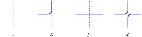
Figure 1: (Color online) The four kinds of vertices of the O($n$) loop model on the square lattice, together with their weights. Rotated versions have the same weights. The present work is mostly restricted to the subspace $(x,0,z)$ of the $(x,y,z)$ model, with a special focus on the $(x,0,0)$ subspace.

A number of such loop models in two dimensions is exactly solvable N ; Baxter ; BB ; BNW ; 3WBN ; KNB ; 3WPSN ; VF ; S ; PS ; GNB . In Ref. BNW, , five branches of critical points were found, one of which describes the densely packed loop phase, and a second branch describes its critical transition to a dilute loop gas. The latter branch describes the generic O($n$) critical behavior, and corresponds precisely with a result found earlier for the honeycomb O($n$) model N . A fifth branch found in Ref. BN, , called branch 0, is of particular interest for the present work as a special case in the $y=0$ subspace.

It is known that this generic behavior of the square-lattice O($n$) loop model can be modified by Ising-like degrees of freedom of the loop configurations BN . These degrees of freedom are exposed by placing dual Ising spins $\pm 1$ on the faces of the lattice, with the rule that nearest neighbors are of the same sign if and only if separated by a loop. Figure 2 illustrates that each $y$-type vertex corresponds with a change of sign of this Ising variable.

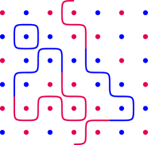
Figure 2: (Color online) Illustration of the Ising degree of freedom of O($n$) loops on the square lattice. Dual neighbor spins have opposite signs, unless separated by a loop. If $y$-type vertices are absent (left-hand side), each loop has a single Ising color. The presence of $y$-type vertices (right-hand side) leads to a change of sign of the Ising variable.

Suppression of the $y$-type vertex freezes the Ising degree of freedom of each separate loop. Thus, in the case $n=0$, where we have at most one loop, we may expect the generic O(0) behavior. For other values of $n$, the Ising degrees of freedom of adjacent loops can be different, which may influence the way they interact, and thereby modify their universal behavior. This was indeed found in earlier work FGB , using numerical investigations of the $y=0$ case. Vernier et al. VJS proposed the universal classification of this type of models as that of the generic O(2$n$) behavior. Furthermore, the phase diagram is modified for $y=0$. This will be demonstrated by the phase diagrams in the $x,z$ plane for $n=1/2$ and $n=3/2$, presented in Sec. III.1. In Sec. III we present numerical results for the conformal anomaly and the magnetic and temperature scaling dimensions. These agree well with the O(2$n$) classification, in particular for $n$ not too large. Section III also includes a determination of the topological dimension $X_{y}$ governing the crossover from the $y=0$ model to the generic O($n$) model, and a proposal for its universal classification.

A summary of the transfer-matrix technique is given in Sec. II, including some remarks on the coding of the $y=0$ connectivities, which allows us to obtain results up to finite size $L=20$. The paper concludes with a short discussion in Sec. IV.

II The transfer-matrix analysis

We consider a square O($n$) model wrapped on an cylinder with one set of edges in the length direction. The partition function of such a system with a circumference $L$ and a sufficiently large length $M$, expressed in lattice units, satisfies

$$Z(M,L)\simeq\Lambda_{0}(L)^{M}\,,$$ (2)

where $\Lambda_{0}(L)$ is the largest eigenvalue of the transfer matrix. A derivation of this formula for the present case of nonlocal interactions is given e.g., in Refs. BN82, ; WGB, . The transfer matrix indices are numbers that refer to “connectivities”, namely the way that the dangling loop segments are pairwise connected when one cuts the cylinder perpendicular to its axis. The transfer matrix technique used here is in principle the same as described in Ref. BN82, , except the coding of the “connectivities” defined there. In principle one can use the coding of the O($n$) loop connectivities described in Ref. BN, . However, the special case $y=0$ opens the possibility of a more efficient coding.

The evaluation of the largest eigenvalues of the transfer matrix is done numerically. The size of the transfer matrix increases exponentially with $L$, so that only a limited range of finite sizes can be handled. Our calculations are limited to transfer matrix sizes up to about $10^{8}\times 10^{8}$ corresponding with $L\leq 20$.

Apart from the leading eigenvalue $\Lambda_{0}(L)$, we still determine the second largest one $\Lambda_{1}(L)$. We also consider the case of a single loop segment running in the length direction of the cylinder, which actually leads to a different set of connectivities, and another sector of the transfer matrix. Its largest eigenvalue is denoted $\Lambda_{2}(L)$.

II.1 Use of the eigenspectrum

From Eq. (2) we obtain the free energy density as

$$f(L)=L^{-1}\ln\Lambda_{0}(L)\,.$$ (3)

The numerical results for $f(L)$ can be used to estimate the conformal anomaly $c$ BCN ; Affl from

$$f(L)\simeq f+\frac{\pi c}{6L^{2}}\,.$$ (4)

To avoid complications associated with alternation effects between even and odd system sizes, the present numerical work is mainly focused on even system sizes.

The gap between $\Lambda_{0}(L)$ and the subleading eigenvalues is used to determine the thermal and magnetic correlation lengths. These quantities are expressed as scaled gaps $X_{t}$ and $X_{h}$

$$X_{t}(L)=\frac{L}{2\pi}\ln\frac{\Lambda_{0}}{|\Lambda_{1}|}\,,~{}~{}~{}~{}~{}~{}X_{h}(L)=\frac{L}{2\pi}\ln\frac{\Lambda_{0}}{|\Lambda_{2}|}\,.$$ (5)

The finite-size results for the scaled gaps yield estimates of the scaling dimensions JCxi :

$$X_{t}=\lim_{L\to\infty}X_{t}(L)\,,~{}~{}~{}~{}~{}~{}X_{h}=\lim_{L\to\infty}X_{h}(L)\,.$$ (6)

These calculations are restricted to translationally invariant (zero-momentum) eigenstates of the transfer matrix.

II.2 Coulomb gas results

For the generic critical O($n$) model in two dimensions, the conformal anomaly $c$ is known BCN ; BB to be equal to

$$c=1-\frac{6(1-g)^{2}}{g},~{}~{}~{}~{}2\cos(\pi g)=-n,~{}~{}~{}~{}1\leq g\leq 2\,.$$ (7)

This range of $g$ corresponds with the critical O($n$) phase transition, but the same formula with $0\leq g\leq 1$ applies to dense phase. The scaling dimensions $X_{t}$ and $X_{h}$ of the generic O($n$) model are also known, see Ref. CG, and references therein:

$$X_{t}=\frac{4}{g}-2\,,~{}~{}~{}~{}~{}~{}~{}X_{h}=\frac{g}{8}-\frac{1}{2g}(1-g)^{2}$$ (8)

The exponent of the leading correction to scaling in the critical O($n$) model was also obtained with the Coulomb gas method CG :

$$X_{u}=2g-\frac{1}{2g}(1-g)^{2}\,,$$ (9)

II.3 Method of analysis

From Eq. (4) one may estimate the conformal anomaly from subsequent finite-size results $f(L)$ and $f(L+2)$ as

$$c(L)\equiv[f(L)-f(L+2)]\,\frac{3L^{2}(L+2)^{2}}{2\pi(L+1)}\,.$$ (10)

Taking into account corrections to scaling with exponent $y_{u}$, these estimates are expected to behave as

$$c(L)\simeq c+bL^{y_{u}}~{}~{}{\rm with}~{}~{}y_{u}=2-X_{u}\,.$$ (11)

The estimation of $c$ from the $f(L)$ is done on the basis of these two formulas and three-point fits, as described e.g., in Refs. BN82, ; FSS, . The scaling dimensions are estimated similarly from the scaled gaps defined above.

II.4 Coding for the $y=0$ case

The transfer-matrix algorithm applied in Ref. FGB, used the full set of well-nested O($n$) connectivities, i.e., the set corresponding with nonintersecting loops. However, for $y=0$, there is only a restricted set of O($n$) connectivities. If the $k$th and the $m$th edges at the end of the cylinder are occupied by dangling segments of the same loop, then $k-m$ is restricted to be odd in the absence of straight $y$-type vertices (we consider only the case of even $L$). This restriction considerably reduces the number of allowed connectivities, with more than a factor ten for the largest system size used. We wrote a new coding-decoding algorithm for this case, thus obtaining a large reduction of the size of the transfer matrix. This enabled us to handle somewhat larger systems for $y=0$ than those in past numerical studies for $y\neq 0$.   

II.5 The special case $n=1$

For $n=1$, the transfer matrix simplifies because the weights depend only on the number of loop segments, and not on the number of loops. We represent the loops by dual Ising spins $\pm 1$ such that nearest neighbors are of different signs if and only if separated by a loop. After assigning local 4-spin Ising weights $W(\hbox{\lower 2.15277pt\hbox{$+$}\hbox to0.0pt{\hss\raise 2.15277pt\hbox{$+$}}}\hbox{\lower 2.15277pt\hbox{$+$}\hbox to0.0pt{\hss\raise 2.15277pt\hbox{$+$}}})=W(\hbox{\lower 2.15277pt\hbox{$-$}\hbox to0.0pt{\hss\raise 2.15277pt\hbox{$-$}}}\hbox{\lower 2.15277pt\hbox{$-$}\hbox to0.0pt{\hss\raise 2.15277pt\hbox{$-$}}})=1$, $W(\hbox{\lower 2.15277pt\hbox{$+$}\hbox to0.0pt{\hss\raise 2.15277pt\hbox{$-$}}}\hbox{\lower 2.15277pt\hbox{$+$}\hbox to0.0pt{\hss\raise 2.15277pt\hbox{$+$}}})=x$, $W(\hbox{\lower 2.15277pt\hbox{$+$}\hbox to0.0pt{\hss\raise 2.15277pt\hbox{$-$}}}\hbox{\lower 2.15277pt\hbox{$-$}\hbox to0.0pt{\hss\raise 2.15277pt\hbox{$+$}}})=2z$, etc., one reproduces the O(1) vertex weights. Then one can easily apply a simple Ising transfer matrix, and handle system sizes up to $L=28$.

III Numerical results

The results presented in Secs. III.1 and III.2 include phase transitions that were located on the basis of the asymptotic finite-size-scaling equation

$$X_{h}(x,L)\simeq X_{h}(x,L+2)\,.$$ (12)

The vertex weight $x$ was solved numerically, with the parameters $z$ and $n$ kept constant. These solutions were denoted $x_{c}(L)$. Best estimates of $x_{c}$ were obtained after extrapolation with a procedure outlined in Ref. BN82, . Depending on the slope of a phase transition line in the $x,z$ plane, one may solve for $z$ instead while keeping $x$ constant. At $x=0$, the exact locations $z_{c}$ of the transitions follow by equating the free energy of the vacuum state to that of the completely packed state, i.e., $z_{c}=\exp[-f(n)]$ where $f(n)$ is the free energy density of the completely packed model with $z=1$. The function $f(n)$ was already found by Lieb Lieb for an equivalent 6-vertex model; for further details, see e.g. Ref. BWG, . Another exactly known critical point is the branch-0 point BN at $x=z=1/2$.

In Sec. III.1 we present the $x,z$ phase diagram for a few values of $n$. The subsections thereafter concern the estimation of the critical points and universal quantities as a function of $n$ along the critical line for $z=0$.

III.1 Phase diagrams for $n=0.5$ and $1.5$

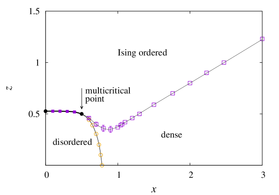
Figure 3: (Color online) Phase diagram in the $x,z$ plane for $n=1/2$. The critical O($n$) line, which separates the disordered phase from the dense O($n$) phase, is seen to merge with an Ising critical line in an exactly solved multicritical point $x=z=1/2$. For $x$ smaller than the multicritical value, the line of Ising transitions continues as a first-order line, ending at the exactly known point $x=0$, $z=0.52652729\cdots$. The other data points were numerically obtained. The curves serve only as a guide to the eye.

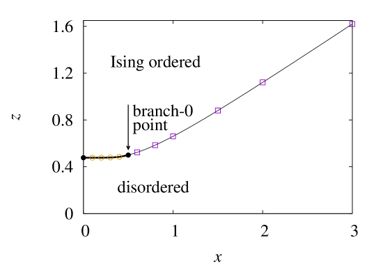
Figure 4: (Color online) Location of the Ising ordering transition in the $(x,z)$ plane of the square-lattice O(1.5) loop model. Exactly known points are shown as black circles, the other data points are numerically determined.

In both figures (Figs. 3 and  4) one observes a first-order line coming in horizontally on the vertical axis, separating the disordered phase from an Ising ordered phase. For $n=0.5$ one also observes a line of critical points where the largest loops diverge. This critical line meets the first-order line in a multicritical point called “branch 0” in Ref. BN, . A separate O($n$) critical line appears to be absent in the O(1.5) model. In both figures, the line of Ising-like transitions continues beyond the branch 0-point. The Ising-like ordered phase at larger $z$ is dominated by $z$-type vertices, and the majority of the dual Ising spins are antiferromagnetically ordered.

Although the Ising disordered phase at larger $x$ is labeled “dense” in Fig. 3, it is different from the dense phase such as described in Refs. N, ; BN, because the individual loops are already Ising ordered.

The phase diagram for the special case $n=0$ was already investigated BBN some time ago. Since there is at most one loop which is already Ising ordered, a nonzero density of that loop leads directly to a nonzero staggered magnetization of the dual spins. The question may arise if there is still an Ising-like transition for $x>0.5$ when $z$ increases. But the scaled magnetic gaps display clear intersections, indicating that there is still a phase transition line on the right-hand side of the $n=0$ diagram. This line was not observed in Ref. BBN, , which focused on the the O(0) transition line and the branch-0 point $x=z=1/2$ which was identified as a $\theta$ point describing a collapsing polymer. The numerical analysis becomes difficult in the neighborhood of $x=0.7$ for small $z$. Our interpretation, shown in Fig. 5, is that the transition line goes to $z=0$ when it approaches the O(0) line, while its critical amplitudes vanish.

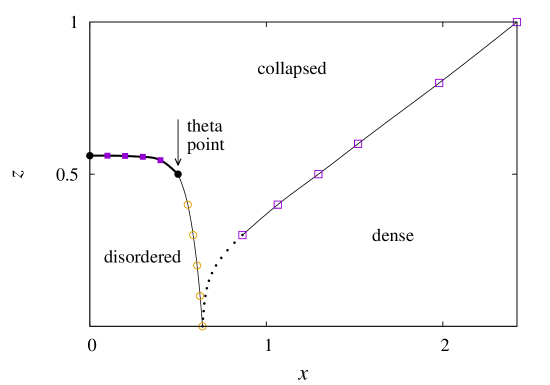
Figure 5: (Color online) Phase diagram in the $x,z$ plane for $n=0$. The O($0$) transition line on the left-hand side consists of a first-order part (thick line) and a continuous transition line going down to the $x$ axis. There is also a transition line on the right-hand side, which could be clearly located down to $z=0.3$. While the part with $z<0.3$, shown as small dots, is less accurately determined, the behavior of the magnetic gaps suggests that it continues to $z=0$.

III.2 Critical points

Critical points of the $y=z=0$ model are shown in Fig. 6 for several values of $n$ in the range $-1\leq n\leq 1$. The point $x_{c}=0.5$ at $n=-1$ is exactly known; it is equivalent with the branch-0 point of Ref. BN, because the weight $z$ is redundant at $n=-1$. The two orientations of the $z$-type vertex close a number of loops differing by precisely 1, so that summation yields 0.

Figure 6: Location of the O($n$) transition point $x_{c}$ of the $y=z=0$ model, as a function of the loop weight $n$. The error bars become visible only at the right-hand side. The line serves only as a guide to the eye.

For $n\downarrow-1$ the magnetic gap closes, implying $X_{h}\downarrow 0$, while $x_{c}$ approaches the precise value $0.5$.

For $n=1$, Eq. (12) did not yield solutions; the scaled gaps suggest marginal behavior, corresponding to an infinite-order transition. Thus we expect $X_{h}=1/8$, which is consistent with the finite-size results near the expected value of $x_{c}$. Thus we solved for $x$ in

$$X_{h}(x,L)=1/8$$ (13)

to obtain the critical point, presumably an infinite-order transition, for $n=1$. Additional estimates were obtained using the transfer matrix of the dual Ising representation and the scaling equation $X_{h}(x,L)=X_{h}(x,L+2)$, also for even system sizes.

III.3 Conformal anomaly

The conformal anomaly $c$ was numerically estimated as described in Sec. II.3. The results are shown in Fig. 7, together with the Coulomb gas prediction Eq. (7) for the O(2$n$) model. These data, which are, together with the $x_{c}$ estimates, also listed in Table 1, show that the O(2n) universal classification is quite convincing, especially for $n<0.5$, thus confirming the picture sketched in Ref. VJS, .

Figure 7: Conformal anomaly of the O($n$) model with $y=z=0$, versus the loop weight $n$. These results, shown as data points, do not agree with the predictions for the generic O($n$) model. Instead they agree well with the expected universal behavior of the O(2$n$) transition, which is shown by the curve.

Table 1: Numerical results in the range $-1\leq n\leq 1$ for the critical point $x_{c}(n)$ and the conformal anomaly $c$ of the O($n$) model with $y=z=0$. Estimated numerical uncertainties in the last decimal place are shown between parentheses. We quote zero errors in those cases where all finite-size estimates coincide within numerical precision. For comparison, we also include the exact conformal anomaly of the generic O($2n$) model.

$n$	$x_{c}(\rm num)$	$c_{\rm num}$	$c_{\rm CG}$
-1.0	0.5 (0)	-2.0000 (1)	-2.0
-0.9	0.5098053 (1)	-1.3700 (8)	-1.37061
-0.8	0.5202394 (2)	-1.11330 (3)	-1.11331
-0.7	0.5313745 (3)	-0.91570 (2)	-0.91572
-0.6	0.5432954 (5)	-0.74835 (5)	-0.748403
-0.5	0.556102 (1)	-0.59999 (2)	-0.6
-0.4	0.569913 (1)	-0.46467 (3)	-0.464687
-0.3	0.584873 (1)	-0.33898 (2)	-0.338996
-0.2	0.601158 (1)	-0.22065 (2)	-0.220651
-0.1	0.618984 (2)	-0.10805 (1)	-0.108051
0.0	0.638622 (2)	0 (0)	0
0.1	0.660420 (2)	0.10443 (1)	0.104434
0.2	0.684821 (2)	0.20602 (2)	0.206018
0.3	0.712433 (3)	0.30543 (2)	0.30541
0.4	0.74407 (1)	0.40322 (5)	0.403211
0.5	0.78090 (2)	0.5002 (1)	0.5
0.6	0.82465 (5)	0.5968 (2)	0.59639
0.7	0.8780 (2)	0.694 (2)	0.693093
0.8	0.948 (2)	0.794 (3)	0.791059
0.9	1.045 (5)	0.897 (5)	0.891858
1.0	1.20 (5)	1.02 (1)	1.0

III.4 Critical exponents

III.4.1 Magnetic dimension

The numerical results for the magnetic scaling dimension are shown as data points in Fig. 8. Since the eigenvalues $\Lambda_{0}$ and $\Lambda_{2}$ coincide for $n=-1$, one has $X_{h}=0$ exactly. The magnetic dimension of the generic O($2n$) critical point in two dimensions, given by Eq. (8), is included for comparison.

Figure 8: The data points display the results for the magnetic scaling dimension of the O($n$) model with $y=z=0$, versus the loop weight $n$. The curve shows the exactly known magnetic dimension of the generic O($2n$) model.

III.4.2 Temperature dimension

The temperature dimension was obtained from the scaled thermal gaps and the same methods of analysis as before. The results are shown as data points in Fig. 9, together with the Coulomb gas prediction Eq. (8) for the O($2n$) model.

Figure 9: Temperature scaling dimension $X_{t}$ of the O($n$) model with $y=z=0$, versus the loop weight $n$. The curve shows the exactly known temperature dimension of the generic O($2n$) model.

III.4.3 Topological dimension

As argued in Ref. BN, , the Ising degree of freedom of a loop flips whenever a $y$-type vertex occurs. Closed loops must contain an even number of these $y$-type vertices, which assume the role of topological defects. In this work we exclude these vertices by choosing $y=0$. But we can still study their effect by initializing a “defective” loop in which, e.g., dangling bonds $k$ and $k+2$ are connected. An example of such a connectivity, i.e., the way in which the dangling bonds are pairwise connected, is given in Fig. 10.

Figure 10: (Color online) An O($n$) loop connectivity with a two-colored loop. It corresponds with a topological defect if $y=0$, because such a loop cannot be closed if $y$-type vertices are absent.

This loop cannot be closed by transfer-matrix iterations if $y=0$. The presence of such a defective loop defines another transfer-matrix sector, whose leading eigenvalue we denote as $\Lambda_{3}$. Following the usual procedure, we obtain the correlation length $\xi_{y}$ describing the asymptotic behavior of the correlation function connecting two $y$-type defects along the cylinder as

$$\xi_{y}^{-1}(L)=\ln(\Lambda_{0}/\Lambda_{3})\,,$$ (14)

from which the associated scaling dimension can be obtained by extrapolation of the scaled gaps defined as

$$X_{y}(L)=\frac{L}{2\pi\xi_{y}(L)}\,.$$ (15)

The results for the scaling dimension of the $y$-type vertices are shown in Fig. 11.

Figure 11: Topological dimension $X_{y}$ of the O($n$) model with $y=z=0$, versus the loop weight $n$. The curve shows the Coulomb gas expression $1-1/2g$ as described in the text. This dimension describes the probability that two remote points of the O(2$n$) model lie on the same loop, and is equal to the conformal dimension $2\Delta_{0,1}$ of the latter model, and to the magnetic exponent of the fully-packed O($2n$) model on the honeycomb lattice FPL .

The results for $n<0.5$ are satisfactorily described by the simple formula

$$X_{y}=1-\frac{1}{2g}\,,$$ (16)

where $g$ is the Coulomb gas coupling of the critical O($2n$) model, i.e., $\cos(\pi g)=-n$ with $1\leq g\leq 2$. For $n>0.5$ the differences become larger. We believe that this is due to poor finite-size convergence associated with the proximity of a marginal scaling field at $n=1$. The numerical results for the scaling dimensions of the O($n$) model with $y=z=0$ are summarized in Table 2, together with the Coulomb gas values according to Eq. (16) for the O(2$n$) model. Again, the numerical result fits well in the O(2$n$) universality class, except in the neighborhood of $n=1$ where finite-size convergence is slow, and numerical uncertainties are easily underestimated.

Table 2: Numerical results for the scaling dimensions $X_{h}$, $X_{t}$, and $X_{y}$ of the O($n$) model with $y=z=0$. Estimated numerical uncertainties in the last decimal place are shown between parentheses. Zero errors are shown where all finite-size estimates are zero within numerical precision. For $X_{h}$, $n=1$ we quote no error because the value $X_{h}=1/8$ was assumed in the derivation of $x_{c}$. For comparison, we also include the Coulomb gas results for the generic O($2n$) model.

$n$	$X_{h,{\rm num}}$	$X_{h,{\rm CG}}$	$X_{t,{\rm num}}$	$X_{t,{\rm CG}}$	$X_{y,{\rm num}}$	$X_{y,{\rm CG}}$
-1.0	0 (0)	0	0 (0)	0	0.7500 (1)	0.75
-0.9	0.0350 (5)	0.0345037	0.153 (2)	0.154669	0.735 (5)	0.730666
-0.8	0.0486 (2)	0.0482867	0.227 (1)	0.228205	0.723 (1)	0.721474
-0.7	0.0584 (1)	0.0587088	0.2898 (1)	0.28988	0.7135 (5)	0.713765
-0.6	0.0668 (2)	0.0674038	0.3460 (3)	0.346271	0.7065 (5)	0.706716
-0.5	0.0750 (5)	0.075	0.3995 (5)	0.4	0.7000 (1)	0.7
-0.4	0.0818 (5)	0.0818165	0.4521 (5)	0.452498	0.6939 (5)	0.693438
-0.3	0.0880 (2)	0.0880403	0.5045 (2)	0.504717	0.6878 (5)	0.68691
-0.2	0.0938 (1)	0.0937908	0.5573 (2)	0.557391	0.6813 (5)	0.680326
-0.1	0.0992 (1)	0.099148	0.6112 (2)	0.611163	0.6743 (5)	0.673605
0.0	0.1042 (1)	0.104167	0.6668 (2)	0.666667	0.6675 (5)	0.666667
0.1	0.1090 (1)	0.108884	0.7252 (5)	0.724581	0.6594 (5)	0.659427
0.2	0.1134 (1)	0.113323	0.7859 (1)	0.785698	0.6504 (5)	0.651788
0.3	0.1177 (2)	0.117494	0.8509 (5)	0.851006	0.641 (1)	0.643624
0.4	0.1216 (3)	0.121394	0.921 (1)	0.921819	0.632 (1)	0.634773
0.5	0.1255 (3)	0.125	1.00 (1)	1	0.620 (2)	0.625
0.6	0.1286 (3)	0.128262	1.085 (5)	1.0884	0.608 (5)	0.613949
0.7	0.132 (2)	0.131072	1.18 (1)	1.19187	0.598 (8)	0.601016
0.8	0.132 (5)	0.133192	1.30 (2)	1.31996	0.59 (1)	0.585005
0.9	0.13 (2)	0.133934	1.45 (5)	1.49783	0.54 (1)	0.562771
1.0	0.125 (-)	0.125	1.8 (1)	2	0.47 (2)	0.5

IV Discussion

In the present loop model with $y=0$, the loops can in fact occupy one of two sublattices. Together with the $n$ possible colors of each loop, this leads in effect to a $2n$-fold degeneracy of the loops. In this work, we provide an accurate confirmation of the O($2n$) universal classification, in particular for $n<<1$. In the neighborhood of $n=1$, the finite-size results are subject to poor convergence, probably related to the irrelevant temperature exponent which is expected to become marginal for $n\uparrow 1$.

The phase diagram for $n=0.5$ shown in Sec. III.1 contains a part that is difficult to resolve, in particular the part between $x=1/2$ and $x=1$ of the critical line connecting to the multicritical point and forming the phase boundary of the Ising ordered phase. Near $x=0.7$, this transition is, because of its proximity to the O($n$)-type transition, hard to distinguish from it, and it should be emphasized that the phase diagram is not resolved here with certainty. If it is qualitatively correct, then the line $z=x^{2}$ runs through two phase transitions, implying the presence of an additional transition line for $y=0$ in Fig. 2 in Ref. FGB, .

While the present work is restricted to relatively small values of $n$, different phenomena are expected for large $n$ where the loops tend to become small and behave as hard lattice-gas particles. A line of transitions resembling the hard-square lattice-gas with nearest-neighbor exclusion was located in Ref. FGB, , separating a dilute phase from one dominated by $z$-type vertices. That result applies to the case $z=x^{2}$. But also for $z=0$ and sufficiently large $n$ one expects a transition when $x$ becomes larger, because one then approximates the lattice gas with nearest- and next-nearest-neighbor exclusion which displays a different type of transition Marq ; FBN .

The topological dimension $X_{y}$ defined in Sec. III.4.3 does not only describe the decay of the correlation function between two $y$-type defects in the infinite plane as $r^{-2X_{y}}$, but it also determines the crossover exponent $y_{y}=2-X_{y}$ describing the scaling $y\to y^{\prime}=b^{y_{y}}y$ under a rescaling by a scale factor $b$ near the $y=0$ fixed point. We do indeed observe that the renormalization exponent $y_{y}$ is relevant in the whole interval $-1\leq n\leq 1$.

- (1) B. Nienhuis, Phys. Rev. Lett. 49, 1062 (1982); J. Stat. Phys. 34, 731 (1984).
- (2) R. J. Baxter, J. Phys. A 19, 2821 (1986); J. Phys. A 20, 5241 (1987).
- (3) M. T. Batchelor and H. W. J. Blöte, Phys. Rev. Lett. 61, 138 (1988); Phys. Rev. B 39, 2391 (1989).
- (4) M. T. Batchelor, B. Nienhuis and S. O. Warnaar, Phys. Rev. Lett. 62, 2425 (1989).
- (5) S. O. Warnaar, M. T. Batchelor and B. Nienhuis, J. Phys. A 25, 3077 (1992).
- (6) Y. M. M. Knops, B. Nienhuis and H. W. J. Blöte, J. Phys. A 31, 2941 (1998).
- (7) S. O. Warnaar, P. A. Pearce, K. A. Seaton and B. Nienhuis, J. Stat. Phys. 74, 469 (1994).
- (8) V. A. Fateev, Sov. J. Nucl. Phys. 33, 761 (1981).
- (9) C. L. Schultz, Phys. Rev. Lett. 46, 629 (1981).
- (10) J. H. H. Perk and C. L. Schultz, in Proc. RIMS Symposium on Non-Linear Integrable Systems, edited by M. Jimbo and T. Miwa (World Scientific, 1983) p. 135; and in Yang-Baxter Equation in Integrable Systems, edited by M. Jimbo (World Scientific, 1990) p. 326.
- (11) W.-A. Guo, B. Nienhuis and H. W. J. Blöte, Phys. Rev. Lett. 96, 045704 (2006).
- (12) H. W. J. Blöte and B. Nienhuis, J. Phys. A 22, 1415 (1989); B. Nienhuis, Int. J. Mod. Phys. B4, 929 (1990).
- (13) Z. Fu, W.-A. Guo and H. W. J. Blöte, Phys. Rev. E 87, 052118 (2013).
- (14) E. Vernier, J. L. Jacobsen and H. Saleur, Dilute oriented loop models, arXiv:1509.07768v2 [cond-mat.stat-mech] (2015).
- (15) H. W. J. Blöte and M. P. Nightingale, Physica A (Amsterdam) 112, 405 (1982).
- (16) Y. Wang, W.-A. Guo, and H. W. J. Blöte, Phys. Rev. E 91, 032123 (2015).
- (17) H. W. J. Blöte, J. L. Cardy and M. P. Nightingale, Phys. Rev. Lett. 56, 742 (1986).
- (18) I. Affleck, Phys. Rev. Lett. 56, 746 (1986).
- (19) J. L. Cardy, J. Phys. A 17, L385 (1984).
- (20) B. Nienhuis, in Phase Transitions and Critical Phenomena, Vol. 11, eds. C. Domb and J. L. Lebowitz (Academic, London, 1987).
- (21) For a review, see e.g. M. P. Nightingale in Finite-Size Scaling and Numerical Simulation of Statistical Systems, ed. V. Privman (World Scientific, Singapore 1990).
- (22) E. H. Lieb, Phys. Rev. Lett. 18, 1046 (1967).
- (23) H. W. J. Blöte, Y. Wang, and W.-A. Guo, J. Phys. A 45, 494016 (2012).
- (24) H. W. J. Blöte, M. T. Batchelor, and B. Nienhuis, Physica A 251, 95 (1998).
- (25) H. W. J. Blöte and B. Nienhuis, Phys. Rev. Lett. 72, 1372 (1994).
- (26) H. C. Marques Fernandes, J. J. Arenzon, and Y. Levin, J. Chem. Phys. 126, 11405 (2007).
- (27) X. M. Feng, H. W. J. Blöte and B. Nienhuis, Phys. Rev. E 83, 061153 (2011).