Magneto centrifugal winds from accretion discs around black hole binaries

Abstract

We want to test if self-similar magneto-hydrodynamic (MHD) accretion-ejection models can explain the observational results for accretion disk winds in BHBs. In our models, the density at the base of the outflow, from the accretion disk, is not a free parameter, but is determined by solving the full set of dynamical MHD equations without neglecting any physical term. Different MHD solutions were generated for different values of (a) the disk aspect ratio ($\varepsilon$) and (b) the ejection efficiency ($p$). We generated two kinds of MHD solutions depending on the absence (cold solution) or presence (warm solution) of heating at the disk surface. The cold MHD solutions are found to be inadequate to account for winds due to their low ejection efficiency. The warm solutions can have sufficiently high values of $p(\gtrsim 0.1)$ which is required to explain the observed physical quantities in the wind. The heating (required at the disk surface for the warm solutions) could be due to the illumination which would be more efficient in the Soft state. We found that in the Hard state a range of ionisation parameter is thermodynamically unstable, which makes it impossible to have any wind at all, in the Hard state. Our results would suggest that a thermo-magnetic process is required to explain winds in BHBs.

1 Introduction

High resolution X-ray spectra, from Chandra and XMM-Newton, of stellar mass black holes in binaries (BHBs) show blueshifted absorption lines. These are signatures of winds from the accretion disk around the black hole (see Neilsen and Homman, 2012 and references therein)). It has been, further, shown for all BHBs that the absorption lines are more prominent in the Softer (accretion disk dominated) states (Ponti et al. 2012 and references therein).

In this paper we investigate the magneto hydrodynamic (hereafter MHD) solutions as driving mechanisms for winds from the accretion disks around BHBs - cold solutions from Ferreira (1997, hereafter F97) and warm solutions from Casse & Ferreira (2000b) and Ferreira (2004).

2 The MHD accretion disk wind solutions

We use the F97 solutions describing steady-state, axisymmetric solutions under the following two conditions: (1) A large scale magnetic field of bipolar topology is assumed to thread the accretion disk. The strength of the required vertical magnetic field component is obtained as a result of the solution (Ferreira, 1995). (2) Some anomalous turbulent resistivity is at work, allowing the plasma to diffuse through the field lines inside the disk. For a set of disk parameters, the solutions are computed from the disk midplane to the asymptotic regime, the outflowing material becoming, first, super slow-magnetosonic, then, Alfvénic and finally, fast-magnetosonic after which they recollimate. In this paper we rely on those solutions only, which cross their Alfvén surfaces before recollimating.

Because of ejection, the disk accretion rate varies with the radius even in a steady state, namely $\dot{M}_{acc}\propto r^{p}$. This radial exponent, $p$ is very important since it measures the local ejection efficiency. The larger the exponent, the more massive and slower is the outflow. Mass conservation writes

$$n^{+}m_{p}=\rho^{+}\simeq\frac{p}{\varepsilon}\frac{\dot{M}_{acc}}{4\pi\Omega_{K}r^{3}}$$ (1)

where $m_{p}$ is the proton mass and the superscript ”+” stands for the height where the flow velocity becomes sonic, $\Omega_{K}h=\varepsilon V_{K}$, where $V_{K}=\Omega_{K}r=\sqrt{GM_{BH}/r}$ ($G$: gravitational constant) is the keplerian speed and $\varepsilon=\frac{h}{r}$ is the disk aspect ratio, where $h(r)$ is the vertical scale height at the cylindrical radius $r$. Thus, the wind density is mostly dependent on $p$ and $\varepsilon$ for a given disk accretion rate $\dot{M}_{acc}$.

In the MHD models used in this paper the value of the exponent $p$ influences the extent of magnetisation in the outflow which is defined as $\sigma^{+}\simeq\frac{1}{p}\left(\frac{\Lambda}{1+\Lambda}\right)$ (F97, Casse & Ferreira 2000a) where $\Lambda$ is the ratio of the torque due to the outflow to the turbulent torque (usually referred to as the viscous torque). A magnetically dominated self-confined outflow requires $\sigma^{+}>1$. The F97 outflow models have been obtained in the limit $\Lambda\rightarrow\infty$ so that the self-confined outflows carry away all the disk angular momentum and thereby rotational energy with $\sigma^{+}\simeq 1/p\gg 1$.

For the MHD outflow (with given $\varepsilon$ and $p$) emitted from the accretion disk settled around a black hole, the important physical quantities are given at any cylindrical (r,z) by

$$n(r,z)=\frac{\dot{m}}{\sigma_{T}r_{g}}\left(\frac{r}{r_{g}}\right)^{(p-3/2)}f_{n}(y)$$ (2)

$$v_{i}(r,z)=c\left(\frac{r}{r_{g}}\right)^{-1/2}f_{v_{i}}(y)$$

$$B_{i}(r,z)=\left(\frac{\mu_{o}m_{p}c^{2}}{\sigma_{T}r_{g}}\right)^{1/2}\left(\frac{r}{r_{g}}\right)^{(-5/4+p/2)}f_{B_{i}}(y)$$ (3)

$$\tau_{dyn}(r)=\frac{2\pi r_{g}}{c}\left(\frac{r}{r_{g}}\right)^{3/2}f_{\tau}(y)$$

where $\sigma_{T}$ is the Thomson cross section, $c$ the speed of light, $r_{g}=GM_{BH}/c^{2}$ is the gravitational radius, $\mu_{o}$ the vacuum magnetic permeability, $y=z/r$ the self-similar variable and the functions $f_{X}(y)$ are provided by the solution of the full set of MHD equations. In the above expressions, $n$ is the proton number density and we consider it to be $\sim n_{H}$ (the Hydrogen number density); $v_{i}$ (or $B_{i}$) is any component of the velocity (or magnetic field) and $\tau_{dyn}=1/div\bf{V}$ (where $\bf{V}$ is the plasma velocity) is a measure of the dynamical time in the flow. The normalized disk accretion rate used in Equation 2 is defined by

$$\dot{m}=\frac{\dot{M}_{acc}(r_{g})\,c^{2}}{L_{Edd}}$$

where $L_{Edd}$ is the Eddington luminosity.

3 Observational constrains

3.1 The spectral energy distribution for the Soft and the Hard state

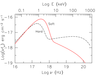
Figure 1: The SEDs corresponding to the Soft and Hard states of the outburst of a black hole of $10M_{\odot}$. The two important components of the SED, namely, the disk spectrum and the power-law have been added following the scheme described in Remillard & McClintock (2006).

We follow the prescription given in Remillard & McClintock (2006) to choose appropriate values of the relevant parameters to derive the two representative SEDs for the fiducial Soft and Hard states, for a black hole of $10M_{\odot}$ for which $r_{g}=1.5\times 10^{6}\rm{cm}$. Soft state (Figure 1 solid red curve): In the Soft state the accretion disk extends all the way to $r_{in}=3R_{s}=6r_{g}$. Thus $T(r_{in})=0.56\,{\rm keV}$. The power-law has $\Gamma=2.5$ and $A_{pl}$ is chosen in such a way that the 2-20 keV disk flux contribution $f_{d}=0.8$. Hard state (Figure 1 dotted-and-dashed black curve): With $r_{in}=6R_{s}=12r_{g}$ we generate a cooler disk with $T(r_{in})=0.33\,{\rm keV}$. The power-law is dominant in this state with $\Gamma=1.8$ and $f_{d}=0.2$. For each of the SEDs defined above, we use a high energy exponential cut-off so that there is a break in the power-law at 100 keV.

For a $10M_{\odot}$ black hole, the Eddington luminosity $L_{Edd}$ is $1.23\times 10^{39}\rm{erg\,s^{-1}}$. We define the observational accretion rate $\dot{m}_{obs}=L_{rad}/L_{Edd}$ where $L_{rad}$ is the 0.2 to 20 keV luminosity. $\dot{m}_{obs}=0.14$ using the Soft SED and is equal to $0.07$ while using the Hard SED. Thus for simplicity we assume $\dot{m}_{obs}=0.1$ for the rest of this paper.

It is important to note here, the distinction between the disk accretion rate $\dot{m}$ (Equations 2 and 2) mentioned above, and the observed accretion rate $\dot{m}_{obs}$ which is more commonly used in the literature. One can define,

$$\dot{m}=\frac{2}{\eta_{acc}}\frac{\dot{m}_{obs}}{\eta_{rad}}$$ (4)

where the factor $2$ is due to the assumption that we see only one of the two surfaces of the disk. The accretion efficiency $\eta_{acc}\simeq r_{g}/2r_{in}$ depends mostly on the black hole spin. For the sake of simplicity, we choose the Schwarzchild black hole, so that $\eta_{acc}\sim 1/12$, both in Soft and Hard state. The radiative efficiency, $\eta_{rad}=1$ if the inner accretion flow is radiatively efficient i.e. it radiates away all (or most) of the power released due to accretion. Thus $\dot{m}=2.4$.

3.2 Finding the detectable wind within the MHD outflow

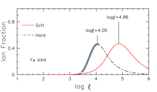
Figure 2: The ion fraction distribution of FeXXVI with respect to $\log\xi$ is shown for the two SEDs, Soft and Hard. The peak of the distribution is marked and the corresponding $\log\xi$ values are labeled. Note that for the Hard SED, a part of the distribution is highlighted by thick gray line - corresponds to the thermodynamically unstable range of $\xi$.

The MHD solutions can be used to predict the presence of outflowing material over a wide range of distances. For any given solution, this outflowing material spans large ranges in physical parameters like ionization parameter, density, column density, velocity and timescales. Only part of this outflow will be detectable through absorption lines - we refer to this part as the “detectable wind”.

We assume that at any given point within the flow, the gas is getting illuminated by light from a central point source. As such, one of the key physical parameters, in determining which region of the outflow can form a wind, is the ionization parameter $\xi=L_{ion}/(n_{H}R^{2}_{sph})$ (Tarter et al. 1969). $L_{ion}$ is the luminosity of the ionizing light in the energy range 1 - 1000 Rydberg (1 Rydberg = 13.6 eV) and $n_{H}$ is the density of the gas located at a distance of $R_{sph}$

Detected ionized gas has to be thermodynamically stable. Photoionised gas in thermal equilibrium will lie on the ‘stability’ curve of $\log T$ vs $\log(\xi/T)$ (Chakravorty et al. 2013, Higginbottom et al. 2015 and references therein). If the gas is located (in the $\xi-T$ space) on a part of the curve with negative slope then the system is considered thermodynamically unstable because any perturbation (in temperature and pressure) would lead to runaway heating or cooling. Thus we expect to detect gas which falls on the positive slope part of the curve, because it will be thermodynamically stable and will cause absorption lines in the spectrum.

Using version C08.00 of CLOUDY(hereafter C08, Ferland, 1998), we generated stability curves using both the Soft and the Hard SEDs as the ionizing continuum. For the simulation of these curves we assumed the gas to have solar metallicity, $n_{H}=10^{10}\,\,\rm{cm^{-3}}$ and $N_{H}=10^{23}\,\,\rm{cm^{-2}}$. The Soft stability curve showed no unstable region, whereas the Hard one had a distinct region of thermodynamic instability - $3.4<\log\xi<4.1$. Thus, this range of ionization parameter has to be considered undetectable, when we are using the Hard SED as the source of ionising light.

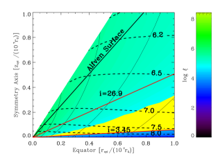
Figure 3: Top Panel: The distribution of the ‘Best Cold Set’ in the plane of the radial ($r_{cyl}$) and vertical ($z_{cyl}$) distance (in cylindrical co-ordinates, and normalised to $10^{7}r_{g}$) from the black hole. The colour gradient informs about the $\xi$ distribution of the flow. The Alfvén surface corresponding to the solution is also marked and labelled. The yellow wedge highlights the wind part of the flow - this material is optically thin with $N_{H}<10^{24}\rm{cm^{-3}}$ and has sufficiently low ionization parameter (with $\xi<10^{4.86}\rm{erg\,cm}$) to cause FeXXVI absorption lines. The angular extent of the wind is also clearly marked, where $i$ is the equatorial angle. The dashed lines show the iso-contours of $n_{H}$, while the associated labels denote the value of $\log n_{H}(\rm{cm^{-3}})$.

We choose the presence of the ion FeXXVI as a proxy for detectable winds. The probability of presence of the $X^{+i}$ ion is measured by its ion fraction $I(X^{+i})=\frac{N(X^{+i})}{f(X)\,N_{\rm{H}}}$, where $N(X^{+i})$ is the column density of the $X^{+i}$ ion and $f(X)=n(X)/n_{\rm{H}}$ is the ratio of the number density of the element $X$ to that of hydrogen. Figure 2 shows that ion fraction of FeXXVI (calculated using C08) are, of course, different based on whether the Soft or the Hard SED has been used as the source of ionization for the absorbing gas. The value of $\log\xi$, where the presence of FeXXVI is maximised, changes from 4.05 for the Hard state, by $\sim$ 0.8 dex, to 4.86 for the Soft state.

In the light of all the above mentioned observational constraints, we will impose the following physical constraints on the MHD outflows (in Sections 4 and 5) to locate the detectable wind region within them:
$\bullet$ In order to be defined as an outflow, the material needs to have positive velocity along the vertical axis ($z_{cyl}$).
$\bullet$ Over-ionized gas cannot cause any absorption and hence cannot be detected. Thus to be observable via FeXXVI absorption lines the ionization parameter of the gas needs to have an upper limit. We imposed that $\xi\leq 10^{4.86}\,\,{\rm{erg\,cm}}$ (peak of FeXXVI ion fraction) for the Soft state. For the Hard state, the constraint is $\xi\leq 10^{3.4}\,\,{\rm{erg\,cm}}$, the value below which the thermal equilibrium curve is stable.
$\bullet$ The wind cannot be Compton thick and hence we impose that the integrated column density along the line of sight satisfies $N_{H}<10^{24}{\rm{cm^{-2}}}$.

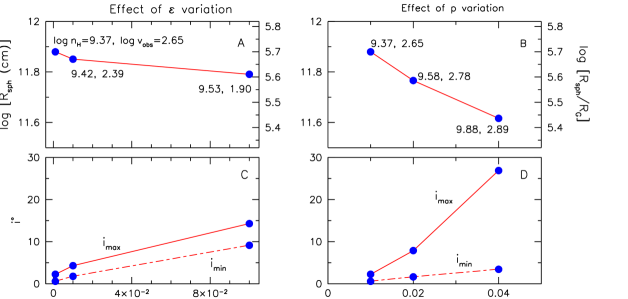
Figure 4: The physical parameters of the wind are plotted as a function of $\varepsilon$ (left panels) and $p$ (right panels), while using the Soft SED as the ionizing continua. Top Panels: For the closest wind point, we plot the logarithm of $R_{sph}|_{wind}$ in the left panel A as a function of the disk aspect ratio $\varepsilon$ and as a function of the accretion index $p$ in the right panel B. $p=0.01$ is held constant for the solutions in the left panels and $\varepsilon=0.001$ is kept constant for those in the right panels. Each blue circle in the figure represents a MHD solution. The logarithm of two other relevant quantities, $n_{H}$ and $v_{obs}$ for the closest wind point are labeled at each point - these are their maximum possible values within the wind region, for a given MHD solution. Bottom Panels: The minimum ($i_{min}$) and the maximum ($i_{max}$) equatorial angles of the line of sight, within which the wind can be observed, is plotted as a function of $\varepsilon$ (left) and of $p$ (right).

Here, we demonstrate how we choose the part of the MHD outflow which will be detectable through absorption lines of FeXXVI. For the demonstration we use the MHD solution with $\varepsilon=0.001$ and $p=0.04$ which is illuminated by the Soft SED. Hereafter we will refer to this set of parameters as the “Best Cold Set”.

We use the above mentioned physical constrains on the ‘Best Cold Set’ and get the yellow ‘wedge’ region in Figure 3. The wind is equatorial, for the ‘Best Cold Set’, not extending beyond $i=26.9^{\circ}$. The labelled dashed black lines are the iso-contours for the number density $\log n_{H}(\rm{cm^{-3}})$. We have checked that the velocities $v_{obs}$ within this region fall in the range $10^{2}-10^{3}\rm{km\,s^{-1}}$. We checked that conditions of thermal equilibrium were satisfied within the wind region of the outflow.

This same method of finding the wind, and the associated physical conditions is used for all the cold MHD solutions considered in this paper. In the subsequent sections we will vary the MHD solutions (i.e. $\varepsilon$ and $p$) and investigate the results using both the Soft and Hard SEDs.

4 The cold MHD solutions

4.1 Effect of variation of the parameters of the MHD flow

For observers, an important set of parameters are the distance ($R_{sph}|_{wind}$), density ($n_{H}|_{max}$) and velocity ($v_{obs}|_{max}$) of the point of the wind closest to the black hole. Hereafter we shall call this point as the ‘closest wind point’. Note that for any given solution, $n_{H}|_{max}$ and $v_{obs}|_{max}$ are the maximum attainable density and velocity, respectively, within the wind region. Another quantity of interest would be the predicted minimum $i_{min}$ and maximum $i_{max}$ equatorial angles (of the line of sight) within which the wind can be observed. The results are plotted in Figure 4.

$R_{sph}|_{wind}$ decreases, i.e. the winds goes closer to the black hole, as $\varepsilon$ increases (panel A of Figure 4). $n_{H}|_{max}$ increases as $\varepsilon$ increases, but $v_{obs}|_{max}$ decreases (panel A). The growth of $\Delta i=i_{max}-i_{min}$ with $\varepsilon$ (panel C) shows that the wind gets broader as the disk aspect ratio increases.

As $p$ increases, the wind moves closer to the black hole (panel B of Figure 4). The total change in $n_{H}|_{max}$ is 0.51 dex as $p$ changes from 0.01 to 0.04 (as compared to 0.16 through $\varepsilon$ variation). Both $R_{sph}|_{wind}$ and $n_{H}|_{max}$ are effected more by the variation in $p$ than by the variation in $\varepsilon$ The growth of $\Delta i$ (panel D) is also higher as a function of increase in $p$, implying a higher probability of detecting a wind when the flow corresponds to higher $p$ values. Thus, $p$ is the relatively more dominant (compared to $\varepsilon$) disk parameter to favour detectable winds.

4.2 Cold solutions for the Hard state

For the entire range of $\varepsilon$ (0.001 - 0.1) and $p$ (0.1 - 0.4) we analysed the MHD solutions illuminated by the Hard SED, as well. Note that for the Hard SED, we have to modify the upper limit of $\xi$ according to the atomic physics and thermodynamic instability considerations (Section 3.2). With the appropriate condition, $\log\xi\leq 3.4$, we could not find any wind regions within the Compton thin part of the outflow, for any of the MHD solutions. This is a very significant result, because this provides strong support to the observations that BHBs do not have winds in the Hard state.

4.3 Cold solutions cannot explain observed winds

For most of the observed BHB winds the reported density $\geq 10^{11}\,\rm{cm^{-3}}$ the distance $\leq 10^{10}\,\rm{cm}$ (Schulz & Brandt, 2002; Ueda et al. 2004; Kubota et al. 2007; Miller 2008; Kallman, 2009). Compared to these observations, for even the ‘Best Cold Solution’, $R_{sph}|_{wind}$ is too high and $n_{H}|_{max}$ is too low. The same analysis indicates that a MHD solutions with higher $\varepsilon$, say 0.01, and a high $p\geq 0.04$ would be the better suited to produce detectable winds, comparable to observations. However it is not possible to reach larger values of $p$ for the cold solutions with isothermal magnetic surfaces.

Within the steady-state approach of near Keplerian accretion discs, the magnetic field distribution is related to $p$ via Equation 3. Note that these Ferreira et al. MHD solutions, assume that the magnetic flux threading the disk is a result of the balance between outward turbulent diffusion and inward advection of the magnetic field. One might argue that cold solutions with larger values of $p$ may be generated if the condition of the balance is relaxed (i.e. if magnetic flux is either continuously advected inward, e.g. in magnetized advection-dominated discs, or if magnetic flux continuously diffuses outward). However, to relax the balance, one needs to relax either the steady-state assumption or relax the Keplerian assumption. It is not clear that whether self-similarity conditions will hold, if these aforementioned assumptions are relaxed. Note that in the context of AGN, Fukumura et al. (2010a, 2010b, 2014, 2015) have been able to reproduce the various components of the absorbing gas using MHD outflows which would correspond to $p\simeq 0.5$, a value much higher than in our best cold solution. Looking at the MHD solutions used by them (Contopoulos & Lovelace, 1984), one cannot simply say that it is the outcome of non-steady balance. Further, they have not relaxed the steady-state assumption or the Keplerian assumption - their solutions remain self-similar out to $r_{out}=10^{6}r_{in}$.

One way to get denser outflows with larger $p$, while keeping the assumption which ensure self-similar solutions, is to consider some entropy generation at the disc surface - this automatically leads to a magnetic field distribution that is different from the usual Blandford & Payne (1982) one. The disk surface heating may be the result of illumination from the inner accretion disk or of enhanced turbulent dissipation at the base of the corona. For such flows, larger values of $p$ up to $\sim 0.45$ have been reported (Casse and Ferreira, 2000b; Ferreira, 2004).

5 Warm MHD solutions

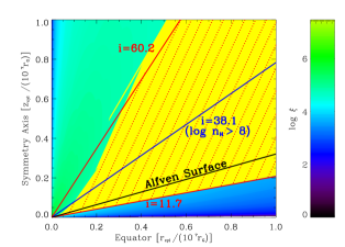
Figure 5: The ionization parameter distribution for a Warm MHD solution with $\varepsilon=0.01$ and $p=0.10$. The yellow region within the outflow is obtained in the same way as in Figure 3. The shaded region (with dotted red lines) is the wind region within such a warm outflow - to obtain this region we used the additional constraint that the cooling timescale of the gas has to be lower than the dynamical time scale. Further, the solid blue line with $i=38.1^{\circ}$ is drawn to depict that high density material ($\log n_{H}\geq 8.0$) in the flow is confined to low equatorial angles.

For the current analysis, we obtain dense warm solutions (with $p\geq 0.04$) through the use of an ad-hoc heating function. We use the same shape for the heating function, while playing only with its normalization - the larger the heat input, the larger the value of $p$. For $\varepsilon=0.01$ we could achieve a maximum value of $p=0.11$.

Figure 5 shows the wind for a Warm MHD solution with $p=0.10$. The wind (yellow region) spans a much wider range and extends far beyond the Alfvén surface which was not the case for the cold MHD solutions. Hence we introduced an additional constraint - the cooling timescale (calculated using C08) needs to be shorter than the dynamical timescale - which was satisfied within the yellow region if $i\leq 60^{\circ}$. Thus the red-dotted shaded region is the resultant detectable wind. However, note that the densest parts of the wind is still confined to low equatorial angles - e.g. gas with $n_{H}\geq 10^{8}\,\rm{cm^{-3}}$ will lie below $i=38.1^{\circ}$.

We investigated warm MHD solutions with a range of $p$ values (Figure 6). $R_{sph}|_{wind}$ goes closer by a factor of 3.79 and stands at $7.05\times 10^{4}\,r_{g}$, when $p$ increases from 0.04 to 0.11. The highest density that we could achieve is $\log n_{H}=11.1$ and the highest velocity is $\log v_{obs}=3.43$. Hereafter we shall refer to the $\varepsilon=0.01$ and $p=0.10$ warm MHD solution as the “Best Warm Solution”.

Clearly, warm solutions do a much better job than cold ones, as expected. However, some observational results require the winds to have higher density and lower distance than those produced by the “Best Warm Solution”.

We showed in Section 4.2 that with the appropriate restrictions (due to thermodynamic instability) on the $\xi$ value, no wind could be found within the cold MHD outflows, in the Hard state. Since the warm solutions result in much broader (than that in cold solutions) wind region, we tested if the best warm solution can have a wind with a Hard SED. We use the constraint that to be a detectable wind in the Hard state, the gas has to have $\log\xi<3.4$. Like the case of “best cold solution”, here also we do not find any wind region.

6 Discussions and Conclusions

6.1 Choice of upper limit of $\xi$

We used the limit $\log\xi\leq 4.86$ to define the detectable wind. Note that for the Soft SED, $\log\xi=4.86$ corresponds to the peak of the ion fraction of FeXXVI (Figure 2). The ion can have significant presence at higher $\xi$.

For the best warm solution we calculated the physical parameters for the closest wind point for $\log\xi\leq 6.0$. We find that $R_{sph}|_{wind}$ decreases by a factor of 93.4 bringing this point to $9.1\times 10^{2}r_{g}$. The density at this point is $\log n_{H}=13.71$ and the velocity is $\log v_{obs}=4.28$. Thus we see that the parameters of closest point is sensitively dependant on the choice of the upper limit of $\xi$.

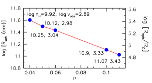
Figure 6: Distance (density and velocity) of the closest wind point is (are) plotted (labelled) as a function of $p$ for all the warm MHD solutions that we investigated. $\varepsilon=0.01$ is constant.

6.2 The need for denser warm solution

As mentioned before, the Fukumura et.al. papers use MHD solutions with $p\simeq 0.5$ to model AGN outflows. We have not been able to reproduce such high values of $p$ and are limited to $p=0.11$, at present. Our calculations show that as $p$ increased from 0.04 to 0.11 for the warm MHD solution, $R_{sph}|_{wind}$ for the closest wind point decreased by a factor of 3.79. Thus a further increase to $p\simeq 0.5$ may take the closest wind point nearer to the black hole (hypothetically) by a further factor of $\sim 10$, to $\sim 5\times 10^{3}r_{g}$ (assuming an almost linear change in density as $p$ increases). We shall report the exact calculations in our future publications.

7 Conclusions

In this paper we investigated if magneto centrifugal outflows (Ferreira, 1997; Casse & Ferreira 2000b) can reproduce the observed winds. The investigations are done as a function of the two key accretion disk parameters - the disk aspect ratio $\varepsilon$ and the radial exponent $p$ of the accretion rate ($\dot{M}_{acc}\propto r^{p}$). The results are summarised below:
$\bullet$ We need high values of $p(>0.04)$ to reproduce winds that can match observations. However $p$ cannot be increased to desirable values in the framework of the cold MHD solutions. We definitely need warm MHD solutions to explain the observational results.
$\bullet$ In the Soft state, our densest warm MHD solution predicts a wind at $7.05\times 10^{4}r_{g}$ with a density of $\log n_{H}=11.1$. The densest part of the wind ($\log n_{H}>8$) still remains equatorial - within $i\sim 30^{\circ}$ of the accretion disk. The values of the physical parameters are consistent with some of the observed winds in BHBs.
$\bullet$ The outflow illuminated by a Hard SED will not produce detectable wind because the wind region falls within the thermodynamically unstable range of $\log\xi$ and hence unlikely to be detected. Further in the absence of favourable illumination, it is likely that the Hard state will have an associated cold outflow, which is incapable of producing the usually observed winds. When these two aspects are considered together, we realise that it is impossible to ever produce a wind in the canonical Hard state.