Breather-to-soliton and rogue wave-to-soliton transitions in a resonant erbium-doped fiber system with higher-order effects

Abstract

Under investigation in this paper is the higher-order nonlinear Schrödinger and Maxwell-Bloch (HNLS-MB) system which describes the wave propagation in an erbium-doped nonlinear fiber with higher-order effects including the fourth-order dispersion and quintic non-Kerr nonlinearity. The breather and rogue wave (RW) solutions are shown that they can be converted into various soliton solutions including the multipeak soliton, periodic wave, antidark soliton, M-shaped soliton, and W-shaped soliton. In addition, under different values of higher-order effect, the locus of the eigenvalues on the complex plane which converts breathers or RWs into solitons is calculated.

1 Introduction

Optical solitons have attracted considerable interest of scientists around the world during the past decades OP . In optical fibers, there are two different types of solitons. One is described by the nonlinear Schrödinger (NLS) equation NLSS ; NLSS_1 , the mechanism of which is based on the balance between the second-order dispersion and Kerr nonlinearity. This type of soliton is called the NLS soliton. The other type of lossless pulse propagation is the self-induced transparency (SIT) soliton in the two-level resonance medium, the dynamic response of which is governed by the Maxwell-Bloch (MB) system MB . When erbium is doped with the core of the optical fibers, the NLS soliton can exist with the SIT soliton. The propagation of such pluse can be modeled by the NLS-MB system NLSMB ; NLSMB_1 ; NLSMB_2 ; NLSMB_3 ; NLSMB_4 . However, in an optical-fiber transmission system, one always needs to increase the intensity of the incident light field to produce ultrashort optical pulses High ; High_1 ; High_2 ; High_3 ; High_4 . Thus, such higher-order effects as the higher-order dispersion, higher-order nonlinearity, self-steepening, and self-frequency shift, should be included High ; High_1 ; High_2 ; High_3 ; High_4 .

In this paper, we will work on the higher-order NLS-MB system as follows GNLS_MB ; GNLS_MB1 ; GNLS_MB2 ; GNLS_MB3 ; GNLS_MB4 ,

$$E_{z}= i\,(E_{tt}+2\,|E|^{2}\,E)+i\,\tau\,(E_{tttt}+8\,|E|^{2}\,E_{tt}$$ (1.1)

$$+2\,E^{2}\,E_{tt}^{\ast}+6\,E^{\ast}\,E_{t}^{2}+4\,|E_{t}|^{2}\,E$$

$$+6\,|E|^{4}\,E)+2\,p\,,$$

$$p_{t}= 2i\,\omega p+2\,E\eta,$$

$$\eta_{t}= -(Ep^{*}+E^{*}p)\,.$$

where the subscripts $z$, $t$ are partial derivatives with respect to the distance and time, the asterisk symbol stands for the complex conjugate. $E$ denotes the normalized slowly varying amplitude of the complex field envelope, $p=v_{1}v^{*}_{2}$ represents as the polarization, and $\eta=|v_{1}|^{2}-|v_{2}|^{2}$ means the population inversion with $v_{1}$ and $v_{2}$ being the wave functions of the two energy levels of the resonant atoms, $\omega$ is the frequency, $\tau$ is a small dimensionless real parameter.

Various solutions of System (1.1) have been discussed. For example, based on the Lax pair and Darboux transformation (DT), the multi-soliton solutions of System (1.1) have been presented in Ref. GNLS_MB . The breather, rogue wave (RW) and hybrid solutions of System (1.1) have been obtained by means of the generalized DT in Refs. GNLS_MB1 ; GNLS_MB2 ; GNLS_MB3 ; GNLS_MB4 . Solitons, breathers, and RWs are different types of nonlinear localized waves and are central objects in diverse nonlinear physical systems ND ; ND1 ; ND2 ; ND3 ; ND4 ; ND5 ; ND6 ; ND7 ; ND8 ; ND9 ; ND10 . The hybrid solutions, which are expressed in forms of the mixed rational-exponential functions, describe the nonlinear superposition of the RW and breather hi . Recently, Liu et al. have shown that the breathers can be converted into different types of nonlinear waves in the coupled NLS-MB system, including the multipeak soliton, periodic wave, antidark soliton, and W-shaped soliton Liu . These conversions occur under a special condition in which the soliton and a periodic wave in the breather have the same velocity Liu . In addition, the similar transitions have also been reported in some higher-order nonlinear equation of evolutions. Akhmediev et al. have found that the breather solutions of the Hirota A-Hirota equation and fifth-order NLS A-FNLS equation can be converted into soliton solutions on the constant background, which does not exist in the standard NLS equation. Liu et al. have revealed that the transition between the soliton and RW occurs as a result of the attenuation of MI growth rate to vanishing in the zerofrequency perturbation region Hirota ; Hirota_1 .

It is natural to ask: Can the transition between the breather (or RW) and soliton occur in the higher-order coupled system, e.g., System (1.1)? In this paper, we show that System (1.1) does have such transition when the eigenvalues are located at the special locus on the complex plane. Further, we demonstrate that the breather can be converted into the multipeak soliton, periodic wave, antidark soliton, and M-shaped soliton while the RW can be transformed into the W-shaped soliton.

The outline of this paper will be as follows: The breather-to-soliton conversion and several types of transformed nonlinear waves will be studied in Section 2. The RW-to-soliton conversion will be discussed in Section 3. Finally, our conclusions will be addressed in Section 4.

2 Breather-to-soliton conversions

In this section, we present different types of nonlinear wave solutions on constant background for System (1.1). We omit the discussions of the components $p$ and $\eta$ because the types of them have the similar characteristics as $E$. Based on the lax pair and DT GNLS_MB ; GNLS_MB1 ; GNLS_MB2 ; GNLS_MB3 ; GNLS_MB4 of System (1.1), the first-order symmetric breather solution reads as

$$E_{B}^{[1]}= d\,(1+8\,n\,\frac{G_{B}^{[1]}+i\,H_{B}^{[1]}}{D_{B}^{[1]}})\,e^{i\,\rho}\,,$$ (2.1)

$$p_{B}^{[1]}= \frac{1}{2}\,((E_{B}^{[1]})_{z}-i\,((E_{B}^{[1]})_{tt}+2\,|E_{B}^{[1]}|^{2}\,E_{B}^{[1]})-i\,\tau((E_{B}^{[1]})_{tttt}$$

$$+8\,|E_{B}^{[1]}|^{2}\,(E_{B}^{[1]})_{tt}+2\,(E_{B}^{[1]})^{2}(E_{B}^{[1]})_{tt}^{\ast}+6\,(E_{B}^{[1]})^{\ast}$$

$$(E_{B}^{[1]})_{t}^{2}+4\,|(E_{B}^{[1]})_{t}|^{2}\,E_{B}^{[1]}+6\,|E_{B}^{[1]}|^{4}\,E_{B}^{[1]}))\,,$$

$$\eta_{B}^{[1]}= \frac{-2\,i\,\omega\,(p_{B}^{[1]})^{[1]}+(p_{B}^{[1]})_{t}^{[1]}}{2\,E_{B}^{[1]}}\,.$$

where

$$G_{B}^{[1]}=2\,k_{1}\,k_{2}\,n\,\cos(t\,h_{R}+z\,\varpi_{B})+2\,n\,\cosh(t\,h_{I}+z\,\varpi_{A})$$

$$~{}~{}~{}~{}~{}~{}~{}~{}-k_{1}\,k_{2}\,h_{R}\,\sin(t\,h_{R}+z\,\varpi_{B})+h_{I}\,\sinh(t\,h_{I}+z\,\varpi_{A})\,,$$

$$H_{B}^{[1]}=k_{1}\,k_{2}\,(b+2\,m)\,\cos(t\,h_{R}+z\,\varpi_{B})+(b+2\,m)\,\cosh(t\,h_{I}$$

$$~{}~{}~{}~{}~{}~{}~{}~{}+z\,\varpi_{A})+k_{1}\,k_{2}\,h_{I}\,\sin(t\,h_{R}+z\,\varpi_{B})+h_{R}\,\sinh(t\,h_{I}$$

$$~{}~{}~{}~{}~{}~{}~{}~{}+z\,\varpi_{A})\,,$$

$$D_{B}^{[1]}=k_{1}\,k_{2}\,(|h|^{2}-\chi)\,\cos(t\,h_{R}+z\,\varpi_{B})-(|h|^{2}+\chi)\,\cosh(t\,h_{I}$$

$$~{}~{}~{}~{}~{}~{}~{}~{}+z\,\varpi_{A})-k_{1}\,k_{2}\,\Gamma_{A}\,\sin(t\,h_{R}+z\,\varpi_{B})-\Gamma_{B}\,\sinh(t\,h_{I}$$

$$~{}~{}~{}~{}~{}~{}~{}~{}+z\,\varpi_{A})\,,$$

with

$$\rho=\,a\,z+b\,t\,,~{}~{}\lambda=m+i\,n\,,$$

$$a=(b^{4}-12\,b^{2}\,d^{2}+6\,d^{4})\,\tau-(b^{2}-2\,d^{2})+\frac{4}{2\,\omega-b}\,,$$

$$\chi=4\,m^{2}+4\,n^{2}+4\,m\,b+b^{2}+4\,d^{2}\,\,,$$

$$\Gamma_{A}=2\,b\,h_{I}+4\,m\,h_{I}-4\,n\,h_{R}\,,$$

$$\Gamma_{B}=2\,b\,h_{R}+4\,m\,h_{R}+4\,n\,h_{I}\,,$$

$$\varpi_{A}=2(\kappa_{R}\,h_{I}+\kappa_{I}\,h_{R})\,,$$

$$\varpi_{B}=2(\kappa_{R}\,h_{R}-\kappa_{I}\,h_{I})\,,$$

$$\kappa=\frac{1}{2}(-b+2\,\lambda+(b^{3}-6\,b\,d^{2}+(4\,d^{2}-2\,b^{2})\,\lambda+4\,b\,\lambda^{2}$$

$$~{}~{}~{}~{}~{}-8\,\lambda^{3})\,\tau)-\frac{1}{(b-2\,\omega)(\lambda+\omega)}=\kappa_{R}+i\,\kappa_{I}\,,$$

$$h=2\,\sqrt{d^{2}+(\lambda+\frac{b}{2})^{2}}=h_{R}+i\,h_{I}\,.$$

Solution (2.1) includes the hyperbolic functions $\sinh$
$(t\,h_{I}+z\,\varpi_{A})$ ( or $\cosh(t\,h_{I}+z\,\varpi_{A})$) and the trigonometric functions $\sin(t\,h_{R}+z\,\varpi_{B})$ (or $\cos(t\,h_{R}+z\,\varpi_{B})$), where $\kappa_{R}+\frac{\kappa_{I}h_{R}}{h_{I}}$ and $\kappa_{R}-\frac{\kappa_{I}h_{I}}{h_{R}}$ are the corresponding velocities. In this case, the hyperbolic functions and trigonometric functions, respectively, characterize the localization and the periodicity of the transverse distribution $t$ of those waves. The nonlinear structure described by Solution (2.1) can be seen as a nonlinear combination of a soliton with the velocity $\kappa_{R}+\frac{\kappa_{I}h_{R}}{h_{I}}$ and a periodic wave with the velocity $\kappa_{R}-\frac{\kappa_{I}h_{I}}{h_{R}}$. Next, we will display various nonlinear wave structures depending on the values of velocity difference, namely, $\frac{\kappa_{I}(h_{R}^{2}+h_{I}^{2})}{h_{R}h_{I}}$.

If the velocity difference is not equal to zero, i.e., $\kappa_{I}(\frac{h_{R}^{2}+h_{I}^{2}}{h_{R}h_{I}})\neq 0$ (or $k_{I}\neq 0$), Solution (2.1) characterizes the localized waves with breathing behavior on a plane-wave background (i.e., the breathers and RWs). Further, if $m=-\frac{b}{2}$, we have the Akhmediev breathers with $|n|<|d|$, the Kuanetsov-Ma solitons with $|n|>|d|$, and the Peregrine soliton with $|n|=|d|$. Such solutions have been derived in Refs. GNLS_MB1 ; GNLS_MB2 ; GNLS_MB3 ; GNLS_MB4 (also see Fig. 1).

Instead, if $\kappa_{I}=0$, the wave described by Solution (2.1) is composed of a soliton and a periodic wave, where each has the same velocity $\kappa_{R}$. It should be noted that the case $\kappa_{I}=0$ is equivalent to

$$\frac{\varpi_{A}}{h_{I}}=\frac{\varpi_{B}}{h_{R}}\,,$$ (2.2)

i.e.,

$$\tau=\frac{\Theta_{1}}{\Theta_{2}}\,,$$ (2.3)

where

$$\Theta_{1}=(b-2\omega)\left((m+\omega)^{2}+n^{2}\right)+1\,,$$

$$\Theta_{2}=(b-2\omega)\left((m+\omega)^{2}+n^{2}\right)(b^{2}-4bm-2(d^{2}-$$

$$~{}~{}~{}~{}~{}~{}~{}~{}6m^{2}+2n^{2}))\,.$$

Eq. (2.2) [i.e., Eq. (2.3)] implies the extrema of trigo-nometric and hyperbolic functions in Solution (2.1) is located along the same straight lines in the $(z,t)$-plane, which leads to the transformation of the breather into a continuous soliton. Choosing different values of $\tau$ in Eq. (2.3), we display the locus of the real and imaginary parts of the eigenvalues on the complex plane in Fig. 2. It is found that the higher-order effect $\tau$ can alter the shape of the locus. By decreasing the value of $\tau$, we find that the quantity of branches of the locus is reduced from three to two.

When the five parameters $m$, $n$, $\omega$, $\tau$, $b$ and $d$ satisfy Eq. (2.3), Expressions (2.1) describe the soliton on constant background, as depicted in Fig. 3. This type of multi-peak structure is because of the mixture of a soliton and a periodic wave. The similar multi-peak structures have been observed analytically in the NLS-MB equations Liu and numerically in the AC-driven damped NLS system mp ; mp_1 . Further, to exhibit the effect of the real part ($m$) of the eigenvalue on the peak number, we plot Fig. 4 where the soliton has significantly less peaks than the one in Fig. 3. On the other hand, due to the different choices of the value of the eigenvalue, Fig. 5 shows the soliton with two main peaks, which is referred to as the M-shaped soliton in this paper. Note that the multi-peak solitons in Figs. 3$\sim$5 are the localized structures along the $t$ axis. However, changing the values of the real and imaginary parts of eigenvalue, we display another type of solution that shows a type of nonlocal structure, i.e., the periodic wave (see Fig. 6). Therefore, it is concluded that the structure (peak number and localization) of the multi-peak soliton can be controlled by the real and imaginary parts of eigenvalue, namely, $m$ and $n$.

In order to better understand this multi-peak structure of System (1.1), we will extract separately the soliton and periodic wave from the mixed solution (2.1). Specifically, the soliton exists in isolation when $h_{R}$ vanishes, while the periodic wave independently exists when $h_{I}$ vanishes. Correspondingly, the analytic expressions read, for the antidark soliton,

$$E_{S}^{[1]}= d\,(1+8\,n\,\frac{G_{S}^{[1]}+i\,H_{S}^{[1]}}{D_{S}^{[1]}})\,e^{i\,\rho}$$ (2.4)

with

$$G_{S}^{[1]}=2\,n\,\cos(2\,z\,\kappa_{I}\,h_{I})+2\,n\,\cosh(t\,h_{I}+2\,z\,\kappa_{R}\,h_{I})$$

$$~{}~{}~{}~{}~{}~{}~{}~{}+h_{I}\,\sinh(t\,h_{I}+2\,z\,\kappa_{R}\,h_{I})\,,$$

$$H_{S}^{[1]}=\,(b+2\,m)\,\cos(2\,z\,\kappa_{I}\,h_{I})+(b+2\,m)\,\cosh(t\,h_{I}$$

$$~{}~{}~{}~{}~{}~{}~{}~{}+2\,z\,\kappa_{R}\,h_{I})-\,h_{I}\,\sin(2\,z\,\kappa_{I}\,h_{I})\,,$$

$$D_{S}^{[1]}=\,(h_{I}^{2}-\chi)\,\cos(2\,z\,\kappa_{I}\,h_{I})-(h_{I}^{2}+\chi)\,\cosh(t\,h_{I}$$

$$~{}~{}~{}~{}~{}~{}~{}~{}+2\,z\,\kappa_{R}\,h_{I})+\,(2\,b\,h_{I}+4\,m\,h_{I})\,\sin(2\,z\,\kappa_{I}\,h_{I})$$

$$~{}~{}~{}~{}~{}~{}~{}~{}-4\,n\,h_{I}\,\sinh(t\,h_{I}+2\,z\,\kappa_{R}\,h_{I})\,,$$

and for the periodic wave,

$$E_{P}^{[1]}= d\,(1+8\,n\,\frac{G_{P}^{[1]}+i\,H_{P}^{[1]}}{D_{P}^{[1]}})\,e^{i\,\rho}$$ (2.5)

with

$$G_{P}^{[1]}=-2\,n\,\cos(t\,h_{R}+2\,z\,\kappa_{R}\,h_{R})+2\,n\,\cosh(2\,z\,\kappa_{I}\,h_{R})$$

$$~{}~{}~{}~{}~{}~{}~{}~{}~{}+\,h_{R}\,\sin(t\,h_{R}+2\,z\,\kappa_{R}\,h_{R})\,,$$

$$H_{P}^{[1]}=-\,(b+2\,m)\,\cos(t\,h_{R}+2\,z\,\kappa_{R}\,h_{R})+(b+2\,m)$$

$$~{}~{}~{}~{}~{}~{}~{}~{}~{}\cosh(2\,z\,\kappa_{I}\,h_{R})+h_{R}\,\sinh(2\,z\,\kappa_{I}\,h_{R})\,,$$

$$D_{P}^{[1]}=-\,(h_{R}^{2}-\chi)\,\cos(t\,h_{R}+2\,z\,\kappa_{R}\,h_{R})-(h_{R}^{2}+\chi)$$

$$~{}~{}~{}~{}~{}~{}~{}~{}~{}\cosh(2\,z\,\kappa_{I}\,h_{R})-4\,n\,h_{R}\,\sin(t\,h_{R}+2\,z\,\kappa_{R}\,h_{R})$$

$$~{}~{}~{}~{}~{}~{}~{}~{}-(2\,b\,h_{R}+4\,m\,h_{R})\,\sinh(2\,z\,\kappa_{I}\,h_{R})\,.$$

Fig. 7 describes a soliton on the constant background, which propagates along $t$ direction. This kind of soliton is called the antidark soliton firstly reported in the scalar NLS system with the third-order dispersion ANTI ; ANTI_1 . Futher, as $d$ is approaching to zero, this soliton will turn into a standard bright soliton. Fig. 8 is plotted for the periodic waves propagating in $t$ direction with the period $P=\frac{\pi}{h_{R}}$.

3 RW-to-soliton conversion

In this section, we investigate the transition of first-order localized wave $|E_{1}(t,z)|^{2}$ from the RW to the W-shaped traveling wave. Taking $\lambda\rightarrow-\frac{b}{2}+i\,d$ in Solution (2.1), we obtain the first-order RW which is asymmetric with respect to $z$-axis in Fig. 9. Further, to convert the asymmetric RW into a soliton, the parameters $\omega$, $\tau$ and $b$ have to satisfy Eq. (2.3). Unlike the cases in Section 2, such transition is only controlled by three free parameters due to the fixed values of the real ($m=-\frac{b}{2}$) and imaginary ($n=d$) parts of the eigenvalue. In addition, Expression (3.1) has the forms of rational functions. Note that the rational solutions of the modified NLS equation have been found that they can describe various soliton states including a paired bright-bright soliton, single soliton, a paired bright-grey soliton, a paired bright-black soliton, which is induced by self-steepening and self phase modulation through tuning the values of the corresponding free parameters HJS ; HJS_1 . Hereby, we display that the rational solution of System (1.1) characterizes the W-shaped soliton which is plotted in Fig. 10. Different from the wave in Figs. 3 and 4, the soliton in Fig. 10 has only one (two), infinitely stretched, peak (valleys) without oscillatory tails. It is worth noting that the W-shaped soliton can be also converted by the periodic wave in Fig. 8 when the period is infinite ($h_{R}\rightarrow 0$). In other words, there are two orders to obtain the W-shaped soliton: one is the breather$\rightarrow$RW$\rightarrow$W-shaped soliton, and the other is the breather$\rightarrow$periodic wave$\rightarrow$W-shaped soliton.

$$E_{W}^{[1]}=d\,\left(1-\frac{\Upsilon_{1}}{\Upsilon_{2}}\right)\,e^{\Upsilon_{3}}$$ (3.1)

with

$$\Upsilon_{1}=4d(-8\omega^{3}(4b^{3}dz+6bd^{3}z-3(b-d)(b+d)(dt+1))$$

$$~{}~{}~{}~{}~{}~{}+12b\omega^{2}(4b^{3}dz+6bd^{3}z-3(b-d)(b+d)(dt+1))$$

$$~{}~{}~{}~{}~{}~{}-3(b^{5}+3b^{3}d^{2}-4bd^{4})(dt+1)+2bdz((11b^{3}+30)$$

$$~{}~{}~{}~{}~{}~{}~{}d^{2}+2b^{2}(b^{3}-5)+12bd^{4})-2\omega(2dz((17b^{3}+6)d^{2}+$$

$$~{}~{}~{}~{}~{}~{}~{}6b^{2}(b^{3}-1)+12bd^{4})-3(3b^{4}+b^{2}d^{2}-4d^{4})(dt+1)))$$

$$~{}~{}~{}~{}~{}~{}~{}(4b^{6}z-3b^{5}(t+8\omega z)+2b^{4}(11d^{2}z+3\omega(3t+8\omega z))$$

$$~{}~{}~{}~{}~{}~{}-b^{3}(d^{2}(9t+68\omega z)+4\omega^{2}(9t+8\omega z)+20z)+6b^{2}$$

$$~{}~{}~{}~{}~{}~{}~{}(4d^{4}z+d^{2}\omega(t+12\omega z)+4\omega(t\omega^{2}+z))+12bd^{2}(d^{2}$$

$$~{}~{}~{}~{}~{}~{}~{}(t-4\omega z)+3t\omega^{2}-4\omega^{3}z+5z)-24d^{2}\omega(t(d^{2}+\omega^{2})$$

$$~{}~{}~{}~{}~{}~{}+z))\,,$$

$$\Upsilon_{2}=32d^{2}z^{2}b^{12}-24dzb^{11}-48d^{2}tzb^{11}+18d^{2}t^{2}b^{10}+352$$

$$~{}~{}~{}~{}~{}~{}~{}d^{4}z^{2}b^{10}+18dtb^{10}+9b^{10}-320d^{2}z^{2}b^{9}-204d^{3}zb^{9}-$$

$$~{}~{}~{}~{}~{}~{}~{}408d^{4}tzb^{9}+54d^{2}b^{8}+108d^{4}t^{2}b^{8}+1352d^{6}z^{2}b^{8}+108$$

$$~{}~{}~{}~{}~{}~{}~{}d^{3}tb^{8}+120dzb^{8}+240d^{2}tzb^{8}-800d^{4}z^{2}b^{7}-444d^{5}z$$

$$~{}~{}~{}~{}~{}~{}~{}b^{7}-888d^{6}tzb^{7}+9d^{4}b^{6}+18d^{6}t^{2}b^{6}+2112d^{8}z^{2}b^{6}+$$

$$~{}~{}~{}~{}~{}~{}~{}800d^{2}z^{2}b^{6}+18d^{5}tb^{6}+3360d^{6}z^{2}b^{5}+96d^{7}zb^{5}+192$$

$$~{}~{}~{}~{}~{}~{}~{}d^{8}tzb^{5}-216d^{6}b^{4}-432d^{8}t^{2}b^{4}+1152d^{10}z^{2}b^{4}-4800$$

$$~{}~{}~{}~{}~{}~{}~{}d^{4}z^{2}b^{4}-432d^{7}tb^{4}-1560d^{5}zb^{4}-3120d^{6}tzb^{4}+5760$$

$$~{}~{}~{}~{}~{}~{}~{}d^{8}z^{2}b^{3}+576d^{9}zb^{3}+1152d^{10}tzb^{3}+144d^{8}b^{2}+288d^{10}$$

$$~{}~{}~{}~{}~{}~{}~{}t^{2}b^{2}+7200d^{6}z^{2}b^{2}+288d^{9}tb^{2}+1440d^{7}zb^{2}+2880d^{8}$$

$$~{}~{}~{}~{}~{}~{}~{}tzb^{2}-192(9(b-d)^{2}(2dt(dt+1)+1)(b+d)^{2}+8b^{2}d^{2}$$

$$~{}~{}~{}~{}~{}~{}~{}(2b^{2}+3d^{2})^{2}z^{2}-12d(2b^{5}+d^{2}b^{3}-3d^{4}b)(2dt+1)z)\omega^{5}$$

$$~{}~{}~{}~{}~{}~{}~{}b-32(9(b-d)^{2}(5b^{2}+8d^{2})(2dt(dt+1)+1)(b+d)^{2}$$

$$~{}~{}~{}~{}~{}~{}-12(b-d)d(24bd^{4}+(31b^{3}+12)d^{2}+b^{2}(10b^{3}-7))$$

$$~{}~{}~{}~{}~{}~{}~{}(2dt+1)z(b+d)+8bd^{2}(2b^{2}+3d^{2})(24bd^{4}+(31b^{3}+$$

$$~{}~{}~{}~{}~{}~{}~{}24)d^{2}+2b^{2}(5b^{3}-7))z^{2})\omega^{3}b-4(9(b-d)^{2}(b^{2}+4d^{2})$$

$$~{}~{}~{}~{}~{}~{}~{}(3b^{2}+4d^{2})(2dt(dt+1)+1)(b+d)^{2}-12(b-d)d(48$$

$$~{}~{}~{}~{}~{}~{}~{}bd^{6}+8(10b^{3}+9)d^{4}+b^{2}(41b^{3}+16)d^{2}+6b^{4}(b^{3}-3))$$

$$~{}~{}~{}~{}~{}~{}~{}(2dt+1)z(b+d)+8d^{2}(12bd^{4}+(11b^{3}+30)d^{2}+2b^{2}$$

$$~{}~{}~{}~{}~{}~{}~{}(b^{3}-5))(12bd^{4}+(17b^{3}+6)d^{2}+6b^{2}(b^{3}-1))z^{2})\omega b+$$

$$~{}~{}~{}~{}~{}~{}~{}64(9(b-d)^{2}(2dt(dt+1)+1)(b+d)^{2}+8b^{2}d^{2}(2b^{2}+3$$

$$~{}~{}~{}~{}~{}~{}~{}d^{2})^{2}z^{2}-12d(2b^{5}+d^{2}b^{3}-3d^{4}b)(2dt+1)z)\omega^{6}+16(9$$

$$~{}~{}~{}~{}~{}~{}~{}(b-d)^{2}(15b^{2}+8d^{2})(2dt(dt+1)+1)(b+d)^{2}-12(b-$$

$$~{}~{}~{}~{}~{}~{}~{}d)d(24bd^{4}+(61b^{3}+6)d^{2}+6b^{2}(5b^{3}-1))(2dt+1)z(b$$

$$~{}~{}~{}~{}~{}~{}+d)+8bd^{2}(2b^{2}+3d^{2})(24bd^{4}+(61b^{3}+12)d^{2}+6b^{2}(5$$

$$~{}~{}~{}~{}~{}~{}~{}b^{3}-2))z^{2})\omega^{4}+4(9(b-d)^{2}(15b^{4}+48d^{2}b^{2}+16d^{4})(2$$

$$~{}~{}~{}~{}~{}~{}~{}dt(dt+1)+1)(b+d)^{2}-12(b-d)d(48bd^{6}+8(22b^{3}$$

$$~{}~{}~{}~{}~{}~{}~{}+3)d^{4}+3b^{2}(47b^{3}+28)d^{2}+6b^{4}(5b^{3}-8))(2dt+1)$$

$$~{}~{}~{}~{}~{}~{}~{}z(b+d)+8d^{2}(144b^{2}d^{8}+48b(13b^{3}+3)d^{6}+(775b^{6}+$$

$$~{}~{}~{}~{}~{}~{}~{}600b^{3}+36)d^{4}+12b^{2}(31b^{6}+4b^{3}-6)d^{2}+12b^{4}(5b^{6}$$

$$~{}~{}~{}~{}~{}~{}-16b^{3}+3))z^{2})\omega^{2}\,,$$

$$\Upsilon_{3}=i(z(-b^{2}+((b^{4}-12b^{2}d^{2}+6d^{4})((b-2\omega)((b-2\omega)^{2}+$$

$$~{}~{}~{}~{}~{}~{}~{}4d^{2})+4))/(6(b-d)(b+d)(b-2\omega)((b-2\omega)^{2}+4d^{2}))$$

$$~{}~{}~{}~{}~{}~{}~{}-4/(b-2\omega)+2d^{2})+bt)\,.$$

4 Conclusions

In this article, we have shown that the first-order breather solution of System (1.1) can be converted into several types of novel solitons including the W-shaped soliton (multi-peak), M-shaped soliton, periodic wave and antidark soliton. The transition condition (2.3), depending on the parameters $m$, $n$, $\omega$, $\tau$ and $b$, has been analytically presented. Additionally, we have exhibited that the first-order RW solution of System (1.1) can be converted into the W-shaped soliton with single peak and two valleys when the $\omega$, $\tau$ and $b$ satisfy the condition (2.3). It will be interesting to study the interactions among different kinds of nonlinear waves. We will give the details in another paper.

Acknowledgements

We express our sincere thanks to all the members of our discussion group for their valuable comments. This work has been supported by the National Natural Science Foundation of China under Grant No. 11305060, the Fundamental Research Funds of the Central Universities (No. 2015ZD16), by the Innovative Talents Scheme of North China Electric Power University, and by the higher-level item cultivation project of Beijing Wuzi University (No. GJB20141001).

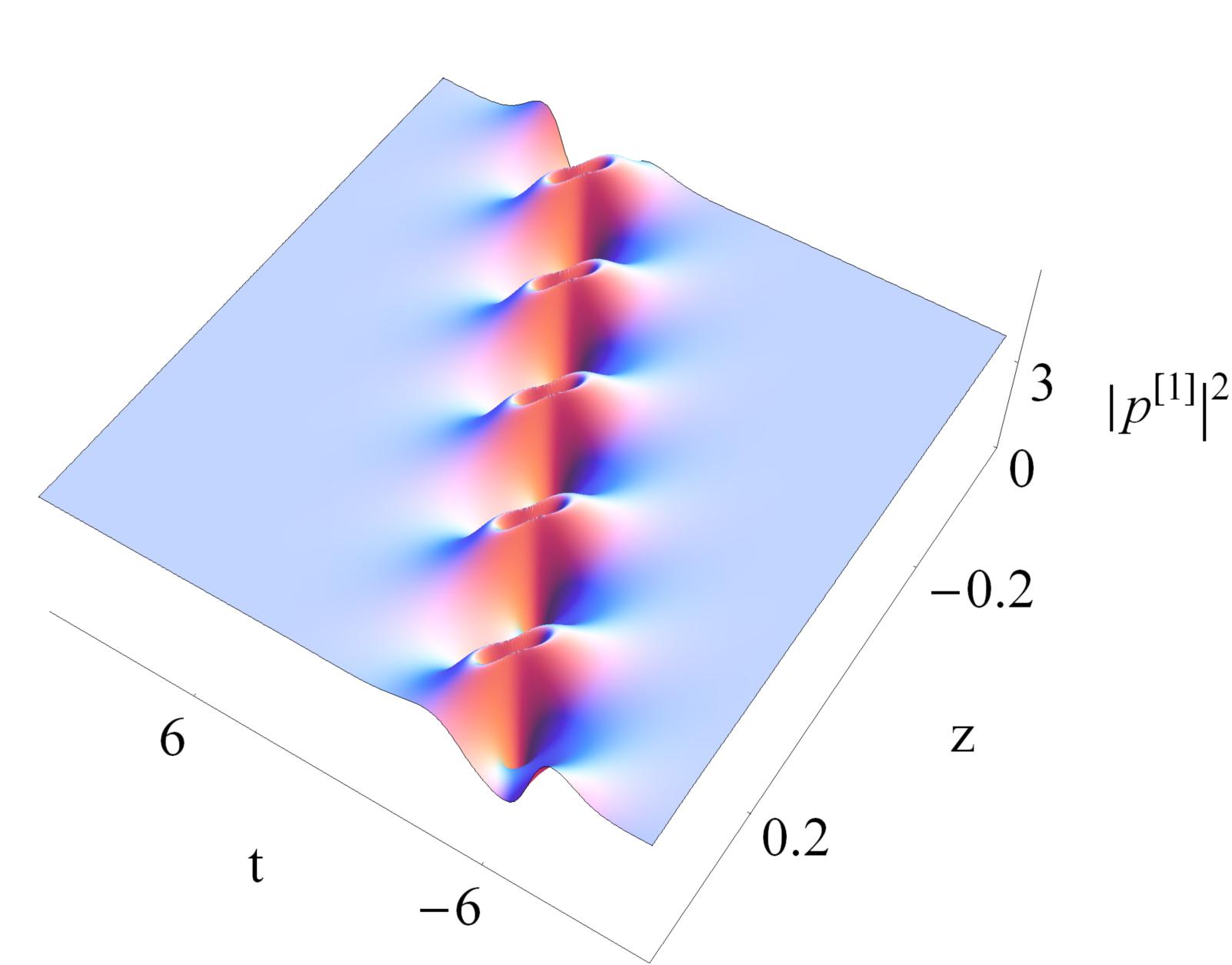
Fig. 1(a)                                               Fig. 1(b)                                                     Fig. 1(c)

Figure 1: First-order breather solution of the GNLS-MB system ($E,p,\eta$) with $d=1,b=2,k_{1}=-k_{2}=1,\omega=\frac{1}{2},\tau=\frac{1}{2}$ and $\lambda_{1}=\lambda_{2}^{\ast}=-1.2+1\,i$

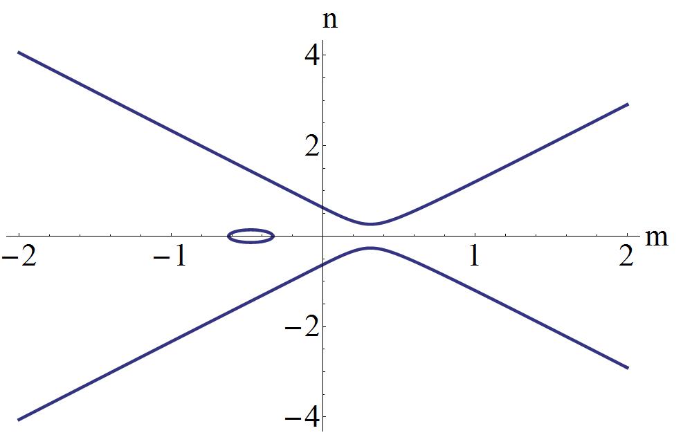
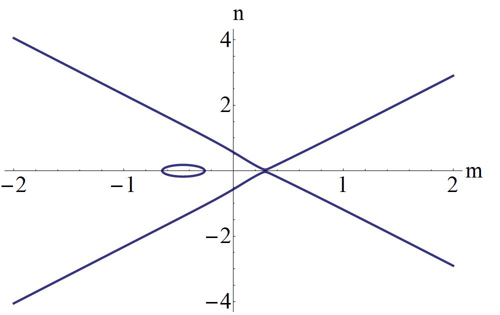
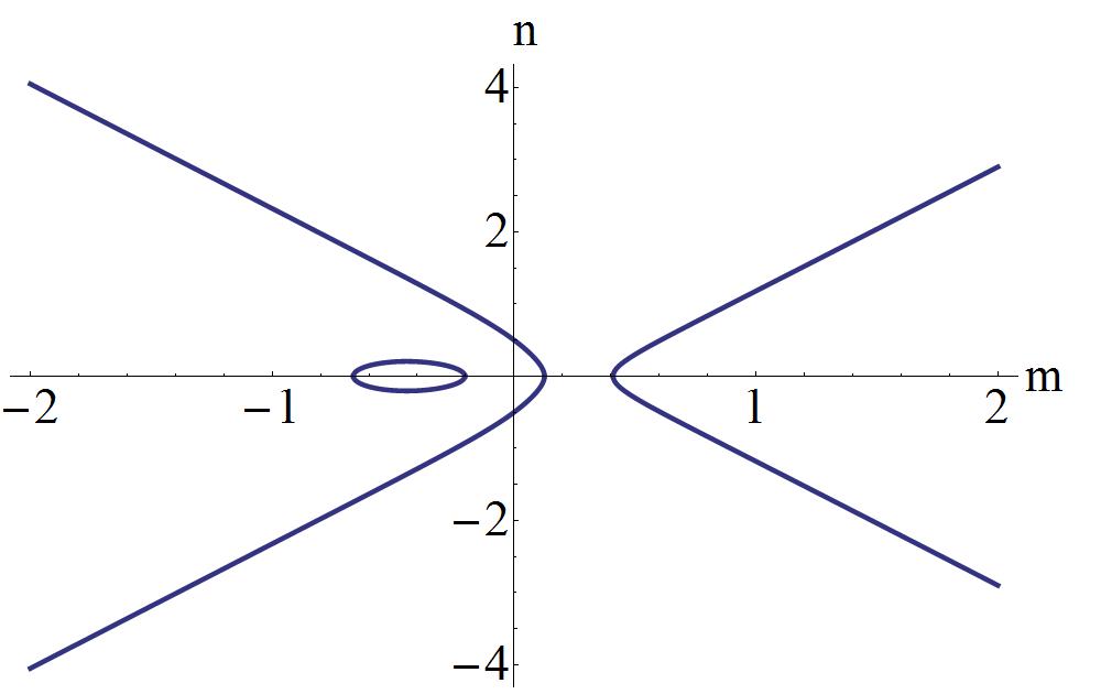
Fig. 2(a)                                             Fig. 2(b)                                            Fig. 2(c)
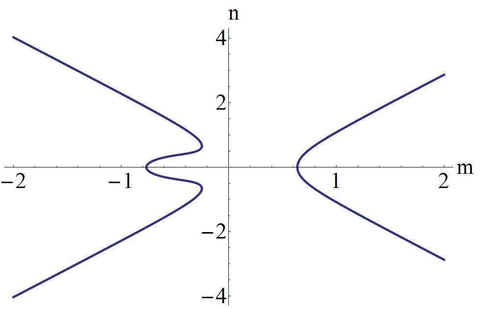
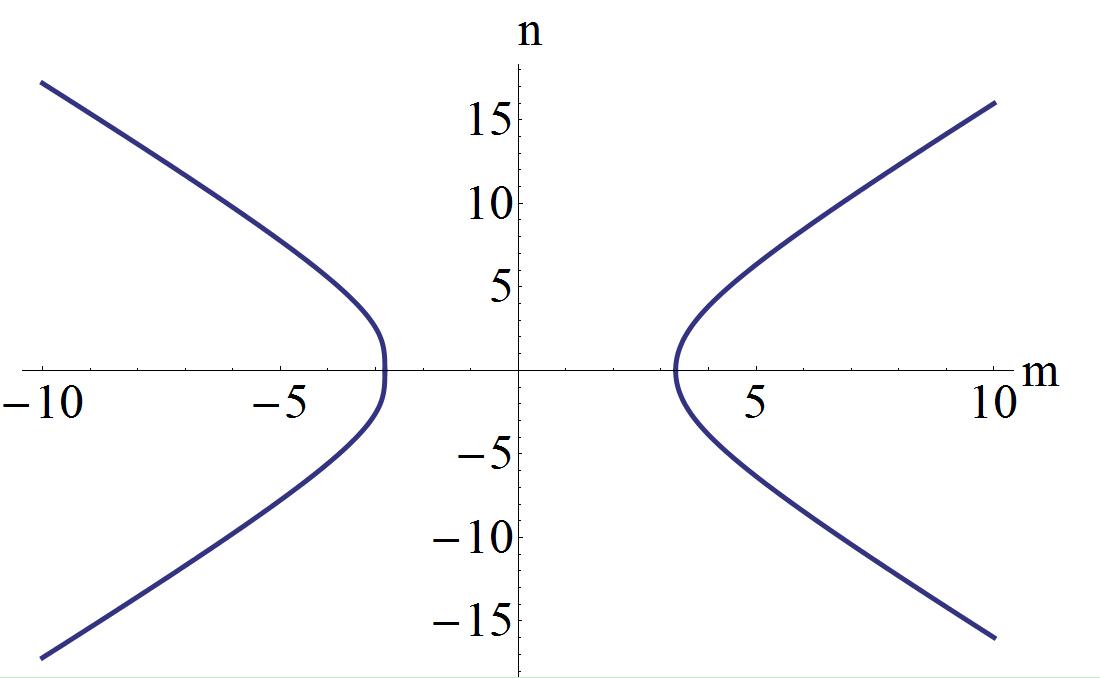
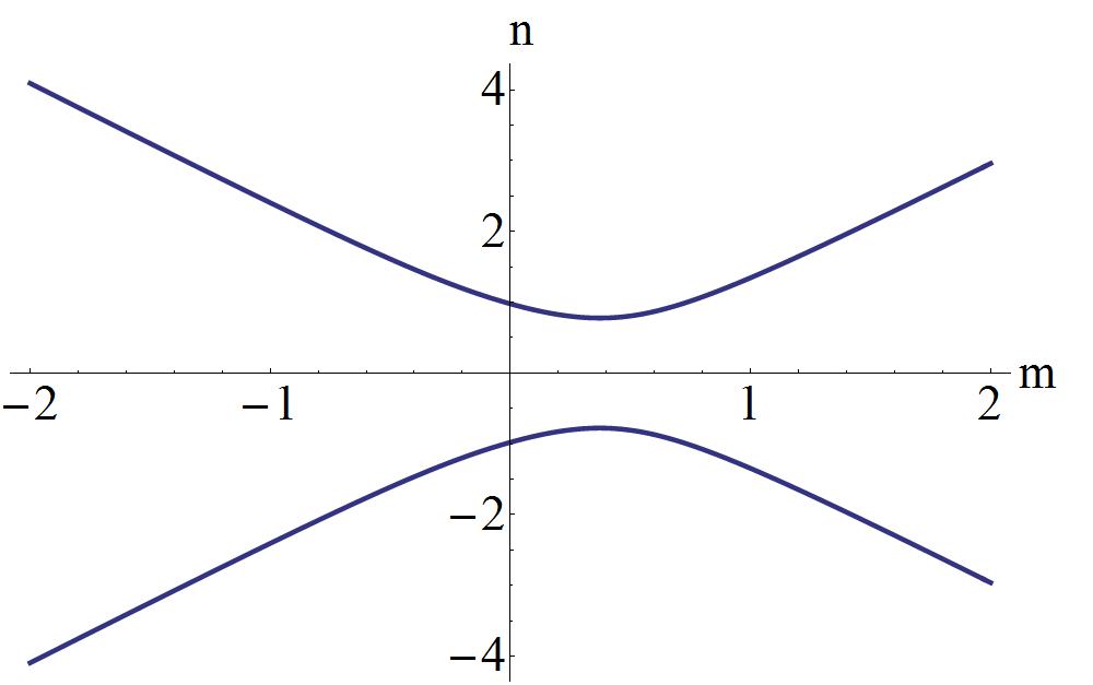
                                                  Fig. 2(d)                                             Fig. 2(e)                                            Fig. 2(f)

Figure 2: Solutions of Eq. (2.3) on a complex plane of $\lambda_{1}=m+n\,i$.$\,d=1,b=2,\omega=\frac{1}{2}$. (a): $\tau=6$, (b): $\tau=3.8$, (c): $\tau=3$, (d):$\tau=1$, (e): $\tau=0.01$, (f): $\tau=-1$.

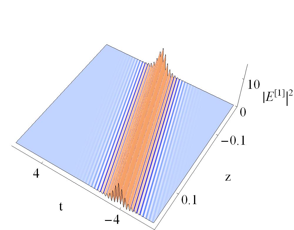
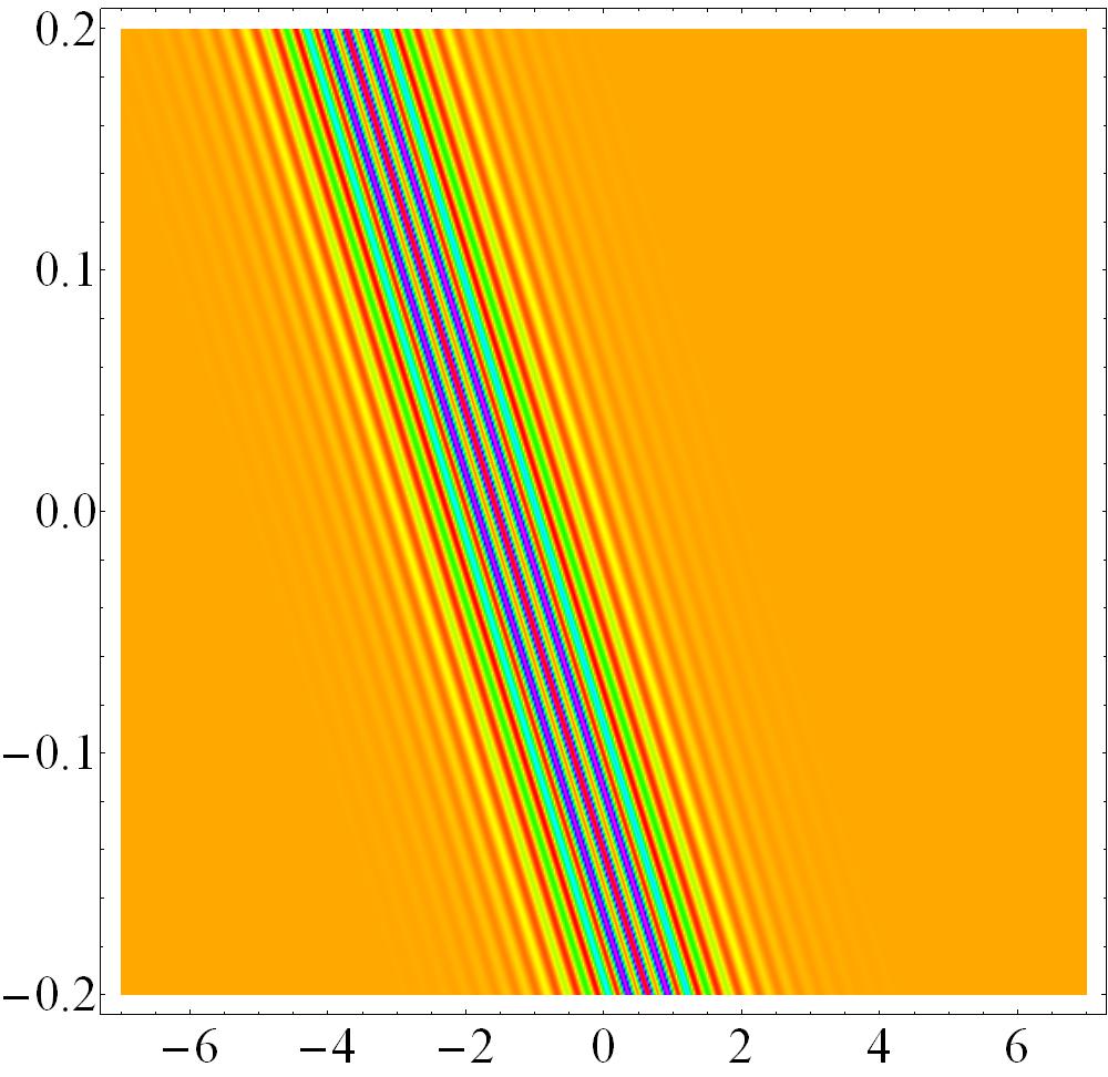
Fig. 3(a)                                             Fig. 3(b)                                                 Fig. 3(c)

Figure 3: A breather transformed into a multi-peak soliton with $d=1,b=2,k_{1}=-k_{2}=1,\omega=\frac{1}{2}$ and $\lambda_{1}=\lambda_{2}^{\ast}=9.6+i$. (b) is the contour plot of (a). (c) is the cross-sectional view of (a) at $z=0$.

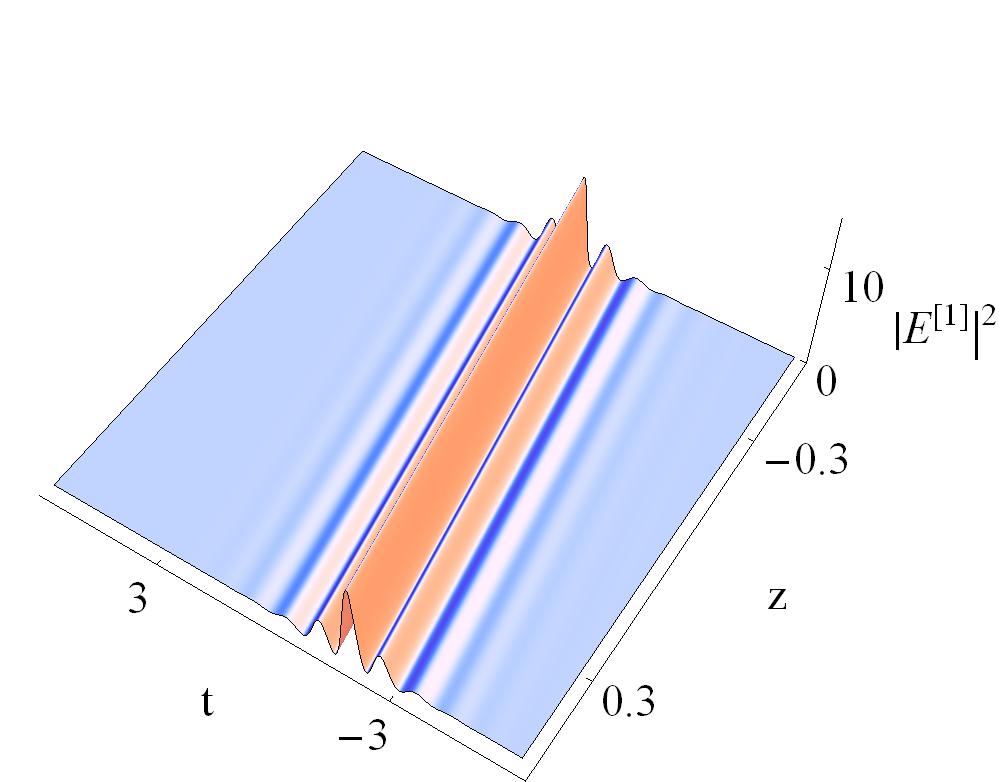
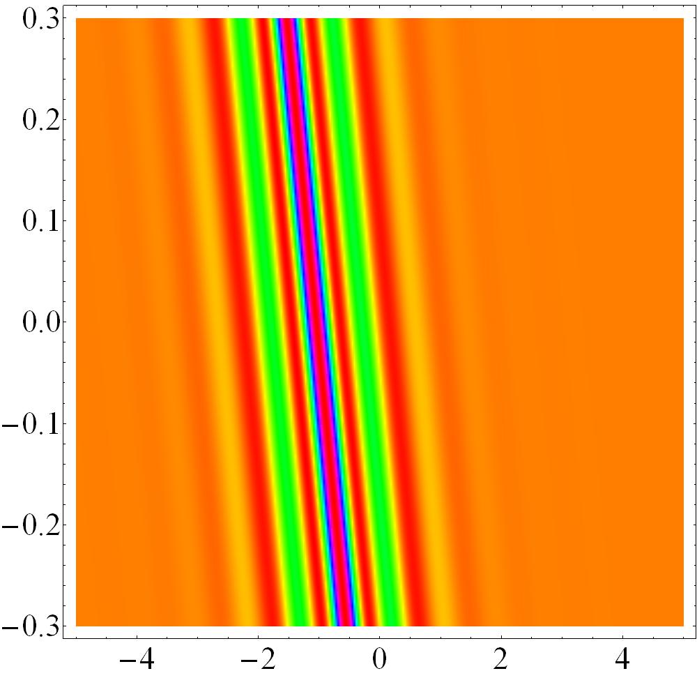
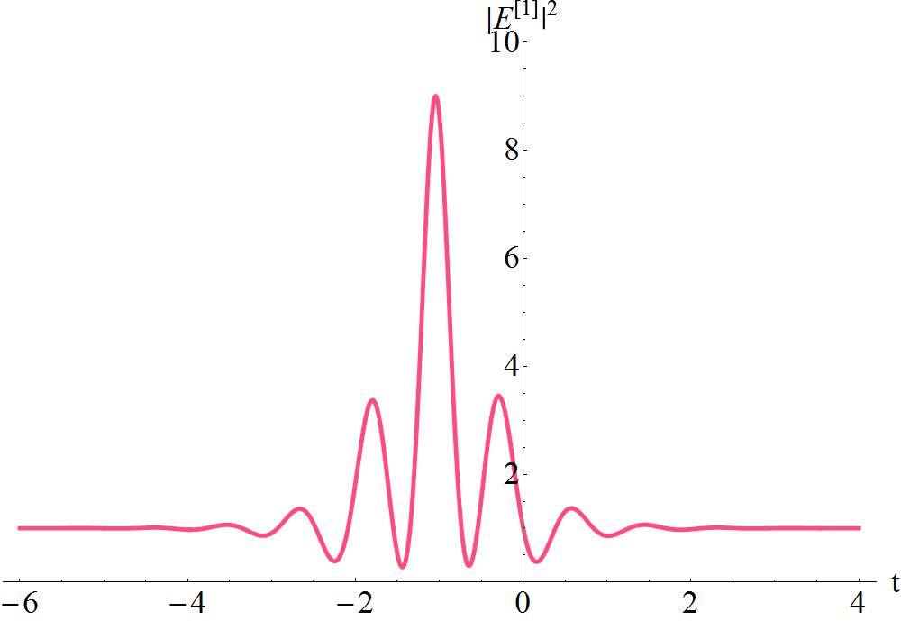
Fig. 4(a)                                             Fig. 4(b)                                                 Fig. 4(c)

Figure 4: A breather transformed into a multi-peak soliton with $d=1,b=2,k_{1}=-k_{2}=1,\omega=\frac{1}{2}$ and $\lambda_{1}=\lambda_{2}^{\ast}=2.5+i$. (b)is the contour plot of (a). (c) is the cross-sectional view of (a) at $z=0$.

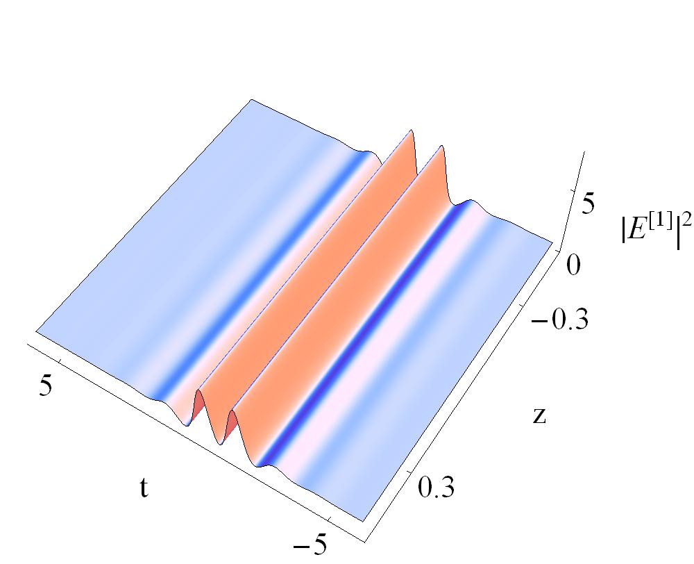
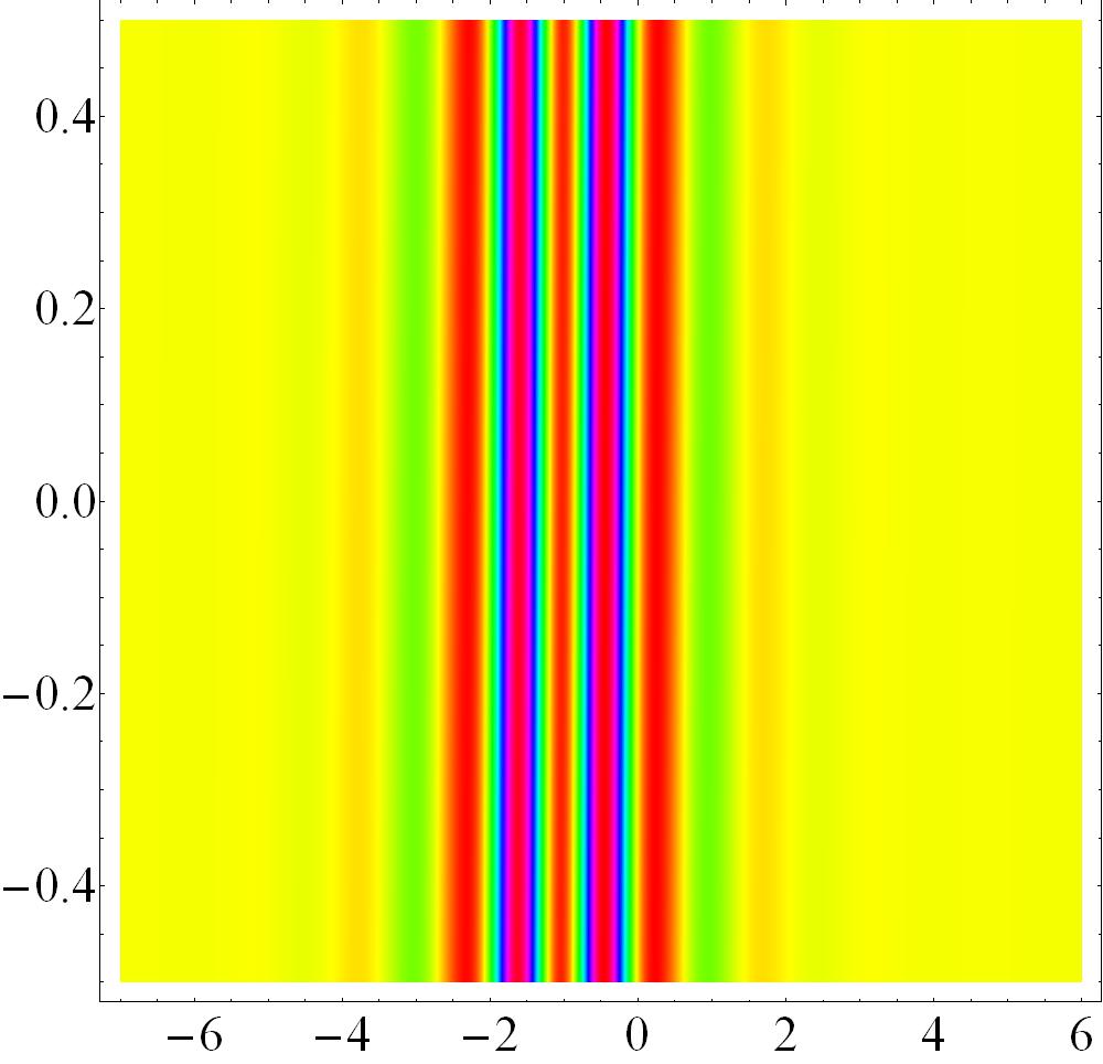
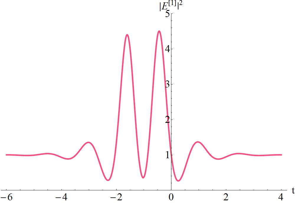
Fig. 5(a)                                             Fig. 5(b)                                                 Fig. 5(c)

Figure 5: A breather transformed into a M-shape soliton with $d=1,b=2,k_{1}=-k_{2}=1,\omega=\frac{1}{2}$ and $\lambda_{1}=\lambda_{2}^{\ast}=0.9+0.8\,i$. (b) is the contour plot of (a). (c) is the cross-sectional view of (a) at $z=0$.

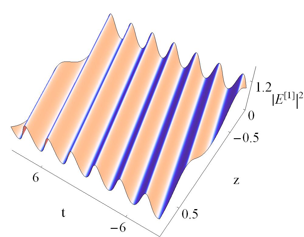
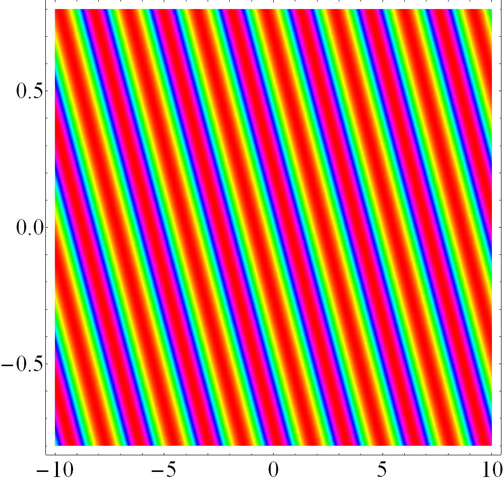
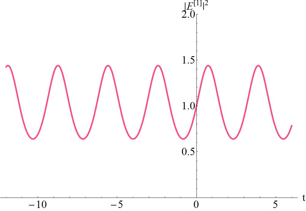
Fig. 6(a)                                             Fig. 6(b)                                                 Fig. 6(c)

Figure 6: A breather transformed into a multi-peak soliton (equal-amplitude) with $d=1,b=2,k_{1}=-k_{2}=1,\omega=\frac{1}{2}$ and $\lambda_{1}=\lambda_{2}^{\ast}=-1-0.1\,i$. (b) is the contour plot of (a). (c) is the cross-sectional view of (a) at $z=0$.

Fig. 7(a)                                             Fig. 7(b)                                                 Fig. 7(c)

Figure 7: A breather transformed into an antidark soliton with $d=1,b=2,k_{1}=k_{2}=1,\omega=\frac{1}{2}$ and $\lambda_{1}=\lambda_{2}^{\ast}=-\frac{1}{2}\,b+1.5\,i$. (b) is the contour plot of (a). (c) is the cross-sectional view of (a) at $z=0$.

Fig. 8(a)                                             Fig. 8(b)                                                 Fig. 8(c)

Figure 8: A breather transformed into period wave with $d=1,b=2,k_{1}=-k_{2}=1,\omega=\frac{1}{2}$ and $\lambda_{1}=\lambda_{2}^{\ast}=-\frac{1}{2}\,b+0.8\,i$. (b) is the contour plot of (a). (c) is the cross-sectional view of (a) at $z=0$.

Fig. 9(a)                                                                  Fig. 9(b)

Figure 9: First-order asymmetric RW solution with $d=1,b=2,k_{1}=-k_{2}=1,\omega=\frac{1}{2},\tau=\frac{1}{2}$ and $\lambda_{1}=\lambda_{2}^{\ast}=-\frac{1}{2}\,b+i\,d$.

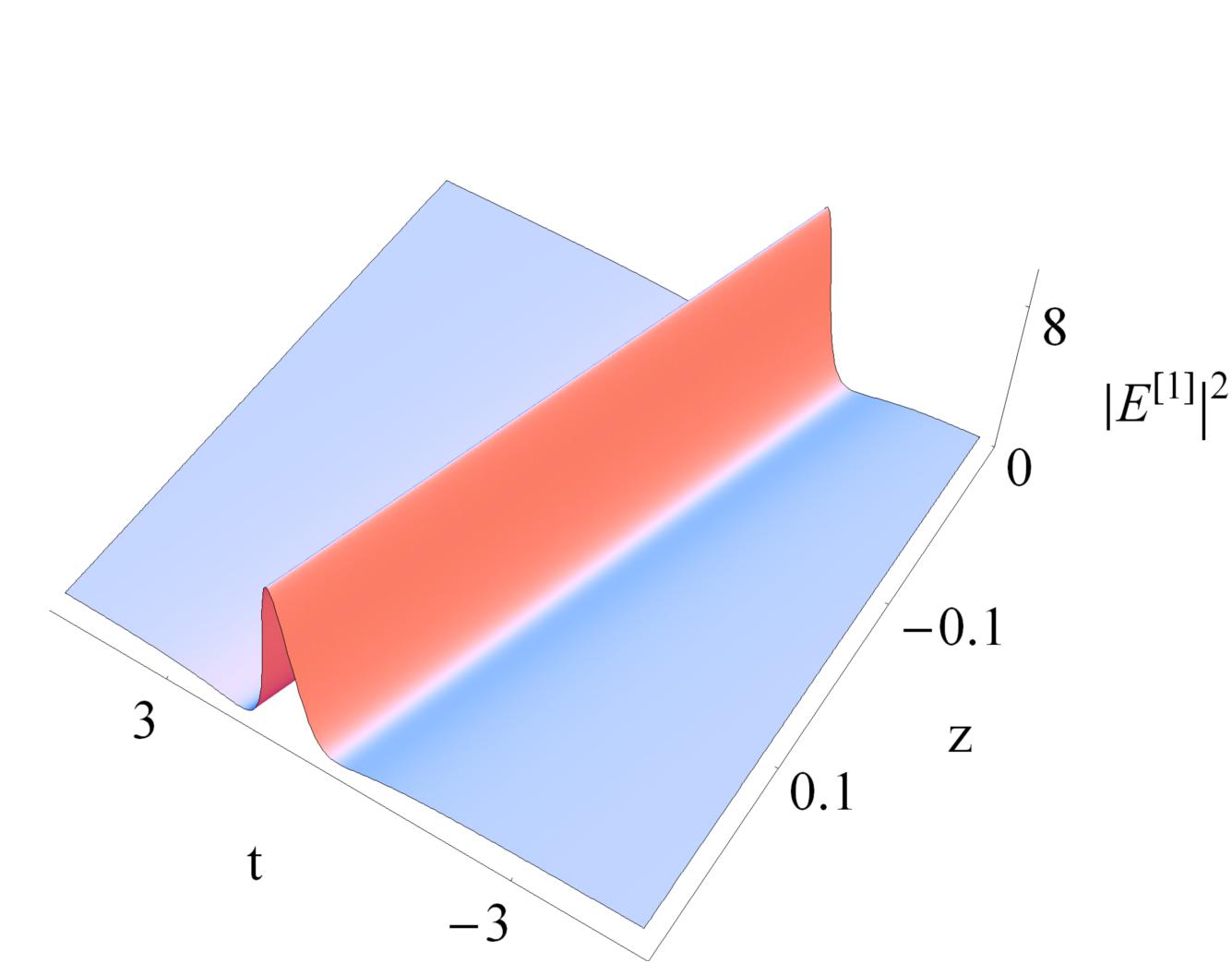
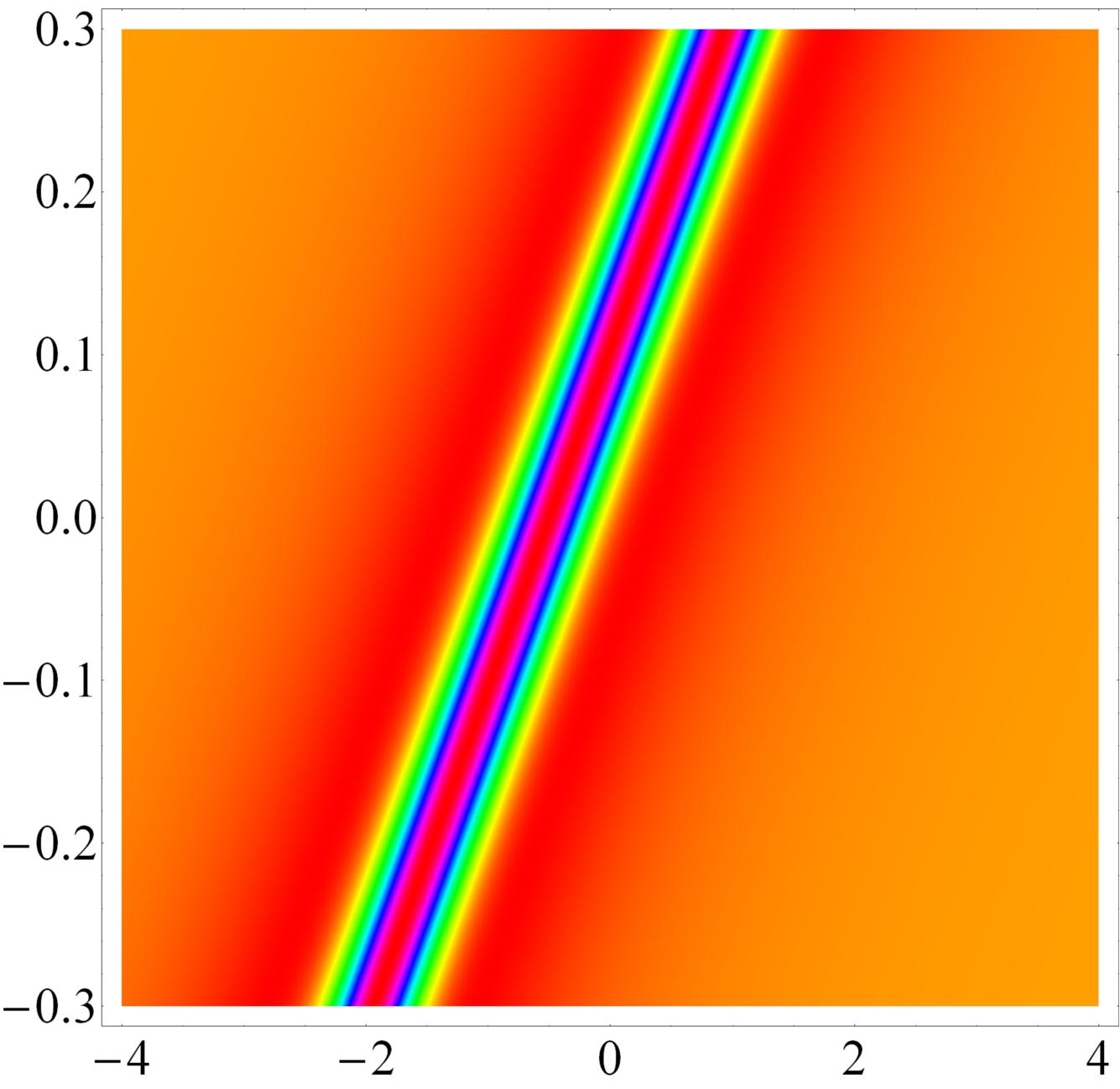
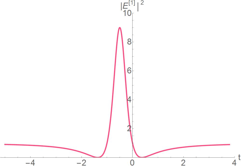
Fig. 10(a)                                             Fig. 10(b)                                                 Fig. 10(c)

Figure 10: An asymmetric RW transformed into a W-shaped soliton with $d=1,b=0,k_{1}=-k_{2}=1,\omega=\frac{1}{2}$ and $\lambda_{0}=-\frac{1}{2}\,b+i\,d$. (b) is the contour plot of (a). (c) is the cross-sectional view of (a) at $z=0$.

References

• (1) Agrawal,  G.P.:  Nonlinear Fiber Optics, Academic Press, San Diego, Calif, USA, 2001.
• (2) Hasegawa, A., Tappert, F.D.: Transmission of stationary nonlinear optical pulses in dispersive dielectric fibers. I. Anomalous dispersion. Appl. Phys. Lett. 23, 142 (1973).
• (3) Porsezian,  K.,  Nakkeeran,  K.:  Optical Soliton Propagation in an Erbium Doped Nonlinear Light Guide with Higher Order Dispersion. Phys. Rev. Lett. 74, 2941 (1995).
• (4) McCall,  S.L.,   Hahn,  E.L.:   Self-Induced Transparency by Pulsed Coherent Light. Phys. Rev. Lett. 18, 908 (1967). G. L. Lamb Jr., Elements of Soliton Theory. New York: Wiley-Intersci; 1980.
• (5) Doktorov,  E.V.,  Vlasov,  R.A.:  Optical Solitons in Media with Resonant and Non-resonant Self-focusing Nonlinearities Opt. Act. 30, 223 (1983).
• (6) Maimistov,  A.I.,  Manykin,  E.A.:  Propagation of ultrashort optical pulses in resonant nonlinear light guides . Sov. Phys. JETP 58, 685 (1983).
• (7) Nakazawa,  M.,  Yamada,  E.,  Kubota,  H.:  Coexistence of self-induced transparency soliton and nonlinear Schrödinger soliton. Phys. Rev. Lett. 66, 2625 (1991).
• (8) Porsezian,  K.,  Mahalingam,  A.,  Sundaram,  P.S.:  Solitons in the system of coupled Hirota-Maxwell-Bloch equations. Chaos, Solitons Fract. 11, 1261 (2000).
• (9) Nakkeeran,  K.:  Optical solitons in erbium doped fibers with higher order effects. Phys. Lett. A 275, 415 (2000).
• (10) Yang,  B.,  Zhang,  W.G.,  Zhang,  H.Q.,  Pei,  S.B.:  Generalized Darboux transformation and rogue wave solutions for the higher-order dispersive nonlinear Schrödinger equation. Phys. Scr. 88, 065004 (2013).
• (11) Ankiewicz,  A.,  Wang,  Y.,  Wabnitz,  S.,  Akhmediev,  N.:  Ext-ended nonlinear Schrödinger equation with higher-order odd and even terms and its rogue wave solutions. Phys. Rev. E 89, 012907 (2014).
• (12) Ankiewicz,  A.,  Akhmediev,  N.:  Higher-order integrable evolution equation and its soliton solutions. Phys. Lett. A 378, 358 (2014).
• (13) Davydova,  T.A.,  Zaliznyak,  Y.A.:  Schrödinger ordinary solitons and chirped solitons: fourth-order dispersive effects and cubic-quintic nonlinearity. Phys. D 156, 260 (2001).
• (14) Li,  L.J.,  Wu,  Z.W.,  Wang,  L.H.,  He,  J.S.:  High-order rogue waves for the Hirota equation. Ann. Phys. 334, 198 (2013).
• (15) Guo,  R.,  Hao,  H.Q.,  Gu,  X.S.:  Modulation Instability, Brea-
thers, and Bound Solitons in an Erbium-Doped Fiber System with Higher-Order Effects. Abstr. Appl. Anal. 2014, 185654 (2014).
• (16) Zhang,  Y.,  Li,  C.Z.,  He,  J.S.:  Rogue waves in a resonant erbium-doped fiber system with higher-order effects. arXiv: 1505.02237.
• (17) Wang,  Q.M.,  Gao,  Y.T.,  Su,  C.Q.,  Zuo,  D.W.:  Solitons, br-
eathers and rogue waves for a higher-order nonlinear Schrödinger CMaxwell CBloch system in an erbium-doped fiber system. Phys. Scr. 90, 105202 (2015).
• (18) Su,  C.Q.,  Gao,  Y.T.,  Xue,  L.,  Yu,  X.: Solitons and Rogue Waves for a Higher-Order Nonlinear Schrödinger-Maxwell-Bloch System in an Erbium-Doped Fiber. Z. Naturforsch. A. 70, 935 (2015).
• (19) Zuo,  D.W.,  Gao,  Y.T.,  Feng,  Y.J.,  Xue,  L.:  Rogue-wave interaction for a higher-order nonlinear Schrödinger-Maxwell-Bloch system in the optical-fiber communication. Nonlinear Dyn. 78, 2309 (2014).
• (20) Li,  J.T.,  Han,  J.Z.,  Du,  Y.D.,  Dai,  C.Q.:  Controllable beha-
viors of Peregrine soliton with two peaks in a birefringent fiber with higher-order effects. Nonlinear Dyn. 82, 1393 (2015).
• (21) Xie,  X.Y.,  Tian,B.,  Sun,  W.R.,  Sun,  Y.:  Rogue-wave soluti-
ons for the Kundu-Eckhaus equation with variable coefficients in an optical fiber. Nonlinear Dyn. 81, 1349 (2015).
• (22) Yang,  Y.Q.,  Wang,  X.,  Yan,  Z.Y.:  Optical temporal rogue waves in the generalized inhomogeneous nonlinear Schrödin-
ger equation with varying higher-order even and odd terms. Nonlinear Dyn. 81, 833 (2015).
• (23) Sun,  W.R.,  Tian,  B.,  Zhen,  H.L.,  Sun,  Y.:  Breathers and ro-
gue waves of the fifth-order nonlinear Schrödinger equation in the Heisenberg ferromagnetic spin chain. Nonlinear Dyn. 81, 725 (2015).
• (24) Meng,  G.Q.,  Qin,  J.L.,  Yu,  G.L.:  Breather and rogue wave solutions for a nonlinear Schrödinger-type system in plasmas. Nonlinear Dyn. 81, 739 (2015).
• (25) Chen,  H.Y.,  Zhu,  H.P.:  Controllable behaviors of spatiotemporal breathers in a generalized variable-coefficient nonlinear Schrödinger model from arterial mechanics and optical fibers. Nonlinear Dyn. 81, 141 (2015).
• (26) Guo,  R.,  Liu,  Y.F.,  Hao,  H.Q.,  Qi,  F.H.:  Coherently coupled solitons, breathers and rogue waves for polarized optical waves in an isotropic medium. Nonlinear Dyn. 80, 1221 (2015).
• (27) Yan,  Z.Y.:  Two-dimensional vector rogue wave excitations and controlling parameters in the two-component Gross-Pitaevskii equations with varying potentials. Nonlinear Dyn. 79, 2515 (2015).
• (28) Zhu,  H.P.:  Spatiotemporal solitons on cnoidal wave backgrounds in three media with different distributed transverse diffraction and dispersion. Nonlinear Dyn. 76, 1651 (2014).
• (29) Yu,  F.J.:  Matter rogue waves and management by external potentials for coupled Gross-Pitaevskii equation. Nonlinear Dyn. 80, 685 (2015).
• (30) Guo,  R.,  Hao,  H.Q.,  Zhang,  L.L.:  Dynamic behaviors of the breather solutions for the AB system in fluid mechanics. Nonlinear Dyn. 74, 701 (2013).
• (31) Kedziora,  D.J.,  Ankiewicz,  A.,  Akhmediev,  N.:  Second-ord-
er nonlinear Schrödinger equation breather solutions in the degenerate and rogue wave limits. Phys. Rev. E 85, 066601 (2012).
• (32) Ren,  Y.,  Yang,  Z.Y.,  Liu,  C.,  Yang,  W.L.:  Different types of nonlinear localized and periodic waves in an erbium-doped fiber system. Phys. Lett. A 379, 45 (2015).
• (33) Chowdury,  A.,  Ankiewicz,  A.,  Akhmediev,  N.:  Moving brea-
thers and breather-to-soliton conversions for the Hirota equation. Proc. R. Soc. A 471, 20150130 (2015).
• (34) Chowdury,  A.,  Kedziora,  D.J.,  Ankiewicz,  A.,  Akhmediev,  N.   :  Breather-to-soliton conversions described by the quintic equation of the nonlinear Schrödinger hierarchy. Phys. Rev. E 91, 032928 (2015).
• (35) Liu, C.,   Yang, Z. Y.,  Zhao L. C.,  Yang, W. L.: Transition, coexistence, and interaction of vector localized waves arising from higher-order effects. Ann. Phys. 362, 130 (2015).
• (36) Liu, C.,  Yang, Z.Y.,  Zhao, L.C.,  Yang, W.L.: State transition induced by higher-order effects and background frequency. Phys. Rev. E 91, 022904 (2015).
• (37) Barashenkov,  I.V.,  Smirnov,  Yu.S.:  Existence and stability chart for the ac-driven, damped nonlinear Schrödinger solitons. Phys. Rev. E 54, 5707 (1996).
• (38) Barashenkov,  I.V.,  Zemlyanaya,  E.V.,  Travelling solitons in the externally driven nonlinear Schrödinger equation. J. Phys. A: Math. Theor. 44, 465211 (2011).
• (39) Kivshar,  Yu.S.:  Nonlinear dynamics near the zero-dispersion point in optical fibers. Phys. Rev. A 43, 1677 (1991).
• (40) Kivshar,  Yu.S.,  Afanasjev,  V.V.:  Dark optical solitons with reverse-sign amplitude. Phys. Rev. A 44, 1446(R) (1991).
• (41) He,  J.S.,  Xu,  S.W.,  Ruderman,  M.S.,  Erdelyi,  R.:  State Tr-
ansition Induced by Self-Steepening and Self Phase-Modulation. Chin. Phys. Lett. 31, 010502 (2014).
• (42) He,  J.S.,  Xu,  S.W.,  Cheng,  Y.:  The rational solutions of the mixed nonlinear Schrödinger equation. AIP Advances 5, 017105 (2015).
Refer to caption
Refer to caption
Refer to caption