Twisted Interferometry: the topological perspective

Abstract

Three manifold topology is used to analyze the effect of anyonic interferometers in which the probe anyons’ path along an arm crosses itself, leading to a “twisted” or braided space-time trajectory for the probe anyons. In the case of Ising non-Abelian anyons, twisted interferometry is shown to be able to generate a topologically protected $\pi/8$-phase gate, which cannot be generated from quasiparticle braiding.

, , ,

1 Introduction

Anyonic interferometry [Bonderson07b, Bonderson07c] is a powerful tool for processing topological quantum information [Kitaev03, Freedman98, Preskill98, Freedman02a, Freedman02b, Freedman03b, Nayak08]. Its ability to non-demolitionally measure the collective anyonic charge of a group of (non-Abelian) anyons, without decohering their internal state, allows it to generate braid operators [Bonderson08a, Bonderson08b], generate entangling gates [Bravyi00, Bravyi06, BondersonWIP, Levaillant2015d], and change between different qubit encodings [BondersonWIP, Levaillant2015d]. Anyonic interferometry has been the focus of myriad experimental proposals [Chamon97, Fradkin98, DasSarma05, Stern06a, Bonderson06a, Bonderson06b, Fidkowski07c, Ardonne08a, Bishara08a, Bishara09, Akhmerov09a, Fu09a, Bonderson11b, Grosfeld11a] and efforts to physically implement them [Camino05a, Willett09a, Willett09b, McClure12, An11, Willett12a, Willett12b]. As powerful as anyonic interferometry may be, its potential capabilities have yet to be fully understood. In this paper, we propose and analyze a novel implementation of anyonic interferometry that we call “twisted interferometry,” which can significantly augment its potential capabilities.

One of the primary practical motivations for studying twisted interferometry is that it could be used with anyons of the Ising TQFT to generate “magic states,” as we will demonstrate. This is significant because, if one only has the ability to perform braiding operations and untwisted anyonic interferometry measurements for Ising anyons, then one can only generate the Clifford group operations, which is not computationally universal and, in fact, can be efficiently simulated on a classical computer [Gottesman98]. However, if one supplements these operations with magic states, then one can also generate $\pi/8$-phase gates, which results in a computationally universal gate set [Boykin99].

The application of twisted interferometry to generating the $\pi/8$-phase gate for Ising anyons is the latest link in a chain of ideas [Bravyi00-unpublished, Freedman06a, FNW05b, Bonderson10], originating with the unpublished work of Bravyi and Kitaev, for generating a topologically-protected computational universal gate set from the Ising TQFT by utilizing topological operations. The concept and analysis of twisted interferometry is new, but closely connected to these ideas, which stem from the concept of Dehn surgery on $3$-manifolds. As we will discuss in detail, anyonic interferometry: 1) projectively measures the topological charge inside $\gamma$, and 2) decoheres the anyonic entanglement between the subsystems inside and outside the interference loop $\gamma$ [Bonderson07a]. Both operations have a 3D topological interpretation in the context of Chern-Simons theory or, more generally, axiomatic (2+1)D topological quantum field theories (TQFTs). We learned from Witten [Witten89] that all low energy properties of systems governed by a TQFT can be calculated in a Euclidean signature diagrammatic formalism called unitary modular tensor categories (UMTC). This suggests [Freedman06a, FNW05b] that the choice of interference loop $\gamma$ should not be restricted to a simple space-like loop in a spatial slice ${\mathbb{R}}^{2}\subset{\mathbb{R}}^{2}\times$time, as is the typical design for an interferometer, but rather $\gamma$ might be a general simple closed curve of space-time. Twisted interferometry explores this direction by allowing the probe anyons’ path through the arms of the interferometer to be self-crossing in ${\mathbb{R}}^{2}$ (so $\gamma$ is immersed in mathematical terminology). We give a general procedure for analyzing interferometers of this kind. In the restricted case of the Ising TQFT, we describe a twisted interferometer which would be capable of producing magic states.

Our strategy is: 1) to start with the UMTC calculation [Bonderson07b, Bonderson07c] which lays bare the asymptotic behavior of the simplest anyonic Mach-Zehnder interferometer (and serves as a model for Fabrey-Pérot type interferometers in the weak tunneling limit); 2) describe this behavior in an equivalent topological language; and 3) exploit the general covariance inherent in the topological description.

The concrete calculation using the machinery of UMTCs is carried out in a companion paper [Bonderson13b], which also focuses on possible physical implementations of twisted interferometers. The analysis of the companion paper agrees with the topological argument presented here and both show how magic state production is achieved when specialized to the Ising theory.

2 What an Anyonic Interferometer Does in Two Different Languages

We recall the bare bones of anyonic interferometry in a general anyonic context (as developed in [Bonderson07b, Bonderson07c]; see [Bonderson13b] for notational clarification and calculational details).

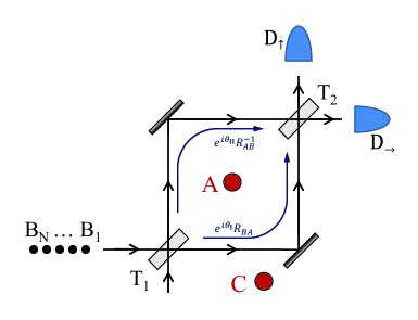
Figure 2.1: An idealized Mach-Zehnder interferometer for an anyonic system, where $T_{j}$ are beam splitters. The target anyons (collectively denoted $A$) in the central region share entanglement only with the anyon(s) $C$ outside this region. A beam of probe anyons $B_{1},\ldots,B_{N}$ is sent through the interferometer and detected at one of the two possible outputs by $D_{s}$.

The target anyon $A$ may be a composite of several quasiparticles (anyons), so it is not necessarily in an eigenstate of charge. In the simplest case, which we treat, the probe quasiparticles $B$ are assumed to be uncorrelated, identical, and simple (not composites). In fact, to make the source standard and uncorrelated, the probes will be independently drawn from the vacuum together with an antiparticle (topological charge conjugate anyon), which is then discarded and mathematically “traced out.” We will simplify the discussion in this paper by also assuming the probe has definite topological charge values $B=b$, but the generalization is straightforward. Coming from the left, probe anyon $B_{i}$ encounters first beam splitter $T_{1}$, and then $T_{2}$. The corresponding transition matrices are:

$$T_{j}=\left[\begin{array}[]{cc}t_{j}&r_{j}^{\ast}\\ r_{j}&-t_{j}^{\ast}\end{array}\right].$$ (2.1)

The unitary operator representing a probe anyon passing through the interferometer is given by

$$U=T_{2}\Sigma T_{1}$$ (2.2)

$$\Sigma=\left[\begin{array}[]{cc}0&e^{i\theta_{\text{II}}}R_{AB}^{-1}\\ e^{i\theta_{\text{I}}}R_{BA}&0\end{array}\right].$$ (2.3)

This can be written diagrammatically as

$$\pspicture[missing](-5.69054pt,0.0pt)(28.45274pt,28.45274pt)\rput[tl](0.0pt,0.0pt){$B_{s^{\prime}}$}\rput[tl](0.0pt,34.14328pt){$A$}\rput[tl](24.18483pt,34.14328pt){$B_{s}$}\rput[tl](24.18483pt,0.0pt){$A$}{\psset{linewidth=0.9pt}\psline(11.38109pt,0.0pt)(11.38109pt,6.82864pt)}{\psset{linewidth=0.9pt}\psline(22.19313pt,0.0pt)(22.19313pt,6.82864pt)}{\psset{linewidth=0.9pt}\psline(11.38109pt,22.19313pt)(11.38109pt,28.45274pt)}{\psset{linewidth=0.9pt}\psline(22.19313pt,22.19313pt)(22.19313pt,28.45274pt)}\rput[bl](8.25128pt,6.82864pt){{\psframebox{$U$}}}\endpspicture=e^{i\theta_{\text{I}}}\left[\begin{array}[]{cc}t_{1}r_{2}^{\ast}&r_{1}^{\ast}r_{2}^{\ast}\\ -t_{1}t_{2}^{\ast}&-r_{1}^{\ast}t_{2}^{\ast}\end{array}\right]_{s,s^{\prime}}\pspicture[missing](-5.69054pt,0.0pt)(35.56592pt,28.45274pt)\psset{linewidth=0.9pt,linecolor=black,arrowscale=1.5,arrowinset=0.15}{\psline(26.17651pt,2.84526pt)(5.69054pt,28.45274pt)}{\psline{->}(26.17651pt,2.84526pt)(7.96677pt,25.60747pt)}{\psline(7.96677pt,2.84526pt)(28.45274pt,28.45274pt)}{\psset{border=2pt}\psline{->}(7.96677pt,2.84526pt)(26.17651pt,25.60747pt)}\rput[tl]{0.0}(-5.69054pt,5.69054pt){$B$}\rput[tr]{0.0}(35.56592pt,5.69054pt){$A$}\endpspicture+e^{i\theta_{\text{II}}}\left[\begin{array}[]{cc}r_{1}t_{2}&-t_{1}^{\ast}t_{2}\\ r_{1}r_{2}&-t_{1}^{\ast}r_{2}\end{array}\right]_{s,s^{\prime}}\pspicture[missing](-5.69054pt,0.0pt)(35.56592pt,28.45274pt)\psset{linewidth=0.9pt,linecolor=black,arrowscale=1.5,arrowinset=0.15}{\psline{->}(7.96677pt,2.84526pt)(26.17651pt,25.60747pt)}{\psline(7.96677pt,2.84526pt)(28.45274pt,28.45274pt)}{\psline(26.17651pt,2.84526pt)(5.69054pt,28.45274pt)}{\psset{border=2pt}\psline{->}(26.17651pt,2.84526pt)(7.96677pt,25.60747pt)}\rput[tl]{0.0}(-5.69054pt,5.69054pt){$B$}\rput[tr]{0.0}(35.56592pt,5.69054pt){$A$}\endpspicture,$$ (2.4)

where we introduce the notation of writing the directional index $s$ of the probe quasiparticle as a subscript on its anyonic (topological) charge label, e.g. $B_{s}$. The anyonic state complementary to the region being probed will be denoted by $C$ (and later by two disjoint sectors $C_{1}$ and $C_{2}$).

The passage of a single probe $B$ transforms the density matrix $\rho^{AC}$ for both system and environment by

$$\rho^{AC}\mapsto\rho^{AC}\left(s\right)=\frac{1}{\Pr\left(s\right)}\widetilde{\text{Tr}}_{B}\left[\Pi_{s}VU\left(\rho^{B}\otimes\rho^{AC}\right)U^{\dagger}V^{\dagger}\Pi_{s}\right],$$ (2.5)

where $\widetilde{\text{Tr}}$ is the “quantum trace,” $V$ represents braiding, and

$$\text{Pr}(s)=\widetilde{\text{Tr}}[\Pi_{s}VU\rho U^{\dagger}V^{\dagger}]$$ (2.6)

is the probability of measurement outcome $s$. The effect of this superoperator can be computed by considering the action on the $\rho^{AC}$ density matrix’s basis elements, which is expressed diagrammatically by

$$\psscalebox{.75}{\pspicture[missing](5.69054pt,-88.20349pt)(113.81097pt,91.04877pt)\small{\psset{linewidth=0.9pt,linecolor=black,border=0}\psframe(17.07164pt,25.60747pt)(48.36966pt,39.83383pt)}{\psset{linewidth=0.9pt,linecolor=black,border=0}\psframe(17.07164pt,-25.60747pt)(48.36966pt,-39.83383pt)}\rput[bl]{0.0}(28.45274pt,28.73726pt){$U$}\rput[tl]{0.0}(27.0301pt,-27.59915pt){$U^{{\dagger}}$}\psset{linewidth=0.9pt,linecolor=black,arrowscale=1.5,arrowinset=0.15}{\psline(22.76219pt,-39.83383pt)(22.76219pt,-79.66768pt)}{\psline(22.76219pt,39.83383pt)(22.76219pt,79.66768pt)}{\psline(22.76219pt,25.60747pt)(22.76219pt,-25.60747pt)}{\psset{linewidth=0.9pt,linecolor=black,border=0pt}\psarc(42.67911pt,25.60747pt){19.91692pt}{-60.0}{0.0}}{\psset{linewidth=0.9pt,linecolor=black,arrows=->,arrowscale=1.4,arrowinset=0.15}\psarc{->}(42.67911pt,25.60747pt){19.91692pt}{-60.0}{-10.0}}{\psset{linewidth=0.9pt,linecolor=black,border=0pt}\psarc(62.59602pt,25.60747pt){19.91692pt}{180.0}{240.0}}{\psset{linewidth=0.9pt,linecolor=black,arrows=<-,arrowscale=1.4,arrowinset=0.15}\psarc{<-}(62.59602pt,25.60747pt){19.91692pt}{190.0}{240.0}}{\psset{linewidth=0.9pt,linecolor=black,border=0pt}\psarc(42.67911pt,-25.60747pt){19.91692pt}{0.0}{60.0}}{\psset{linewidth=0.9pt,linecolor=black,arrows=->,arrowscale=1.4,arrowinset=0.15}\psarc{->}(42.67911pt,-25.60747pt){19.91692pt}{0.0}{35.0}}{\psset{linewidth=0.9pt,linecolor=black,border=0pt}\psarc(62.59602pt,-25.60747pt){19.91692pt}{120.0}{180.0}}{\psset{linewidth=0.9pt,linecolor=black,arrows=<-,arrowscale=1.4,arrowinset=0.15}\psarc{<-}(62.59602pt,-25.60747pt){19.91692pt}{145.0}{180.0}}{\psset{linewidth=0.9pt,linecolor=black,border=0pt}\psarc(54.06021pt,36.98856pt){11.38109pt}{90.0}{170.0}}{\psset{linewidth=0.9pt,linecolor=black,border=0pt}\psarc(54.06021pt,-36.98856pt){11.38109pt}{190.0}{270.0}}{\psline(54.06021pt,48.36966pt)(71.13185pt,48.36966pt)}{\psline(54.06021pt,-48.36966pt)(71.13185pt,-48.36966pt)}{\psset{linewidth=0.9pt,linecolor=black,border=0pt}\psarc(71.13185pt,59.75075pt){11.38109pt}{-90.0}{0.0}}{\psset{linewidth=0.9pt,linecolor=black,border=0pt}\psarc(71.13185pt,-59.75075pt){11.38109pt}{0.0}{90.0}}{\psset{linewidth=0.9pt,linecolor=black,border=0}\psframe(73.97713pt,59.75075pt)(91.04877pt,73.97713pt)}{\psset{linewidth=0.9pt,linecolor=black,border=0}\psframe(73.97713pt,-59.75075pt)(91.04877pt,-73.97713pt)}\rput[bl]{0.0}(76.8224pt,62.02698pt){$\Pi_{s}$}\rput[bl]{0.0}(76.8224pt,-71.70091pt){$\Pi_{s}$}{\psset{linewidth=0.9pt,linecolor=black,border=0pt}\psarc(93.89404pt,73.97713pt){11.38109pt}{0.0}{180.0}}{\psset{linewidth=0.9pt,linecolor=black,border=0pt}\psarc(93.89404pt,-73.97713pt){11.38109pt}{-180.0}{0.0}}{\psline(105.27515pt,73.97713pt)(105.27515pt,-73.97713pt)}{\psline(52.63757pt,-8.53581pt)(52.63757pt,8.53581pt)}{\psset{border=2pt}\psline(62.59602pt,-25.60747pt)(62.59602pt,-79.66768pt)}{\psset{border=2pt}\psline(62.59602pt,25.60747pt)(62.59602pt,79.66768pt)}{\psline{->}(22.76219pt,-79.66768pt)(22.76219pt,-59.75075pt)}{\psline{->}(22.76219pt,-25.60747pt)(22.76219pt,3.41432pt)}{\psline{->}(22.76219pt,39.83383pt)(22.76219pt,68.28658pt)}{\psline{->}(62.59602pt,-79.66768pt)(62.59602pt,-59.75075pt)}{\psline{->}(62.59602pt,39.83383pt)(62.59602pt,68.28658pt)}{\psline{->}(105.27515pt,11.38109pt)(105.27515pt,-2.84526pt)}{\psline{->}(54.06021pt,48.08513pt)(57.47453pt,48.65419pt)}{\psline{<-}(51.21494pt,-48.08513pt)(57.47453pt,-48.36966pt)}{\psline{->}(52.63757pt,-8.53581pt)(52.63757pt,3.41432pt)}\rput[bl]{0.0}(19.91692pt,82.51295pt){$a$}\rput[tl]{0.0}(19.91692pt,-79.66768pt){$a^{\prime}$}\rput[bl]{0.0}(59.75075pt,82.51295pt){$c$}\rput[tl]{0.0}(59.75075pt,-79.66768pt){$c^{\prime}$}\rput[bl]{0.0}(8.53581pt,-2.84526pt){$b_{\shortrightarrow}$}\rput[bl]{0.0}(109.54306pt,-2.84526pt){$b_{s}$}\rput[bl]{0.0}(44.10175pt,-5.69054pt){$f$}\rput[bl]{0.0}(36.13498pt,11.38109pt){$a$}\rput[bl]{0.0}(34.99687pt,-17.07164pt){$a^{\prime}$}\scriptsize\rput[bl]{0.0}(50.07683pt,14.22636pt){$\mu$}\rput[bl]{0.0}(48.65419pt,-19.91692pt){$\mu^{\prime}$}\endpspicture}$$ (2.7)

For the outcome $s=\shortrightarrow$, this may be expanded as

$$\sum\limits_{\left(e,\alpha,\beta\right)}\left[\left(F_{a^{\prime}c^{\prime}}^{ac}\right)^{-1}\right]_{\left(f,\mu,\mu^{\prime}\right)\left(e,\alpha,\beta\right)}$$ (2.8)

$$\times\left\{\left|t_{1}\right|^{2}\left|r_{2}\right|^{2}\pspicture[missing](0.0pt,-34.14328pt)(54.06021pt,32.72064pt)\small{\psset{linewidth=0.9pt,linecolor=black,border=0}\psellipse(33.85876pt,0.0pt)(5.12149pt,11.38109pt)}\psset{linewidth=0.9pt,linecolor=black,arrowscale=1.4,arrowinset=0.15}{\psline{>-}(30.72896pt,-8.53581pt)(29.30632pt,-2.84526pt)}\psset{linewidth=0.9pt,linecolor=black,arrowscale=1.5,arrowinset=0.15}{\psline(9.95845pt,-22.05087pt)(9.95845pt,22.05087pt)}{\psline{>-}(9.95845pt,8.53581pt)(9.95845pt,17.07164pt)}{\psline{<-}(9.95845pt,-8.53581pt)(9.95845pt,-17.07164pt)}{\psline(44.10175pt,-22.05087pt)(44.10175pt,22.05087pt)}{\psline{>-}(44.10175pt,8.53581pt)(44.10175pt,17.07164pt)}{\psline{<-}(44.10175pt,-8.53581pt)(44.10175pt,-17.07164pt)}{\psline(32.1516pt,-0.85358pt)(44.10175pt,-2.84526pt)}{\psset{border=2pt}\psline(32.1516pt,-0.85358pt)(42.39458pt,-2.56075pt)}{\psline{-<}(9.95845pt,2.84526pt)(23.61577pt,0.56905pt)}{\psline(9.95845pt,2.84526pt)(26.17651pt,0.14226pt)}\rput[bl]{0.0}(7.11317pt,24.89615pt){$a$}\rput[bl]{0.0}(41.25647pt,24.89615pt){${c}$}\rput[bl]{0.0}(7.11317pt,-30.58669pt){$a^{\prime}$}\rput[bl]{0.0}(41.25647pt,-30.58669pt){${c^{\prime}}$}\rput[br]{0.0}(25.60747pt,5.69054pt){$e$}\rput[br]{0.0}(27.59915pt,-14.79543pt){$b$}\scriptsize\rput[br]{0.0}(7.96677pt,1.42262pt){$\alpha$}\rput[br]{0.0}(51.78398pt,-7.11317pt){$\beta$}\endpspicture\right.+t_{1}r_{1}^{\ast}r_{2}^{\ast}t_{2}^{\ast}e^{i\left(\theta_{\text{I}}-\theta_{\text{II}}\right)}\pspicture[missing](-7.11317pt,-28.45274pt)(51.21494pt,38.4112pt)\small{\psset{linewidth=0.9pt,linecolor=black,border=0}\psellipse(9.95845pt,17.07164pt)(11.38109pt,5.12149pt)}\psset{linewidth=0.9pt,linecolor=black,arrowscale=1.4,arrowinset=0.15}{\psline{->}(2.84526pt,20.62823pt)(8.53581pt,21.9086pt)}\psset{linewidth=0.9pt,linecolor=black,arrowscale=1.5,arrowinset=0.15}{\psline(9.95845pt,-17.07164pt)(9.95845pt,19.63239pt)}{\psline(9.95845pt,23.9003pt)(9.95845pt,27.0301pt)}{\psset{border=3pt}\psline{>-}(9.95845pt,8.53581pt)(9.95845pt,17.07164pt)}{\psline{<-}(9.95845pt,-8.53581pt)(9.95845pt,-17.07164pt)}{\psline(38.4112pt,-17.07164pt)(38.4112pt,27.0301pt)}{\psline{>-}(38.4112pt,8.53581pt)(38.4112pt,17.07164pt)}{\psline{<-}(38.4112pt,-8.53581pt)(38.4112pt,-17.07164pt)}{\psline(9.95845pt,2.84526pt)(38.4112pt,-2.84526pt)}{\psline{->}(38.4112pt,-2.84526pt)(19.91692pt,0.85358pt)}\rput[bl]{0.0}(7.11317pt,29.87537pt){$a$}\rput[bl]{0.0}(35.56592pt,29.87537pt){${c}$}\rput[bl]{0.0}(7.11317pt,-25.60747pt){$a^{\prime}$}\rput[bl]{0.0}(35.56592pt,-25.60747pt){${c^{\prime}}$}\rput[br]{0.0}(27.0301pt,3.69885pt){$e$}\rput[br]{0.0}(-1.42262pt,19.91692pt){$b$}\scriptsize\rput[br]{0.0}(7.96677pt,1.42262pt){$\alpha$}\rput[br]{0.0}(46.09343pt,-7.11317pt){$\beta$}\endpspicture$$

$$+t_{1}^{\ast}r_{1}t_{2}r_{2}e^{-i\left(\theta_{\text{I}}-\theta_{\text{II}}\right)}\pspicture[missing](-7.11317pt,-39.83383pt)(51.21494pt,28.45274pt)\small{\psset{linewidth=0.9pt,linecolor=black,border=0}\psellipse(9.95845pt,-17.07164pt)(11.38109pt,5.12149pt)}\psset{linewidth=0.9pt,linecolor=black,arrowscale=1.4,arrowinset=0.15}{\psline{-<}(1.99168pt,-20.3437pt)(7.68224pt,-21.62408pt)}\psset{linewidth=0.9pt,linecolor=black,arrowscale=1.5,arrowinset=0.15}{\psline(9.95845pt,-19.63239pt)(9.95845pt,17.07164pt)}{\psline(9.95845pt,-23.9003pt)(9.95845pt,-27.0301pt)}{\psline{>-}(9.95845pt,8.53581pt)(9.95845pt,17.07164pt)}{\psset{border=3pt}\psline{>-}(9.95845pt,-15.649pt)(9.95845pt,-8.53581pt)}{\psline(38.4112pt,17.07164pt)(38.4112pt,-27.0301pt)}{\psline{>-}(38.4112pt,8.53581pt)(38.4112pt,17.07164pt)}{\psline{>-}(38.4112pt,-15.649pt)(38.4112pt,-8.53581pt)}{\psline(9.95845pt,2.84526pt)(38.4112pt,-2.84526pt)}{\psline{->}(38.4112pt,-2.84526pt)(19.91692pt,0.85358pt)}\rput[bl]{0.0}(7.11317pt,19.91692pt){$a$}\rput[bl]{0.0}(35.56592pt,19.91692pt){${c}$}\rput[bl]{0.0}(7.11317pt,-35.56592pt){$a^{\prime}$}\rput[bl]{0.0}(35.56592pt,-35.56592pt){${c^{\prime}}$}\rput[br]{0.0}(27.0301pt,3.69885pt){$e$}\rput[br]{0.0}(-1.42262pt,-25.60747pt){$b$}\scriptsize\rput[br]{0.0}(7.96677pt,1.42262pt){$\alpha$}\rput[br]{0.0}(46.09343pt,-7.11317pt){$\beta$}\endpspicture\left.+\left|r_{1}\right|^{2}\left|t_{2}\right|^{2}\pspicture[missing](-19.91692pt,-34.14328pt)(49.7923pt,32.72064pt)\small{\psset{linewidth=0.9pt,linecolor=black,border=0}\psellipse(-5.69054pt,0.0pt)(5.12149pt,11.38109pt)}\psset{linewidth=0.9pt,linecolor=black,arrowscale=1.4,arrowinset=0.15}{\psline{->}(-10.18608pt,-2.84526pt)(-10.38524pt,2.84526pt)}\psset{linewidth=0.9pt,linecolor=black,arrowscale=1.5,arrowinset=0.15}{\psline(9.95845pt,-22.05087pt)(9.95845pt,22.05087pt)}{\psline{>-}(9.95845pt,8.53581pt)(9.95845pt,17.07164pt)}{\psline{<-}(9.95845pt,-8.53581pt)(9.95845pt,-17.07164pt)}{\psline(38.4112pt,-22.05087pt)(38.4112pt,22.05087pt)}{\psline{>-}(38.4112pt,8.53581pt)(38.4112pt,17.07164pt)}{\psline{<-}(38.4112pt,-8.53581pt)(38.4112pt,-17.07164pt)}{\psline(9.95845pt,2.84526pt)(38.4112pt,-2.84526pt)}{\psline{->}(38.4112pt,-2.84526pt)(19.91692pt,0.85358pt)}\rput[bl]{0.0}(7.11317pt,24.89615pt){$a$}\rput[bl]{0.0}(35.56592pt,24.89615pt){${c}$}\rput[bl]{0.0}(7.11317pt,-30.58669pt){$a^{\prime}$}\rput[bl]{0.0}(35.56592pt,-30.58669pt){${c^{\prime}}$}\rput[br]{0.0}(27.0301pt,3.69885pt){$e$}\rput[br]{0.0}(-14.22636pt,-8.53581pt){$b$}\scriptsize\rput[br]{0.0}(7.96677pt,1.42262pt){$\alpha$}\rput[br]{0.0}(46.09343pt,-7.11317pt){$\beta$}\endpspicture\right\}$$

$$= d_{b}\sum\limits_{\begin{subarray}{c}\left(e,\alpha,\beta\right)\\ \left(f^{\prime},\nu,\nu^{\prime}\right)\end{subarray}}\left[\left(F_{a^{\prime}c^{\prime}}^{ac}\right)^{-1}\right]_{\left(f,\mu,\mu^{\prime}\right)\left(e,\alpha,\beta\right)}p_{aa^{\prime}e,b}^{\shortrightarrow}\left[F_{a^{\prime}c^{\prime}}^{ac}\right]_{\left(e,\alpha,\beta\right)\left(f^{\prime},\nu,\nu^{\prime}\right)}\pspicture[missing](0.0pt,-24.18483pt)(36.98856pt,36.98856pt)\small\psset{linewidth=0.9pt,linecolor=black,arrowscale=1.5,arrowinset=0.15}{\psline{->}(19.91692pt,0.0pt)(19.91692pt,12.80373pt)}{\psline(19.91692pt,0.0pt)(19.91692pt,15.649pt)}{\psline(19.91692pt,15.649pt)(5.69054pt,29.87537pt)}{\psline{->}(19.91692pt,15.649pt)(8.53581pt,27.0301pt)}{\psline(19.91692pt,15.649pt)(34.14328pt,29.87537pt)}{\psline{->}(19.91692pt,15.649pt)(31.298pt,27.0301pt)}\rput[bl]{0.0}(7.96677pt,2.84526pt){$f^{\prime}$}\rput[bl]{0.0}(31.298pt,32.72064pt){$c$}\rput[bl]{0.0}(2.84526pt,32.72064pt){$a$}{\psline(19.91692pt,0.0pt)(5.69054pt,-14.22636pt)}{\psline{-<}(19.91692pt,0.0pt)(9.95845pt,-9.95845pt)}{\psline(19.91692pt,0.0pt)(34.14328pt,-14.22636pt)}{\psline{-<}(19.91692pt,0.0pt)(29.87537pt,-9.95845pt)}\rput[bl]{0.0}(31.298pt,-22.76219pt){$c^{\prime}$}\rput[bl]{0.0}(2.84526pt,-22.76219pt){$a^{\prime}$}\scriptsize\rput[bl]{0.0}(23.33124pt,12.80373pt){$\nu$}\rput[bl]{0.0}(23.33124pt,0.0pt){$\nu^{\prime}$}\endpspicture$$

where we have defined

$$p_{aa^{\prime}e,b}^{\shortrightarrow} = \left|t_{1}\right|^{2}\left|r_{2}\right|^{2}M_{eb}+t_{1}r_{1}^{\ast}r_{2}^{\ast}t_{2}^{\ast}e^{i\left(\theta_{\text{I}}-\theta_{\text{II}}\right)}M_{ab}$$ (2.9)

$$+t_{1}^{\ast}r_{1}t_{2}r_{2}e^{-i\left(\theta_{\text{I}}-\theta_{\text{II}}\right)}M_{a^{\prime}b}^{\ast}+\left|r_{1}\right|^{2}\left|t_{2}\right|^{2},$$

where $M$ is the monodromy matrix $M_{ab}=\frac{S_{ab}S_{00}}{S_{0a}S_{0b}}$ (with $S$ the modular $S$-matrix), and $\theta_{\text{I}},\theta_{\text{II}}$ are the non-universal phases associated with traversing the interferometer via the two different paths around the interferometry region. A similar calculation for $s=\shortuparrow$ gives

$$p_{aa^{\prime}e,b}^{\uparrow} = \left|t_{1}\right|^{2}\left|t_{2}\right|^{2}M_{eb}-t_{1}r_{1}^{\ast}r_{2}^{\ast}t_{2}^{\ast}e^{i\left(\theta_{\text{I}}-\theta_{\text{II}}\right)}M_{ab}$$ (2.10)

$$-t_{1}^{\ast}r_{1}t_{2}r_{2}e^{-i\left(\theta_{\text{I}}-\theta_{\text{II}}\right)}M_{a^{\prime}b}^{\ast}+\left|r_{1}\right|^{2}\left|r_{2}\right|^{2}.$$

Thus, we have the single probe measurement probabilities

$$\Pr\left(s\right)=\sum\limits_{a,c,f,\mu}\rho_{\left(a,c;f,\mu\right),\left(a,c;f,\mu\right)}^{AC}p_{aa0,B}^{s},$$ (2.11)

and post-measurement state (for outcome $s$)

$$\rho^{AC}\left(s\right) = \sum\limits_{\begin{subarray}{c}a,a^{\prime},c,c^{\prime},f,\mu,\mu^{\prime}\\ \left(e,\alpha,\beta\right),\left(f^{\prime},\nu,\nu^{\prime}\right)\end{subarray}}\frac{\rho_{\left(a,c;f,\mu\right),\left(a^{\prime},c^{\prime};f,\mu^{\prime}\right)}^{AC}}{\left(d_{f}d_{f^{\prime}}\right)^{1/2}}\left[\left(F_{a^{\prime},c^{\prime}}^{a,c}\right)^{-1}\right]_{\left(f,\mu,\mu^{\prime}\right)\left(e,\alpha,\beta\right)}$$ (2.12)

$$\times\frac{p_{aa^{\prime}e,B}^{s}}{\Pr\left(s\right)}\left[F_{a^{\prime},c^{\prime}}^{a,c}\right]_{\left(e,\alpha,\beta\right)\left(f^{\prime},\nu,\nu^{\prime}\right)}\left|a,c;f^{\prime},\nu\right\rangle\left\langle a^{\prime},c^{\prime};f^{\prime},\nu^{\prime}\right|.$$

The next step (which we sketch very lightly here) is to compute probabilities and the effect for a stream of $N$ identical probe anyons $B$, on $\rho^{AC}$. The results are:

$$\Pr\left(s_{1},\ldots,s_{N}\right)=\sum\limits_{a,c,f,\mu}\rho_{\left(a,c;f,\mu\right),\left(a,c;f,\mu\right)}^{AC}p_{aa0,B}^{s_{1}}\ldots p_{aa0,B}^{s_{N}},$$ (2.13)

$$\rho^{AC}\left(s_{1},\ldots,s_{N}\right)=\sum\limits_{\begin{subarray}{c}a,a^{\prime},c,c^{\prime},f,\mu,\mu^{\prime}\\ \left(e,\alpha,\beta\right),\left(f^{\prime},\nu,\nu^{\prime}\right)\end{subarray}}\frac{\rho_{\left(a,c;f,\mu\right),\left(a^{\prime},c^{\prime};f,\mu^{\prime}\right)}^{AC}}{\left(d_{f}d_{f^{\prime}}\right)^{1/2}}\left[\left(F_{a^{\prime},c^{\prime}}^{a,c}\right)^{-1}\right]_{\left(f,\mu,\mu^{\prime}\right)\left(e,\alpha,\beta\right)}$$

$$\times\frac{p_{aa^{\prime}e,B}^{s_{1}}\ldots p_{aa^{\prime}e,B}^{s_{N}}}{\Pr\left(s_{1},\ldots,s_{N}\right)}\left[F_{a^{\prime},c^{\prime}}^{a,c}\right]_{\left(e,\alpha,\beta\right)\left(f^{\prime},\nu,\nu^{\prime}\right)}\left|a,c;f^{\prime},\nu\right\rangle\left\langle a^{\prime},c^{\prime};f^{\prime},\nu^{\prime}\right|.$$ (2.14)

It is clear that the specific order of the measurement outcomes is not important, but only the total number of outcomes of each type matters, and that keeping track of only the total numbers leads to a binomial distribution.

For generic choices of interferometric parameters: $t_{j},r_{j},\theta_{\text{I}}$, and $\theta_{\text{II}}$, these binomial distributions will concentrate exponentially fast at distinct transmission probabilities associated with the equivalence classes of charge types $a$ where $a\equiv a^{\prime}$ if and only if $M_{a,b}=M_{a^{\prime},b}$. In the simplest cases, there is a natural choice for the probe $B$ where every $a$ is distinguished (e.g. for Ising and Fibonacci anyons one selects $b=\sigma$ and $b=\tau$, respectively), and hence the “equivalence classes” are singletons. In general, the probability of observing $n$ (out of $N$) probes in the $\rightarrow$ detector is:

$$\Pr^{\kappa}\nolimits_{N}\left(n\right) = \sum\limits_{\kappa}\Pr\nolimits_{A}\left(\kappa\right)\frac{N!}{n!(N-n)!}p_{\kappa}^{n}(1-p_{\kappa})^{N-n},$$ (2.15)

$$\Pr\nolimits_{A}\left(\kappa\right) = \sum\limits_{a\in\mathcal{C}_{\kappa},c,f,\mu}\rho_{\left(a,c;f,\mu\right),\left(a,c;f,\mu\right)}^{AC},$$ (2.16)

where $\kappa$ indexes the equivalence classes $\mathcal{C}_{\kappa}$ w.r.t. probe $b$. The fraction $r=n/N$ of probes measured in the $s=\rightarrow$ detector goes to $r=p_{\kappa}$ with probability $\Pr_{A}(\kappa)$, and the target anyon density matrix will generically collapse onto the corresponding “fixed states.”

The asymptotic operation $N\rightarrow\infty$ of a generically tuned anyonic interferometer converges to a fixed state of charge sector $\kappa$ with probability $\Pr_{A}(\kappa)$ and: 1) projects the anyonic state onto the subspace where the $A$ anyons have collective anyonic charge in $\mathcal{C}_{\kappa}$, and 2) decoheres all anyonic entanglement between subsystem $A$ and $C$ that the probes can detect. The sector $\kappa$ may be a single charge or a collection of charges with identical monodromy elements with the probes, i.e. $M_{a,B}=M_{a^{\prime},B}$ for $a,a^{\prime}\in\mathcal{C}_{\kappa}$. The anyonic entanglement between $A$ and $C$ is described in the form of anyonic charge lines connecting these subsystems, i.e. the charge lines labeled by charge $e$ in the preceding analysis, where the contribution of a diagram to the density matrix will be removed if $M_{e,B}\neq 1$. Convergence to such a fixed state is based on Gaussian statistics, therefore exponentially precise as a function of the number $N$ of probe particles.

In the simplest case, $M_{a,b}=M_{a^{\prime},b}\Rightarrow a=a^{\prime}$ and the indistinguishable equivalence classes $C_{\kappa_{a}}=\{a\}$ are singletons, i.e. all topological charges are distinguished. The corresponding fixed state density matrix is:

$$\rho_{\kappa_{a}}^{AC}=\sum\limits_{c}\frac{\Pr\nolimits_{A}\left(c|a\right)}{d_{a}d_{c}}\,\,\mathbb{I}_{ac}=\sum\limits_{c,f^{\prime},\nu}\frac{\Pr\nolimits_{A}\left(c|a\right)}{d_{a}d_{c}}\,\,\left|a,c;f^{\prime},\nu\right\rangle\left\langle a,c;f^{\prime},\nu\right|,$$ (2.17)

where

$$\Pr\nolimits_{A}\left(c|a\right)=\frac{\sum\limits_{f,\mu}\rho_{\left(a,c;f,\mu\right)\left(a,c;f,\mu\right)}^{A}}{\sum\limits_{c,f,\mu}\rho_{\left(a,c;f,\mu\right)\left(a,c;f,\mu\right)}^{A}}.$$ (2.18)

(The formulae for the general case can be found in [Bonderson07b, Bonderson07c].) From this point on, we focus only on these cases where the probe distinguishes all topological charges.

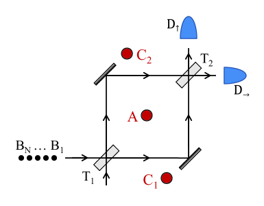
Figure 2.2: An idealized Mach-Zehnder interferometer where the anyons $C$ entangled with the target anyons $A$ are separated into two regions $C_{1}$ and $C_{2}$.

This is a convenient place to note a modest generalization, where the complementary charge $C$ is divided into two regions separated by the interferometer, which we similarly denote as $C_{1}$ and $C_{2}$, respectively. In some experimental setups — e.g. a Fabrey-Pérot interferometer on a quantum Hall bar — each arm of the interferometer individually will separate the region with charge $A$ from a complementary region with respective charges $C_{1}$ and $C_{2}$, which could both be nontrivial. This situation is depicted for the idealized Mach-Zehnder interferometer in Fig. 2.2. In this circumstance, all charge lines from $A$ to $C_{1}$ and from $A$ to $C_{2}$ are (separately) decohered if they can be detected by the probes $B$.

$a$ at 210 650 $c$ at 465 650 $\alpha_{2}$ at 330 570 $\alpha_{1}$ at 350 440 $\alpha_{4}$ at 0 440 $\alpha_{3}$ at 330 50 $e$ at 420 340 $a^{\prime}$ at 210 -40 $c^{\prime}$ at 465 -40 (a) at 280 -130 $c_{1}$ at 990 650 $a$ at 1340 650 $c_{2}$ at 1700 650 $\alpha_{4}$ at 1090 440 $\alpha_{3}$ at 1190 490 $\alpha_{2}$ at 1480 490 $\alpha_{1}$ at 1590 440 $e_{2}$ at 1180 280 $e_{1}$ at 1500 280 $c_{1}^{\prime}$ at 990 -40 $a^{\prime}$ at 1340 -40 $c_{2}^{\prime}$ at 1700 -40 (b) at 1340 -130

Figure 2.3: (a) For a single region of complementary anyons $C$, we show the four positions for the probe loops corresponding to the four terms of Eq. (2.8). (b) For two regions of complementary charge $C_{1}$ and $C_{2}$, the four positions of probe loops are shown on the more complicated the target system (with complementary anyons) density matrix components. (The $4$-valent vertex is understood to be resolved into appropriate trivalent vertices.) $\alpha_{j}$ denotes the weight with which the corresponding probe loop configuration enters the measurement superoperator.