Fractional Poisson Fields and Martingales

Abstract

We present new properties for the Fractional Poisson process and the Fractional Poisson field on the plane. A martingale characterization for Fractional Poisson processes is given. We extend this result to Fractional Poisson fields, obtaining some other characterizations. The fractional differential equations are studied. We consider a more general Mixed-Fractional Poisson process and show that this process is the stochastic solution of a system of fractional differential-difference equations. Finally, we give some simulations of the Fractional Poisson field on the plane.

journalname

t2N. Leonenko was supported in particular by Cardiff Incoming Visiting Fellowship Scheme and International Collaboration Seedcorn Fund and Australian Research Council’s Discovery Projects funding scheme (project number DP160101366)

There are several different approaches to the fundamental concept of Fractional Poisson process (FPP) on the real line. The “renewal” definition extends the characterization of the Poisson process as a sum of independent non-negative exponential random variables. If one changes the law of interarrival times to the Mittag-Leffler distribution (see [32, 33, 44]), the FPP arises. A second approach is given in [6], where the renewal approach to the Fractional Poisson process is developed and it is proved that its one-dimensional distributions coincide with the solution to fractionalized state probabilities. In [34] it is shown that a kind of Fractional Poisson process can be constructed by using an “inverse subordinator”, which leads to a further approach.

In [26], following this last method, the FPP is generalized and defined afresh, obtaining a Fractional Poisson random field (FPRF) parametrized by points of the Euclidean space $\mathbb{R}_{+}^{2}$, in the same spirit it has been done before for Fractional Brownian fields, see, e.g., [17, 20, 22, 30].

The starting point of our extension will be the set-indexed Poisson process which is a well-known concept, see, e.g., [17, 22, 37, 38, 47].

In this paper, we first present a martingale characterization of the Fractional Poisson process. We extend this characterization to FPRF using the concept of increasing path and strong martingales. This characterization permits us to give a definition of a set-indexed Fractional Poisson process. We study the fractional differential equation for FPRF. Finally, we study Mixed-Fractional Poisson processes.

The paper is organized as follows. In the next section, we collect some known results from the theory of subordinators and inverse subordinators, see [8, 36, 49, 50] among others. In Section 2, we prove a martingale characterization of the FPP, which is a generalization of the Watanabe Theorem. In Section 3, another generalization called “Mixed-Fractional Poisson process” is introduced and some distributional properties are studied as well as Watanabe characterization is given. Section 4 is devoted to FPRF. We begin by computing covariance for this process, then we give some characterizations using increasing paths and intensities. We present a Gergely-Yeshow characterization and discuss random time changes. Fractional differential equations are discussed on Section 5.

Finally, we present some simulations for the FPRF.

1 Inverse Subordinators

This section collects some known resuts from the theory of subordinators and inverse subordinators [8, 36, 49, 50].

1.1 Subordinators and their inverse

Consider an increasing Lévy process $L=\{L(t),\ t\geq 0\},$ starting from $0,$ which is continuous from the right with left limits (cadlag), continuous in probability, with independent and stationary increments. Such a process is known as a Lévy subordinator with Laplace exponent

$$\phi(s)=\mu s+\int_{(0,\infty)}(1-e^{-sx})\Pi(dx),\quad s\geq 0,$$

where $\mu\geq 0$ is the drift and the Lévy measure $\Pi$ on $\mathbb{R}_{+}\cup\left\{0\right\}$ satisfies

$$\int_{0}^{\infty}\min(1,x)\Pi(dx)<\infty.$$

This means that

$$\mathrm{E}e^{-sL(t)}=e^{-t\phi(s)},\ s\geq 0.$$

Consider the inverse subordinator $Y(t),\ t\geq 0,$ which is given by the first-passage time of $L:$

$$Y(t)=\inf\left\{u\geq 0:L(u)>t\right\},t\geq 0.$$

The process $Y(t),\ t\geq 0,$ is non-decreasing and its sample paths are a.s. continuous if $L$ is strictly increasing.

We have

$$\left\{(u_{i},t_{i})\colon L(u_{i})<t_{i},i=1,\ldots,n\right\}=\left\{(u_{i},t_{i})\colon Y(t_{i})>u_{i},i=1,\ldots,n\right\},$$

and it is known [39, 41, 49, 50] that for any $p>0,\mathrm{E}Y^{p}(t)<\infty$.

Let $U(t)=\mathrm{E}Y(t)$ be the renewal function. Since

$$\tilde{U}(s)=\int_{0}^{\infty}U(t)e^{-st}dt=\frac{1}{s\phi(s)},$$

then $\tilde{U}$ characterizes the inverse process $Y$, since $\phi$ characterizes $L.$

We get a covariance formula [49, 50]

$$\mathrm{Cov}(Y(t),Y(s))=\int_{0}^{\min(t,s)}\mspace{-50.0mu}(U(t-\tau)+U(s-\tau))dU(\tau)-U(t)U(s).$$

The most important example is considered in the next section, but there are some other examples.

1.2 Inverse stable subordinators

Let $L_{\alpha}=\{L_{\alpha}(t),t\geq 0\}$, be an $\alpha-$stable subordinator with $\phi(s)=s^{\alpha},0<\alpha<1$. The density of $L_{\alpha}(1)$ is of the form [48]

$$g_{\alpha}(x)=\frac{1}{\pi}\mathop{\displaystyle\sum}\limits_{k=1}^{\infty}(-1)^{k+1}\frac{\Gamma(\alpha k+1)}{k!}\frac{1}{x^{\alpha k+1}}\sin(\pi k\alpha)=\frac{1}{x}W_{-\alpha,0}(-x^{-\alpha}).$$ (1.1)

Here we use the Wright’ s generalized Bessel function (see, e.g., [16])

$$W_{\gamma,\beta}(z)=\mathop{\displaystyle\sum}\limits_{k=0}^{\infty}\frac{z^{k}}{\Gamma(1+k)\Gamma(\beta+\gamma k)},\quad z\in\mathbb{C},$$ (1.2)

where $\gamma>-1,$ and $\beta\in\mathbb{R}$. The set of jump times of $L_{\alpha}$ is a.s. dense. The Lévy subordinator is strictly increasing, since the process $L_{\alpha}$ admits a density.

Then the inverse stable subordinator

$$Y_{\alpha}(t)=\inf\{u\geq 0:L_{\alpha}(u)>t\}$$

has density [36, p.110] (see also [43])

$$f_{\alpha}(t,x)=\frac{d}{dx}\mathrm{P}\{Y_{\alpha}(t)\leq x\}=\frac{t}{\alpha}x^{-1-\frac{1}{\alpha}}g_{\alpha}(tx^{-\frac{1}{\alpha}}),\quad x>0,\quad t>0.$$ (1.3)

The Laplace transform of the density $f_{a}(t,x)$ is

$$\int_{0}^{\infty}e^{-st}f_{\alpha}(t,x)dt=s^{\alpha-1}e^{-xs^{\alpha}},\quad s\geq 0,$$ (1.4)

Its paths are continuous and nondecreasing. For $\alpha=1/2,$ the inverse stable subordinator is the running supremum process of Brownian motion, and for $\alpha\in(0,1/2)$ this process is the local time at zero of a strictly stable Lévy process of index $\alpha/(1-\alpha).$

Let

$$E_{\alpha}(z)=\sum_{k=0}^{\infty}\frac{z^{k}}{\Gamma(\alpha k+1)},\ \alpha>0,\ z\in\mathbb{C}$$ (1.5)

be the Mittag-Leffler function [16], and recall the following:

i) The Laplace transform of function $E_{\alpha}(-\lambda t^{\alpha})$ is of the form

$$\int_{0}^{\infty}e^{-st}E_{\alpha}(-\lambda t^{\alpha})dt=\frac{s^{\alpha-1}}{\lambda+s^{\alpha}},\quad 0<\alpha<1,\ t\geq 0,\Re(s)>|\lambda|^{1/\alpha}.$$

(ii) The function $E_{\alpha}(\lambda t^{\alpha})$ is an eigenfunction at the the fractional Caputo-Djrbashian derivative $\mathrm{D}_{t}^{\alpha}$ with eigenvalue $\lambda$ [36, p.36]

$$\mathrm{D}_{t}^{\alpha}E_{\alpha}(\lambda t^{\alpha})=\lambda E_{\alpha}(\lambda t^{\alpha}),\quad 0<\alpha<1,\lambda\in\mathbb{R},$$

where $\mathrm{D}_{t}^{\alpha}$ is defined as (see [36])

$$\mathrm{D}_{t}^{\alpha}u(t)=\frac{1}{\Gamma(1-\alpha)}\int_{0}^{t}\frac{du(\tau)}{d\tau}\frac{d\tau}{(t-\tau)^{\alpha}},\quad 0<\alpha<1.$$ (1.6)

Note that the classes of functions for which the Caputo-Djrbashian derivative is well defined are discussed in [36, Sections 2.2. and 2.3] (in particular one can use the class of absolutely continuous functions).

Proposition 1.1.

The $\alpha$-stable inverse subordinators satisfy the following properties:

1. $$\mathrm{E}e^{-sY_{\alpha}(t)}=\sum_{n=0}^{\infty}\frac{(-st^{\alpha})^{n}}{\Gamma(\alpha n+1)}=E_{\alpha}(-st^{\alpha}),\quad s>0.$$

2. Both processes $L_{\alpha}(t),t\geq 0$ and $Y_{\alpha}(t)$ are self-similar

   $$\frac{L_{\alpha}(at)}{a^{1/\alpha}}\overset{d}{=}L_{\alpha}(t),\;\frac{Y_{\alpha}(at)}{a^{\alpha}}\overset{d}{=}Y_{\alpha}(t),\quad a>0.$$

3. For $0<t_{1}<\cdots<t_{k}$,

   $$\frac{\partial^{k}\mathrm{E}(Y_{\alpha}(t_{1})\cdots Y_{\alpha}(t_{k}))}{\partial t_{1}\cdots\partial t_{k}}=\frac{1}{\Gamma^{k}(\alpha)}\frac{1}{\left[t_{1}(t_{2}-t_{1})\cdots(t_{k}-t_{k-1})\right]^{1-\alpha}}.$$

   In particular,

   (A)

   $$\mathrm{E}Y_{\alpha}(t)=\frac{t^{\alpha}}{\Gamma(1+\alpha)};\mathrm{E[}Y_{\alpha}(t)]^{\nu}=\frac{\Gamma(\nu+1)}{\Gamma(\alpha\nu+1)}t^{\alpha\nu},\quad\nu>0;$$

   (B)

   $$\mathrm{Cov}(Y_{\alpha}(t),Y_{\alpha}(s))=\frac{1}{\Gamma(1+\alpha)\Gamma(\alpha)}\int_{0}^{\min(t,s)}\left((t-\tau)^{\alpha}+(s-\tau)^{\alpha}\right)\tau^{\alpha-1}d\tau-\frac{(st)^{\alpha}}{\Gamma^{2}(1+\alpha)}.$$ (1.7)

Proof.

See [8, 49, 50]. ∎

1.3 Mixture of inverse subordinators

This subsection collects some results from the theory of inverse subordinators, see [49, 50, 36, 5, 28].

Different kinds of inverse subordinators can be considered.

Let $L_{\alpha_{1}}$ and $L_{\alpha_{2}}$ be two independent stable subordinators. The mixture of them $L_{\alpha_{1},\alpha_{2}}=\{L_{\alpha_{1},\alpha_{2}}(t),t\geq 0\}$ is defined by its Laplace transform: for $s\geq 0,\ C_{1}+C_{2}=1,\ C_{1}\geq 0,\ C_{2}\geq 0,\ \alpha_{1}<\alpha_{2}$,

$$\mathrm{E}e^{-sL_{\alpha_{1},\alpha_{2}}(t)}=\exp\{-t(C_{1}s^{\alpha_{1}}+C_{2}s^{\alpha_{2}})\}.$$ (1.8)

It is possible to prove that

$$L_{\alpha_{1},\alpha_{2}}(t)=(C_{1})^{\frac{1}{\alpha_{1}}}L_{\alpha_{1}}(t)+(C_{2})^{\frac{1}{\alpha_{2}}}L_{\alpha_{2}}(t),\quad t\geq 0,$$

is not self-similar, unless $\alpha_{1}=\alpha_{2}=\alpha,$ since $L_{\alpha_{1},\alpha_{2}}(at)=^{d}(C_{1})^{\frac{1}{\alpha_{1}}}a^{\frac{1}{\alpha_{1}}}L_{\alpha_{1}}(t)+(C_{2})^{\frac{1}{\alpha_{2}}}a^{\frac{1}{\alpha_{2}}}L_{\alpha_{2}}(t).$ This expression is equal to $a^{\frac{1}{\alpha}}L_{\alpha_{1},\alpha_{2}}(t)$ for any $t>0$ if and only if $\alpha_{1}=\alpha_{2}=\alpha,$ in which case the process $L_{\alpha_{1},\alpha_{2}}$ can be reduced to the classical stable subordinator (up to a constant).

The inverse subordinator is defined by

$$Y_{\alpha_{1},\alpha_{2}}(t)=\inf\{u\geq 0:L_{\alpha_{1},\alpha_{2}}(u)>t\},\quad t\geq 0.$$ (1.9)

We assume that $C_{2}\neq 0$ without loss of generality (the case $C_{2}=0$ reduces to the previous case of single inverse subordinator).

It was proved in [28] that

$$\tilde{U}(t)=\frac{1}{(C_{1}s^{\alpha_{1}}+C_{2}s^{\alpha_{2}})s},U(t)=\frac{1}{C_{2}}t^{\alpha_{2}}E_{\alpha_{2}-\alpha_{1},\alpha_{2}+1}(-\tfrac{C_{1}}{C_{2}}t^{{}_{\alpha_{2}-\alpha_{1}}}),$$ (1.10)

where $E_{\alpha,\beta}(z)$ is the two-parametric Generalized Mittag-Leffler function ([14, 16])

$$E_{\alpha,\beta}(z)=\sum_{k=0}^{\infty}\frac{z^{k}}{\Gamma(\alpha k+\beta)},\ \alpha>0,\beta>0,\ z\in\mathbb{C}.$$

Also for the Laplace transform of the density $f_{\alpha_{1},\alpha_{2}}(t,u)=\frac{d}{du}\mathrm{P}\{Y_{\alpha_{1},\alpha_{2}}(t)\leq u\},$ $u\geq 0,$ of the inverse subordinator $Y_{\alpha_{1},\alpha_{2}}=\{Y_{\alpha_{1},\alpha_{2}}(t),t\geq 0\},$ we have the following expression [35]:

$$\tilde{f}_{\alpha_{1},\alpha_{2}}(s,u)=\int_{0}^{\infty}e^{-st}f_{\alpha_{1},\alpha_{2}}(t,u)dt=\frac{1}{s}[C_{1}s^{\alpha_{1}}+C_{2}s^{\alpha_{2}}]e^{-u[C_{1}s^{\alpha_{1}}+C_{2}s^{\alpha_{2}}]},\quad s\geq 0,$$ (1.11)

and the Laplace transform of $\tilde{f}$ is given by

$$\int_{0}^{\infty}e^{-pu}\tilde{f}_{\alpha_{1},\alpha_{2}}(s,u)du=\frac{\phi(s)}{s(p+\phi(s))}=\frac{C_{1}s^{\alpha_{1}-1}+C_{2}s^{\alpha_{2}-1}}{p+C_{1}s^{\alpha_{1}}+C_{2}s^{\alpha_{2}}},\quad p\geq 0.$$ (1.12)

From [5, Theorem 2.3] we have the following expression for $u\geq 0,t>0$:

$$f_{\alpha_{1},\alpha_{2}}(t,u)=\frac{C_{1}}{\lambda t^{\alpha_{1}}}\sum_{r=0}^{\infty}\frac{1}{r!}(-\frac{C_{2}\left|u\right|}{\lambda t^{\alpha_{2}}})^{r}W_{-\alpha_{1},1-\alpha_{2}r-\alpha_{1}}(-\frac{C_{1}\left|u\right|}{\lambda t^{\alpha_{1}}})+$$

$$+\frac{C_{2}}{\lambda t^{\alpha_{2}}}\sum_{r=0}^{\infty}\frac{1}{r!}(-\frac{C_{1}\left|u\right|}{\lambda t^{\alpha_{1}}})^{r}W_{-\alpha_{2},1-\alpha_{1}r-\alpha_{2}}(-\frac{C_{2}\left|u\right|}{\lambda t^{\alpha_{2}}}).$$ (1.13)

One can also consider the tempered stable inverse subordinator, the inverse subordinator to the Poisson process, the compound Poisson process with positive jumps, the Gamma and the inverse Gaussian Lévy processes. For additional details see [28, 49, 50].

2 Fractional Poisson Processes and Martingales

2.1 Preliminaries

The first definition of FPP $N_{\alpha}=\{N_{\alpha}(t),t\geq 0\}$ was given in [32] (see also [33]) as a renewal process with Mittag-Leffler waiting times between the events

$$N_{\alpha}(t)=\max\left\{n:T_{1}+...+T_{n}\leq t\right\}=\sum_{j=1}^{\infty}{\mathbbm{1}}_{\{T_{1}+...+T_{j}\leq t\}},\qquad t\geq 0,$$

where $\left\{T_{j}\right\},$ $j=1,2,\ldots$ are iid random variables with the strictly monotone Mittag-Leffler distribution function

$$F_{\alpha}(t)=\mathrm{P}\left(T_{j}\leq t\right)=1-E_{\alpha}(-\lambda t^{\alpha}),\qquad t\geq 0,0<\alpha<1,\quad j=1,2,\ldots$$

The following stochastic representation for FPP is found in [34]:

$$N_{\alpha}(t)=N(Y_{\alpha}(t)),\quad t\geq 0,\quad\alpha\in(0,1),$$

where $N=\{N(t),t\geq 0\},$ is the classical homogeneous Poisson process with parameter $\lambda>0,$ which is independent of the inverse stable subordinator $Y_{\alpha}.$ One can compute the following expression for the one-dimensional distribution of FPP (see [46]):

$$\mathrm{P}\left(N_{\alpha}(t)=k\right) =p_{k}^{(\alpha)}(t)=\int_{0}^{\infty}\frac{e^{-\lambda x}(\lambda x)^{k}}{k!}f_{\alpha}(t,x)dx$$

$$=\frac{(\lambda t^{\alpha})^{k}}{k!}\mathop{\displaystyle\sum}\limits_{j=1}^{\infty}\frac{(k+j)!}{j!}\frac{(-\lambda t^{\alpha})^{j}}{\Gamma(\alpha(j+k)+1)}=\frac{\left(\lambda t^{\alpha}\right)^{k}}{k!}E_{\alpha}^{(k)}(-\lambda t^{\alpha})$$

$$=(\lambda t^{\alpha})^{k}E_{\alpha,\alpha k+1}^{k+1}(-\lambda t^{\alpha}),\quad k=0,1,2...,t\geq 0,\quad 0<\alpha<1,$$

where $f_{\alpha}$ is given by (1.3), $E_{\alpha}(z)$ is the Mittag-Leffler function (1.5), $E_{\alpha}^{(k)}(z)$ is the $k-$th derivative of $E_{\alpha}(z)$, and $E_{\alpha,\beta}^{\gamma}(z)$ is the three-parametric Generalized Mittag-Leffler function defined as follows [16, 42]:

$$E_{\alpha,\beta}^{\gamma}(z)=\sum_{j=0}^{\infty}\frac{(\gamma)_{j}z^{j}}{j!\Gamma(\alpha j+\beta)},\alpha>0,\beta>0,\ \gamma>0,\quad z\in\mathbb{C},$$ (2.1)

where

$$(\gamma)_{j}=\begin{cases}1&\text{if }j=0;\\ \gamma(\gamma+1)\cdots(\gamma+j-1)&\text{if }j=1,2,\ldots\end{cases}$$

is the Pochhammer symbol.

Finally, in [6, 7] it is shown that the marginal distribution of FPP satisfies the following system of fractional differential-difference equations (see [25]):

$$\mathrm{D}_{t}^{\alpha}p_{k}^{(\alpha)}(t)=-\lambda(p_{k}^{(\alpha)}(t)-p_{k-1}^{(\alpha)}(t)),\quad k=0,1,2,\ldots$$

with initial conditions: $p_{0}^{(\alpha)}(0)=1,p_{k}^{(\alpha)}(0)=0,k\geq 1,$ and $p_{-1}^{(\alpha)}(t)=0,$ where $\mathrm{D}_{t}^{\alpha}$ is the fractional Caputo-Djrbashian derivative (1.6). See also [11].

Remark.

Note that

$$\mathrm{E}N_{\alpha}(t)=\mathrm{E}\big{[}\mathrm{E}[N(Y_{\alpha}(t))|Y_{\alpha}(t)]\big{]}=\int_{0}^{\infty}[\mathrm{E}N(u)]f_{\alpha}(t,u)du=\lambda t^{\alpha}/\Gamma(1+\alpha),$$

where $f_{\alpha}(t,u)$ is given by (1.3), and [28] showed that

$$\mathrm{Cov}(N_{\alpha}(t),N_{\alpha}(s))=\frac{\lambda(\min(t,s))^{\alpha}}{\Gamma(1+\alpha)}+\lambda^{2}\mathrm{Cov}(Y_{\alpha}(t),Y_{\alpha}(s)),$$ (2.2)

where $\mathrm{Cov}(Y_{\alpha}(t),Y_{\alpha}(s))$ is given in (1.7) while $\mathrm{Cov}(N(t),N(s))=\lambda\min(t,s)$. In particular,

$$\mathrm{Var}N_{\alpha}(t) =\lambda^{2}t^{2\alpha}\Big{[}\frac{2}{\Gamma(1+2\alpha)}-\frac{1}{\Gamma^{2}(1+\alpha)}\Big{]}+\frac{\lambda t^{\alpha}}{\Gamma(1+\alpha)}$$ (2.3)

$$=\frac{\lambda^{2}t^{2\alpha}}{\Gamma^{2}(1+\alpha)}\Big{(}\frac{\alpha\Gamma(\alpha)}{\Gamma(2\alpha)}-1\Big{)}+\frac{\lambda t^{\alpha}}{\Gamma(1+\alpha)},\quad t\geq 0.$$

The definition of the Hurst index for renewal processes is discussed in [14]. In the same spirit, one can define the analogous of the Hurst index for the FPP as

$$H=\inf\left\{\beta:\lim\sup_{T\rightarrow\infty}\frac{\mathrm{Var}N_{\alpha}(T)}{{T^{2\beta}}}<\infty\right\}\in(0,1).$$

To prove the formula (2.2), one can use the conditional covariance formula [45, Exercise 7.20.b]:

$$\mathrm{Cov}(Z_{1},Z_{2})=\mathrm{E}\big{(}\mathrm{Cov}(Z_{1},Z_{2}|Y)\big{)}+\mathrm{Cov}\big{(}\mathrm{E}(Z_{1}|Y),\mathrm{E}(Z_{2}|Y)\big{)},$$

where $Z_{1},Z_{2}$ and $Y$ are random variables, and

$$\mathrm{Cov}(Z_{1},Z_{2}|Y)=\mathrm{E}\big{(}(Z_{1}-\mathrm{E}(Z_{1}|Y))(Z_{2}-\mathrm{E}(Z_{2}|Y))\big{)}.$$

Really, if

$$G_{t,s}(u,v)=\mathrm{P}\{Y_{\alpha}(t)\leq u,Y_{\alpha}(s)\leq v\},$$

then $\mathrm{E}(N(Y_{\alpha}(t))|Y_{\alpha}(t))=\mathrm{E}(N(1))\cdot Y_{\alpha}(t)=\lambda Y_{\alpha}(t)$, and

$$\mathrm{Cov}(Y_{\alpha}(t),Y_{\alpha}(s))=\mathrm{Var}\Big{(}N(1)\int_{0}^{\infty}\int_{0}^{\infty}\min(u,v)G_{t,s}(du,dv)\Big{)}+\mathrm{Cov}\big{(}\lambda Y_{\alpha}(t),\lambda Y_{\alpha}(s)\big{)}\\ =\lambda\mathrm{E}(Y_{\alpha}(\min(t,s)))+\lambda^{2}\mathrm{Cov}(Y_{\alpha}(t),Y_{\alpha}(s)),$$

since, for example, if $s\leq t$, then $v=Y_{\alpha}(s)\leq Y_{\alpha}(t)=u$, and

$$\int_{0}^{\infty}\int_{0}^{\infty}vG_{t,s}(du,dv)=\int_{0}^{\infty}v\int_{0}^{\infty}G_{t,s}(du,dv)=\int_{0}^{\infty}v\,d\mathrm{P}\{Y_{\alpha}(s)\leq v\}=\mathrm{E}(Y_{\alpha}(s)).$$

Remark.

For more than one random variable in the condition, the conditional covariance formula becomes more complicated, it can be seen even for the conditional variance formula:

$$\mathrm{Var}(Z)=\mathrm{E}\big{(}\mathrm{Var}(Z|Y_{1},Y_{2})\big{)}+\mathrm{E}\big{(}\mathrm{Var}[\mathrm{E}(Z|Y_{1},Y_{2})]|Y_{1}\big{)}+\mathrm{Var}\big{(}\mathrm{E}(Z|Y_{1})\big{)}.$$

The corresponding formulas can be found in [9]. That is why for random fields we develop another technique, see Appendix.

2.2 Watanabe characterization

Let $\left(\Omega,\mathcal{F},\mathrm{P}\right)$ be a complete probability space. Recall that the $\mathcal{F}_{t}-$adapted, $\mathrm{P}$-integrable stochastic process $M=\{M(t),t\geq 0\}$ is an $\mathcal{F}_{t}-$martingale (sub-martingale) if $\mathrm{E}(M(t)|\mathcal{F}_{s})=(\geq)M(s),$ $0\leq s\leq t,$ a.s., where $\{\mathcal{F}_{t}\}$ is a non-decreasing family of sub-sigma fields of $\mathcal{F}$. A point process $N$ is called simple if its jumps are of magnitude $+1$. It is locally finite when it does not have infinite jumps in a bounded region. The following theorem is known as the Watanabe characterization for homogeneous Poisson processes (see, [51] and [10, p. 25]):

Theorem 2.1.

Let $N=\{N(t),t\geq 0\}$ be a $\mathcal{F}_{t}-$adapted, simple locally finite point process. Then $N$ is a homogeneous Poisson process iff there is a constant $\lambda>0$, such that the process $M(t)=N(t)-\lambda t$ is an $\mathcal{F}_{t}-$martingale.

We extend the well-known Watanabe characterization for FPP. The following result may be seen as a corollary of the Watanabe characterization for Cox processes as in [10, Chapetr II]. We will make use of the following lemma.

Lemma 2.1 (Doob’s Optional Sampling Theorem).

Let $M$ be a right-continuous martingale. Then, if $T$ and $S$ are stopping times such that $P(T<+\infty)=1$ and $\{M(t\wedge T),t\geq 0\}$ is uniformly integrable, then $E(M(T)|\mathcal{F}_{S\wedge T})=M(S\wedge T)$.

Proof.

Define $N=\{N(t)=M(t\wedge T),t\geq 0\}$. Then $N$ is a right-continuous uniformly integrable martingale such that $\lim_{t\to+\infty}N(t)=M(T)$. Moreover, $N(S)=M(T\wedge S)$. The thesis is hence a consequence of the Doob’s Optional Sampling Theorem (see, e.g., [23, Theorem 7.29] with $X=N$, $\tau\equiv+\infty$ and $\sigma=S$). ∎

Theorem 2.2.

Let $X=\{X(t),\,t\geq 0\}$ be a simple locally finite point process. Then $X$ is a FPP iff there exist a constant $\lambda>0,$ and an $\alpha$-stable subordinator $L_{\alpha}=\{L_{\alpha}(t),\,t\geq 0\},$ $0<\alpha<1,$ such that, denoted by $Y_{\alpha}(t)=\inf\{s:L_{\alpha}(s)\geq t\}$ its inverse stable subordinator, the process

$$M=\{M(t),\,t\geq 0\}=\{X(t)-\lambda Y_{\alpha}(t),\,t\geq 0\}$$

is a right-continuous martingale with respect to the induced filtration $\mathcal{F}_{t}=\sigma(X(s),s\leq t)\vee\sigma(Y_{\alpha}(s),s\geq 0)$ such that, for any $T>0$,

$$\{M(\tau),\tau\text{ stopping time s.t.\ }Y_{\alpha}(\tau)\leq T\}$$ (2.4)

is uniformly integrable.

Proof.

If $X$ is a FPP, then $X(t)=N(Y_{\alpha}(t)),$ where $Y_{\alpha}$ is the inverse of an $\alpha$-stable subordinator and $N$ is a Poisson process with intensity $\lambda>0.$

Note that $X\geq 0$ and $(Y_{\alpha}\geq 0$ are monotone non-decreasing, and hence the boundenesses in $L^{2}$ given by (2.3) and Proposition 1.1 iiiA) imply that $\{N(Y_{\alpha}(t))-\lambda Y_{\alpha}(t),0\leq t\leq T\}$ is uniformly integrable (see, for example, [23, pag. 67]). Therefore $N(Y_{\alpha}(t))-\lambda Y_{\alpha}(t)$ is still a martingale, by Lemma 2.1. Notice that $Y_{\alpha}(t)$ is continuous increasing and adapted; therefore it is the predictable intensity of the sub-martingale $X.$

Now, let $\tau$ be a stopping time s.t. $Y_{\alpha}(\tau)\leq T$, and hence $\lambda Y_{\alpha}(\tau)\leq\lambda T$. Then, since $N$ is a Poisson process with intensity $\lambda>0$, $\tilde{M}(t)=M(\tau\wedge t)$ is a martingale bounded in $L^{2}$ and null at $0$, and therefore it converges in $L^{2}$ to $M(\tau)$, with variance bounded by

$$E(M^{2}(\tau))=\lim_{t\to\infty}E(M^{2}(\tau\wedge t))\leq\mathrm{Var}(N(T))+\mathrm{Var}(Y_{\alpha}(\tau))\leq\text{const}\cdot(1+T^{2}).$$

Then the family (2.4) is uniformly bounded in $L^{2}$, which implies the thesis.

Conversely, it is enough to prove that $X(t)=N(Y_{\alpha}(t)),$ where $N$ is a Poisson process, independent of $Y_{\alpha}.$

Consider the inverse of $Y_{\alpha}(t):$

$$Z(t)=\inf\{s:\,Y_{\alpha}(s)\geq t\}.$$

$\{Z(t),\,t\geq 0\}$ can be seen as a family of stopping times. Then, by Lemma 2.1,

$$M(Z(t))=X(Z(t))-\lambda Y_{\alpha}(Z(t))$$

is still a martingale. The fact that $Y_{\alpha}$ is continuous implies that $Y_{\alpha}(Z(t))=t$, and hence $X(Z(t))-\lambda t$ is a martingale. Moreover, since $Z(t)$ is increasing, $X(Z(t))$ is a simple point process.

Following the classical Watanabe characterization, $X(Z(t))$ is a classical Poisson process with parameter $\lambda>0$. Call this process $N(t)=X(Z(t)).$ Then $X(t)=N(Y_{\alpha}(t))$ is a FPP. ∎

For recent developments and random change time results, see also [31, 40]. In particular, we thank a referee to have outlined that a similar result has been obtained in [40, Lemma 3.2].

3 Mixed-Fractional Poisson Processes

3.1 Definition

In this section, we consider a more general Mixed-Fractional Poisson process (MFPP)

$$N^{\alpha_{1},\alpha_{2}}=\{N^{\alpha_{1},\alpha_{2}}(t),t\geq 0\}=\{N(Y_{\alpha_{1},\alpha_{2}}(t)),t\geq 0\},$$ (3.1)

where the homogeneous Poisson process $\ N$ with intensity $\lambda>0,$ and the inverse subordinator $Y_{\alpha_{1},\alpha_{2}}$ given by (1.9) are independent. We will show that $N^{\alpha_{1},\alpha_{2}}$ is the stochastic solution of the system of fractional differential-difference equations: for $k=0,1,2,\ldots$,

$$C_{1}\mathrm{D}_{t}^{\alpha_{1}}p_{k}^{(\alpha_{1},\alpha_{2})}(t)+C_{2}\mathrm{D}_{t}^{\alpha_{2}}p_{k}^{(\alpha_{1},\alpha_{2})}(t)=-\lambda(p_{k}^{(\alpha_{1},\alpha_{2})}(t)-p_{k-1}^{(\alpha_{1},\alpha_{2})}(t)),$$ (3.2)

with initial conditions:

$$p_{0}^{(\alpha_{1},\alpha_{2})}(0)=1,p_{k}^{(\alpha_{1},\alpha_{2})}(0)=0,p_{-1}^{(\alpha_{1},\alpha_{2})}(t)=0,\quad k\geq 1,$$ (3.3)

where $\mathrm{D}_{t}^{\alpha}$ is the fractional Caputo-Djrbashian derivative (1.6), and for $C_{1}\geq 0,C_{2}>0,C_{1}+C_{2}=1$, $\alpha_{1},\alpha_{2}\in(0,1)$,

$$p_{k}^{(\alpha_{1},\alpha_{2})}(t)=\mathrm{P}\{N^{\alpha_{1},\alpha_{2}}(t)=k\},\qquad k=0,1,2\ldots$$

3.2 Distribution Properties

Using the formulae for Laplace transform of the fractional Caputo-Djrbashian derivative (see, [36, p.39]):

$$\int_{0}^{\infty}e^{-st}\mathrm{D}_{t}^{\alpha}u(t)dt=s^{\alpha}u(0^{+})-s^{\alpha-1}u(0),0<\alpha<1,$$

one can obtain from (3.2) with $k=0$ the following equation

$$C_{1}s^{\alpha_{1}}\tilde{p}_{0}(s)-C_{1}s^{\alpha_{1}-1}+C_{2}s^{\alpha 2}\tilde{p}_{0}(s)-C_{2}s^{\alpha_{2}-1}=-\lambda\tilde{p}_{0}(s),\tilde{p}_{0}(0)=1,$$

for the Laplace transform

$$\tilde{p}_{0}^{(\alpha_{1},\alpha_{2})}(s)=\tilde{p}_{0}(s)=\int_{0}^{\infty}e^{-st}p_{0}^{(\alpha_{1},\alpha_{2})}(t)dt,\quad s\geq 0.$$

Thus

$$\tilde{p}_{0}(s)=\frac{C_{1}s^{\alpha_{1}-1}+C_{2}s^{\alpha_{2}-1}}{\lambda+C_{1}s^{\alpha_{1}}+C_{2}s^{\alpha_{2}}},\quad s\geq 0,$$

and using the formula for an inverse Laplace transform (see, [16]), for $\Re\alpha>0,\Re\beta>0,\Re s>0,\Re(\alpha-\rho)>0,\Re(\alpha-\beta)>0,$ and $|as^{\beta}/(s^{\alpha}+b)|<1$:

$$\mathcal{L}^{-1}\Big{(}\frac{s^{\rho-1}}{s^{\alpha}+as^{\beta}+b};t\Big{)}=t^{\alpha-\rho}\sum_{r=0}^{\infty}(-a)^{r}t^{(\alpha-\beta)r}E_{\alpha,\alpha+(\alpha-\beta)r-\rho+1}^{r+1}(-bt^{\alpha}),$$ (3.4)

one can find an exact form of the $p_{0}^{(\alpha_{1},\alpha_{2})}(t)$ in terms of generalized Mittag-Leffler functions (2.1):

$$p_{0}^{(\alpha_{1},\alpha_{2})}(t) =\mathop{\displaystyle\sum}\limits_{r=0}^{\infty}\left(-\frac{C_{1}}{C_{2}}t^{\alpha_{2}-\alpha_{1}}\right)^{r}E_{\alpha_{2},(\alpha_{2}-\alpha_{1})r+1}^{r+1}\left(-\frac{\lambda}{C_{2}}t^{\alpha_{2}}\right)$$ (3.5)

$$\quad-\mathop{\displaystyle\sum}\limits_{r=0}^{\infty}\left(-\frac{C_{1}}{C_{2}}t^{\alpha_{2}-\alpha_{1}}\right)^{r+1}E_{\alpha_{2},(\alpha_{2}-\alpha_{1})(r+1)+1}^{r+1}\left(-\frac{\lambda}{C_{2}}t^{\alpha_{2}}\right).$$

For $k\geq 1,$we obtain from (3.2):

$$\tilde{p}_{k}(s)(\lambda+C_{1}s^{\alpha_{1}}+C_{2}s^{\alpha_{2}})=\lambda\tilde{p}_{k-1}(s),$$

where

$$\tilde{p}_{k}^{(\alpha_{1},\alpha_{2})}(s)=\tilde{p}_{k}(s)=\int_{0}^{\infty}e^{-st}p_{k}^{(\alpha_{1},\alpha_{2})}(t)dt,\quad s\geq 0.$$

Thus from (3.2) we obtain the following expression for the Laplace transform of $p_{k}^{(\alpha_{1},\alpha_{2})}(t),$ $k\geq 0:$

$$\tilde{p}_{k}(s) =\left(\frac{\lambda}{\lambda+C_{1}s^{\alpha_{1}}+C_{2}s^{\alpha_{2}}}\right)\tilde{p}_{k-1}(s)=\left(\frac{\lambda}{\lambda+C_{1}s^{\alpha_{1}}+C_{2}s^{\alpha_{2}}}\right)^{k}\tilde{p}_{0}(s)$$ (3.6)

$$=\frac{\lambda^{k}(C_{1}s^{\alpha_{1}-1}+C_{2}s^{\alpha_{2}-1})}{(\lambda+C_{1}s^{\alpha_{1}}+C_{2}s^{\alpha_{2}})^{k+1}}=\frac{\lambda^{k}(C_{1}s^{\alpha_{1}}+C_{2}s^{\alpha_{2}})}{s(\lambda+C_{1}s^{\alpha_{1}}+C_{2}s^{\alpha_{2}})^{k+1}},\ k=0,1,2...$$

On the other hand, one can compute the Laplace transform from the stochastic representation (3.1). If

$$p_{k}^{(\alpha_{1},\alpha_{2})}(t)=\mathrm{P}\{N(Y_{\alpha_{1},\alpha_{2}}(t))=k\}=\int_{0}^{\infty}\frac{e^{-\lambda x}}{k!}(\lambda x)^{k}f_{\alpha_{1},\alpha_{2}}(t,x)dx,$$ (3.7)

where $f_{\alpha_{1},\alpha_{2}}(t,x)$ is given by (1.13), then using (1.11),(1.12) we have for $k\geq 0,s>0$

$$\tilde{p}_{k}(s)=\int_{0}^{\infty}e^{-st}p_{k}^{(\alpha_{1},\alpha_{2})}(t)dt=\int_{0}^{\infty}\frac{e^{-\lambda x}}{k!}(\lambda x)^{k}\Big{[}\int_{0}^{\infty}e^{-st}f_{\alpha_{1},\alpha_{2}}(t,x)dt\Big{]}dx$$

$$=\frac{\lambda^{k}}{k!}\frac{\phi(s)}{s}\int_{0}^{\infty}e^{-\lambda x}x^{k}e^{-x\phi(s)}dx$$

Note that

$$\frac{\partial^{k}}{\partial\lambda^{k}}\int_{0}^{\infty}e^{-\lambda x}e^{-x\phi(s)}dx=(-1)^{k}\int_{0}^{\infty}e^{-\lambda x}x^{k}e^{-x\phi(s)}dx$$

$$\qquad=\frac{\partial^{k}}{\partial\lambda^{k}}\frac{1}{\lambda+\phi(s)}=(-1)^{k}\frac{k!}{(\lambda+\phi(s))^{k+1}};$$

thus

$$\tilde{p}_{k}(s)=\lambda^{k}\frac{\phi(s)}{s(\lambda+\phi(s))^{k+1}}=\frac{\lambda^{k}(C_{1}s^{\alpha_{1}}+C_{2}s^{\alpha_{2}})}{s(\lambda+C_{1}s^{\alpha_{1}}+C_{2}s^{\alpha_{2}})^{k+1}},$$

the same expression as (3.6). We can formulate the result in the following form:

Theorem 3.1.

The MFPP $N^{\alpha_{1},\alpha_{2}}$ defined in (3.1) is the stochastic solution of the system of fractional differential-difference equations (3.2) with initial conditions (3.3).

Note that in [5] one can find some other stochastic representations of the MFPP (3.1). Also, some analytical expression for $p_{0}^{(\alpha_{1},\alpha_{2})}(t)$ is given by (3.5), while the analytical expression for $p_{k}^{(\alpha_{1},\alpha_{2})}(t),$for $k\geq 1,$ are given by (3.7).

Moreover, $p_{k}^{(\alpha_{1},\alpha_{2})}(t),$for $k\geq 1,$ can be obtained by the following recurrent relation:

$$p_{k}^{(\alpha_{1},\alpha_{2})}(t)=\mathop{\displaystyle\int}\limits_{0}^{t}p_{k-1}^{(\alpha_{1},\alpha_{2})}(t-z)g(z)dz,$$

where

$$\tilde{g}(s)=\int_{0}^{\infty}e^{-sz}g(z)dz=\frac{\lambda}{\lambda+C_{1}s^{\alpha_{1}}+C_{2}s^{\alpha_{2}}},$$

and from (3.4):

$$g(z)=\frac{\lambda}{C_{2}}z^{\alpha_{2}-1}\sum_{r=0}^{\infty}\Big{(}-\frac{C_{1}}{C_{2}}z^{\alpha_{2}-\alpha_{1}}\Big{)}^{r}E_{\alpha_{2},\alpha_{2}+(\alpha_{2}-\alpha_{1})r}^{r+1}\Big{(}-\frac{\lambda}{C_{2}}z^{\alpha_{2}}\Big{)}.$$

3.3 Dependence

From [28, Theorem 2.1] and (1.10), we have the following expressions for moments in form of the function

$$U(t) =\frac{1}{C_{2}}t^{\alpha_{2}}E_{\alpha_{2}-\alpha_{1},\alpha_{2}+1}(-C_{1}t^{{}_{\alpha_{2}-\alpha_{1}}}/C_{2}),$$

$$\mathrm{E}N^{\alpha_{1},\alpha_{2}}(t) =\lambda U(t),$$

$$\mathrm{Var}N^{\alpha_{1},\alpha_{2}}(t) =\lambda^{2}\frac{1}{C_{2}^{2}}t^{2\alpha_{2}}[2E_{\alpha_{2}-\alpha_{1},\alpha_{1}+\alpha_{2}+1}(-C_{1}t^{{}_{\alpha_{2}-\alpha_{1}}}/C_{2})$$

$$\qquad-(E_{\alpha_{2}-\alpha_{1},\alpha_{2}+1}(-C_{1}t^{{}_{\alpha_{2}-\alpha_{1}}}/C_{2}))^{2}]$$

$$\qquad+\lambda\frac{1}{C_{2}}t^{\alpha_{2}}E_{\alpha_{2}-\alpha_{1},\alpha_{2}+1}(-C_{1}t^{{}_{\alpha_{2}-\alpha_{1}}}/C_{2}),$$

$$\mathrm{Cov}(N^{\alpha_{1},\alpha_{2}}(t),N^{\alpha_{1},\alpha_{2}}(s)) =\lambda U(\min(t,s))+\lambda^{2}\Big{\{}\int_{0}^{\min(t,s)}\Big{(}U(t-\tau)$$

$$\qquad\qquad+U(s-\tau)\Big{)}dU(\tau)-U(t)U(s)\Big{\}}.$$

We extend the Watanabe characterization for MFPP. Let $\Lambda(t):\mathbb{R}_{+}\to\mathbb{R}_{+}$ be a non-negative right-continuous non-decreasing deterministic function such that $\Lambda(0)=0$, $\Lambda(\infty)=\infty$, and $\Lambda(t)-\Lambda(t-)\leq 1$ for any $t$. Such a function will be called consistent. The Mixed-Fractional Non-homogeneous Poisson process (MFNPP) is defined as

$$N^{\alpha_{1},\alpha_{2}}_{\Lambda}=\{N^{\alpha_{1},\alpha_{2}}_{\Lambda}(t),t\geq 0\}=\{N(\Lambda(Y_{\alpha_{1},\alpha_{2}}(t))),t\geq 0\},$$

where the homogeneous Poisson process $\ N$ with intensity $\lambda=1$, and the inverse subordinator $Y_{\alpha_{1},\alpha_{2}}$ given by (1.9) are independent.

Theorem 3.2.

Let $X=\{X(t),\,t\geq 0\}$ be a simple locally finite point process. $X$ is a MFNPP iff there exist a consistent function $\Lambda(t),$ and a mixed stable subordinator {$L_{\alpha_{1},\alpha_{2}}(t),\,t\geq 0\},$ $0<\alpha_{1}<1,$ $0<\alpha_{2}<1,$ defined in (1.8), such that

$$M=\{M(t),\,t\geq 0\}=\{X(t)-\Lambda(Y_{\alpha_{1},\alpha_{2}}(t)),\,t\geq 0\}$$

is a martingale with respect to the induced filtration $\mathcal{F}_{t}=\sigma(X(s),s\leq t)\vee\sigma(Y_{\alpha_{1},\alpha_{2}}(s),s\geq 0)$, where $Y_{\alpha_{1},\alpha_{2}}(t)=\inf\{s:L_{\alpha_{1},\alpha_{2}}(t)\geq t\}$ is the inverse mixed stable subordinator. In addition, for any $T>0$,

$$\{M(\tau),\tau\text{ stopping time s.t.\ }\Lambda(Y_{\alpha_{1},\alpha_{2}}(\tau))\leq T\}$$

is uniformly integrable.

Proof.

The proof is analogue to that of Theorem 2.2. ∎

4 Two-Parameter Fractional Poisson Processes and Martingales

4.1 Homogeneous Poisson random fields

This section collects some known results from the theory of two-parameter Poisson processes and homogeneous Poisson random fields (PRF) (see, e.g., [47, 37], among the others).

Let $\left(\Omega,\mathcal{F},P\right)$ be a complete probability space and let $\left\{\mathcal{F}_{t_{1},t_{2}};\left(t_{1},t_{2}\right)\in\mathbb{R}_{+}^{2}\right\}$ be a family of sub-$\sigma$-fields of $\mathcal{F}$ such that

(i) $\mathcal{F}_{s_{1},s_{2}}\subseteq\mathcal{F}_{t_{1},t_{2}}$ for any $\quad s_{1}\leq t_{1},\quad s_{2}\leq t_{2};$

(ii) $\mathcal{F}_{0,0}$ contains all null sets of $\mathcal{F};$

(iii) for each $z\in\mathbb{R}_{+}^{2},$ $\mathcal{F}_{z}=\mathop{\displaystyle\bigcap}\limits_{z\prec z^{\prime}}\mathcal{F}_{z^{\prime}}$ where $z=\left(s_{1},s_{2}\right)\prec z^{\prime}=\left(t_{1},t_{2}\right)$ denotes the partial order on $\mathbb{R}_{+}^{2},$ which means that $s_{1}\leq t_{1},\quad s_{2}\leq t_{2}.$

Given $\left(s_{1},s_{2}\right)\prec\left(t_{1},t_{2}\right)$ we denote by

$$\Delta_{s_{1},s_{2}}X(t_{1},t_{2})=X(t_{1},t_{2})-X(t_{1},s_{2})-X(s_{1},t_{2})+X(s_{1},s_{2})$$

the increments of the random field $X(t_{1},t_{2}),(t_{1},t_{2})\in\mathbb{R}_{+}^{2}$ over the rectangle $(\left(s_{1},s_{2}\right),\left(t_{1},t_{2}\right)]$. In addition, we denote

$$\mathcal{F}_{\infty,t_{2}}=\sigma(\mathcal{F}_{t_{1},t_{2}},t_{1}>0),\mathcal{F}_{t_{1},\infty}=\sigma(\mathcal{F}_{t_{1},t_{2}},t_{2}>0),\text{ and }\mathcal{F}^{*}_{s_{1},s_{2}}=\mathcal{F}_{\infty,s_{2}}\vee\mathcal{F}_{s_{1},\infty}=\sigma(\mathcal{F}_{s_{1},\infty},\mathcal{F}_{\infty,s_{2}}).$$

A strong martingale is an integrable two-parameter process $X$ such that

$$E(\Delta_{s_{1},s_{2}}X(t_{1},t_{2})|\mathcal{F}_{\infty,s_{2}}\vee\mathcal{F}_{s_{1},\infty})=0,$$

for any $z=\left(s_{1},s_{2}\right)\prec z^{\prime}=\left(t_{1},t_{2}\right)\in\mathbb{R}_{+}^{2}$.

Let $\left\{\mathcal{F}_{t_{1},t_{2}}\right\}$ be a family of sub-$\sigma$-fields of $\mathcal{F}$ satisfying the previous conditions (i), (ii), (iii) for all $(t_{1},t_{2})\in\mathbb{R}_{+}^{2}.$ A $\mathcal{F}_{t_{1},t_{2}}-$ PRF is an adapted, cadlag field $N=\left\{N(t_{1},t_{2}),(t_{1},t_{2})\in\mathbb{R}_{+}^{2}\right\}$, such that,

(1) $N(t_{1},0)=N(0,t_{2})=0$ a.s.

(2) for all $\left(s_{1},s_{2}\right)\prec\left(t_{1},t_{2}\right)$ the increments $\Delta_{s_{1},s_{2}}N(t_{1},t_{2})$ are independent of $\mathcal{F}_{\infty,s_{2}}\mathop{\vee}\mathcal{F}_{s_{1},\infty},$ and has a Poisson law with parameter $\lambda\left(t_{1}-s_{1}\right)\left(t_{2}-s_{2}\right)$, that is,

$$\mathrm{P}\left\{\Delta_{s_{1},s_{2}}N(t_{1},t_{2})=k\right\}=\frac{e^{-\lambda\left|S\right|}\left(\lambda\left|S\right|\right)^{k}}{k!},\quad\lambda>0,\quad k=0,1,\ldots,$$

where $S=(\left(s_{1},s_{2}\right),\left(t_{1},t_{2}\right)]$, $\lambda>0$, and $|S|$ is the Lebesgue measure of $S$.

If we do not specify the filtration, $\left\{\mathcal{F}_{t_{1},t_{2}}\right\}$ will be the filtration generated by the field itself, completed with the nulls sets of $\mathcal{F}^{N}=\sigma\left\{N(t_{1},t_{2}),(t_{1},t_{2})\in\mathbb{R}_{+}^{2}\right\}.$

It is known that then there is a simple locally finite point random measure $N(\cdot),$ such that for any finite $n=1,2,\dots,$ and for any disjoint bounded Borel sets $A_{1},...,A_{n}$

$$\mathrm{P}\left(N(A_{1})=k_{1},...,N(A_{n})=k_{n}\right)$$

$$\qquad=\frac{\lambda^{k_{1}+...+k_{n}}}{k_{1}!\cdot..\cdot k_{n}!}(\left|A_{1}\right|)^{k_{1}}\cdot\cdot\cdot(\left|A_{n}\right|)^{k_{n}}\exp\left\{-\sum_{j=1}^{n}\lambda\left|A_{j}\right|\right\},\quad k_{j}=0,1,2,...,$$

while

$$\mathrm{E}N(A)=\lambda\left|A\right|,\text{ }\mathrm{Cov}(N(A_{1}),N(A_{2}))=\lambda\left|A_{1}\cap A_{2}\right|.$$

Theorem 4.1 (Two Parameter Watanabe Theorem [19]).

A random simple locally finite counting measure $N$ is a two-parameter PRF iff $N(t_{1},t_{2})-\lambda t_{1}t_{2}$ is a strong martingale.

4.2 Fractional Poisson random fields

Let $Y_{\alpha_{1}}^{(1)}(t),t\geq 0$ and $Y_{\alpha_{2}}^{(2)}(t),t\geq 0$ be two independent inverse stable subordinators with indices $\alpha_{1}\in(0,1)$ and $\alpha_{2}\in(0,1),$ which are independent of the Poisson field $N(t_{1},t_{2}),(t_{1},t_{2})\in\mathbb{R}_{+}^{2}.$ In [26], the Fractional Poisson field (FPRF) is defined as follows

$$N_{\alpha_{1},\alpha_{2}}(t_{1},t_{2})=N(Y_{\alpha_{1}}^{(1)}(t_{1}),Y_{\alpha_{2}}^{(2)}(t_{2})),\quad(t_{1},t_{2})\in\mathbb{R}_{+}^{2}.$$ (4.1)

We obtain the marginal distribution of FPRF: for $k=0,1,2,\ldots$,

$$p_{k}^{\alpha_{1},\alpha_{2}}(t_{1},t_{2}) =\mathrm{P}\left(N_{\alpha_{1},\alpha_{2}}(t_{1},t_{2})=k\right)$$

$$=\int_{0}^{\infty}\int_{0}^{\infty}\frac{e^{-\lambda x_{1}x_{2}}(\lambda x_{1}x_{2})^{k}}{k!}f_{\alpha_{1}}(t_{1},x_{1})f_{\alpha_{2}}(t_{2},x_{2})dx_{1}dx_{2},$$ (4.2)

where $f_{a}(t,x)$ is given by (1.3). In other words, for $(t_{1},t_{2})\in\mathbb{R}_{+}^{2},\ k=0,1,\ldots$

$$\mathrm{P}\left(N_{\alpha_{1},\alpha_{2}}(t_{1},t_{2})=k\right) =\frac{t_{1}t_{2}\lambda^{k}}{\alpha_{1}\alpha_{2}k!}\int_{0}^{\infty}\int_{0}^{\infty}e^{-\lambda x_{1}x_{2}}x_{1}^{k-1-\frac{1}{\alpha_{1}}}x_{2}^{k-1-\frac{1}{\alpha_{2}}}g_{\alpha_{1}}(t_{1}x_{1}^{-\frac{1}{\alpha_{1}}})g_{\alpha_{2}}(t_{2}x_{2}^{-\frac{1}{\alpha_{2}}})dx_{1}dx_{2},$$

$$=\frac{\lambda^{k}}{k!t_{1}t_{2}}\int_{0}^{\infty}\int_{0}^{\infty}e^{-\lambda x_{1}x_{2}}x_{1}^{k+\frac{1}{\alpha_{1}}}x_{2}^{k+\frac{1}{\alpha_{2}}}W_{-\alpha_{1},0}(-\frac{x_{1}}{t_{1}^{\alpha_{1}}})W_{-\alpha_{2},0}(-\frac{x_{2}}{t_{2}^{\alpha_{2}}})dx_{1}dx_{2},$$ (4.3)

where the Wright generalized Bessel function is defined by (1.2), and $g_{\alpha}(x)$ is defined by (1.1).

Using the Laplace transform given by (1.4) one can obtain an exact expression for the double Laplace transform of (4.2): for $k=0,1,2,\ldots$,

$$\mathcal{L}\{p_{k}(t_{1},t_{2});s_{1},s_{2}\}=\int_{0}^{\infty}\int_{0}^{\infty}e^{-s_{1}t_{1}-s_{2}t_{2}}p_{k}(t_{1},t_{2})dt_{1}dt_{2}\\ =\int_{0}^{\infty}\int_{0}^{\infty}\frac{e^{-\lambda x_{1}x_{2}}(\lambda x_{1}x_{2})^{k}}{k!}s_{1}^{\alpha_{1}-1}s_{2}^{\alpha_{2}-1}\exp\{-x_{1}s_{1}^{\alpha_{1}}-x_{2}s_{2}^{\alpha_{2}}\}dx_{1}dx_{2}.$$ (4.4)

Note that

$$\mathrm{E}N_{\alpha_{1},\alpha_{2}}(t_{1},t_{2}) =\mathrm{E}\big{[}\mathrm{E}[N(Y_{\alpha_{1}}(t_{1}),Y_{\alpha_{2}}(t_{2}))|Y_{\alpha_{1}}(t_{1}),Y_{\alpha_{2}}(t_{2})]\big{]}$$

$$=\int_{0}^{\infty}\int_{0}^{\infty}\mathrm{E}N(u_{1},u_{2})f_{\alpha_{1}}(t_{1},u_{1})f_{\alpha_{2}}(t_{2},u_{2})du_{1}du_{2}$$

$$=\lambda t_{1}^{\alpha_{1}}t_{2}^{\alpha_{2}}/[\Gamma(1+\alpha_{1})\Gamma(1+\alpha_{2})]$$ (4.5)

and, for $(t_{1},t_{2}),(s_{1},s_{2})\in\mathbb{R}_{+}^{2}$,

$$\mathrm{Cov}(N_{\alpha_{1},\alpha_{2}}(t_{1},t_{2}),N_{\alpha_{1},\alpha_{2}}(s_{1},s_{2}))\\ \footnotesize\begin{aligned} =\lambda^{2}&\Big{\{}\Big{[}\frac{1}{\Gamma(1+\alpha_{1})\Gamma(\alpha_{1})}\int_{0}^{\min(t_{1},s_{1})}(t_{1}-\tau_{1})^{\alpha_{1}}+(s_{1}-\tau_{1})^{\alpha_{1}})\tau_{1}^{\alpha_{1}-1}d\tau_{1}-\frac{(s_{1}t_{1})^{\alpha_{1}}}{\Gamma^{2}(1+\alpha_{1})}\Big{]}\\ &\times\Big{[}\frac{1}{\Gamma(1+\alpha_{2})\Gamma(\alpha_{2})}\int_{0}^{\min(t_{2},s_{2})}(t_{2}-\tau_{2})^{\alpha_{2}}+(s_{2}-\tau_{2})^{\alpha_{2}})\tau_{2}^{\alpha_{2}-1}d\tau_{2}-\frac{(s_{2}t_{2})^{\alpha_{2}}}{\Gamma^{2}(1+\alpha_{2})}\Big{]}\\ &+\frac{(t_{1}s_{1})^{\alpha_{1}}}{\Gamma^{2}(1+\alpha_{1})}\Big{[}\frac{1}{\Gamma(1+\alpha_{2})\Gamma(\alpha_{2})}\int_{0}^{\min(t_{2},s_{2})}\left((t_{2}-\tau_{2})^{\alpha_{2}}+(s_{2}-\tau_{2})^{\alpha_{2}}\right)\tau_{2}^{\alpha_{2}-1}d\tau_{2}-\frac{(s_{2}t_{2})^{\alpha_{2}}}{\Gamma^{2}(1+\alpha_{2})}\Big{]}\\ &+\frac{(t_{2}s_{2})^{\alpha_{1}}}{\Gamma^{2}(1+\alpha_{2})}\Big{[}\frac{1}{\Gamma(1+\alpha_{1})\Gamma(\alpha_{1})}\int_{0}^{\min(t_{1},s_{1})}\left((t_{1}-\tau_{1})^{\alpha_{1}}+(s_{1}-\tau_{1})^{\alpha_{1}}\right)\tau_{1}^{\alpha_{1}-1}d\tau_{1}-\frac{(s_{1}t_{1})^{\alpha_{1}}}{\Gamma^{2}(1+\alpha_{1})}\Big{]}\Big{\}}\\ &+\lambda\frac{(\min(t_{1},s_{1}))^{\alpha_{1}}(\min(t_{2},s_{2}))^{\alpha_{2}}}{\Gamma(1+\alpha_{1})\Gamma(1+\alpha_{2})};\end{aligned}$$ (4.6)

in particular, for $(t_{1},t_{2}),(s_{1},s_{2})\in\mathbb{R}_{+}^{2}$,

$$\mathrm{Var}N_{\alpha_{1},\alpha_{2}}(t_{1},t_{2})=\lambda^{2}t_{1}{}^{2\alpha_{1}}t_{2}{}^{2\alpha_{2}}C_{1}(\alpha_{1},\alpha_{2})+\lambda t_{1}{}^{\alpha_{1}}t_{2}{}^{\alpha_{2}}C_{2}(\alpha_{1},\alpha_{2})\},$$ (4.7)

where

$$C_{1}(\alpha_{1},\alpha_{2}) = \frac{1}{\alpha_{1}\alpha_{2}\Gamma(2\alpha_{1})\Gamma(2\alpha_{2})}-\frac{1}{(\alpha_{1}\alpha_{2})^{2}\Gamma^{2}(\alpha_{1})\Gamma^{2}(\alpha_{2})};\quad$$

$$C_{2}(\alpha_{1},\alpha_{2}) = \frac{1}{\Gamma(1+\alpha_{1})\Gamma(1+\alpha_{2})}.$$

We can summarize our results in the following

Proposition 4.1.

Let $N_{\alpha_{1},\alpha_{2}}(t_{1},t_{2}),(t_{1},t_{2})\in\mathbb{R}_{+}^{2},$ be a FPRF defined by (4.1). Then

1. $\mathrm{P}\left(N_{\alpha_{1},\alpha_{2}}(t_{1},t_{2})=k\right),$ $k=0,1,2...$ is given by (4.3);

2. $\mathrm{E}N_{\alpha_{1},\alpha_{2}}(t_{1},t_{2}),\mathrm{Var}N_{\alpha_{1},\alpha_{2}}(t_{1},t_{2})$ and $\mathrm{Cov}(N_{\alpha_{1},\alpha_{2}}(t_{1},t_{2}),N_{\alpha_{1},\alpha_{2}}(s_{1},s_{2}))$ are given by (4.5), (4.7), (4.6), respectively.

The proof is given in [30], see also Appendix for more details and more general results hold for any Lévy random fields.

Remark.

Following the ideas of this paper, the Hurst index of the Fractional Poisson random field in $d=2$ can be defined as follows:

$$H=\inf\left\{\beta:\lim\sup_{T\rightarrow\infty}\frac{\mathrm{Var}N_{\alpha_{1},\alpha_{2}}(T,T)}{{T^{2d\beta}}}<\infty\right\}=\frac{\alpha_{1}+\alpha_{2}}{2}\in(0,1).$$

Remark.

Any random field

$$Z(t_{1},t_{2})=N(Y_{1}(t_{1}),Y_{2}(t_{2})),\quad(t_{1},t_{2})\in\mathbb{R}_{+}^{2}$$

defined on the positive quadrant $\mathbb{R}_{+}^{2}$ can be extended in the whole space $\mathbb{R}^{2}$ in the following way: let $Z_{j}(t_{1},t_{2}),(t_{1},t_{2})\in\mathbb{R}_{+}^{2},\ j=1,2,3,4$ be independent copies of the random field $Z(t_{1},t_{2}),(t_{1},t_{2})\in\mathbb{R}_{+}^{2}.$

Then one can define

$$\bar{Z}(t_{1},t_{2})=\begin{cases}\phantom{-}Z_{1}(t_{1},t_{2}),&t_{1}\geq 0,t_{2}\geq 0\\ -Z_{2}(-t_{1}^{-},t_{2}),\ &t_{1}<0,t_{2}\geq 0\\ -Z_{3}(t_{1},-t_{2}^{-}),\ &t_{1}\geq 0,t_{2}<0\\ \phantom{-}Z_{4}(-t_{1}^{-},-t_{2}^{-}),&t_{1}<0,t_{2}<0\end{cases}$$

Therefore, modifying the cadlag property we obtain a Poisson like random field $\bar{Z}(t_{1},t_{2}),(t_{1},t_{2})\in\mathbb{R}^{2}$ which has a similar covariance structure (replacing $t_{1},t_{2},s_{1},s_{2}$ by $|t_{1}|,|t_{2}|,|s_{1}|,|s_{2}|$).

4.3 Characterization on increasing paths

Let $L_{\alpha}=\{L_{\alpha}(t),t\geq 0\}$, be an $\alpha$-stable subordinator, and $Y_{\alpha}=\{Y_{\alpha}(t),t\geq 0\}$ be its inverse ($\alpha\in(0,1)$). Recall that $L_{\alpha}(t)$ is a cadlag strictly increasing process, while $Y_{\alpha}$ $(t)$ is nondecreasing and continuous. As a consequence, the latter defines a random nonnegative measure $\mu_{\alpha}$ on $({\mathbb{R}}_{+},{\mathcal{B}}_{{\mathbb{R}}_{+}})$ such that $\mu_{\alpha}([0,t])=Y_{\alpha}(t)$. The $\sigma$-algebra $\mathcal{G}$ contains all the information given by $\mu_{\alpha}$:

$$\mathcal{G}:=\sigma(L_{\alpha}(t),t\geq 0)=\sigma(Y_{\alpha}(t),t\geq 0)=\sigma(\mu_{\alpha}(B),B\in{\mathcal{B}}_{{\mathbb{R}}_{+}}).$$

Now, let $X(t)=N(Y_{\alpha}(t))$ be a FPP, where $N$ has intensity $\lambda$. We denote by $\{\mathcal{F}_{t}^{X},t\in\mathbb{R}_{+}\}$ its natural filtration. We note that each $\mu_{\alpha}([0,t])$ is $\mathcal{G}$-measurable, while $N(w)-N(\mu_{\alpha}([0,s]))$ is independent of $\sigma(\mathcal{F}_{s}^{X},\mathcal{G})$ for any $w\geq\mu_{\alpha}([0,s])$. Hence, for any bounded $\mathcal{F}_{s}^{X}$-measurable random variable $Y(s)$, we have

$${\rm E}\Big{(}\int_{0}^{\infty}Y(s){\mathbbm{1}}_{(s,t]}(v)\,dX_{v}\Big{)} ={\rm E}\Big{(}Y(s){\rm E}\Big{(}\int_{0}^{\infty}{\mathbbm{1}}_{(s,t]}(v)\,N(\mu_{\alpha}(dv))\Big{|}\sigma(\mathcal{F}_{s}^{X},\mathcal{G})\Big{)}\Big{)}$$

$$={\rm E}\Big{(}Y(s)\int_{0}^{\infty}{\mathbbm{1}}_{(\mu_{\alpha}([0,s]),\mu_{\alpha}([0,t])]}(w)\,{\rm E}(dN_{w}|\sigma(\mathcal{F}_{s}^{X},\mathcal{G}))\Big{)}$$

$$={\rm E}\Big{(}Y(s)\lambda\mu_{\alpha}((s,t])\Big{)}$$

$$={\rm E}\Big{(}\int_{0}^{\infty}Y(s){\mathbbm{1}}_{(s,t]}(v)\,\lambda\mu_{\alpha}(dv)\Big{)}.$$

In other words, by [10, Theorem T4], the FPP $X$ is a doubly stochastic Poisson process with respect to the filtration $\{\sigma(\mathcal{F}_{t}^{X},\mathcal{G}),t\in\mathbb{R}_{+}\}$. Therefore a first characterization of a FPP may be written in the following way.

Corollary 4.1.

A process $N_{\alpha}$ is a FPP iff it is a doubly stochastic Poisson process with intensity $\lambda Y_{\alpha}$, with respect to the filtration $\{\sigma(\mathcal{F}_{t}^{X},\mathcal{G}),t\in\mathbb{R}_{+}\}$. In other words, whenever $B_{1},\ldots,B_{n}$ are disjoint bounded Borel sets and $x_{1},\ldots,x_{n}$ are non-negative integers, then

$${\rm P}\Big{(}\bigcap_{i=1}^{n}\{N_{\alpha}(B_{i})=x_{i}\}\Big{|}\mathcal{G}\Big{)}=\prod_{i=1}^{n}\frac{\exp(-\lambda\mu_{\alpha}(B_{i}))(\lambda\mu_{\alpha}(B_{i}))^{x_{i}}}{x_{i}!}.$$

An analogous result may be found for FPRF. In fact, let $Y_{\alpha_{1}}^{(1)}(t),t\geq 0$ and $Y_{\alpha_{2}}^{(2)}(t),t\geq 0$ be two independent inverse stable subordinators with indices $\alpha_{1}\in(0,1)$ and $\alpha_{2}\in(0,1)$. Let $\mu_{\alpha_{1}}$ and $\mu_{\alpha_{2}}$, $\mathcal{G}_{1}$ and $\mathcal{G}_{2}$ their respective $\sigma$-algebras (this notation will be used in the following results).

If $\mu_{\boldsymbol{\alpha}}=\mu_{\alpha_{1}}\otimes\mu_{\alpha_{2}}$ is the product measure and $\mathcal{G}=\sigma(\mathcal{G}_{1},\mathcal{G}_{2})$, we can follow the same reasoning as above once we have noted that $\Delta_{\mu_{\alpha_{1}}([0,s_{1}]),\mu_{\alpha_{2}}([0,s_{2}])}N(w_{1},w_{2})$ and $\sigma(\mathcal{F}^{X}_{\infty,s_{2}}\vee\mathcal{F}^{X}_{s_{1},\infty})$ are conditionally independent, given $\mathcal{G}$. In fact

$${\rm E}\Big{(}\Delta_{s_{1},s_{2}}X(t_{1},t_{2})\Big{|}\sigma(\mathcal{F}^{X}_{\infty,s_{2}}\vee\mathcal{F}^{X}_{s_{1},\infty},\mathcal{G})\Big{)}\\ \begin{aligned} &={\rm E}\Big{(}\Delta_{\mu_{\alpha_{1}}([0,s_{1}]),\mu_{\alpha_{2}}([0,s_{2}])}N(\mu_{\alpha_{1}}([0,t_{1}]),\mu_{\alpha_{2}}([0,t_{2}]))\Big{|}\sigma(\mathcal{F}^{X}_{\infty,s_{2}}\vee\mathcal{F}^{X}_{s_{1},\infty},\mathcal{G})\Big{)}\\ &={\rm E}\Big{(}\Delta_{\mu_{\alpha_{1}}([0,s_{1}]),\mu_{\alpha_{2}}([0,s_{2}])}N(\mu_{\alpha_{1}}([0,t_{1}]),\mu_{\alpha_{2}}([0,t_{2}]))\Big{|}\mathcal{G}\Big{)}\\ &=\lambda\mu_{\boldsymbol{\alpha}}(((s_{1},s_{2}),(t_{1},t_{2})]).\end{aligned}$$ (4.8)

In other words, the FPRF $X$ is a $\mathcal{F}^{*}$-doubly stochastic Poisson process (see [37] for the definition of $\mathcal{F}^{*}$-doubly stochastic Poisson process) with respect to the filtration $\{\sigma(\mathcal{F}^{X}_{t_{1},t_{2}},\mathcal{G})),(t_{1},t_{2})\in\mathbb{R}^{2}_{+}\}$ by [37, Theorem 1]. Again, we may summarize this result in the following statement.

Proposition 4.2.

A process $N_{\alpha_{1},\alpha_{2}}$ is a FPRF iff it is a $\mathcal{F}^{*}$-doubly stochastic Poisson process with intensity $\lambda Y_{\alpha_{1}}\cdot Y_{\alpha_{2}}$, with respect to the filtration $\{\sigma(\mathcal{F}^{X}_{t_{1},t_{2}},\mathcal{G})),t_{1},t_{2}\in\mathbb{R}_{+}\}$. In other words, whenever $B_{1},\ldots,B_{n}$ are disjoint bounded Borel sets in ${\mathbb{R}}_{+}\times{\mathbb{R}}_{+}$ and $x_{1},\ldots,x_{n}$ are non-negative integers, then

$${\rm P}\Big{(}\bigcap_{i=1}^{n}\{N_{\alpha_{1},\alpha_{2}}(B_{i})=x_{i}\}\Big{|}\mathcal{G}\Big{)}=\prod_{i=1}^{n}\frac{\exp(-\lambda\mu_{\boldsymbol{\alpha}}(B_{i}))(\lambda\mu_{\boldsymbol{\alpha}}(B_{i}))^{x_{i}}}{x_{i}!}.$$ (4.9)

Now, let $t_{1}>0$ be fixed. The process $t\mapsto N_{\alpha_{1},\alpha_{2}}(t_{1},t)$ is the trace of the FPRF along the increasing $t$-indexed family of sets $t\mapsto[(0,0),(t_{1},t)]$. As a consequence of the previous results, we obtain:

Theorem 4.2.

A random simple locally finite counting measure $N_{\alpha_{1},\alpha_{2}}$ is a FPRF iff $\mathcal{G}_{1},\mathcal{G}_{2}$ are independent, and fixed $t_{1},t_{2}\geq 0$, the process $N_{\alpha_{1},\alpha_{2}}(t_{1},t)$, conditioned on $\mathcal{G}_{1}$, is a FPP $N_{\alpha_{2}}(t)$, the process $N_{\alpha_{1},\alpha_{2}}(t,t_{2})$, conditioned on $\mathcal{G}_{2}$, is a FPP $N_{\alpha_{1}}(t)$, and the two processes $N_{\alpha_{1}}(t_{1}+t)-N_{\alpha_{1}}(t_{1}),N_{\alpha_{2}}(t_{2}+t)-N_{\alpha_{2}}(t_{2})$ are conditionally independent given $\sigma(\mathcal{G},\sigma(N_{\alpha_{1},\alpha_{2}}(s_{1},s_{2}),(s_{1},s_{2})\prec(t_{1},t_{2})))$.

Proof.

Assume that $N_{\alpha_{1},\alpha_{2}}$ is a FPRF and $t_{1}>0$ fixed. Denote by $X_{t}=N_{\alpha_{1},\alpha_{2}}(t_{1},t)$ and note that $\sigma(\{Y_{\alpha_{2}}(t),t\geq 0\})=\mathcal{G}_{2}$. Let $B_{1},\ldots,B_{n}$ be disjoint bounded Borel sets and $x_{1},\ldots,x_{n}$ non-negative integers. We have

$${\rm P}\Big{(}\bigcap_{i=1}^{n}\{N_{\alpha_{1},\alpha_{2}}([0,t_{1}]\times B_{i})=x_{i}\}\Big{|}\sigma(\mathcal{G}_{1},\sigma(\{Y_{\alpha_{2}}(t),t\geq 0\}))\Big{)}\\ \begin{aligned} &={\rm P}\Big{(}\bigcap_{i=1}^{n}\{N_{\alpha_{1},\alpha_{2}}([0,t_{1}]\times B_{i})=x_{i}\}\Big{|}\mathcal{G}\Big{)}\\ &=\prod_{i=1}^{n}\frac{\exp(-\lambda\mu_{\boldsymbol{\alpha}}([0,t_{1}]\times B_{i}))(\lambda\mu_{\boldsymbol{\alpha}}([0,t_{1}]\times B_{i}))^{x_{i}}}{x_{i}!}\\ &=\prod_{i=1}^{n}\frac{\exp(-\lambda Y_{\alpha_{1}}(t_{1})\cdot\mu_{\alpha_{2}}(B_{i}))(\lambda Y_{\alpha_{1}}(t_{1})\cdot\mu_{\alpha_{2}}(B_{i}))^{x_{i}}}{x_{i}!},\end{aligned}$$

and hence $X_{t}=M(Y_{\alpha_{2}}(t))$, where, conditioned on $\mathcal{G}_{1}$, $M$ is a Poisson process with intensity $\lambda Y_{\alpha_{1}}(t_{1})$. The conditional independence follows by similar arguments, and hence the first implication is proved.

Conversely, by [37], to prove Proposition 4.2 it is sufficient to prove (4.8). Denote by

$$\mathcal{H}^{1}_{s_{1},s_{2}} =\sigma({N_{\alpha_{1},\alpha_{2}}}(s_{1}+t,s)-{N_{\alpha_{1},\alpha_{2}}}(s_{1},s),t\geq 0,s\leq s_{2})$$

$$\mathcal{H}^{2}_{s_{1},s_{2}} =\sigma({N_{\alpha_{1},\alpha_{2}}}(s,s_{2}+t)-{N_{\alpha_{1},\alpha_{2}}}(s,s_{2}),t\geq 0,s\leq s_{1}),$$

so that $\mathcal{F}^{N_{\alpha_{1},\alpha_{2}}}_{\infty,s_{2}}=\sigma(\mathcal{F}^{N_{\alpha_{1},\alpha_{2}}}_{s_{1},s_{2}},\mathcal{H}^{1}_{s_{1},s_{2}})$ and $\mathcal{F}^{N_{\alpha_{1},\alpha_{2}}}_{s_{1},\infty}=\sigma(\mathcal{F}^{N_{\alpha_{1},\alpha_{2}}}_{s_{1},s_{2}},\mathcal{H}^{2}_{s_{1},s_{2}})$. Then, denoting by $X\perp\!\!\!\perp Y|W$ the conditional independence of $X$ and $Y$, given $W$, we have by hypothesis that

$$\mathcal{H}^{1}_{s_{1},s_{2}}\perp\!\!\!\perp\mathcal{H}^{2}_{s_{1},s_{2}}|\sigma(\mathcal{G},\mathcal{F}^{N_{\alpha_{1},\alpha_{2}}}_{s_{1},s_{2}}),\qquad\mathcal{H}^{1}_{s_{1},s_{2}}\perp\!\!\!\perp\mathcal{F}^{N_{\alpha_{1},\alpha_{2}}}_{s_{1},s_{2}}|\mathcal{G},\qquad\mathcal{H}^{2}_{s_{1},s_{2}}\perp\!\!\!\perp\mathcal{F}^{N_{\alpha_{1},\alpha_{2}}}_{s_{1},s_{2}}|\mathcal{G},$$

for any $(s_{1},s_{2})$. Thus,

• $\mathcal{H}^{2}_{t_{1},t_{2}}\perp\!\!\!\perp\mathcal{F}^{N_{\alpha_{1},\alpha_{2}}}_{t_{1},t_{2}},\mathcal{H}^{1}_{t_{1},t_{2}}|\mathcal{G},$, $\mathcal{F}^{N_{\alpha_{1},\alpha_{2}}}_{t_{1},t_{2}}\perp\!\!\!\perp\mathcal{H}^{1}_{t_{1},t_{2}}|\mathcal{G},$, $\mathcal{H}^{1}_{t_{1},s_{2}}\subseteq\mathcal{H}^{1}_{t_{1},t_{2}}$, $\mathcal{H}^{2}_{s_{1},t_{2}}\subseteq\mathcal{H}^{2}_{t_{1},t_{2}}$, then

  $${\rm E}\Big{(}{N_{\alpha_{1},\alpha_{2}}}(t_{1},t_{2})\Big{|}\sigma(\mathcal{F}^{N_{\alpha_{1},\alpha_{2}}}_{\infty,s_{2}}\vee\mathcal{F}^{N_{\alpha_{1},\alpha_{2}}}_{s_{1},\infty},\mathcal{G})\Big{)}={\rm E}\Big{(}{N_{\alpha_{1},\alpha_{2}}}(t_{1},t_{2})\Big{|}\sigma(\mathcal{F}^{N_{\alpha_{1},\alpha_{2}}}_{t_{1},s_{2}}\vee\mathcal{F}^{N_{\alpha_{1},\alpha_{2}}}_{s_{1},t_{2}},\mathcal{G})\Big{)},$$

  and hence

  $${\rm E}\Big{(}\Delta_{s_{1},s_{2}}{N_{\alpha_{1},\alpha_{2}}}(t_{1},t_{2})\Big{|}\sigma(\mathcal{F}^{N_{\alpha_{1},\alpha_{2}}}_{\infty,s_{2}}\vee\mathcal{F}^{N_{\alpha_{1},\alpha_{2}}}_{s_{1},\infty},\mathcal{G})\Big{)}={\rm E}\Big{(}\Delta_{s_{1},s_{2}}{N_{\alpha_{1},\alpha_{2}}}(t_{1},t_{2})\Big{|}\sigma(\mathcal{F}^{N_{\alpha_{1},\alpha_{2}}}_{t_{1},s_{2}}\vee\mathcal{F}^{N_{\alpha_{1},\alpha_{2}}}_{s_{1},t_{2}},\mathcal{G})\Big{)};$$ (4.10)

• note that $\mathcal{F}^{N_{\alpha_{1},\alpha_{2}}}_{t_{1},s_{2}}=\sigma(\mathcal{F}^{N_{\alpha_{1},\alpha_{2}}}_{s_{1},s_{2}},\mathcal{H})$, where $\mathcal{H}=\sigma(\Delta_{s_{1},s_{2}}{N_{\alpha_{1},\alpha_{2}}}(u,v),s_{1}\leq u\leq t_{1},v\leq s_{2})$. In addition, $\mathcal{H}^{1}_{s_{1},t_{2}}\perp\!\!\!\perp\mathcal{F}^{N_{\alpha_{1},\alpha_{2}}}_{s_{1},t_{2}}|\mathcal{G}$, and $\sigma(\Delta_{s_{1},s_{2}}{N_{\alpha_{1},\alpha_{2}}}(t_{1},t_{2}),\mathcal{H})\subseteq\mathcal{H}^{1}_{s_{1},t_{2}}$. Hence

  $${\rm E}\Big{(}\Delta_{s_{1},s_{2}}{N_{\alpha_{1},\alpha_{2}}}(t_{1},t_{2})\Big{|}\sigma(\mathcal{F}^{N_{\alpha_{1},\alpha_{2}}}_{t_{1},s_{2}}\vee\mathcal{F}^{N_{\alpha_{1},\alpha_{2}}}_{s_{1},t_{2}},\mathcal{G})\Big{)}={\rm E}\Big{(}\Delta_{s_{1},s_{2}}{N_{\alpha_{1},\alpha_{2}}}(t_{1},t_{2})\Big{|}\sigma(\mathcal{H},\mathcal{G})\Big{)};$$ (4.11)

• now, note that both ${N_{\alpha_{1},\alpha_{2}}}(t_{1},t_{2})-{N_{\alpha_{1},\alpha_{2}}}(t_{1},s_{2})$ and ${N_{\alpha_{1},\alpha_{2}}}(s_{1},t_{2})-{N_{\alpha_{1},\alpha_{2}}}(s_{1},s_{2})$ belong to $\mathcal{H}^{2}_{t_{1},s_{2}}$, while $\mathcal{H}\subseteq\mathcal{F}^{N_{\alpha_{1},\alpha_{2}}}_{t_{1},s_{2}}$. Hence

  $${\rm E}\Big{(}\Delta_{s_{1},s_{2}}{N_{\alpha_{1},\alpha_{2}}}(t_{1},t_{2})\Big{|}\sigma(\mathcal{H},\mathcal{G})\Big{)}={\rm E}(\Delta_{s_{1},s_{2}}{N_{\alpha_{1},\alpha_{2}}}(t_{1},t_{2})|\mathcal{G}).$$ (4.12)

Combining (4.10), (4.11) and (4.12) we finally get (4.8):

$${\rm E}\Big{(}\Delta_{s_{1},s_{2}}{N_{\alpha_{1},\alpha_{2}}}(t_{1},t_{2})\Big{|}\sigma(\mathcal{F}^{N_{\alpha_{1},\alpha_{2}}}_{\infty,s_{2}}\vee\mathcal{F}^{N_{\alpha_{1},\alpha_{2}}}_{s_{1},\infty},\mathcal{G})\Big{)}={\rm E}(\Delta_{s_{1},s_{2}}{N_{\alpha_{1},\alpha_{2}}}(t_{1},t_{2})|\mathcal{G})\\ =\lambda(Y_{\alpha_{1}}(t_{1})-Y_{\alpha_{1}}(s_{1}))(Y_{\alpha_{2}}(t_{2})-Y_{\alpha_{2}}(s_{2})).$$

∎

Let $\mathcal{A}$ be the collection of the closed rectangles $\{A_{t_{1},t_{2}}:t\in\mathbb{R}_{+}^{2}\}$, where $A_{t_{1},t_{2}}=\{(s_{1},s_{2})\in\mathbb{R}_{+}^{2}:0\leq s_{i}\leq t_{i},i=1,2\}$. The family $\mathcal{A}$ generates a topology of closed sets $\widetilde{\mathcal{A}}(u)$, which is closed under finite unions and arbitrary intersections, called a lower set family (see, e.g., [1, 22]). In other words, when a point $(t_{1},t_{2})$ belongs to a set $A\in\widetilde{\mathcal{A}}(u)$, all the rectangle $A_{t_{1},t_{2}}$ is contained in $A$:

$$A\in\widetilde{\mathcal{A}}(u)\qquad\iff\qquad A_{t_{1},t_{2}}\subseteq A,\forall(t_{1},t_{2})\in A.$$

A function $\Gamma:\mathbb{R}_{+}\rightarrow\widetilde{\mathcal{A}}(u)$ is called an increasing set if $\Gamma(0)=\{(0,0)\}$, it is continuous, it is non-decreasing ($s\leq t\Longrightarrow\Gamma(s)\subseteq\Gamma(t)$), and the area it underlies is finite for any $t$ and goes to infinity when $t$ increases ($\lim_{t\to+\infty}|\Gamma(t)|=\infty$). Note that, for a nonnegative measure $\mu$ on $B_{\mathbb{R}_{+}\times\mathbb{R}_{+}}$, it is well-defined the non-decreasing right-continuous function:

$$(\mu\circ\Gamma)(t)=\mu(\Gamma(t)).$$

Accordingly, given an increasing path $\Gamma$ and a random nonnegative measure $N$ (in [22], it is an increasing and additive process), we may define the one-parameter process $N\circ\Gamma$ as the trace of $N$ along $\Gamma$:

$$(N\circ\Gamma)(t)=N(\{\Gamma(t)\}),\quad t\geq 0.$$

Theorem 4.2 shows an example of characterizations of FPRF. In [18], the authors proved a characterization of the inhomogeneous Poisson processes on the plane thorough its realizations on increasing families of points (called increasing path) and increasing families of sets, called increasing set (see also [2, 21]).

We are going to characterize an FPRF in the same spirit.

Theorem 4.3.

A random simple locally finite counting measure $N_{\alpha_{1},\alpha_{2}}$ is a FPRF iff, conditioned on $\mathcal{G}$, $N\circ\Gamma$ is a one-parameter inhomogeneous Poisson process with intensity $\lambda(\mu_{\boldsymbol{\alpha}}\circ\Gamma)$, for any increasing set $\Gamma$, independent of $\mathcal{G}$.

Proof.

Assume that $N_{\alpha_{1},\alpha_{2}}$ is a FPRF. Then, for any $0\leq s_{1}<t_{1}\leq s_{2}<t_{2}\leq\cdots\leq s_{n}<t_{n}$, the sets $B_{i}=\Gamma(t_{i})\setminus\Gamma(s_{i})$ are disjoint. By (4.9),

$${\rm P}\Big{(}\bigcap_{i=1}^{n}\{(N\circ\Gamma)(s_{i},t_{i}]=x_{i}\}\Big{|}\mathcal{G}\Big{)} ={\rm P}\Big{(}\bigcap_{i=1}^{n}\{N_{\alpha_{1},\alpha_{2}}(B_{i})=x_{i}\}\Big{|}\mathcal{G}\Big{)}$$

$$=\prod_{i=1}^{n}\frac{\exp(-\lambda\mu_{\boldsymbol{\alpha}}(B_{i}))(\lambda\mu_{\boldsymbol{\alpha}}(B_{i}))^{x_{i}}}{x_{i}!}$$

$$=\prod_{i=1}^{n}\frac{\exp\big{(}-\lambda\cdot(\mu_{\boldsymbol{\alpha}}\circ\Gamma)(s_{i},t_{i}]\big{)}\big{(}\lambda\cdot(\mu_{\boldsymbol{\alpha}}\circ\Gamma)(s_{i},t_{i}]\big{)}^{x_{i}}}{x_{i}!}.$$

Conversely, note that that (4.9) may be checked only on disjoint rectangles $B_{1},B_{2},\ldots,B_{n}$ (see also [22]). After ordering partially the rectangles with respect to $\prec$, one can build an increasing sets $\Gamma$ such that $B_{i}=\Gamma(t_{i})\setminus\Gamma(s_{i}),$ where $0\leq s_{1}<t_{1}\leq s_{2}<t_{2}\leq\cdots\leq s_{n}<t_{n}$. By hypothesis, $N\circ\Gamma$ is an inhomogeneous Poisson process with intensity $\mu_{\boldsymbol{\alpha}}\circ\Gamma$. Then,

$${\rm P}\Big{(}\bigcap_{i=1}^{n}\{N_{\alpha_{1},\alpha_{2}}(B_{i})=x_{i}\}\Big{|}\mathcal{G}\Big{)} ={\rm P}\Big{(}\bigcap_{i=1}^{n}\{(N\circ\Gamma)(s_{i},t_{i}]=x_{i}\}\Big{|}\mathcal{G}\Big{)}$$

$$=\prod_{i=1}^{n}\frac{\exp\big{(}-\lambda\cdot(\mu_{\boldsymbol{\alpha}}\circ\Gamma)(s_{i},t_{i}]\big{)}\big{(}\lambda\cdot(\mu_{\boldsymbol{\alpha}}\circ\Gamma)(s_{i},t_{i}]\big{)}^{x_{i}}}{x_{i}!}$$

$$=\prod_{i=1}^{n}\frac{\exp(-\lambda\mu_{\boldsymbol{\alpha}}(B_{i}))(\lambda\mu_{\boldsymbol{\alpha}}(B_{i}))^{x_{i}}}{x_{i}!}.$$

∎

Now, a function $\Gamma:\mathbb{R}_{+}\rightarrow\mathbb{R}_{+}^{2}$ is called an increasing path if $\Gamma(0)=(0,0)$, it is continuous, it is non-decreasing ($s\leq t\Longrightarrow\Gamma_{1}(s)\leq\Gamma_{1}(t),\Gamma_{2}(s)\leq\Gamma_{2}(t)$), and the area it underlies goes to infinity ($\lim_{t\to+\infty}\Gamma_{1}(t)\Gamma_{2}(t)=\infty$). In other words, an increasing path is an increasing set where, for each $t$, $\Gamma(t)$ is a rectangle. Given an increasing path $\Gamma$ and a process $N(t_{1},t_{2})$, the one-parameter process $N\circ\Gamma$ is the trace of $N$ along $\Gamma$:

$$(N\circ\Gamma)(t)=\Delta_{0,0}N(\Gamma_{1}(t),\Gamma_{2}(t))=N(\Gamma_{1}(t),\Gamma_{2}(t)),\quad t\geq 0.$$

When dealing with the laws of the traces of a process along increasing paths, one cannot hope to prove, for instance, the conditional independence of two filtrations as $\mathcal{H}^{1}_{s_{1},s_{2}}$ and $\mathcal{H}^{2}_{s_{1},s_{2}}$, since the event that belong to those filtrations are generated by the increments of the process on regions that are notù comparable with respect to the partial order $\prec$.

As an example, there is no increasing path that separates the three rectangles $B_{1}=\{(1,0)\prec z\prec(2,1)\}$, $B_{2}=\{(0,1)\prec z\prec(1,2)\}$ and $B_{3}=\{(1,1)\prec z\prec(2,2)\}$ and hence we cannot give the joint law of $\Delta_{(1,0)}N(2,1)$ and $\Delta_{(0,1)}N(1,2)$. On the other hand, Proposition 4.2 suggests that, if we assume the independence of $N(B_{1})$ and $N(B_{2})$ conditioned on $\mathcal{F}_{1,1}$, the equation (4.9) may be proved for $B_{1}$, $B_{2}$ and $B_{3}$ via increasing paths (as in [2, 3, 18, 21]). This consideration has suggested the following definition.

We say that the filtration satisfies the conditional independence condition or the Cairoli-Walsh condition ((F4) in [13], see also [24]) if for any $\mathcal{F}$-measurable integrable random variable $Z,$ and for any $(t_{1},t_{2}):$

$$\mathrm{E}(\mathrm{E}(Z|\mathcal{F}_{t_{1},\infty})|\mathcal{F}_{\infty,t_{2}})=\mathrm{E}(\mathrm{E}(Z|\mathcal{F}_{\infty,t_{2}})|\mathcal{F}_{t_{1},\infty})=\mathrm{E}(Z|\mathcal{F}_{t_{1},t_{2}}).$$

Thus, following the same ideas as in [2, 3, 18, 21], one can prove the following result.

Theorem 4.4.

A random simple locally finite counting measure $N_{\alpha_{1},\alpha_{2}}$ is a FPRF iff, conditioned on $\mathcal{G}$, the Cairoli-Walsh condition holds and $N\circ\Gamma$ is an inhomogeneous Poisson process with intensity $Y_{\alpha_{1}}(\Gamma_{1}(t))\cdot Y_{\alpha_{2}}(\Gamma_{2}(t))$, for any increasing path $\Gamma$.

A remark on Set-Indexed Fractional Poisson Process

Let $T$ be a metric space equipped with a Radon measure on its Borel sets. We assume existence of an indexing collection $\mathcal{A}$ on $T$, as it is defined in [22]. We are interested to considering processes indexed by a class of closed sets from $T$. In this new framework, $\Gamma:\mathbb{R}_{+}\to\mathcal{A}$ is called an increasing path if it is continuous and increasing: $s<t\Longrightarrow\Gamma(s)\subseteq\Gamma(t)$ (called a flow in [17])

We can now define Set-Indexed Fractional Poisson process.

A set-indexed process $X=\{X_{U},\,U\in\mathcal{A}\}$ is called a Set-Indexed Fractional Poisson process(SIFPP), if for any increasing path $\Gamma$ the process $X^{\Gamma}=\{X_{\Gamma(t)},\,t\geq 0\}$ is an FPP.

Remark.

Following results of [22], we can state that any SIFPP is a set-indexed Lévy process.

Details and martingale characterizations will be presented elsewhere.

4.4 Gergely-Yezhow characterization

Let $(U_{n},n\geq 1)$ be a sequence of i.i.d. $(0,1)$-uniform distributed random variables, independent of the processes $Y_{\alpha_{i}}$, $i=1,2$. The random indexes associated to the ‘records’ $(\nu_{n},n\geq 1)$ are inductively defined by

$$\nu_{1}(\omega)=1,\qquad\nu_{n+1}(\omega)=\inf\{k>\nu_{n}(\omega)\colon U_{k}(\omega)>U_{\nu_{n}(\omega)}(\omega)\}.$$

It is well known (see, e.g., [4, p.63-78]) that $P(\cap_{n}\{\nu_{n}<\infty\})=1$, and hence the $k$-th record $V_{k}$ of the sequence is well defined: $V_{0}:=0$, $V_{k}=U_{\nu_{k}}$. Since $V_{n}\geq\max(U_{1},\ldots,U_{n})$, then $P(V_{n}\to 1)=1$. Moreover, the number of $U_{n}$’s that realize the maximum by time $n$ is almost surely asymptotic to $\log(n)$ as $n\to\infty$. In other words, the sequence $(\nu_{n})_{n}$ growths exponentially fast.

Now, given a increasing set $\Gamma$, we define

$$Y_{t}^{\Gamma}=\sum_{n}n{\mathbbm{1}}_{[V_{n},V_{n+1})}(1-\exp(-\mu_{\boldsymbol{\alpha}}\circ\Gamma(t)))=\sup\{n\colon V_{n}\leq 1-\exp(-\mu_{\boldsymbol{\alpha}}\circ\Gamma(t))\}.$$

Theorem 4.5.

A random simple locally finite counting measure $N_{\alpha_{1},\alpha_{2}}$ is a FPRF iff $N\circ\Gamma$ is distributed as $Y^{\Gamma}$, for any increasing set $\Gamma$.

Proof.

In the proof we assume that $\lim_{t}\mu_{\boldsymbol{\alpha}}\circ\Gamma(t)=\infty$ almost surely. When this is not the case, the proof should be changed as in [15], where generalized random variables are introduced exactly when $1-\exp(-\text{``intensity at $\infty$''})<1$.

By Theorem 4.3, we must prove that, conditioned on $\mathcal{G}$, $Y^{\Gamma}$ is an inhomogeneous Poisson process with intensity $\mu_{\boldsymbol{\alpha}}\circ\Gamma$. Conditioned on $\mathcal{G}$, let $F(t):=1-\exp(-\mu_{\boldsymbol{\alpha}}\circ\Gamma(t))$ be the continuous deterministic cumulative distribution function. Let $F^{-}$ be its pseudo-inverse $F^{-}(x)=\inf\{y\colon F(y)>x\},$ and define $\xi_{n}=F^{-}(U_{n})$, for each $n$. Then $(\xi_{n},n\geq 1)$ is a sequence of i.i.d. random variables with cumulative function $F$. As in [15], put $\zeta^{\prime}_{n}=\max(\xi_{1},\ldots,\xi_{n})$, ($n=1,2,\ldots$) omitting in the increasing sequence

$$\zeta^{\prime}_{1},\zeta^{\prime}_{2},\ldots,\zeta^{\prime}_{n},\ldots$$

all the repeating elements except one, we come to the strictly increasing sequence [15, Eq. (3)]

$$\zeta_{1},\zeta_{2},\ldots,\zeta_{n},\ldots$$

Now, since $F^{-}$ is monotone, it is obvious by definition that $\zeta_{n}=F^{-}(V_{n})$. Again, $F^{-}$ is monotone, and hence

$$Y_{t}^{\Gamma} =\sum_{n}n{\mathbbm{1}}_{[F^{-}(V_{n}),F^{-}(V_{n+1}))}(F^{-}(1-\exp(-\mu_{\boldsymbol{\alpha}}\circ\Gamma(t))))$$

$$=\sum_{n}n{\mathbbm{1}}_{[\zeta_{n},\zeta_{n+1})}(t),$$

that is the process $v(t)$ defined in [15, Eq. (7’)]. The thesis is now an application of [15, Theorem 1] and Theorem 4.3. ∎

4.5 Random time change

The process $\mu_{\boldsymbol{\alpha}}$ may be used to reparametrize the time of the increasing paths and sets. In fact, for any increasing path $\Gamma=(\Gamma_{1}(t),\Gamma_{2}(t))$, let

$$T(s,\omega)=\begin{cases}\inf\{t\colon Y_{\alpha_{1}}(\Gamma_{1}(t))\cdot Y_{\alpha_{2}}(\Gamma_{2}(t))(\omega)>s\}&\text{if }\{t\colon Y_{\alpha_{1}}(\Gamma_{1}(t))\cdot Y_{\alpha_{2}}(\Gamma_{2}(t))(\omega)>s\}\neq\varnothing;\\ \infty&\text{otherwise};\end{cases}$$

be the first time that the intensity is seen to be bigger than $s$ on the increasing path, and define

$$\Gamma_{\mu_{\boldsymbol{\alpha}}}(s,\omega)=\Gamma(T(s,\omega))$$ (4.13)

the reparametrization of $\Gamma$ made by $\mu_{\boldsymbol{\alpha}}$. Analogously, for any increasing set $\Gamma$, let

$$\Gamma_{\mu_{\boldsymbol{\alpha}}}(s,\omega)=\Gamma(\inf\{t\colon(\mu_{\boldsymbol{\alpha}}(\omega)\circ\Gamma)(t)>s\}).$$

We note that, for any fixed $s$ and $A\in\widetilde{\mathcal{A}}(u)$

$$\{\omega\colon A\nsubseteq\Gamma_{\mu_{\boldsymbol{\alpha}}}(s)\}=\cup_{t\in\mathbb{Q}}\Big{(}\{A\nsubseteq\Gamma(t)\}\cap\{{\mu_{\boldsymbol{\alpha}}}(\Gamma(t)\cap A)\geq s\}\Big{)}\in\mathcal{G}_{A},$$ (4.14)

where $\mathcal{G}_{A}=\sigma({\mu_{\boldsymbol{\alpha}}}(A^{\prime}),A^{\prime}\subseteq A).$ We recall that a random measurable set $Z:\Omega\to\widetilde{\mathcal{A}}(u)$ is called a $\mathcal{G}_{A}$-stopping set if $\{A\subseteq Z\}\in\mathcal{G}_{A}$ for any $A$. As a consequence, the reparametrization given in (4.13) transforms $\Gamma(\cdot)$ into $\Gamma_{\mu_{\boldsymbol{\alpha}}}(\cdot)$, a family of continuous increasing stopping set by (4.14). Such a family is called an optional increasing set. The random time change theorem (which can be made an easy consequence of the characterization of the Poisson process given in [51]) together with Theorem 4.3 and Theorem 4.4 give the following corollaries, that can be seen as extensions of some results in [2, 3].

Corollary 4.2.

A random simple locally finite counting measure $N_{\alpha_{1},\alpha_{2}}$ is a FPRF iff, conditioned on $\mathcal{G}$, $N\circ\Gamma_{\mu_{\boldsymbol{\alpha}}}$ is a standard Poisson process, for any increasing set $\Gamma$.

Corollary 4.3.

A random simple locally finite counting measure $N_{\alpha_{1},\alpha_{2}}$ is a FPRF iff, conditioned on $\mathcal{G}$, the Cairoli-Walsh condition holds [13, 24] and $N\circ\Gamma_{\mu_{\boldsymbol{\alpha}}}$ is a standard Poisson process, for any increasing path $\Gamma$.

5 Fractional Differential Equations

A direct calculation may be applied to show that the marginal distribution of the classical Poisson random field $N(t_{1},t_{2}),\ (t_{1},t_{2})\in\mathbb{R}_{+}^{2}$

$$p_{k}^{c}(t_{1},t_{2})=\mathrm{P}\left(N(t_{1},t_{2})=k\right)=\frac{e^{-\lambda t_{1}t_{2}}(\lambda t_{1}t_{2})^{k}}{k!},k=0,1,2\ldots$$

satisfy the following differential-difference equations:

$$\frac{\partial^{2}p_{0}^{c}\left(t_{1},t_{2}\right)}{\partial t_{1}~{}\partial t_{2}}=\left(-\lambda+\lambda^{2}t_{1}t_{2}\right)p_{0}^{c}\left(t_{1},t_{2}\right);$$ (5.1)

$$\frac{\partial^{2}p_{1}^{c}\left(t_{1},t_{2}\right)}{\partial t_{1}~{}\partial t_{2}}=\left(-3\lambda+\lambda^{2}t_{1}t_{2}\right)p_{1}^{c}\left(t_{1},t_{2}\right)+\lambda p_{0}^{c}\left(t_{1},t_{2}\right);$$ (5.2)

$$\frac{\partial^{2}p_{k}^{c}\left(t_{1},t_{2}\right)}{\partial t_{1}~{}\partial t_{2}}=\left(-\lambda+\lambda^{2}t_{1}t_{2}\right)p_{k}^{c}\left(t_{1},t_{2}\right)+\left(\lambda-2\lambda^{2}t_{1}t_{2}\right)p_{k-1}^{c}\left(t_{1},t_{2}\right)+\lambda^{2}p_{k-2}^{c}\left(t_{1},t_{2}\right);\ k\geq 2;$$ (5.3)

and the initial conditions:

$$p_{0}^{c}\left(0,0\right)=1,~{}p_{k}^{c}\left(0,0\right)=p_{k}^{c}\left(t_{1},0\right)=p_{k}^{c}\ \left(0,t_{2}\right)=0,\ k\geq 1.$$

We are now ready to derive the governing equations of the marginal distributions of FPRF $N_{\alpha_{1},\alpha_{2}}(t_{1},t_{2}),~{}(t_{1},t_{2})\in\mathbb{R}_{+}^{2}:$

$$p_{k}^{\alpha_{1},\alpha_{2}}\left(t_{1},t_{2}\right)=\mathrm{P}\left(N_{\alpha_{1},\alpha_{2}}(t_{1},t_{2})=k\right),\ k=0,1,2,\ldots$$ (5.4)

given by (4.2) or (4.3). These equations have something in common with the governing equations for the non-homogeneous Fractional Poisson processes [27].

For a function $u(t_{1},t_{2}),~{}(t_{1},t_{2})\in\mathbb{R}_{+}^{2},$ the Caputo-Djrbashian mixed fractional derivative of order $\alpha_{1},\alpha_{2}\in(0,1)\times\left(0,1\right)$ is defined by

$$\mathrm{D}_{t_{1},t_{2}}^{\alpha_{1},\alpha_{2}}u(t_{1},t_{2})=\frac{1}{\Gamma\left(1-\alpha_{1}\right)\Gamma\left(1-\alpha_{2}\right)}\int_{0}^{t_{1}}\int_{0}^{t_{2}}\frac{\partial^{2}u\left(\tau_{1},\tau_{2}\right)}{\partial\tau_{1}~{}\partial\tau_{2}}\frac{d\tau_{1}\,d\tau_{2}}{\left(t_{1}-\tau_{1}\right)^{\alpha_{1}}\left(t_{2}-\tau_{2}\right)^{\alpha_{2}}}\\ =\frac{1}{\Gamma\left(1-\alpha_{1}\right)\Gamma\left(1-\alpha_{2}\right)}\int_{0}^{t_{1}}\int_{0}^{t_{2}}\frac{\partial^{2}u\left(t_{1}-\upsilon_{1},t_{2}-\upsilon_{2}\right)}{\partial\upsilon_{1}~{}\partial\upsilon_{2}}\frac{d\upsilon_{1}\,d\upsilon_{2}}{\upsilon_{1}^{\alpha_{1}}\upsilon_{2}^{\alpha_{2}}}.$$

Assuming that

$$e^{-s_{1}t_{1}-s_{2}t_{2}}\frac{\partial^{2}u\left(t_{1}-\upsilon_{1},t_{2}-\upsilon_{2}\right)}{\partial\upsilon_{1}~{}\partial\upsilon_{2}}\upsilon_{1}^{-\alpha_{1}}\upsilon_{2}^{-\alpha_{2}}$$

is integrable as function of four variables $t_{1},t_{2}$,$\upsilon_{1},\upsilon_{2},$ the double Laplace transform of the the Caputo-Djrbashian mixed fractional derivative

$$\mathcal{L}\left\{\mathrm{D}_{t_{1},t_{2}}^{\alpha_{1},\alpha_{2}}u(t_{1},t_{2});s_{1},s_{2}\right\}=\int_{0}^{\infty}\int_{0}^{\infty}e^{-s_{1}t_{1}-s_{2}t_{2}}\mathrm{D}_{t_{1},t_{2}}^{\alpha_{1},\alpha_{2}}u(t_{1},t_{2})dt_{1}~{}dt_{2}\\ =s_{1}^{\alpha_{1}}s_{2}^{\alpha_{2}}\tilde{u}(s_{1},s_{2})-s_{1}^{\alpha_{1}-1}s_{2}^{\alpha_{2}}\tilde{u}(s_{1},0)-s_{1}^{\alpha_{1}}s_{2}^{\alpha_{2}-1}\tilde{u}(0,s_{2})-s_{1}^{\alpha_{1}-1}s_{2}^{\alpha_{2}-1}\tilde{u}(0,0),$$ (5.5)

where $\tilde{u}(s_{1},s_{2})=\mathcal{L}\left\{u(t_{1},t_{2});s_{1},s_{2}\right\}$ is the double Laplace transform of the function $u(t_{1},t_{2})$.

Remark.

Note that the Laplace transform of $f_{\alpha}(t,x)$ given by (1.4) as $\alpha=1$ is of the form $e^{-sx}$ and its inverse is the delta distribution $\delta(t-x)$. Accordingly, as $\alpha\to 1$, $f_{\alpha}(t,x)$ converges weakly to $\delta(t-x)$, and we denote it by $f_{\alpha}(t,x)\to\delta(t-x)$.

The proof of (5.5) is standard and we omit it (see [35, p. 37] for the one-dimensional case).

Theorem 5.1.

Let $N(t_{1},t_{2}),\ (t_{1},t_{2})\in\mathbb{R}_{+}^{2},\alpha_{1},\alpha_{2}\in(0,1)\times\left(0,1\right),$ be the FPRF defined by (4.1).

1) Then its marginal distribution given in (5.4) satisfy the following fractional differential-integral recurrent equations:

$$\mathrm{D}_{t_{1},t_{2}}^{\alpha_{1},\alpha_{2}}p_{0}^{\alpha_{1},\alpha_{2}}\left(t_{1},t_{2}\right) =\int_{0}^{\infty}\int_{0}^{\infty}\left(-\lambda+\lambda^{2}x_{1}x_{2}\right)p_{0}^{\alpha_{1},\alpha_{2}}\left(x_{1},x_{2}\right)f_{\alpha_{1}}(t_{1},x_{1})f_{\alpha_{2}}(t_{2},x_{2})dx_{1}dx_{2};$$ (5.6)

$$\mathrm{D}_{t_{1},t_{2}}^{\alpha_{1},\alpha_{2}}p_{1}^{\alpha_{1},\alpha_{2}}\left(t_{1},t_{2}\right) =\int_{0}^{\infty}\int_{0}^{\infty}\big{[}\left(-3\lambda+\lambda^{2}x_{1}x_{2}\right)p_{1}^{\alpha_{1},\alpha_{2}}\left(x_{1},x_{2}\right)$$

$$\qquad+\lambda p_{0}^{\alpha_{1},\alpha_{2}}\left(x_{1},x_{2}\right)\big{]}f_{\alpha_{1}}(t_{1},x_{1})f_{\alpha_{2}}(t_{2},x_{2})dx_{1}dx_{2};$$ (5.7)

$$\mathrm{D}_{t_{1},t_{2}}^{\alpha_{1},\alpha_{2}}p_{k}^{\alpha_{1},\alpha_{2}}\left(t_{1},t_{2}\right) =\int_{0}^{\infty}\int_{0}^{\infty}\Big{[}\left(-\lambda+\lambda^{2}x_{1}x_{2}\right)p_{k}^{\alpha_{1},\alpha_{2}}\left(x_{1},x_{2}\right)$$

$$\qquad+\left(\lambda-2\lambda^{2}x_{1}x_{2}\right)p_{k-1}^{\alpha_{1},\alpha_{2}}\left(x_{1},x_{2}\right)+\lambda^{2}x_{1}xp_{k-2}^{\alpha_{1},\alpha_{2}}\left(x_{1},x_{2}\right)\Big{]}$$

$$\qquad\qquad\times f_{\alpha_{1}}(t_{1},x_{1})f_{\alpha_{2}}(t_{2},x_{2})dx_{1}dx_{2},\qquad\qquad\qquad\qquad k\geq 2;$$ (5.8)

with the initial conditions:

$$p_{0}^{\alpha_{1},\alpha_{2}}(0,0)=1,~{}p_{k}^{\alpha_{1},\alpha_{2}}(0,0)=p_{k}^{\alpha_{1},\alpha_{2}}\left(t_{1},0\right)=p_{k}^{\alpha_{1},\alpha_{2}}\left(0,t_{2}\right)=0,~{}k\geq 1.$$

2) For $\alpha_{1}\rightarrow 1,\alpha_{2}\rightarrow 1,f_{\alpha_{1}}(t_{1},x_{1})\rightarrow\delta(t_{1}-x_{1}),\ f_{\alpha_{2}}(t_{2},x_{2})\rightarrow\delta(t_{2}-x_{2}),$ hence (5.6), (5.7) and (5.8) become (5.1), (5.2) and (5.3) correspondingly.

Proof.

1) The initial conditions are easily checked using the fact that $Y_{\alpha_{1}}(0)=Y_{\alpha_{2}}(0)=0$ a.s.

Let $p_{k}^{\alpha_{1},\alpha_{2}}\left(t_{1},t_{2}\right),k=0,1,2,\ldots$, be defined as in equations (4.2) or (4.3). Then the characteristic function of the FPRF, for $z\in\mathbb{R}$:

$$\hat{p}(t_{1},t_{2};z)=\mathrm{E}\exp\left\{izN_{\alpha_{1},\alpha_{2}}(t_{1},t_{2})\right\}=\int_{0}^{\infty}\int_{0}^{\infty}e^{\lambda x_{1}x_{2}(e^{iz}-1)}f_{\alpha_{1}}(t_{1},x_{1})f_{\alpha_{2}}(t_{2},x_{2})dx_{1}dx_{2}.$$ (5.9)

Taking the double Laplace transform of (5.9) and using (1.4) and (4.4) yields

$$\bar{p}(s_{1},s_{2};z) =\widetilde{\hat{p}}(t_{1},t_{2};z)=\int_{0}^{\infty}\int_{0}^{\infty}e^{-s_{1}t_{1}-s_{2}t_{2}}\hat{p}(t_{1},t_{2};z)dt_{1}dt_{2}$$ (5.10)

$$=s_{1}^{\alpha_{1}-1}s_{2}^{\alpha_{2}-1}\int_{0}^{\infty}\int_{0}^{\infty}e^{\lambda x_{1}x_{2}(e^{iz}-1)}e^{-x_{1}s_{1}^{\alpha_{1}}-x_{2}s_{2}^{\alpha_{2}}}dx_{1}dx_{2},$$

and

$$\bar{p}\left(0,0,z\right)=\bar{p}\left(0,s_{2},z\right)=\bar{p}\left(s_{1},0,z\right)=0.$$

Using an integration by parts for a double integral [29]:

$$\int_{0}^{\infty}\int_{0}^{\infty} F(x_{1},x_{2})H\left(dx_{1},dx_{2}\right)=\int_{0}^{\infty}\int_{0}^{\infty}H\left([x_{1},\infty)\times[x_{2},\infty)\right)F\left(dx_{1},dx_{2}\right)$$

$$\qquad+\int_{0}^{\infty}H\left([x_{1},\infty)\times[0,\infty)\right)F\left(dx_{1},0\right)$$

$$\qquad+\int_{0}^{\infty}H\left([0,\infty)\times[x_{2},\infty)\right)F\left(0,dx_{2}\right)+F(0,0)H\left([0,\infty)\times[0,\infty)\right),$$

we get from (5.5), (5.10) and (5.10) with

$$F(x_{1},x_{2}) =\exp\left\{\lambda x_{1}x_{2}(e^{iz}-1)\right\},\ H\left(dx_{1},dx_{2}\right)=\exp\left\{-s_{1}^{\alpha_{1}}x_{1}-s_{2}^{\alpha_{2}}x_{2}\right\}dx_{1}dx_{2},$$

$$\bar{p}(s_{1},s_{2};z) =s_{1}^{\alpha_{1}-1}s_{2}^{\alpha_{2}-1}\Big{[}\int_{0}^{\infty}\int_{0}^{\infty}\frac{\partial^{2}\exp\left\{ix_{1}x_{2}(e^{iz}-1)\right\}}{\partial x_{1}~{}\partial x_{2}}$$

$$\qquad\qquad\qquad\qquad\times\frac{\exp\left\{-s_{1}^{\alpha_{1}}x_{1}-s_{2}^{\alpha_{2}}x_{2}\right\}}{s_{1}^{\alpha_{1}}s_{2}^{\alpha_{2}}}dx_{1},dx_{2}+\frac{\hat{p}(0,0,z)}{s_{1}^{\alpha_{1}}s_{2}^{\alpha_{2}}}\Big{]}.$$

Thus

$$s_{1}^{\alpha_{1}}s_{2}^{\alpha_{2}}\bar{p}(s_{1},s_{2};z)-\hat{p}(0,0,z)\\ =s_{1}^{\alpha_{1}-1}s_{2}^{\alpha_{2}-1}\int_{0}^{\infty}\int_{0}^{\infty}\frac{\partial^{2}\exp\left\{ix_{1}x_{2}(e^{iz}-1)\right\}}{\partial x_{1}~{}\partial x_{2}}\exp\left\{-s_{1}^{\alpha_{1}}x_{1}-s_{2}^{\alpha_{2}}x_{2}\right\}dx_{1},dx_{2}$$

Using (5.5), (1.4) we can invert the double Laplace transform as follows:

$$\mathrm{D}_{t_{1},t_{2}}^{\alpha_{1},\alpha_{2}}\hat{p}\left(t_{1},t_{2},z\right)=\int_{0}^{\infty}\int_{0}^{\infty}\frac{\partial^{2}\exp\left\{ix_{1}x_{2}(e^{iz}-1)\right\}}{\partial x_{1}~{}\partial x_{2}}f_{\alpha_{1}}(t_{1},x_{1})f_{\alpha_{2}}(t_{2},x_{2})dx_{1}dx_{2}.$$

And finally, by inverting the characteristic function (5.9), we obtain

$$\mathrm{D}_{t_{1},t_{2}}^{\alpha_{1},\alpha_{2}}\hat{p}\left(t_{1},t_{2},z\right)p_{k}^{\alpha_{1},\alpha_{2}}\left(t_{1},t_{2}\right)=\int_{0}^{\infty}\int_{0}^{\infty}\left[\frac{\partial^{2}}{\partial x_{1}~{}\partial x_{2}}p_{k}^{c}(x_{1},x_{2})\right]f_{\alpha_{1}}(t_{1},x_{1})f_{\alpha_{2}}(t_{2},x_{2})dx_{1}dx_{2}.$$

Using (5.1), (5.2) and (5.3) we arrive to (5.6), (5.7) and (5.8) correspondingly.

2) Finally, as $\alpha_{j}\rightarrow 1,j=1,2$ we have $e^{-s_{j}^{\alpha_{j}}x_{j}}\rightarrow e^{-s_{j}x_{j}},j=1,2$, and their Laplace inversions are delta function: $\delta(t_{j}-x_{j}),j=1,2$. Thus, 2) is proven. ∎

6 Simulations

In this section we show some simulations of FPRF made with Matlab based on the $\alpha$-stable random number generator function stblrnd. For a relevant work on statistical parameter estimation of FPP in connection with simulations, see also [12].

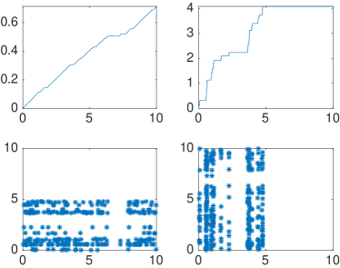
(a) $\alpha_{1}=0.95$, $\alpha_{2}=0.5$, $\lambda=100$

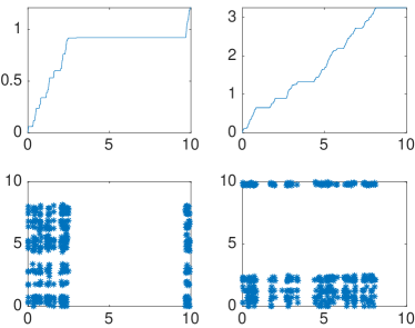
(b) $\alpha_{1}=\alpha_{2}=0.75$, $\lambda=100$

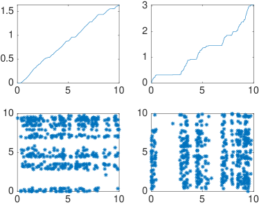
(c) $\alpha_{1}=0.9$, $\alpha_{2}=0.75$, $\lambda=100$

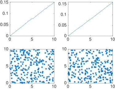
(d) $\alpha_{1}=\alpha_{2}\sim 1$, $\lambda=10000$

Figure 1: Simulations of the inverse stable subordinators $Y_{\alpha_{1}}^{(1)}(t)$ and $Y_{\alpha_{2}}^{(2)}(t)$ and the corresponding FPRF $N_{\alpha_{1},\alpha_{2}}$ for different values of $\alpha_{1}$ and $\alpha_{2}$. Top-left: simulation of $Y_{\alpha_{1}}^{(1)}(t)$, top-right: simulation of $Y_{\alpha_{2}}^{(2)}(t)$, bottom-(left-right): simulation of $N_{\alpha_{1},\alpha_{2}}$, the rotation shows the connection with marginal intensity

The subordinators $L_{\alpha}$ are simulated exactly at times $t_{n}=n\Delta$, where $\Delta=0.0005$ till they reach a defined value $S_{\mathrm{end}}$. More precisely,

$$L_{\alpha}(0)=0;\qquad L_{\alpha}(t_{n})=L_{\alpha}(t_{n-1})+X,\qquad n=1,2,\ldots,N$$

where $X$ is independently simulated with stblrnd($\alpha$, 1, $\sqrt[\alpha]{\Delta}$ , 0). Accordingly,

$$\mathrm{E}e^{-sX}=\exp\{-(s\sqrt[\alpha]{\Delta})^{\alpha}\}=\exp\{-\Delta s^{\alpha}\},\qquad s\geq 0,$$

and hence

$$\mathrm{E}e^{-sL_{\alpha}(t_{n})}=\exp\{-t_{n}s^{\alpha}\},\qquad s\geq 0,n=0,1,\ldots,N.$$

The simulation of the inverse stable subordinators $Y_{\alpha}(s),s\in[0,T_{\mathrm{end}}]$ are thus made at times $s_{n}=L_{\alpha}(t_{n}),n=1,\ldots,N$ with values $Y_{\alpha}(s_{n})=n\Delta$.

To simulate a FPRF $N_{\alpha_{1},\alpha_{2}}(s^{1},s^{2})$ on the window $(0,S_{\mathrm{end}})\times(0,S_{\mathrm{end}})$, we first simulate two independent inverse stable subordinators $Y_{\alpha_{1}}^{(1)}(s^{1}_{n}),n=1,\ldots,N_{1}$ and $Y_{\alpha_{2}}^{(2)}(s^{2}_{n}),n=1,\ldots,N_{2}$.

By Proposition 4.2, the value of $N_{\alpha_{1},\alpha_{2}}$ on each rectangle $(s^{1}_{n},s^{1}_{n+1})\times(s^{1}_{n},s^{1}_{n+1})$ is a Poisson random variable with mean $\Delta^{2}$. As $\Delta^{2}\ll 1$, we approximate it with a Bernoulli random variable $Y$ of parameter $\Delta^{2}$. When $Y=1$, we add a point at random inside the rectangle.

In Figure 1 the simulations of the inverse stable subordinators $Y_{\alpha_{1}}^{(1)}(t)$ and $Y_{\alpha_{2}}^{(2)}(t)$ and the corresponding FPRF $N_{\alpha_{1},\alpha_{2}}$ for different values of $\alpha_{1}$ and $\alpha_{2}$ are shown. The simulations of $N_{\alpha_{1},\alpha_{2}}$ are plotted twice: we have rotated each figure in order to underline the spatial dependence of the spread of the points of the process $N_{\alpha_{1},\alpha_{2}}$ in connection with the marginal intensities $Y_{\alpha_{1}}^{(1)}(t)$ and $Y_{\alpha_{2}}^{(2)}(t)$. For example, in Figure 1(c) two different marginal distribution are expected since $\alpha_{1}=0.9$ and $\alpha_{2}=0.75$. While $Y_{0.9}^{(1)}(t)$ produces a quite uniform distribution of points, $Y_{0.75}^{(2)}(t)$ generates clusters in correspondence of its steeper slopes.

We also compute the quantity

$$\mathrm{P}\left(N(Y_{1}(t_{1}),Y_{2}(t_{2}))=k\right)=\int_{0}^{\infty}\int_{0}^{\infty}\frac{e^{-\lambda x_{1}x_{2}}(\lambda x_{1}x_{2})^{k}}{k!}f_{\alpha_{1}}(t_{1},x_{1})f_{\alpha_{2}}(t_{2},x_{2})dx_{1}dx_{2},$$

given in (4.2), for different values of $t_{1},t_{2},\alpha_{1}$ and $\alpha_{2}$. In fact, with a Monte Carlo procedure, we approximate the above quantity with

$$\frac{1}{N^{2}}\sum_{n_{1}=1}^{N}\sum_{n_{2}=1}^{N}\frac{e^{-\lambda x_{1}x_{2}}(\lambda x_{1}x_{2})^{k}}{k!}{\mathbbm{1}}_{X_{n_{1}}}(x_{1}){\mathbbm{1}}_{Y_{n_{2}}}(x_{2})$$

where $(X_{n},n=1,\ldots,N)$ and $(Y_{n},n=1,\ldots,N)$ are independent sequences of i.i.d. distributed as $Y_{\alpha_{1}}^{(1)}(t_{1})$ and $Y_{\alpha_{2}}^{(2)}(t_{2})$, respectively. Summing up, the integral in (4.2) is computed numerically, and the simulations with $N=1500$ are presented in Figure 2. We underline the variety of the shape of distributions that can be generated with this two-parameter model in addition to its flexibility to include, for example, different cluster phenomena.

(a) $t_{1}=t_{2}=5$, $\alpha_{1}=0.5$, $\alpha_{2}=.75$

(b) $t_{1}=t_{2}=5$, $\alpha_{1}=0.95$, $\alpha_{2}=.075$

(c) $t_{1}=t_{2}=5$, $\alpha_{1}=\alpha_{2}=0.75$

(d) $t_{1}=3$, $t_{2}=7$, $\alpha_{1}=\alpha_{2}=0.75$

Figure 2: Simulations of the distribution of $Y_{\alpha_{1}}^{(1)}(t_{1})$, $Y_{\alpha_{2}}^{(2)}(t_{2})$ and the corresponding $p_{k}(t_{1},t_{2})=\mathrm{P}\left(N(Y_{1}(t_{1}),Y_{2}(t_{2}))=k\right)$ for $\lambda=10$ and different values of $t_{1},t_{2},\alpha_{1}$ and $\alpha_{2}$.

Appendix A Covariance Structure of Parameter-Changed Poisson random fields

In this Appendix, we prove a general result that can be used to compute the covariance structure of the parameter-changed Poisson random field:

$$Z\left(t_{1},t_{2}\right)=N(Y_{1}(t_{1}),Y_{2}(t_{2})),\ (t_{1},t_{2})\in\mathbb{R}_{+}^{2},$$

where $Y_{1}=\left\{Y_{1}(t_{1}),t_{1}\geq 0\right\}$ and $Y_{2}=\left\{Y_{2}(t_{2}),t_{2}\geq 0\right\}$ are independent non-negative non-decreasing stochastic processes, in general non-Markovian with non-stationary and non-independent increments, and $N=\{N(t_{1},t_{2}),(t_{1},t_{2})\in\mathbb{R}_{+}^{2}\}$ is a PRF with intensity $\lambda>0$. We also assume that $Y_{1}$ and $Y_{2}$ are independent of $N.$

For example, $Y_{1}$ and $Y_{2}$ might be inverse subordinators.

Theorem A.1.

Suppose that $N$ is a PRF, $Y_{1}$ and $Y_{2}$ are two non-decreasing non-negative independent stochastic processes which are also independent of $N.$ Then

1) if $\mathrm{E}Y_{1}(t_{1})=U_{1}(t_{1})$ and $\mathrm{E}Y_{2}(t_{2})=U_{2}(t_{2})$ exist, then $\mathrm{E}Z(t_{1},t_{2})$ exists and

$$\mathrm{E}Z(t_{1},t_{2})=\mathrm{E}N(1,1)\mathrm{E}Y_{1}(t_{1})\mathrm{E}Y_{2}(t_{2});$$

2) if $Y_{1}$ and $Y_{2}$ have second moments, so does $Z$ and

$$\mathrm{Var}Z(t_{1},t_{2})=\left[\mathrm{E}N(1,1)\right]^{2}\left\{\mathrm{E}Y_{1}^{2}(t_{1})\mathrm{E}Y_{2}^{2}(t_{2})-\left(\mathrm{E}Y_{1}(t_{1})\right)^{2}\left(\mathrm{E}Y_{2}(t_{2})\right)^{2}\right\}$$

$$+\mathrm{Var}N(1,1)\mathrm{E}Y_{1}(t_{1})\mathrm{E}Y_{2}(t_{2})$$

and its covariance function

$$\mathrm{Cov}(Z(t_{1},t_{2}),Z(s_{1},s_{2}))=\mathrm{Cov}\left(N(Y_{1}(t_{1}),Y_{2}(t_{2})),N(Y_{1}(s_{1}),Y_{2}(s_{2}))\right)$$

for $s_{1}<t_{1},s_{2}<t_{2}$ is given by:

$$(\mathrm{E}N(1,1))^{2}\Big{\{}\mathrm{Cov}\left(Y_{1}(t_{1}),Y_{1}(s_{1})\right)\mathrm{Cov}\left(Y_{2}(t_{2}),Y_{2}(s_{2})\right)\\ +\mathrm{E}Y_{2}(t_{2})\mathrm{E}Y_{2}(s_{2})\mathrm{Cov}\left(Y_{1}(t_{1}),Y_{1}(s_{1})\right)+\mathrm{E}Y_{1}(t_{1})\mathrm{E}Y_{1}(s_{1})\mathrm{Cov}\left(Y_{2}(t_{2}),Y_{2}(s_{2})\right)\Big{\}}\\ +\mathrm{Var}N(1,1)\mathrm{E}Y_{1}(s_{1})\mathrm{E}Y_{2}(s_{2})$$ (A.1)

and for any $(s_{1},s_{2}),$ and $(t_{1},t_{2})$ from $\mathbb{R}_{+}^{2}$

$$(\mathrm{E}N(1,1))^{2}\Big{\{}\mathrm{Cov}\left(Y_{1}(t_{1}),Y_{1}(s_{1})\right)\mathrm{Cov}\left(Y_{2}(t_{2}),Y_{2}(s_{2})\right)\\ +\mathrm{E}Y_{2}(t_{2})\mathrm{E}Y_{2}(s_{2})\mathrm{Cov}\left(Y_{1}(t_{1}),Y_{1}(s_{1})\right)+\mathrm{E}Y_{1}(t_{1})\mathrm{E}Y_{1}(s_{1})\mathrm{Cov}\left(Y_{2}(t_{2}),Y_{2}(s_{2})\right)\Big{\}}\\ +\mathrm{Var}N(1,1)\mathrm{E}Y_{1}(\min(s_{1},t_{1}))\mathrm{E}Y_{2}(\min(s_{2},t_{2}))$$ (A.2)

Remark.

These formulae are valid for any Lévy random field $N=\{N(t_{1},t_{2})$,$(t_{1},t_{2})\in\mathbb{R}_{+}^{2}\}$, with finite expectation $\mathrm{E}N(1,1)$ and finite variance $\mathrm{Var}N(1,1),$ for PRF $\mathrm{E}N(1,1)=\lambda;\ \mathrm{Var}N(1,1)=\lambda$ and to apply these formulae one needs to know

$$U_{1}(t_{1})=\mathrm{E}Y_{1}(t),\ U_{2}(t_{2})=\mathrm{E}Y_{2}(t),\ U_{1}^{(2)}(t_{1})=\mathrm{E}Y_{1}^{2}(t),~{}U_{2}^{(2)}(t_{1})=\mathrm{E}Y_{2}^{2}(t),\$$

and $\mathrm{Cov}\left(Y_{1}(t_{1}),Y_{1}(s_{1})\right),\ \mathrm{Cov}\left(Y_{2}(t_{2}),Y_{2}(s_{2})\right)$ which are available for many non-negative processes $Y_{1}(t)$ and $Y_{2}(t)$ induction inverse subordinators.

Remark.

One can compute the following expression for the one-dimensional distribution of the parameter-changed PRF:

$$\mathrm{P}\left(N(Y_{1}(t_{1}),Y_{2}(t_{2}))=k\right)=p_{k}(t_{1},t_{2})\\ =\int_{0}^{\infty}\int_{0}^{\infty}\frac{e^{-\lambda x_{1}x_{2}}(\lambda x_{1}x_{2})^{k}}{k!}f_{1}(t_{1},x_{1})f_{2}(t_{2},x_{2})dx_{1}dx_{2},\ k=0,1,2,\ldots$$

where

$$f_{i}(t_{i},x_{i})=\frac{d}{d{x_{i}}}\mathrm{P}\left\{Y_{i}(t_{i})\leq x_{i}\right\}=\frac{d}{dx_{i}}G_{t_{i}}^{(i)}(x_{i}),\qquad i=1,2.$$

and its Laplace transform:

$$\mathcal{L}\left\{p_{k}(t_{1},t_{2});s_{1},s_{2}\right\}=\int_{0}^{\infty}\int_{0}^{\infty}\frac{e^{-\lambda x_{1}x_{2}}(\lambda x_{1}x_{2})^{k}}{k!}\mathcal{L}\left\{f_{1}(t_{1},x_{1});s_{1}\right\}\mathcal{L}\left\{f_{2}(t_{2},x_{2});s_{2}\right\}dx_{1}dx_{2},$$

where

$$\mathcal{L}\left\{f_{i}(t_{i},x_{i});s_{i}\right\}=\int_{0}^{\infty}e^{-s_{i}t_{i}}f_{i}(t_{i},x_{i})dt_{i},\qquad i=1,2.$$

Proof of Theorem A.1.

We denote

$$G_{t_{1}}^{(1)}(u_{1})=\mathrm{P}\left\{Y_{1}(t_{1})\leq u_{1}\right\}, G_{t_{2}}^{(2)}(u_{2})=\mathrm{P}\left\{Y_{2}(t_{2})\leq u_{2}\right\}.$$

We know that for a PRF

$$\mathrm{E}\Delta_{s_{1},s_{2}}N(t_{1},t_{2})=\mathrm{E}N(1,1)\left(t_{1}-s_{1}\right)\left(t_{2}-s_{2}\right)=\mathrm{Var}\Delta_{s_{1},s_{2}}N(t_{1},t_{2});$$

$$\mathrm{E}\left(\Delta_{s_{1},s_{2}}N(t_{1},t_{2})\right)^{2}=\mathrm{E}N(1,1)\left(t_{1}-s_{1}\right)\left(t_{2}-s_{2}\right)+\left[\mathrm{E}N(1,1)\left(t_{1}-s_{1}\right)\left(t_{2}-s_{2}\right)\right]^{2}.$$

To prove 1) we use simple conditioning arguments:

$$\mathrm{E}Z(t_{1},t_{2})=\int_{0}^{\infty}\int_{0}^{\infty}u\ v\ \mathrm{E}N(1,1)G_{t_{1}}^{(1)}(du)G_{t_{2}}^{(2)}(dv)=\mathrm{E}N(1,1)\mathrm{E}Y_{1}(t_{1})\mathrm{E}Y_{2}(t_{2}).$$

Let us prove 2).

For the variance, we have

$$\mathrm{Var}Z(t_{1},t_{2}) = \mathrm{E}\left(N(Y_{1}(t_{1}),Y_{2}(t_{2})\right)^{2}-\left(\mathrm{E}N(Y_{1}(t_{1}),Y_{2}(t_{2})\right)^{2}$$

$$= \int_{0}^{\infty}\int_{0}^{\infty}\left((\mathrm{E}N(u_{1},u_{2}))^{2}+\mathrm{Var}N(u_{1},u_{2})\right)G_{t_{1}}^{(1)}(du_{1})G_{t_{2}}^{(2)}(du_{2})$$

$$-\left(\mathrm{E}N(1,1)\mathrm{E}Y_{1}(t_{1})\mathrm{E}Y_{2}(t_{2})\right)^{2}$$

$$= \int_{0}^{\infty}\int_{0}^{\infty}\left[\left(\mathrm{E}N(1,1)\right)^{2}u_{1}^{2}u_{2}^{2}+\mathrm{Var}N(1,1)u_{1}u_{2}\right]G_{t_{1}}^{(1)}(du_{1})G_{t_{2}}^{(2)}(du_{2})$$

$$-\left(\mathrm{E}N(1,1)\mathrm{E}Y_{1}(t_{1})\mathrm{E}Y_{2}(t_{2})\right)^{2}$$

$$= \left(\mathrm{E}N(1,1)\right)^{2}\mathrm{E}Y_{1}^{2}(t_{1})\mathrm{E}Y_{2}^{2}(t_{2})+\mathrm{Var}N(1,1)\mathrm{E}Y_{1}(t_{1})\mathrm{E}Y_{2}(t_{2})$$

$$-\left(\mathrm{E}N(1,1)\mathrm{E}Y_{1}(t_{1})\mathrm{E}Y_{2}(t_{2})\right)^{2}$$

$$= \left(\mathrm{E}N(1,1)\right)^{2}\left\{\mathrm{E}Y_{1}^{2}(t_{1})\mathrm{E}Y_{2}^{2}(t_{2})-(\mathrm{E}Y_{1}(t_{1}))^{2}(\mathrm{E}Y_{2}(t_{2}))^{2}\right\}$$

$$+\mathrm{Var}N(1,1)\mathrm{E}Y_{1}(t_{1})\mathrm{E}Y_{2}(t_{2}).$$

To compute the covariance structure, first we consider the case when $s_{1}<t_{1},\ s_{2}<t_{2}$. Then

$$\mathrm{E}N(s_{1},s_{2})N(t_{1},t_{2})$$

$$=\mathrm{E}\Big{(}N(s_{1},s_{2})\Big{\{}N(t_{1},t_{2})-N(t_{1},s_{2})-N(s_{1},t_{2})+N(s_{1},s_{2})$$

$$\qquad\qquad+N(t_{1},s_{2})+N(s_{1},t_{2})-N(s_{1},s_{2})\Big{\}}\Big{)}$$

$$=\mathrm{E}\Delta_{s_{1},s_{2}}N(t_{1},t_{2})\mathrm{E}N(s_{1},s_{2})+\mathrm{E}N(t_{1},s_{2})N(s_{1},s_{2})+\mathrm{E}N(s_{1},t_{2})N(s_{1},s_{2})-\mathrm{E}N^{2}(s_{1},s_{2}).$$

Using the facts that

$$\mathrm{E}\Delta_{s_{1},s_{2}}N(t_{1},t_{2})\mathrm{E}N(s_{1},s_{2})=(t_{1}-s_{1})(t_{2}-s_{2})\left[\mathrm{E}N(1,1)\right]^{2}s_{1}s_{2},$$

$$\begin{aligned} \mathrm{E}N(t_{1},s_{2})N(s_{1},s_{2})&=\mathrm{E}\{N(t_{1},s_{2})-N(s_{1},s_{2})+N(s_{1},s_{2})\}N(s_{1},s_{2})\\ &=\mathrm{E}\Delta_{s_{1},0}N(t_{1},s_{2})\mathrm{E}N(s_{1},s_{2})+\mathrm{E}N^{2}(s_{1},s_{2})\\ &=\left[\mathrm{E}N(1,1)\right]^{2}(t_{1}-s_{1})s_{1}s_{2}^{2}+\mathrm{E}N^{2}(s_{1},s_{2}),\end{aligned}$$

it is easy to obtain

$$\mathrm{E}N(s_{1},s_{2})N(t_{1},t_{2})=\left[\mathrm{E}N(1,1)\right]^{2}t_{1}t_{2}s_{1}s_{2}+s_{1}s_{2}\mathrm{Var}N(1,1).$$

Since the processes $N,Y_{1},Y_{2}$ are independent, a conditioning argument yields (A.1) and (A.2). In a similar way, one can consider the case $s_{1}>t_{1},s_{2}<t_{2}$. ∎

Proof of Proposition 4.1.

It follows from Theorem A.1 and Proposition 1.1. ∎

References

• [1] {barticle}[author] \bauthor\bsnmAletti, \bfnmGiacomo\binitsG. (\byear2001). \btitleOn different topologies for set-indexing collections. \bjournalStatist. Probab. Lett. \bvolume54 \bpages67–73. \bdoi10.1016/S0167-7152(01)00062-1 \bmrnumber1857872 (2002f:60064) \endbibitem
• [2] {barticle}[author] \bauthor\bsnmAletti, \bfnmG.\binitsG. and \bauthor\bsnmCapasso, \bfnmV.\binitsV. (\byear1999). \btitleCharacterization of spatial Poisson along optional increasing paths—a problem of dimension’s reduction. \bjournalStatist. Probab. Lett. \bvolume43 \bpages343–347. \bdoi10.1016/S0167-7152(98)00268-5 \bmrnumber1707943 (2000d:60084) \endbibitem
• [3] {barticle}[author] \bauthor\bsnmAletti, \bfnmG.\binitsG. and \bauthor\bsnmCapasso, \bfnmV.\binitsV. (\byear2002). \btitleReduction of dimension for spatial point processes and right continuous martingales. Characterization of spatial Poisson processes. \bjournalStoch. Stoch. Rep. \bvolume72 \bpages1–9. \bdoi10.1080/10451120212872 \bmrnumber1896435 (2003e:60101) \endbibitem
• [4] {bbook}[author] \bauthor\bsnmAndel, \bfnmJ.\binitsJ. (\byear2001). \btitleMathematics of Chance. \bseriesWiley Series in Probability and Statistics. \bpublisherWiley. \endbibitem
• [5] {barticle}[author] \bauthor\bsnmBeghin, \bfnmL.\binitsL. (\byear2012). \btitleRandom-time processes governed by differential equations of fractional distributed order. \bjournalChaos Solitons Fractals \bvolume45 \bpages1314–1327. \bdoi10.1016/j.chaos.2012.07.001 \bmrnumber2990245 \endbibitem
• [6] {barticle}[author] \bauthor\bsnmBeghin, \bfnmL.\binitsL. and \bauthor\bsnmOrsingher, \bfnmE.\binitsE. (\byear2009). \btitleFractional Poisson processes and related planar random motions. \bjournalElectron. J. Probab. \bvolume14 \bpages1790–1827. \bdoi10.1214/EJP.v14-675 \bmrnumber2535014 (2010m:60168) \endbibitem
• [7] {barticle}[author] \bauthor\bsnmBeghin, \bfnmL.\binitsL. and \bauthor\bsnmOrsingher, \bfnmE.\binitsE. (\byear2010). \btitlePoisson-type processes governed by fractional and higher-order recursive differential equations. \bjournalElectron. J. Probab. \bvolume15 \bpages684–709. \bdoi10.1214/EJP.v15-762 \bmrnumber2650778 (2011f:60168) \endbibitem
• [8] {barticle}[author] \bauthor\bsnmBingham, \bfnmN. H.\binitsN. H. (\byear1971). \btitleLimit theorems for occupation times of Markov processes. \bjournalZ. Wahrscheinlichkeitstheorie und Verw. Gebiete \bvolume17 \bpages1–22. \bdoi10.1007/BF00538470 \bmrnumber0281255 (43 ##6974) \endbibitem
• [9] {barticle}[author] \bauthor\bsnmBowsher, \bfnmClive G.\binitsC. G. and \bauthor\bsnmSwain, \bfnmPeter S.\binitsP. S. (\byear2012). \btitleIdentifying sources of variation and the flow of information in biochemical networks. \bjournalPNAS \bvolume109 \bpagesE1320-E1328. \bdoi10.1073/pnas.1119407109 \endbibitem
• [10] {bbook}[author] \bauthor\bsnmBrémaud, \bfnmPierre\binitsP. (\byear1981). \btitlePoint Processes and Queues. \bpublisherSpringer-Verlag, New York-Berlin. \bmrnumber636252 (82m:60058) \endbibitem
• [11] {barticle}[author] \bauthor\bsnmBusani, \bfnmOfer\binitsO. (\byear2016). \btitleAging uncoupled continuous time random walk limits. \bjournalElectron. J. Probab. \bvolume21 \bpagespaper no. 7, 17 pp. \bdoi10.1214/16-EJP3802 \endbibitem
• [12] {barticle}[author] \bauthor\bsnmCahoy, \bfnmDexter O.\binitsD. O., \bauthor\bsnmUchaikin, \bfnmVladimir V.\binitsV. V. and \bauthor\bsnmWoyczynski, \bfnmWojbor A.\binitsW. A. (\byear2010). \btitleParameter estimation for fractional Poisson processes. \bjournalJournal of Statistical Planning and Inference \bvolume140 \bpages3106 - 3120. \bdoihttps://doi.org/10.1016/j.jspi.2010.04.016 \endbibitem
• [13] {barticle}[author] \bauthor\bsnmCairoli, \bfnmR.\binitsR. and \bauthor\bsnmWalsh, \bfnmJohn B.\binitsJ. B. (\byear1975). \btitleStochastic integrals in the plane. \bjournalActa Math. \bvolume134 \bpages111–183. \bmrnumber0420845 (54 ##8857) \endbibitem
• [14] {barticle}[author] \bauthor\bsnmDaley, \bfnmD. J.\binitsD. J. (\byear1999). \btitleThe Hurst index of long-range dependent renewal processes. \bjournalAnn. Probab. \bvolume27 \bpages2035–2041. \bdoi10.1214/aop/1022677560 \bmrnumber1742900 (2000k:60175) \endbibitem
• [15] {barticle}[author] \bauthor\bsnmGergely, \bfnmT.\binitsT. and \bauthor\bsnmYezhow, \bfnmI. I.\binitsI. I. (\byear1973). \btitleOn a construction of ordinary Poisson processes and their modelling. \bjournalZ. Wahrscheinlichkeitstheorie und Verw. Gebiete \bvolume27 \bpages215–232. \bdoi10.1007/BF00535850 \bmrnumber0359012 (50 ##11467) \endbibitem
• [16] {barticle}[author] \bauthor\bsnmHaubold, \bfnmH. J.\binitsH. J., \bauthor\bsnmMathai, \bfnmA. M.\binitsA. M. and \bauthor\bsnmSaxena, \bfnmR. K.\binitsR. K. (\byear2011). \btitleMittag-Leffler functions and their applications. \bjournalJ. Appl. Math. \bpagesArt. ID 298628, 51. \bdoi10.1155/2011/298628 \bmrnumber2800586 (2012e:33061) \endbibitem
• [17] {barticle}[author] \bauthor\bsnmHerbin, \bfnmErick\binitsE. and \bauthor\bsnmMerzbach, \bfnmEly\binitsE. (\byear2013). \btitleThe set-indexed Lévy process: stationarity, Markov and sample paths properties. \bjournalStochastic Process. Appl. \bvolume123 \bpages1638–1670. \bdoi10.1016/j.spa.2013.01.001 \bmrnumber3027894 \endbibitem
• [18] {barticle}[author] \bauthor\bsnmIvanoff, \bfnmB. Gail\binitsB. G. and \bauthor\bsnmMerzbach, \bfnmEly\binitsE. (\byear1990). \btitleCharacterization of compensators for point processes on the plane. \bjournalStochastics Stochastics Rep. \bvolume29 \bpages395–405. \bdoi10.1080/17442509008833623 \endbibitem
• [19] {barticle}[author] \bauthor\bsnmIvanoff, \bfnmB. Gail\binitsB. G. and \bauthor\bsnmMerzbach, \bfnmEly\binitsE. (\byear1994). \btitleA martingale characterization of the set-indexed Poisson process. \bjournalStochastics Stochastics Rep. \bvolume51 \bpages69–82. \bdoi10.1080/17442509408833945 \bmrnumber1380763 (97c:60125) \endbibitem
• [20] {barticle}[author] \bauthor\bsnmIvanoff, \bfnmB. Gail\binitsB. G. and \bauthor\bsnmMerzbach, \bfnmEly\binitsE. (\byear2006). \btitleWhat is a multi-parameter renewal process? \bjournalStochastics \bvolume78 \bpages411–441. \bdoi10.1080/17442500600965239 \bmrnumber2281679 (2008h:60354) \endbibitem
• [21] {barticle}[author] \bauthor\bsnmIvanoff, \bfnmB. Gail\binitsB. G., \bauthor\bsnmMerzbach, \bfnmEly\binitsE. and \bauthor\bsnmPlante, \bfnmMathieu\binitsM. (\byear2007). \btitleA compensator characterization of point processes on topological lattices. \bjournalElectron. J. Probab. \bvolume12 \bpages47–74. \bdoi10.1214/EJP.v12-390 \bmrnumber2280258 (2008h:60187) \endbibitem
• [22] {bbook}[author] \bauthor\bsnmIvanoff, \bfnmGail\binitsG. and \bauthor\bsnmMerzbach, \bfnmEly\binitsE. (\byear2000). \btitleSet-Indexed Martingales. \bseriesMonographs on Statistics and Applied Probability \bvolume85. \bpublisherChapman & Hall/CRC, Boca Raton, FL. \bmrnumber1733295 (2001g:60105) \endbibitem
• [23] {bbook}[author] \bauthor\bsnmKallenberg, \bfnmOlav\binitsO. (\byear2002). \btitleFoundations of modern probability, \beditionsecond ed. \bseriesProbability and its Applications (New York). \bpublisherSpringer-Verlag, New York. \bmrnumber1876169 \endbibitem
• [24] {barticle}[author] \bauthor\bsnmKrengel, \bfnmUlrich\binitsU. and \bauthor\bsnmSucheston, \bfnmLouis\binitsL. (\byear1981). \btitleStopping rules and tactics for processes indexed by a directed set. \bjournalJ. Multivariate Anal. \bvolume11 \bpages199–229. \bdoi10.1016/0047-259X(81)90109-3 \bmrnumber618785 \endbibitem
• [25] {barticle}[author] \bauthor\bsnmLaskin, \bfnmNick\binitsN. (\byear2003). \btitleFractional Poisson process. \bjournalCommunications in Nonlinear Science and Numerical Simulation \bvolume8 \bpages201-213. \bdoi10.1016/S1007-5704(03)00037-6 \endbibitem
• [26] {barticle}[author] \bauthor\bsnmLeonenko, \bfnmNikolai\binitsN. and \bauthor\bsnmMerzbach, \bfnmEly\binitsE. (\byear2015). \btitleFractional Poisson fields. \bjournalMethodol. Comput. Appl. Probab. \bvolume17 \bpages155–168. \bdoi10.1007/s11009-013-9354-7 \bmrnumber3306677 \endbibitem
• [27] {barticle}[author] \bauthor\bsnmLeonenko, \bfnmNikolai\binitsN., \bauthor\bsnmScalas, \bfnmEnrico\binitsE. and \bauthor\bsnmTrinh, \bfnmMailan\binitsM. (\byear2017). \btitleThe fractional non-homogeneous Poisson process. \bjournalStatist. Probab. Lett. \bvolume120 \bpages147–156. \bdoi10.1016/j.spl.2016.09.024 \bmrnumber3567934 \endbibitem
• [28] {barticle}[author] \bauthor\bsnmLeonenko, \bfnmNikolai N.\binitsN. N., \bauthor\bsnmMeerschaert, \bfnmMark M.\binitsM. M., \bauthor\bsnmSchilling, \bfnmRené L.\binitsR. L. and \bauthor\bsnmSikorskii, \bfnmAlla\binitsA. (\byear2014). \btitleCorrelation structure of time-changed Lévy processes. \bjournalCommun. Appl. Ind. Math. \bvolume6 \bpagese-483, 22 pp. \bdoi10.1685/journal.caim.483 \bmrnumber3277310 \endbibitem
• [29] {barticle}[author] \bauthor\bsnmLeonenko, \bfnmNikolai N.\binitsN. N., \bauthor\bsnmMeerschaert, \bfnmMark M.\binitsM. M. and \bauthor\bsnmSikorskii, \bfnmAlla\binitsA. (\byear2013). \btitleFractional Pearson diffusions. \bjournalJ. Math. Anal. Appl. \bvolume403 \bpages532–546. \bdoi10.1016/j.jmaa.2013.02.046 \bmrnumber3037487 \endbibitem
• [30] {barticle}[author] \bauthor\bsnmLeonenko, \bfnmN. N.\binitsN. N., \bauthor\bsnmRuiz-Medina, \bfnmM. D.\binitsM. D. and \bauthor\bsnmTaqqu, \bfnmM. S.\binitsM. S. (\byear2011). \btitleFractional elliptic, hyperbolic and parabolic random fields. \bjournalElectron. J. Probab. \bvolume16 \bpages1134–1172. \bdoi10.1214/EJP.v16-891 \bmrnumber2820073 (2012m:60112) \endbibitem
• [31] {barticle}[author] \bauthor\bsnmMagdziarz, \bfnmMarcin\binitsM. (\byear2010). \btitlePath properties of subdiffusion—a martingale approach. \bjournalStoch. Models \bvolume26 \bpages256–271. \bdoi10.1080/15326341003756379 \bmrnumber2739351 \endbibitem
• [32] {barticle}[author] \bauthor\bsnmMainardi, \bfnmFrancesco\binitsF., \bauthor\bsnmGorenflo, \bfnmRudolf\binitsR. and \bauthor\bsnmScalas, \bfnmEnrico\binitsE. (\byear2004). \btitleA fractional generalization of the Poisson processes. \bjournalVietnam J. Math. \bvolume32 \bpages53–64. \bmrnumber2120631 \endbibitem
• [33] {barticle}[author] \bauthor\bsnmMainardi, \bfnmFrancesco\binitsF., \bauthor\bsnmGorenflo, \bfnmRudolf\binitsR. and \bauthor\bsnmVivoli, \bfnmAlessandro\binitsA. (\byear2005). \btitleRenewal processes of Mittag-Leffler and Wright type. \bjournalFract. Calc. Appl. Anal. \bvolume8 \bpages7–38. \bmrnumber2179226 \endbibitem
• [34] {barticle}[author] \bauthor\bsnmMeerschaert, \bfnmMark M.\binitsM. M., \bauthor\bsnmNane, \bfnmErkan\binitsE. and \bauthor\bsnmVellaisamy, \bfnmP.\binitsP. (\byear2011). \btitleThe fractional Poisson process and the inverse stable subordinator. \bjournalElectron. J. Probab. \bvolume16 \bpages1600–1620. \bdoi10.1214/EJP.v16-920 \bmrnumber2835248 (2012k:60252) \endbibitem
• [35] {barticle}[author] \bauthor\bsnmMeerschaert, \bfnmMark M.\binitsM. M. and \bauthor\bsnmScheffler, \bfnmHans-Peter\binitsH.-P. (\byear2008). \btitleTriangular array limits for continuous time random walks. \bjournalStochastic Process. Appl. \bvolume118 \bpages1606–1633. \bdoi10.1016/j.spa.2007.10.005 \bmrnumber2442372 (2010b:60135) \endbibitem
• [36] {bbook}[author] \bauthor\bsnmMeerschaert, \bfnmMark M.\binitsM. M. and \bauthor\bsnmSikorskii, \bfnmAlla\binitsA. (\byear2012). \btitleStochastic Models for Fractional Calculus. \bseriesde Gruyter Studies in Mathematics \bvolume43. \bpublisherWalter de Gruyter & Co., Berlin. \bmrnumber2884383 \endbibitem
• [37] {barticle}[author] \bauthor\bsnmMerzbach, \bfnmEly\binitsE. and \bauthor\bsnmNualart, \bfnmDavid\binitsD. (\byear1986). \btitleA characterization of the spatial Poisson process and changing time. \bjournalAnn. Probab. \bvolume14 \bpages1380–1390. \bdoi10.1214/aop/1176992378 \bmrnumber866358 (88d:60145) \endbibitem
• [38] {barticle}[author] \bauthor\bsnmMerzbach, \bfnmEly\binitsE. and \bauthor\bsnmShaki, \bfnmYair Y.\binitsY. Y. (\byear2008). \btitleCharacterizations of multiparameter Cox and Poisson processes by the renewal property. \bjournalStatist. Probab. Lett. \bvolume78 \bpages637–642. \bdoi10.1016/j.spl.2007.09.026 \bmrnumber2409527 (2009d:60151) \endbibitem
• [39] {btechreport}[author] \bauthor\bsnmMijena, \bfnmJebessa B.\binitsJ. B. (\byear2014). \btitleCorrelation structure of time-changed fractional Brownian motion \btypearXiv:1408.4502. \endbibitem
• [40] {barticle}[author] \bauthor\bsnmNane, \bfnmErkan\binitsE. and \bauthor\bsnmNi, \bfnmYinan\binitsY. (\byear2017). \btitleStability of the solution of stochastic differential equation driven by time-changed Lévy noise. \bjournalProc. Amer. Math. Soc. \bvolume145 \bpages3085–3104. \bmrnumber3637955 \endbibitem
• [41] {barticle}[author] \bauthor\bsnmPiryatinska, \bfnmA.\binitsA., \bauthor\bsnmSaichev, \bfnmA. I.\binitsA. I. and \bauthor\bsnmWoyczynski, \bfnmW. A.\binitsW. A. (\byear2005). \btitleModels of anomalous diffusion: The subdiffusive case. \bjournalPhysica A \bvolume349 \bpages375-420. \bdoi10.1016/j.physa.2004.11.003 \endbibitem
• [42] {bbook}[author] \bauthor\bsnmPodlubny, \bfnmIgor\binitsI. (\byear1999). \btitleFractional Differential Equations. \bseriesMathematics in Science and Engineering \bvolume198. \bpublisherAcademic Press, Inc., San Diego, CA. \bmrnumber1658022 (99m:26009) \endbibitem
• [43] {barticle}[author] \bauthor\bsnmPolito, \bfnmFederico\binitsF. and \bauthor\bsnmScalas, \bfnmEnrico\binitsE. (\byear2016). \btitleA generalization of the space-fractional Poisson process and its connection to some Lévy processes. \bjournalElectron. Commun. Probab. \bvolume21 \bpages14 pp. \bdoi10.1214/16-ECP4383 \endbibitem
• [44] {barticle}[author] \bauthor\bsnmRepin, \bfnmO. N.\binitsO. N. and \bauthor\bsnmSaichev, \bfnmA. I.\binitsA. I. (\byear2000). \btitleFractional Poisson law. \bjournalRadiophys. and Quantum Electronics \bvolume43 \bpages738–741. \bdoi10.1023/A:1004890226863 \bmrnumber1910034 \endbibitem
• [45] {bbook}[author] \bauthor\bsnmRoss, \bfnmSheldon\binitsS. (\byear2011). \btitleA first course in probability, \beditionEight ed. \bpublisherMacmillan Co., New York; Collier Macmillan Ltd., London. \endbibitem
• [46] {barticle}[author] \bauthor\bsnmScalas, \bfnmE\binitsE., \bauthor\bsnmGorenflo, \bfnmR\binitsR. and \bauthor\bsnmMainardi, \bfnmF\binitsF. (\byear2004). \btitleUncoupled continuous-time random walks: Solution and limiting behavior of the master equation. \bjournalPhysical Review E \bvolume69. \bdoi10.1103/PhysRevE.69.011107 \endbibitem
• [47] {bbook}[author] \bauthor\bsnmStoyan, \bfnmD.\binitsD., \bauthor\bsnmKendall, \bfnmW. S.\binitsW. S. and \bauthor\bsnmMecke, \bfnmJ.\binitsJ. (\byear1987). \btitleStochastic Geometry and its Applications. \bseriesWiley Series in Probability and Mathematical Statistics: Applied Probability and Statistics. \bpublisherJohn Wiley & Sons, Ltd., Chichester \bnoteWith a foreword by D. G. Kendall. \bmrnumber895588 (88j:60034a) \endbibitem
• [48] {bbook}[author] \bauthor\bsnmUchaikin, \bfnmVladimir V.\binitsV. V. and \bauthor\bsnmZolotarev, \bfnmVladimir M.\binitsV. M. (\byear1999). \btitleChance and stability. \bseriesModern Probability and Statistics. \bpublisherVSP, Utrecht \bnoteStable distributions and their applications, With a foreword by V. Yu. Korolev and Zolotarev. \bdoi10.1515/9783110935974 \bmrnumber1745764 \endbibitem
• [49] {barticle}[author] \bauthor\bsnmVeillette, \bfnmMark\binitsM. and \bauthor\bsnmTaqqu, \bfnmMurad S.\binitsM. S. (\byear2010). \btitleNumerical computation of first passage times of increasing Lévy processes. \bjournalMethodol. Comput. Appl. Probab. \bvolume12 \bpages695–729. \bdoi10.1007/s11009-009-9158-y \bmrnumber2726540 (2012f:60150) \endbibitem
• [50] {barticle}[author] \bauthor\bsnmVeillette, \bfnmMark\binitsM. and \bauthor\bsnmTaqqu, \bfnmMurad S.\binitsM. S. (\byear2010). \btitleUsing differential equations to obtain joint moments of first-passage times of increasing Lévy processes. \bjournalStatist. Probab. Lett. \bvolume80 \bpages697–705. \bdoi10.1016/j.spl.2010.01.002 \bmrnumber2595149 (2011c:60129) \endbibitem
• [51] {barticle}[author] \bauthor\bsnmWatanabe, \bfnmShinzo\binitsS. (\byear1964). \btitleOn discontinuous additive functionals and Lévy measures of a Markov process. \bjournalJapan. J. Math. \bvolume34 \bpages53–70. \bmrnumber0185675 (32 ##3137) \endbibitem