Non-extensive condensation in reinforced branching processes

Abstract

We study a class of branching processes in which a population consists of immortal individuals equipped with a fitness value. Individuals produce offspring with a rate given by their fitness, and offspring may either belong to the same family, sharing the fitness of their parent, or be founders of new families, with a fitness sampled from a fitness distribution $\mu$. Examples that can be embedded in this class are stochastic house-of-cards models, urn models with reinforcement, and the preferential attachment tree of Bianconi and Barabási. Our focus is on the case when the fitness distribution $\mu$ has bounded support and regularly varying tail at the essential supremum. In this case there exists a condensation phase, in which asymptotically a proportion of mass in the empirical fitness distribution of the overall population condenses in the maximal fitness value. Our main results describe the asymptotic behaviour of the size and fitness of the largest family at a given time. In particular, we show that as time goes to infinity the size of the largest family is always negligible compared to the overall population size. This implies that condensation, when it arises, is non-extensive and emerges as a collective effort of several families none of which can create a condensate on its own. Our result disproves claims made in the physics literature in the context of preferential attachment trees.

Keywords: Network; preferential attachment; Bianconi-Barabási model; genetics; house-of-cards model; selection and mutation; urn model; reinforcement; non-Malthusian branching; Crump-Mode-Jagers process; condensation.
MSC Classification: Primary 60J80; Secondary 05C82; 60G70.

1 Background and motivation

The principal aim of this paper is to study the emergence of a condensate in stochastic models. For this purpose we consider a class of branching processes with reinforcement, which probably constitute the easiest class of models, in which this question can be studied in a meaningful way. Still we shall see that, due to the reinforcement, these models display rather complex behaviour and not all relevant questions on their behaviour will be answered.

Although our models can describe a variety of objects, see the examples below, we shall describe them as a structured population. Parameters of our model are a fitness distribution $\mu$ on the positive reals, and positive numbers $\beta,\gamma\leq 1$ with $\beta+\gamma\geq 1$. At any time $t$ the population consists of a finite number $N(t)$ of individuals. Each individual in the population has a fitness, and individuals are organised into families, such that all members of a family have the same fitness. The process is started with one family of one individual, whose fitness is drawn from the distribution $\mu$. Suppose, at time $t\geq 0$, the population consists of $M(t)$ families, and there are $Z_{n}(t)$ individuals of fitness $F_{n}$ in the $n$th family, for $1\leq n\leq M(t)$. Independently in every family birth events occur with a time-dependent rate $F_{n}Z_{n}(t)$. When a birth event occurs in the $n$th family, independently of everything else, one or both of the following happen,

• with probability $\beta$ a new family is founded, initially consisting of one individual equipped with a fitness drawn, independently of everything else, from the distribution $\mu$;

• with probability $\gamma$ a new individual with fitness $F_{n}$ is added to the $n$th family. The ability of the system to reproduce particles of the same type constitutes the reinforcement, see [21].

Note that both things happen simultaneously with probability $\beta+\gamma-1\geq 0$. If $\mu$ has all exponential moments the total number $N(t)$ of individuals in the population remains finite at all times, see for example Corollary 3.3 in [19]. Our main object of interest is the empirical fitness distribution at time $t$, which is defined as

$$\Xi_{t}=\frac{1}{N(t)}\sum_{n=1}^{M(t)}Z_{n}(t)\,\delta_{F_{n}}.$$ (1)

In this paper we focus on bounded fitness distributions $\mu$, and specifically the case in which a condensation phenomenon occurs, which we describe in some detail. Different phenomena occur in the case of unbounded fitness distributions and these will be investigated in a companion paper [11]. From now on we assume that $\mu$ is a probability measure supported by a bounded subinterval of the positive reals. Without loss of generality we assume that $\mu$ has essential supremum equal to one. To avoid degeneracies we also assume that $\mu$ has no atom at one.

We now describe our three main examples motivating our work.

Example 1: Branching process with selection and mutation.

This model is a stochastic house-of-cards model in a similar vein as Kingman’s model (which is deterministic and much easier to analyse, see [18, 12]). We start with a single individual with a genetic fitness chosen according to $\mu$. Individuals never die and give birth to new individuals with a rate equal to their genetic fitness, the different reproduction rates causing the selection effect. When a new individual is born it is a mutant with probability $\beta$, in which case it gets a fitness drawn independently of everything else from $\mu$. If the new individual is not a mutant, it inherits the fitness of its parent. The model corresponds to the parameter choice $\gamma=1-\beta$ in our framework. Observe that a mutation causes the complete loss of genetic information in the affected individual’s ancestry, pictorially speaking ‘the genetic house of cards collapses’. This is why the term house-of-cards model is used for this process, see [15] for a discussion of the relevance of these models in the theory of evolution.

The number of families $M(t)$ corresponds to the number of mutants in the population at time $t$. We can describe the process $(M(t))_{t>0}$ as a Crump-Mode-Jagers process, using the framework of [20]. A mutant $x$ born at time $\tau$ with fitness $f$ produces new mutants at ages according to a random point process $\xi$. This process is a Cox process, i.e. a Poisson process with a random intensity measure $\beta f\phi_{x}(s)\,ds$. The function $\phi_{x}(s)$ is given by the size at time $\tau+s$ of the family founded by the mutant and is therefore a Yule processes with intensity $(1-\beta)f$.

The key assumption for the convergence theory of Crump-Mode-Jagers processes is the existence of a Malthusian parameter, i.e. an $\alpha>0$ such that

$$1=\int_{0}^{\infty}e^{-\alpha s}\,{\mathbb{E}}\xi(ds).$$

In our case we have, for $\alpha\geq 1-\beta$, that

$$\int_{0}^{\infty}e^{-\alpha s}\,{\mathbb{E}}\xi(ds)={\mathbb{E}}\int_{0}^{\infty}e^{-\alpha s}\beta f\phi_{x}(s)\,ds=\beta\int f\int_{0}^{\infty}e^{-\alpha s+(1-\beta)fs}\,ds\,\mu(df)=\beta\int\frac{f}{\alpha-(1-\beta)f}\,\mu(df).$$

Hence a Malthusian parameter exists if and only if $\frac{\beta}{1-\beta}\int\frac{f}{1-f}\,\mu(df)\geq 1$. If this condition fails, the classical convergence theory of Crump-Mode-Jagers processes fails and very little is known about this case. In particular, in our model the precise asymptotics of $M(t)$ is unknown. We show that in this case a phenomenon of condensation occurs, which loosely speaking means that a positive proportion of individuals have fitnesses converging to the maximal possible value. Key questions motivating this project are: How fast is this convergence, when did the mutations arise that form the condensate, and how many mutations contribute to the condensate?

Example 2: Preferential attachment tree of Bianconi and Barabási.

This model is originally a discrete time network model. Putting it into our framework means embedding it into continuous time, a technique heavily advocated by Janson [16], who attributes the method to Athreya and Karlin [1], and by Bhamidi [6]. The network is constructed successively, starting with one vertex which is formally given degree one. The vertex is given a fitness, randomly chosen according to $\mu$. At every time step a new vertex is introduced, equipped with a fitness, randomly chosen according to $\mu$, and linked to one of the existing vertices. The probability of an existing vertex being chosen is proportional to the product of its fitness and its degree at the time when the new vertex is introduced. As new vertices prefer to attach to existing vertices of high degree and high fitness, this is called a preferential attachment model.

In our representation we choose $\beta=\gamma=1$ and observe the system at the birth times of individuals. We think of every family as a vertex in the network, and of the size of a family as its degree. Note that when the $n$th birth event takes place, it arises in each of the existing families with a probability proportional to the product of its fitness and its degree. At the birth event a new family is founded, i.e. a new vertex is introduced, and simultaneously the family that has given birth is increased in size by one, meaning that the degree of the corresponding vertex is incremented by one. Our representation only keeps track of the vertices and their degrees, not of the actual edges. But this does not matter as the main object of interest for us is the long-term behaviour of the degree-weighted fitness distribution, which coincides with the empirical fitness distribution in our framework.

This model was analysed by Borgs et al. [7] who proved the existence of a innovation-pays-off phase in which a proportion of the mass in the degree-weighted fitness distribution condenses in the maximal fitness. This behaviour was already predicted in [4] who called this phase the winner-takes-all phase, a heavily misleading name as we shall see below. The result is reproved in our Theorem 2.1. Borgs et al. [7] state as an open problem ‘to give an exact quantitative description of the innovation-pays-off phase. […] How are the links distributed among the highest fitnesses present in the system at any given time? At what rate are new nodes with higher fitness taking over?’ Our main aim here is to make progress on this problem.

Example 3: Generalised Pólya urns.

A class of generalised Pólya urns also falls into our framework, with general parameters $\beta,\gamma>0$ and $\mu$ as above. It can be described as an urn containing balls of different colours. Every colour has a given activity chosen independently according to $\mu$. At time zero, the urn contains one ball of colour $1$. At every time step, a ball is drawn at random from the urn with probability proportional to its activity. Then, the drawn ball is put back into the urn together with one or two new balls, at most one ball of the same and one of a new colour. A ball with the same colour is chosen with probability $\gamma$, and a ball of a new colour with probability $\beta$. New colours are chosen independently according to $\mu$. To embed the urn model into our framework we again look at the times of birth events. Observe that $\Xi_{t}$ is now the empirical distribution of activities in the urn at time $t$.

Such generalised Pólya urns have apparently not been studied so far in full generality. Janson [16] is looking at the case where $\mu$ is finitely supported, in which the condensation phenomenon, which is of interest to us, cannot arise. A related model has been studied by Chung et al. [8] who draw balls depending in a non-linear way on the distribution of colours in the urn, and by Collevecchio et al. [9] who allow for a time-dependent replacement rule. Their main focus is on the question whether there can be an unbounded number of balls of more than one colour, and if not which colour eventually dominates. In our setup all colours will have an unbounded number of balls and we show that the asymptotic proportion of balls of any colour goes to zero uniformly as time goes to infinity.

2 Statement of the results

The reinforced branching process is described by the following family of random variables. We denote by

• $N(t)$ the total size of the population at time $t$,

• $M(t)$ the number of different families at time $t$,

• $\sigma_{n}$ the time of the $n^{\text{th}}$ birth event,

• $\tau_{n}$ the time of the foundation of the $n^{\text{th}}$ family,

• $Z_{n}(t)$ the size of the $n^{\text{th}}$ family at time $t$ (if $n>M(t)$ we set $Z_{n}(t)=0$), and

• $F_{n}$ the fitness of the $n^{\text{th}}$ family.

We are first interested in the empirical fitness distribution $\Xi_{t}$ at time $t$, defined in (1). The asymptotic behaviour of this empirical distribution shows a phase transition between a fluid phase and a condensation phase. The condition for condensation is

$$\frac{\beta}{\beta+\gamma}\int_{0}^{1}\frac{1}{1-x}\,d\mu(x)<1\quad\mbox{ or, equivalently, }\quad\frac{\beta}{\gamma}\int_{0}^{1}\frac{x}{1-x}\,d\mu(x)<1,$$ (Cond)

as stated in the following theorem.

Theorem 2.1 (Existence of a condensation phase).

If (Cond) fails, then there exists a unique $\lambda^{\star}\in[\gamma,\beta+\gamma)$ such that

$$\frac{\beta}{\beta+\gamma}\int_{0}^{1}\frac{\lambda^{\star}}{\lambda^{\star}-\gamma x}\,d\mu(x)=1,$$

otherwise let $\lambda^{\star}:=\gamma$. In both cases

• the empirical mean fitness $\int_{0}^{1}x\,\Xi_{t}(dx)$ converges almost surely to $\nicefrac{{\lambda^{\star}}}{{\beta+\gamma}}$,

• and there exists a probability measure $\pi$ such that, almost surely, the empirical fitness distribution $\Xi_{t}$ converges weakly to $\pi$.

The limit measure $\pi$ of the empirical fitness distribution is given

• if (Cond) fails by

  $$d\pi(x)=\frac{\beta}{\beta+\gamma}\frac{\lambda^{\star}}{\lambda^{\star}-\gamma x}d\mu(x).$$

• if (Cond) is true by

  $$d\pi(x)={\frac{\beta}{\beta+\gamma}}\frac{1}{1-x}d\mu(x)+\omega(\beta,\gamma)\delta_{1}(dx),$$

  where

  $$\omega(\beta,\gamma):=1-\frac{\beta}{\beta+\gamma}\int_{0}^{1}\frac{1}{1-x}d\mu(x)>0.$$

Remark 1.

It is easy to see from the law of large numbers that

$$\frac{M(t)}{N(t)}\longrightarrow\frac{\beta}{\beta+\gamma}\qquad\mbox{ almost surely.}$$

Hence it is equivalent to ask for the absolute growth of either of the processes $(M(t)\colon t>0)$ or $(N(t)\colon t>0)$. Given the population at time $\sigma_{n}$ of the $n$th birth event, the waiting time $\sigma_{n+1}-\sigma_{n}$ until the next individual is born is exponentially distributed with rate $N(\sigma_{n})\int x\,\Xi_{\sigma_{n}}(dx)\sim n\lambda^{\star}$, where we have used that $N(\sigma_{n})\sim(\beta+\gamma)n$ by the law of large numbers. Hence $\sigma_{n}\sim\frac{1}{\lambda^{\star}}\log n$ and, in particular, we obtain, almost surely,

$$\lim_{t\uparrow\infty}\frac{1}{t}\log N(t)=\lambda^{\star}.$$

If there is no condensation we can improve this to convergence of $e^{-t\lambda^{\star}}N(t)$ to a positive random variable, using the arguments sketched in Section 3.2 below. But fine results about the growth of the population in the condensation phase are hard to obtain, see also Section 8 .

Remark 2.

We denote the part of the limit mass $\pi$ which is absolutely continuous with respect to $\mu$ as bulk and the part concentrated in the maximal fitness as condensate. The theorem shows that in the condensation phase, i.e. if (Cond) holds, we are seeing a phenomenon of self-organised criticality, as the number of individuals in the bulk and in the condensate are always kept on the same order of magnitude, without any tuning of parameters. In Dereich [10] one can see that for a model without self-organisation it can be rather complicated to tune the parameters in such a way that one has coexistence of bulk and condensate.

Our interest in this paper lies in the emergence of the condensate, i.e. how the condensate manifests itself at large finite times. Following the discussion of Bose-Einstein condensation in van den Berg et al. [3] two alternative scenarios are possible:

• For the largest family, the proportion of individuals belonging to this family in the overall population at time $t$ is asymptotically positive. This phenomenon of macroscopic occupancy arises in condensation of the free Bose gas below a critical temperature, see [3].

• No individual family makes an asymptotically positive contribution. Instead, it is a collective effort of a growing number of families to form the condensate. This phenomenon is called non-extensive condensation. van den Berg et al. [3] have shown that this occurs in the free Bose gas for an intermediate temperature range.

We shall see in Theorem 2.4 that in our model under a natural assumption on $\mu$ the second scenario prevails. To show this we need to investigate the behaviour of the largest family in our system. This requires some regularity assumptions on $\mu$. We henceforth assume that the fitness distribution $\mu$ has a regularly varying tail in one, meaning that there exists $\alpha>1$ and a slowly varying function $\ell$ with

$$\mu(1-\varepsilon,1)=\varepsilon^{\alpha}\ell(\varepsilon).$$ (RV)

This corresponds to the most common type of behaviour of $\mu$ at its tip that allows a condensation phase.

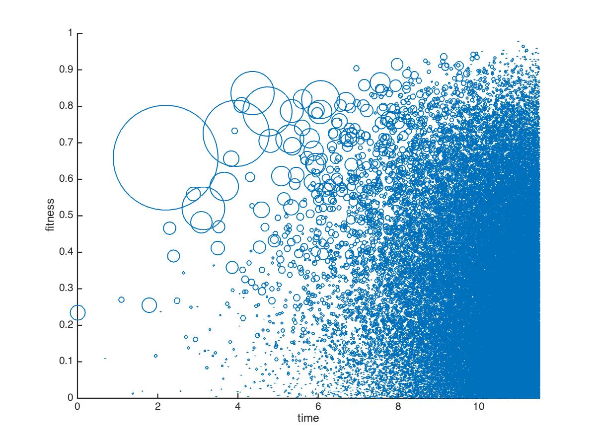
Figure 1: A simulation of a reinforced branching process in the condensation case. Parameters are $\mu(dx)=3(1-x)^{2}\,dx$ and $\beta=\gamma=1$. Each family is represented by a circle with area proportional to
its size at time $t=12$ and centred at its time of birth (horizontal axis) and its fitness (vertical axis).
Simulation courtesy of Anna Senkevich.

We start with a heuristic consideration. Suppose $t>0$ is given. At any time $s\in(0,t)$ there are $\exp((\lambda^{*}+o(1))s)$ families in the system and by an extreme value calculation the largest fitness in this number of families is of order $1-\exp(-(\frac{\lambda^{*}}{\alpha}+o(1))s)$. Until time $t>s$ the family achieving this fitness has time $t-s$ to grow and therefore has size of order $\exp(\gamma(t-s)(1-e^{-\frac{\lambda^{*}}{\alpha}s}))$. We therefore expect the birth time $s$ of the maximal family at time $t$ to be around the maximiser of this expression over $0<s<t.$ This maximum occurs roughly at time $s\sim\nicefrac{{\alpha}}{{\lambda^{\star}}}\log t$.

For the rigorous results we replace this time $s$ by the stopping time

$$T(t):=\inf\bigl{\{}s\geq 0\colon M(s)\geq n(t)\bigr{\}}\quad\text{where}\quad n(t):=\big{\lceil}\mbox{$\frac{1}{\mu(1-t^{-1},1)}$}\big{\rceil},$$

which allows us precise control over the number of families in the system. Note that $T(t)\sim\nicefrac{{\alpha}}{{\lambda^{\star}}}\log t$, as can be seen by putting $M(s)=\exp((\lambda^{*}+o(1))s)$ and $\log n(t)=(\alpha+o(1))\log t$. Our heuristics suggests that the dominant families of the population at time $t$ are born in a window around time $T(t)$, have fitness $F_{n}$ with $1-F_{n}$ of order $1/t$, and size of order $\exp(\gamma(t-T(t)))$.

To confirm this intuition we zoom into this window by considering the point process

$$\Gamma_{t}=\sum_{n=1}^{M(t)}\delta{\big{(}\tau_{n}-T(t),(t-\tau_{n})(1-F_{n}),e^{-\gamma(t-T(t))}Z_{n}(t)\big{)}},$$

where $\delta(x)$ is the Dirac mass in $x$.

Theorem 2.2 (Poisson limit).

Under assumption (RV) the point process $(\Gamma_{t})_{t\geq 0}$ converges vaguely on the space $[-\infty,\infty]\times[0,\infty]\times(0,\infty]$ to the Poisson point process with intensity measure

$$d\zeta(s,f,z)=\alpha f^{\alpha-1}\lambda^{\star}e^{\lambda^{\star}s}e^{-ze^{\gamma(s+f)}}e^{\gamma(s+f)}\,ds\,df\,dz.$$

Remark 3.

Note the compactifications at $\pm\infty$ in Theorem 2.2. As the limiting point process has a continuous density, Theorem 2.2 implies that all mass of $\Gamma_{t}$ that asymptotically accumulates at infinity in one of the first two components, must escape at zero in the last component, meaning that the only way points can disappear in the limit is because the corresponding family size is small relative to the normalisation.

Remark 4.

As there is no scaling in the first component of $\Gamma_{t}$, the limit theorem focuses on a time window of constant width around $T(t)$. The theorem shows that this is wide enough to capture the largest family at time $t$. However, it turns out that in the condensation phase this is not wide enough to capture all families that contribute to the condensate. This is why important questions on the emergence of the condensate remain open in this paper, see for example the first two problems in Section 8.

Our Poisson limit result, Theorem 2.2, readily implies the following distributional limits (denoted by $\Longrightarrow$) for the size, fitness and birth time of the largest family.

Corollary 2.3 (Limits of family characteristics).

1. Asymptotically, as $t\to\infty$,

   $$e^{-\gamma(t-T(t))}\max_{n\in\mathbb{N}}Z_{n}(t)\Longrightarrow W^{-\frac{\gamma}{\lambda^{\star}}},$$

   where $W$ is exponentially distributed with parameter $\Gamma(\alpha+1)\Gamma(1+\frac{\lambda^{\star}}{\gamma})(\lambda^{\star})^{-\alpha}$.

2. Under (Cond), denoting by $V(t)$ the fitness of the family of maximal size at time $t$, as $t\to\infty$, we have

   $$t(1-V(t))\Longrightarrow V,$$

   where $V$ is Gamma-distributed with scale parameter $\lambda^{\star}$ and shape parameter $\alpha$.

3. Denoting by $S(t)$ the birth time of the family of maximal size at time $t$, as $t\to\infty$, we have

   $$S(t)-T(t)\Longrightarrow U,$$

   where $U$ is a real valued random variable.

Remark 5.

The birth time of the family of maximal size at time $t$ is of asymptotic order $T(t)+O(1)$ and hence (as seen above) of leading order $\nicefrac{{\alpha}}{{\lambda^{\star}}}\log t$. This answers the question of Borgs et al. [7] about the rate at which new nodes with higher fitness become the leading influence in the population, see Figure 1 for a simulation.

Theorem 2.4 (The winner does not take it all).

Under assumption (RV) the size of the largest family is negligible relative to the overall population size, i.e.

$$\lim_{t\to\infty}\frac{\max_{n\in\{1,\dots,M(t)\}}Z_{n}(t)}{N(t)}=0,\text{ in probability.}$$

Remark 6.

Theorem 2.4 means that asymptotically no single family contributes a positive proportion of the total mass, hence if there is condensation it is always non-extensive. This means in the context of Example 2 that no vertex attracts a positive fraction of the edges in the network. This is at odds with the informal description of condensation in the preferential attachment networks by Bianconi and Barabási [4], who are stating that ‘the fittest node [is] acquiring a finite fraction of the links, independent of the size of the network.’ It is also at odds with more recent work of Godrèche and Luck [14] who use a numerical study and further analysis based on it to conclude that asymptotically there is an unbounded number of macroscopic families. Apparently the phenomenon we investigate here is too subtle to be reliably captured by non-rigorous techniques. In the context of Example 3 our theorem states that the proportion of balls of any colour goes to zero, uniformly over all colours.

The remainder of this paper is organised as follows. In Section 3 we prove Theorem 2.1 by applying the theory of general branching processes. Section 4 contains an explicit construction of our model and uses this to give crude bounds on the rate of growth of the branching process. These will be used in Section 5 to derive a local version of Theorem 2.2, i.e. a version without the essential compactifications of the underlying space. Section 6 provides the estimates need to compactify the space, and in Section 7 we complete the proof of Theorem 2.2 and derive Corollary 2.3 and Theorem 2.4. The final section, Section 8, lists some interesting open problems.

3 Proof of the condensation phenomenon

In the last years a couple of techniques were developed to prove limit theorems for empirical distributions in networks and related structures, see for example Borgs et al. [7], Bhamidi [6] and Dereich and Ortgiese [13]. We now indicate how the theory of general branching processes can be used to prove Theorem 2.1. Our method is similar to the one described in [6] but circumvents the use of multitype branching.

3.1 The standard construction of the model

We start with a construction of our model on an explicit probability space. Let

• $F$ be a $\mu$-distributed random variable,

• given $F$ let $Y=(Y(t)\colon t\geq 0)$ be an independent Yule process with rate $\gamma F$,

• given $F,Y$ we define a simple point process $\Pi=(\Pi(t)\colon t\geq 0)$ as $\Pi=\Pi^{{\scriptscriptstyle{({1}})}}+\Pi^{{\scriptscriptstyle{({2}})}}$ where $\Pi^{{\scriptscriptstyle{({1}})}}$ only jumps at the jumps of $Y$, and does so independently for every jump with probability $\nicefrac{{\beta+\gamma-1}}{{\gamma}}$, and $\Pi^{{\scriptscriptstyle{({2}})}}$ is an independent, inhomogeneous Poisson process with intensity measure $(1-\gamma)FY(t)\,dt$.

We let $(\Omega,\mathscr{F},\mathbb{P})$ be the countable product of the joint law of $(F,Y,\Pi)$ and denote the coordinate process by $(F_{n},Y_{n},\Pi_{n})$, for $n\in\mathbb{N}$. We let $\tau_{1}=0$ and $Z_{1}(t)=Y_{1}(t)$ and iteratively define, for $n\in\{2,3,\dots\}$,

$$\tau_{n}=\inf\{t>\tau_{n-1}:\exists m\in\{1,\dots,n-1\}\text{ with }\Delta\Pi_{m}(t-\tau_{m})=1\}$$ (2)

and

$$Z_{n}(t)=\begin{cases}Y_{n}(t-\tau_{n}),&\text{ if }t\geq\tau_{n}\\ 0,&\text{ otherwise.}\end{cases}$$

We let $M(t)=\max\{n\colon\tau_{n}\leq t\}$, set $N(t)=\sum_{n=1}^{M(t)}Z_{n}(t)$, and denote by $\sigma_{1},\sigma_{2},\ldots$ the jump times of $(N(t)\colon t\geq 0)$. It is obvious that this construction defines the reinforced branching process described in the introduction. Indeed $(Y_{n}(t-\tau_{n})\colon t\geq\tau_{n})$ gives the times of birth of new individuals in the $n$th family, and $(\Pi_{n}(t-\tau_{n})\colon t\geq\tau_{n})$ the times of creation of the new families which descend directly from the $n$th family.

For later reference we now recall some facts about Yule processes.

Lemma 3.1.

Let $Y$ be a Yule process with rate $\lambda$. Then,

1. $(e^{-\lambda t}Y(t))_{t\geq 0}$ is a uniformly integrable martingale.

2. The almost sure limit $\lim_{t\to\infty}e^{-\lambda t}Y(t)$ is standard exponentially distributed.

3. For $u\in[0,1)$ one has

   $$\mathbb{E}\Bigl{[}\sup_{t\geq 0}\exp\{ue^{-\lambda t}Y(t)\}\Bigr{]}\leq\frac{4}{1-u}.$$ (3)

4. Denote by $T_{n}=\inf\{s\geq 0\colon Y(s)\geq n\}$. Then for every $\varepsilon>0$ with high probability as $\kappa\to\infty$ for all $n_{0},n\geq\kappa$

   $$\frac{1}{\lambda}\log\frac{n}{n_{0}}-\varepsilon\leq T_{n}-T_{n_{0}}\leq\frac{1}{\lambda}\log\frac{n}{n_{0}}+\varepsilon.$$

• $(a)$ and $(b)$ are standard and proofs can be found in Athreya and Ney [2]. Denote the martingale limit in $(b)$ by $A$. For the proof of $(c)$ note that $(\exp\{ue^{-t}Y(t)/2\}\colon t\geq 0)$ is a sub-martingale by Jensen’s inequality. Doob’s martingale inequality then gives

  $$\mathbb{E}\Bigl{[}\sup_{t\geq 0}\bigl{(}\exp\{ue^{-t}Y(t)/2\}\bigr{)}^{2}\Bigr{]}\leq 4\,\mathbb{E}\bigl{[}\exp\{uA\}\bigr{]}=\frac{4}{1-u}.$$

  To prove $(d)$ we may assume, without loss of generality, that $\lambda=1$. Consider the martingale given by $\xi_{t}=e^{-t}Y(t)$, and let $R(\kappa):=\sup\{\frac{\xi_{s}}{\xi_{u}}:s,u\geq T_{\kappa}\}$. By $(b)$, $(\xi_{t})_{t\geq 0}$ has an almost surely finite, strictly positive limit and one has $\lim_{\kappa\to\infty}R({\kappa})=1$, in probability. Further

  $$\frac{Y(t+T_{n_{0}})}{Y(T_{n_{0}})}=e^{t}\,\frac{\xi_{t+T_{n_{0}}}}{\xi_{T_{n_{0}}}}\in\Bigl{[}\frac{1}{R(\kappa)}\,e^{t},R(\kappa)\,e^{t}\Bigr{]}.$$

  An application of the estimate for all $n,n_{0}\geq\kappa$ with $t=T_{n}-T_{n_{0}}$ gives that

  $$\frac{n}{n_{0}}\in\Bigl{[}\frac{1}{R(\kappa)}\,e^{T_{n}-T_{n_{0}}},R(\kappa)\,e^{T_{n}-T_{n_{0}}}\Bigr{]}.$$

  Taking logarithms and recalling that $R(\kappa)$ tends to $1$ yields the statement. ∎

3.2 General branching process theory

The processes $(M(t)\colon t>0)$ is a general branching process, or Crump-Mode-Jagers process, with the laws of offspring times given by the point process $(\Pi(t)\colon t>0)$. Nerman [20] provides a strong law of large numbers for this class of processes under the assumption that there exists ${\lambda^{*}}>\gamma$, called the Malthusian parameter, such that

$$\int_{0}^{\infty}e^{-{\lambda^{*}}s}\,{\mathbb{E}}\Pi(ds)=1.$$

An easy calculation (which we skip since it is already carried out in detail in the particular case of Example 1 above) shows that this is equivalent to

$$\frac{\beta}{\beta+\gamma}\int_{0}^{1}\frac{\lambda^{\star}}{\lambda^{\star}-\gamma x}\,d\mu(x)=1.$$

Suppose that $\phi=\phi[F,Y,\Pi]\colon[0,\infty)\to\mathbb{N}_{0}$ is a cadlag process taking values in the nonnegative integers, such that $\phi(t)$ is interpreted as a score assigned to a family $t$ time units after its foundation. We assume the function $t\mapsto\mathbb{E}[\phi(t)]$ is almost everywhere continuous and there exists $h\colon[0,\infty)\to(0,\infty)$ integrable, bounded and non-increasing such that

$$\mathbb{E}\Big{[}\sup_{t\geq 0}\frac{e^{-{\lambda^{\star}}t}\phi(t)}{h(t)}\Big{]}<\infty.$$

Letting $\phi_{n}=\phi[F_{n},Y_{n},\Pi_{n}]$ we define the score of the population at time $t$ as

$$Z^{\phi}(t)=\sum_{n\colon\tau_{n}<t}\phi_{n}(t-\tau_{n}).$$

We define

$$m^{\phi}_{\infty}=\frac{\int_{0}^{\infty}e^{-{\lambda^{\!\star}}t}\mathbb{E}\phi(t)\,dt}{\int_{0}^{\infty}te^{-{\lambda^{\!\star}}t}\,\mathbb{E}\Pi(dt)}.$$

Nerman [20] shows that there exists a positive random variable $W$, not depending on $\phi$, such that

$$\lim_{t\uparrow\infty}e^{-{\lambda^{\!\star}}t}Z^{\phi}(t)=W\,m^{\phi}_{\infty}\qquad\mbox{ almost surely.}$$ (4)

Under the assumption that (Cond) fails and $\lambda^{\star}>\gamma$ we can apply this result with $\phi(t)=Y(t)$, which satisfies the assumptions by Lemma 3.1, to get

$$\lim_{t\uparrow\infty}e^{-{\lambda^{\!\star}}t}N(t)=W\,m^{\phi}_{\infty}\qquad\mbox{ almost surely.}$$

Choosing $\phi(t)=Y(t)1\mathrm{l}\{F\geq 1-x\}$, for $0<x<1$, and combining with the above gives

$$\lim_{t\uparrow\infty}\Xi_{t}[1-x,1]=\frac{\beta}{\beta+\gamma}\int_{1-x}^{1}\frac{\lambda^{\star}}{\lambda^{\star}-\gamma x}\,d\mu(x)\qquad\mbox{ almost surely,}$$

as required.

3.3 A coupling technique

To extend results to the case when $\lambda^{\star}=\gamma$, or when no Malthusian parameter is available, we use a coupling technique. We look at the reinforced branching process at the times $(\sigma_{n})_{n\geq 1}$ of the birth events and abbreviate $\widehat{\Xi}_{n}:=\Xi_{\sigma_{n}}$.

Fix $\varepsilon>0$. We define a discrete-time branching process whose empirical fitness distribution $\widehat{\Xi}^{{\scriptscriptstyle{({\varepsilon}})}}_{n}$ has the property that, for all $n\geq 0$, $(\widehat{\Xi}_{n},\widehat{\Xi}_{n}^{{\scriptscriptstyle{({\varepsilon}})}})\in\mathcal{S}$, where $\mathcal{S}$ is the subset of the set of pairs of probability measures on $[0,1]$ defined by $\mathcal{S}:=\{(\nu,\mu)\colon\nu([a,b])\geq\mu([a,b])$ for all $a,b\in[0,1-\varepsilon)\}.$ Let $(U_{n})_{n\geq 1}$ be a sequence of i.i.d. random variables uniformly distributed on $[0,1]$.

At time zero, the new process contains one family of fitness $F_{1}1\mathrm{l}\{F_{1}<1-\varepsilon\}+1\mathrm{l}\{F_{1}\geq 1-\varepsilon\}$ and thus $(\widehat{\Xi}_{0},\widehat{\Xi}^{{\scriptscriptstyle{({\varepsilon}})}}_{0})\in\mathcal{S}$. Assume now that, $(\widehat{\Xi}_{n},\widehat{\Xi}^{{\scriptscriptstyle{({\varepsilon}})}}_{n})\in\mathcal{S}$. We construct the new process at time $n+1$ as follows:

• if a new family of fitness $f$ is born at time $n+1$ (in the original process), then we add in the (new) process a new family of fitness $f1\mathrm{l}\{f<1-\varepsilon\}+1\mathrm{l}\{f\geq 1-\varepsilon\}$ born at time $n+1$;

• if an individual of fitness larger than $1-\varepsilon$ is born at time $n+1$ in the original process, then we add a new individual of fitness 1 born at time $n+1$;

• if an individual of fitness $f<1-\varepsilon$ is born at time $n+1$ in the original process, then if

  $$U_{n+1}\leq\left(\frac{\widehat{\Xi}_{n}^{{\scriptscriptstyle{({\varepsilon}})}}(\{f\})}{\int_{0}^{1}x\,{\rm d}\widehat{\Xi}^{{\scriptscriptstyle{({\varepsilon}})}}_{n}(x)}\right)\left(\frac{\widehat{\Xi}_{n}(\{f\})}{\int_{0}^{1}x\,{\rm d}\widehat{\Xi}_{n}(x)}\right)^{-1},$$

  we add an individual of fitness $f$ born at time $n+1$, otherwise, we add an individual of fitness $1$.

By construction, $(\widehat{\Xi}_{n+1},\widehat{\Xi}^{{\scriptscriptstyle{({\varepsilon}})}}_{n+1})\in\mathcal{S}$. It is now easy to check that the new process is the discrete-time version of the reinforced branching process with fitness distribution $\mu_{\varepsilon}:=1\mathrm{l}[0,1-\varepsilon)\mu+\mu[1-\varepsilon,1]\delta_{1}$. Since

$$\frac{\beta}{\beta+\gamma}\int_{0}^{1}\frac{d\mu_{\varepsilon}(x)}{1-x}=\infty,$$

the new process admits a Malthusian parameter $\lambda_{\varepsilon}$ and $\lambda_{\varepsilon}\downarrow\gamma$ as $\varepsilon\downarrow 0$. We deduce that, for all $0\leq a,b<1-\varepsilon$, we have

$$\lim_{n\to\infty}\widehat{\Xi}^{{\scriptscriptstyle{({\varepsilon}})}}_{n}\big{(}[a,b]\big{)}=\lim_{t\to\infty}\widehat{\Xi}^{{\scriptscriptstyle{({\varepsilon}})}}_{t}\big{(}[a,b]\big{)}=\frac{\beta}{\beta+\gamma}\int_{a}^{b}\frac{\lambda_{\varepsilon}}{\lambda_{\varepsilon}-\gamma x}\,d\mu(x)$$

almost surely. For all $0\leq a,b<1$ and $0<\varepsilon<1-b$, we thus have

$$\liminf_{t\to\infty}\Xi_{t}\big{(}[a,b]\big{)}=\liminf_{n\to\infty}\widehat{\Xi}_{n}\big{(}[a,b]\big{)}\geq\lim_{n\to\infty}\widehat{\Xi}_{n}^{{\scriptscriptstyle{({\varepsilon}})}}\big{(}[a,b]\big{)}=\frac{\beta}{\beta+\gamma}\int_{a}^{b}\frac{\lambda_{\varepsilon}}{\lambda_{\varepsilon}-\gamma x}\,d\mu(x).$$

Letting $\varepsilon\downarrow 0$ gives the lower bound. A similar argument gives a coupling with the reinforced branching process with $\mu$ replaced by $\mu^{{\scriptscriptstyle{({\varepsilon}})}}=1\mathrm{l}[0,1-\varepsilon)\mu+\mu[1-\varepsilon,1]\delta_{1-\varepsilon},$ and provides an upper bound, which is enough to conclude the proof of Theorem 2.1.

4 Estimates for the number of families in the population

The main difficulty in our model is that the time of birth of the $n$th family is not known with good accuracy. We now give a rough deterministic bound for the births occurring around the stopping times $T(t)$.

Proposition 4.1.

For all $\varepsilon\in(0,\lambda^{\star})$, we have with high probability as $n_{0}\to\infty$, for all $n\geq n_{0}$,

$$\frac{1}{\lambda^{\star}+\varepsilon}\log\frac{n}{n_{0}}-\varepsilon\leq\tau_{n}-\tau_{n_{0}}\leq\frac{1}{\lambda^{\star}-\varepsilon}\log\frac{n}{n_{0}}+\varepsilon,$$

and, for all $1\leq n\leq n_{0}$,

$$\frac{1}{\lambda^{\star}-\varepsilon}\log\frac{n}{n_{0}}-\varepsilon\leq\tau_{n}-\tau_{n_{0}}\leq\frac{1}{\lambda^{\star}+\varepsilon}\log\frac{n}{n_{0}}+\varepsilon.$$

• Recall that, when $t$ goes to infinity, $M(t)=e^{(\lambda^{\star}+o(1))t}$, implying that

  $$\tau_{n_{0}}=\frac{1+o(1)}{\lambda^{\star}}\log n_{0}$$

  which implies the estimate for arbitrarily fixed $n$ as $n_{0}$ goes to infinity. It thus suffices to prove the statement for all $n,n_{0}\geq\kappa$ with high probability as $\kappa$ goes to infinity. Fix $\varepsilon\in(0,\lambda^{\star})$ and $\kappa\in\mathbb{N}$ and set $\lambda_{\pm}^{\star}:=\lambda^{\star}\pm\varepsilon$. The stochastic process $(M(s))_{s\geq 0}$ is a pure birth process with continuous compensator

  $$\gamma(s)=\int_{0}^{s}\beta N(u)\int_{0}^{1}x\,\Xi_{u}(dx)\,du.$$

  We consider the stopping time $S$ given by

  $$S=\inf\Bigl{\{}s\geq\tau_{\kappa}\colon\frac{\beta N(s)}{M(s)}\int_{0}^{1}x\,\Xi_{s}(dx)\not\in[\lambda^{\star}_{-},\lambda^{\star}_{+}]\Bigr{\}},$$

  and note that, by Theorem 2.1, $S$ is infinite with high probability as $\kappa\to\infty$.

  Let $w_{n}:=\tau_{n+1}-\tau_{n}$ be the inter-arrival times of $(M(s))_{s\geq 0}$. Observe that

  $$\gamma(\tau_{n+1})-\gamma(\tau_{n})=\int_{\tau_{n}}^{\tau_{n+1}}\beta N(s)\int_{0}^{1}x\,\Xi_{s}(dx)\,ds\in[\lambda^{\star}_{-}(\tau_{n+1}-\tau_{n})n,\lambda^{\star}_{+}(\tau_{n+1}-\tau_{n})n]$$

  provided that $\tau_{n+1}\leq S$. Defining

  $$w_{n}^{\pm}:=\frac{\gamma(\tau_{n+1})-\gamma(\tau_{n})}{\lambda^{\star}_{\pm}n},$$

  we infer that $w^{+}_{n}\leq w_{n}\leq w^{-}_{n}$ for all $n$ such that $\tau_{n+1}\leq S$, and the sequences $(w^{\pm}_{n})_{n\in\mathbb{N}}$ consist of independent exponentials with respective parameter $\lambda^{\star}_{\pm}n$ which are the inter-arrival times of Yule processes $(Y_{\pm}(s))$ of respective rate $\lambda_{\pm}^{\star}$. By Lemma 3.1, with high probability as $\kappa\to\infty$, for all $n,n_{0}\geq\kappa$,

  $$\frac{1}{\lambda^{\star}_{\pm}}\log\frac{n}{n_{0}}-\varepsilon\leq T^{\pm}_{n}-T^{\pm}_{n_{0}}\leq\frac{1}{\lambda^{\star}_{\pm}}\log\frac{n}{n_{0}}+\varepsilon,$$

  where $(T^{\pm}_{n})_{n\in\mathbb{N}}$ denotes the ordered sequence of jump times of $(Y_{\pm}(s))_{s\geq 0}$. Hence, for all $n\geq n_{0}\geq\kappa$,

  $$\tau_{n}-\tau_{n_{0}}=\sum_{k=n_{0}}^{n-1}w_{k}\leq\sum_{k=n_{0}}^{n-1}w_{k}^{-}=T_{n}^{-}-T_{n_{0}}^{-}\leq\frac{1}{\lambda^{\star}_{-}}\log\frac{n}{n_{0}}+\varepsilon.$$

  Similarly, it follows that with high probability, for $\kappa\leq n\leq n_{0}$,

  $$\tau_{n}-\tau_{n_{0}}\leq T_{n}^{+}-T_{n_{0}}^{+}\leq\frac{1}{\lambda^{\star}_{+}}\log\frac{n}{n_{0}}+\varepsilon.$$

  The converse bound follows in complete analogy. ∎

5 Local convergence

The aim of this section is to prove the following proposition.

Proposition 5.1.

Under assumption (RV) one has convergence in distribution of the point processes

$$\Gamma_{t}=\sum_{n=1}^{M(t)}\delta_{(\tau_{n}-T(t),(t-\tau_{n})(1-F_{n}),e^{-\gamma(t-T(t))}Z_{n}(t))}$$

to the Poisson point process with intensity

$$d\zeta(s,f,z)=\alpha f^{\alpha-1}\lambda^{\star}e^{\lambda^{\star}s}e^{-ze^{\gamma(f+s)}}e^{\gamma(f+s)}\,ds\,df\,dz,$$

where we endow the set of locally finite measures on $(-\infty,\infty)\times[0,\infty)\times[0,\infty]$ with the topology of vague convergence.

Proposition 5.1 is a straightforward consequence of the following result.

Proposition 5.2.

Under assumption (RV) we have vague convergence of the point process

$$\Psi_{t}=\sum_{n=1}^{M(t)}\delta_{(\tau_{n}-T(t),(t-\tau_{n})(1-F_{n}),e^{-\gamma F_{n}(t-\tau_{n})}Z_{n}(t))}$$

to the Poisson point process with intensity

$$d\zeta^{\star}(s,f,z)=\alpha f^{\alpha-1}\lambda^{\star}e^{\lambda^{\star}s}e^{-z}\,ds\,df\,dz$$

on $(-\infty,\infty)\times[0,\infty)\times[0,\infty]$.

• This follows directly from the fact that the point process $\Gamma_{t}$ is the image of $\Psi_{t}$ by the continuous function $(s,f,z)\mapsto(s,f,e^{-\gamma(s+f)}z),$ and that $\zeta$ is the image of $\zeta^{\star}$ by the same continuous function. ∎

The proof of Proposition 5.2 consists of the following two steps. We approximate $\Psi_{t}$ by a point process

$$\Psi^{\star}_{t}=\sum_{n\in\mathbb{N}}\,\delta_{(\tau_{n}^{\star}(t)-T(t),t(1-F_{n}),\xi_{n})},$$

where the birth times $\tau_{n}$ are replaced by approximate birth times

$$\tau_{n}^{\star}(t)=T(t)+\frac{\log\nicefrac{{n}}{{n(t)}}}{\lambda^{\star}}$$

and the rescaled family sizes $e^{-\gamma F_{n}(t-\tau_{n})}Z_{n}(t)$ by their limits

$$\xi_{n}=\lim_{u\to\infty}e^{-\gamma F_{n}(u-\tau_{n})}Z_{n}(u).$$

In the approximating process $\Psi^{\star}_{t}$ the components are decoupled, which makes it easier to study. We prove that

• this approximation process converges vaguely to the Poisson point process of intensity $\zeta^{\star}$, and

• $\Psi^{\star}_{t}$ is close enough to $\Psi_{t}$ to imply Proposition 5.2.

The two steps correspond to the two lemmas below.

Lemma 5.3.

$(\Psi_{t}^{\star})_{t\geq 0}$ converges vaguely on $[-\infty,\infty)\times[0,\infty)\times[0,\infty]$ to the Poisson point process with intensity $\zeta^{\star}$.

• We apply Kallenberg’s theorem, see [22, Proposition 3.22]. Since $\zeta^{\star}$ is diffuse, to prove Lemma 5.3, it is enough to show that, for every precompact relatively open box $B\subset[-\infty,\infty)\times[0,\infty)\times[0,\infty]$,

  1. $\mathbb{P}(\Psi^{\star}_{t}(B)=0)\to\exp(-\zeta^{\star}(B))$, as $t\uparrow\infty$, and

  2. $\mathbb{E}\Psi^{\star}_{t}(B)\to\zeta^{\star}(B)$, as $t\uparrow\infty$.

  It suffices to consider nonempty boxes $B$ of the form $(a_{0},a_{1})\times(b_{0},b_{1})\times(c_{0},c_{1})$ since, almost surely, neither the point processes $\Gamma_{t}$ nor the limiting Poisson process put points on the boundary $\partial([-\infty,\infty)\times[0,\infty)\times[0,\infty])$. Here $a_{0}=-\infty$ and $c_{1}=\infty$ is an allowed choice. Note that

  $$\zeta^{\star}(B)=(e^{\lambda^{\star}a_{1}}-e^{\lambda^{\star}a_{0}})(b_{1}^{\alpha}-b_{0}^{\alpha})(e^{-c_{0}}-e^{-c_{1}}).$$

  (a) By the construction of the probability space at the beginning of Section 4, $(F_{n},\xi_{n})_{n\geq 1}$ is a sequence of i.i.d. random variables with each $F_{n}$ being independent of $\xi_{n}$. Hence,

  $$\mathbb{P}(\Psi^{\star}_{t}(B)=0) =\prod_{n(t)e^{\lambda^{\star}a_{0}}<n<n(t)e^{\lambda^{\star}a_{1}}}\mathbb{P}\big{(}t(1-F_{n})\notin(b_{0},b_{1})\text{ or }\xi_{n}\notin(c_{0},c_{1})\big{)}$$

  $$=\bigl{(}1-\mathbb{P}\big{(}t(1-F_{1})\in(b_{0},b_{1})\big{)}\,\mathbb{P}\big{(}\xi_{1}\in(c_{0},c_{1})\big{)}\bigr{)}^{r_{a_{0},a_{1}}(t)},$$

  where $r_{a_{0},a_{1}}(t)$ denotes the number of elements $n\in\mathbb{N}$ with $n(t)e^{\lambda^{\star}a_{0}}<n<n(t)e^{\lambda^{\star}a_{1}}$.

  We note that, as $t\to\infty$, we have $r_{a_{0},a_{1}}(t)\sim(e^{\lambda^{\star}a_{1}}-e^{\lambda^{\star}a_{0}})/\mu(1-t^{-1},1)$ and, in view of Assumption RV,

  $$\frac{\mu((1-\nicefrac{{b_{1}}}{{t}},1-\nicefrac{{b_{0}}}{{t}}))}{\mu(1-\nicefrac{{1}}{{t}},1)}\sim b_{1}^{\alpha}-b_{0}^{\alpha}\quad\text{ as }t\uparrow\infty.$$ (5)

  Further $\mathbb{P}(\xi_{1}\in(c_{0},c_{1}))=e^{-c_{0}}-e^{-c_{1}}$. Thus, as $t\to\infty$,

  $$\mathbb{P}(\Psi^{\star}_{t}(B)=0) =\left(1-\mu(1-\nicefrac{{b_{1}}}{{t}},1-\nicefrac{{b_{0}}}{{t}})\left(e^{-c_{0}}-e^{c_{1}}\right)\right)^{r_{a_{0},a_{1}}(t)}$$

  $$\sim\exp\left(-(e^{\lambda^{\star}a_{1}}-e^{\lambda^{\star}a_{0}})\ \frac{\mu((1-\nicefrac{{b_{1}}}{{t}},1-\nicefrac{{b_{0}}}{{t}}))}{\mu(1-\nicefrac{{1}}{{t}},1)}\ \left(e^{-c_{0}}-e^{c_{1}}\right)\right)$$

  $$\to\exp(-\zeta^{\star}(B)).$$

  (b) To compute the limit of $\mathbb{E}[\Psi^{\star}_{t}(B)]$ we apply the asymptotic estimates from above,

  $$\mathbb{E}[\Psi^{\star}_{t}(B)] =\sum_{n(t)e^{\lambda^{\star}a_{0}}<n<n(t)e^{\lambda^{\star}a_{1}}}\mu([1-\nicefrac{{b_{1}}}{{t}},1-\nicefrac{{b_{0}}}{{t}}])\,\mathbb{P}(\xi_{n}\in[c_{1},c_{2}])$$

  $$=r_{a_{0},a_{1}}(t)\,\mu([1-\nicefrac{{b_{1}}}{{t}},1-\nicefrac{{b_{0}}}{{t}}])\,\mathbb{P}(\xi_{1}\in[c_{1},c_{2}])\to\zeta^{\star}(B).$$

  ∎

Lemma 5.4.

For all Lipschitz continuous, compactly supported functions $f:(-\infty,\infty)\times[0,\infty)\times[0,\infty]\to\mathbb{R}$,

$$\left|\int f\,d\Psi_{t}^{\star}-\int f\,d\Psi_{t}\right|\to 0\text{ in probability, as }t\uparrow\infty.$$

• Let $f$ be a Lipschitz continuous function supported on $K=[-a,a]\times[0,b]\times[0,\infty]$ for $a,b\geq 1$. We have

  $$\begin{split}&\Bigl{|}\int f\,d\Psi_{t}-\int f\,d\Psi_{t}^{\star}\Bigr{|}\\ &\hskip 28.45274pt\leq\sum_{n=1}^{M(t)}\left|f\left(\tau_{n}-T(t),(t-\tau_{n})(1-F_{n}),e^{-\gamma F_{n}(t-\tau_{n})}Z_{n}(t)\right)-f\Big{(}\tau_{n}^{\star}(t)-T(t),t(1-F_{n}),\xi_{n}\Big{)}\right|\\ &\hskip 28.45274pt\leq c\sum_{n\in I(t)}\bigl{(}|\tau_{n}-\tau_{n}^{\star}(t)|+\tau_{n}(1-F_{n})+|e^{-\gamma F_{n}(t-\tau_{n})}Z_{n}(t)-\xi_{n}|\bigr{)},\end{split}$$ (6)

  where $c$ is the Lipschitz constant of the function $f$ and $I(t)$ is the random set of indices $n\in\mathbb{N}$ such that

  $$|\tau_{n}-T(t)|\leq a\ \text{ and }\ (t-\tau_{n})(1-F_{n})\leq b$$ (a)

  or

  $$|\tau_{n}^{\star}(t)-T(t)|\leq a\ \text{ and }\ t(1-F_{n})\leq b.$$ (b)

  For $\varepsilon\in(0,1/2)$ we denote by $\mathcal{T}_{\varepsilon}(t)$ the event that the following properties hold,

  • $|\tau_{n}-\tau_{n}^{\star}(t)|\leq\varepsilon(1+|\tau^{\star}_{n}(t)-T(t)|)$ for all $n\in\mathbb{N}$ and

  • $T(t)\leq t/3$.

  We note that, in view of Proposition 4.1, $\mathcal{T}_{\varepsilon}(t)$ holds with high probability as $t\to\infty$.

  Let now $\bar{I}(t):=\{n\in\mathbb{N}\colon|\tau^{\star}_{n}(t)-T(t)|\leq 2a,t(1-F_{n})\leq 2b\}.$ We show that for $t\geq 6a$ one has $I(t)\subset\bar{I}(t)$ on $\mathcal{T}_{\varepsilon}(t)$. Suppose that $n\in I(t)$ and that $\mathcal{T}_{\varepsilon}(t)$ holds. It suffices to consider the case where condition (a) is satisfied. Then $b\geq(t-\tau_{n})(1-F_{n})\geq(t-T(t)-a)(1-F_{n})\geq t(1-F_{n})/2$, which proves that the second inequality in the definition of $\bar{I}(t)$ is satisfied. Let us further assume that $n\leq n(t)$. Then $a\geq|\tau_{n}-T(t)|\geq(1-\varepsilon)|\tau_{n}^{\star}(t)-T(t)|-\varepsilon,$ which implies that

  $$|\tau_{n}-\tau_{n}^{\star}(t)|\leq\varepsilon(1+|\tau_{n}^{\star}(t)-T(t)|)\leq\varepsilon\big{(}1+\mbox{$\frac{a+\varepsilon}{1-\varepsilon}$}\big{)}\leq 4a\varepsilon.$$

  The same inequality holds if $n\geq n(t)$ and thus we have proved that $I(t)\subset\bar{I}(t)$ on $\mathcal{T}_{\varepsilon}(t)$ for all $t\geq 6a$.

  We now consider the sum on the right hand side of (LABEL:eq0809-1), but taken over all $n\in\bar{I}(t)$. First note that, for $n\in\bar{I}(t)$, on $\mathcal{T}_{\varepsilon}(t)$, we have $\tau_{n}\leq T(t)+(1+\varepsilon)(\tau_{n}^{\star}(t)-T(t))+\varepsilon\leq\nicefrac{{t}}{{3}}+3a,\text{ if }n\geq n(t),$ and $\tau_{n}(1-F_{n})\leq\nicefrac{{2b}}{{t}}(T(t)+3a).$ Second we let, for $n\in\mathbb{N}$ and $s\geq 0$,

  $$R_{n}(s):=\sup_{u\geq s}\big{|}e^{-u}Z_{n}(\tau_{n}+u/F_{n})-\xi_{n}\big{|}$$

  and using that for $t\geq 4b$ and $n\in\bar{I}(t)$ one has $F_{n}\geq\nicefrac{{1}}{{2}}$ we conclude that for all $t\geq\max(4b,18a)$,

  $$|e^{-\gamma F_{n}(t-\tau_{n})}Z_{n}(t)-\xi_{n}|\leq R_{n}(\gamma F_{n}(t-\tau_{n}))\leq R_{n}(\gamma t/4).$$

  Hence we get that, for sufficiently large $t$, on $\mathcal{T}_{\varepsilon}(t)$,

  $$\Bigl{|}\int f\,d\Psi_{t}-\int f\,d\Psi_{t}^{\star}\Bigr{|}$$

  $$\hskip 28.45274pt\leq c\sum_{n\in\bar{I}(t)}\bigl{(}|\tau_{n}-\tau_{n}^{\star}(t)|+\tau_{n}(1-F_{n})+|e^{-\gamma F_{n}(t-\tau_{n})}Z_{n}(t)-\xi_{n}|\bigr{)}$$

  $$\hskip 28.45274pt\leq c\sum_{n\in\bar{I}(t)}\Bigl{(}4a\varepsilon+\frac{2b}{t}(T(t)+3a)+R_{n}(\gamma t/4)\Bigr{)}$$

  $$\hskip 28.45274pt\leq c\,|\bar{I}(t)|\Bigl{(}4a\varepsilon+\frac{2b}{t}(T(t)+3a)\Bigr{)}+c\sum_{n\in\bar{I}(t)}R_{n}(\gamma t/4).$$

  By construction, the random processes $(R_{n})_{n\geq 1}$ are independent of $(F_{n})_{n\geq 1}$ and thus also of the random set $\bar{I}(t)$. We recall that, by Proposition 5.2, $|\bar{I}(t)|$ converges in distribution to a Poisson distribution and $\lim_{s\to\infty}R_{n}(s)=0$, almost surely. Hence,

  $$\lim_{t\to\infty}\sum_{n\in\bar{I}(t)}R_{n}(\gamma st/4)=0,\text{ in probability}.$$

  Since further $\lim_{t\to\infty}T(t)/t=0$, almost surely, we conclude that, with high probability,

  $$\Bigl{|}\int f\,d\Psi_{t}-\int f\,d\Psi_{t}^{\star}\Bigr{|}\leq 8\varepsilon ac(|\bar{I}(t)|+1).$$

  Recalling again that $|\bar{I}(t)|$ converges in distribution and that $\varepsilon\in(0,1/2)$ can be made arbitrarily small we obtain convergence to zero in probability, as $t\uparrow\infty$. ∎

• Let $f\colon\mathbb{R}\times[0,\infty)\times[0,\infty)\to\mathbb{R}$ be Lipschitz continuous and compactly supported. Combining Lemmas 5.3 and 5.4, together with Slutzky’s lemma we get the desired result,

  $$\int f\,d\Psi_{t}\Rightarrow\int f\,d\mathtt{PPP}(\zeta^{\star})\quad\text{ as }t\uparrow\infty,$$

  where $\mathtt{PPP}(\zeta^{\star})$ denotes the Poisson point process with intensity $\zeta^{\star}$. ∎

6 Negligibility of families outside the main window

To deduce Theorem 2.2 from Proposition 5.1, one has to control the contribution of the point process near the closed boundaries of $[-\infty,+\infty]\times[0,+\infty]\times(0,+\infty]$. We prove that the families that are born too late, or that are not fit enough, are too small to contribute in the limit. They get absorbed by the open lower bound of the third coordinate. We first provide a simple calculation, which is at the heart of our proofs. Recall that

$$n(t)=\left\lceil\frac{1}{\mu(1-\nicefrac{{1}}{{t}},1)}\right\rceil.$$

Lemma 6.1.

Let $F$ be a random variable with law $\mu$. There exists $t_{0}>0$ such that, for all $C\geq 0$, $D>0$, there exists $K=K(C,D)>0$ such that

$$\mathbb{E}\left[1\mathrm{l}{\{F\leq 1-\mbox{$\frac{C}{t}$}\}}e^{-D(1-F)t}\right]\leq\frac{K}{n(t)}\mbox{ for all }t\geq t_{0}.$$

Moreover, for all $D$, we have $\lim_{C\uparrow\infty}K(C,D)=0$.

To prove this lemma, we need Potter’s bound, see Theorem 1.5.6$\,(ii)$ in [5]. Since $\mu$ verifies Equation (RV), and is bounded from zero and infinity on every compact set of $(0,1]$, for all $\delta>0$, there exists a constant $\Lambda=\Lambda(\delta)$ such that, for all $0<x,y\leq 1$,

$$\frac{\mu(1-y,1)}{\mu(1-x,1)}\leq\Lambda\left(\frac{y}{x}\right)^{\alpha+\delta}.$$ (7)

• Fix $\delta>0$. We have

  $$\mathbb{E}\left[1\mathrm{l}{\{F\leq 1-\mbox{$\frac{C}{t}$}\}}e^{-D(1-F)t}\right] =\int_{0}^{\infty}\mathbb{P}\left(1\mathrm{l}{\left\{F\leq 1-\mbox{$\frac{C}{t}$}\right\}}e^{-D(1-F)t}\geq x\right)dx=\int_{0}^{\infty}\mathbb{P}\left(1-\frac{\log\nicefrac{{1}}{{x}}}{Dt}\leq F\leq 1-\frac{C}{t}\right)dx$$

  $$\leq\int_{0}^{e^{-CD}}\mu\left(1-\mbox{$\frac{\log\nicefrac{{1}}{{x}}}{Dt}$},1\right)dx\leq\Lambda(\delta)\mu(1-\nicefrac{{1}}{{t}},1)\int_{0}^{e^{-CD}}\left(\mbox{$\frac{1}{D}$}\log\mbox{$\frac{1}{x}$}\right)^{\alpha+\delta}dx,$$

  where $\Lambda(\delta)$ is defined by the Potter’s bound (see Equation (7)). Changing variables $y=\mbox{$\frac{1}{D}$}\log\mbox{$\frac{1}{x}$}$ we get

  $$\mathbb{E}\left[1\mathrm{l}{\{F\leq 1-\mbox{$\frac{C}{t}$}\}}e^{-D(1-F)t}\right]\leq D\Lambda(\delta)\mu(1-\nicefrac{{1}}{{t}},1)\int_{C}^{\infty}y^{\alpha+\delta}e^{-Dy}dy.$$

  Recall that $n(t)=\lfloor\nicefrac{{1}}{{\mu(1-1/t,1)}}\rfloor$, and let $K(C,D):=D\Lambda(\delta)\int_{C}^{\infty}y^{\alpha+\delta}e^{-Dy}dy$ to conclude the proof. ∎

6.1 Contribution of the unfit families

Lemma 6.2.

For every $\eta>0$ and $c>0$ there exists $\kappa>0$ such that, for all sufficiently large $t$, we have

$$\mathbb{P}\Bigl{(}\max_{n\leq M(t)}1\mathrm{l}{\{F_{n}\leq 1-\nicefrac{{\kappa}}{{t}}\}}\,Z_{n}(t)\geq c\,e^{\gamma(t-T(t))}\Bigr{)}\leq\eta.$$

• Let $c>0$ and $\kappa>0$. We analyse the event that there exists a family with fitness $F_{n}\leq 1-\nicefrac{{\kappa}}{{t}}$ and size $e^{-\gamma(t-T(t))}Z_{n}(t)\geq c$. To this end, we define the time-shifted version $(Z^{\star}_{n}(t)\colon t\in\mathbb{R})$ of the size of the $n^{\text{th}}$ family by

  $$Z_{n}^{\star}(t):=Z_{n}(t+\tau_{n}-\tau_{n}^{\star}),$$

  where

  $$\tau_{n}^{\star}:=\begin{cases}T(t)+\frac{1}{\lambda^{\star}-\varepsilon}\log\frac{n}{n(t)}-\varepsilon&\text{ if }n\leq n(t),\\ T(t)+\frac{1}{\lambda^{\star}+\varepsilon}\log\frac{n}{n(t)}-\varepsilon&\text{ if }n\geq n(t).\end{cases}$$

  In view of Proposition 4.1, we have, with high probability as $t\to\infty$, that $Z_{n}^{\star}(t)\geq Z_{n}(t)$ for all $n\geq 0$. Recalling the construction of the probability space at the beginning of Section 4, we note that the family $(A_{n})_{n\geq 1}$ given by

  $$A_{n}=\max_{s\geq\tau_{n}^{\star}}\frac{Z_{n}^{\star}(s)}{e^{\gamma F_{n}(s-\tau_{n}^{\star})}}=\max_{s\geq\tau_{n}}\frac{Z_{n}(s)}{e^{\gamma F_{n}(s-\tau_{n})}}$$

  forms a sequence of i.i.d. random variables which is independent of $(F_{n})_{n\geq 1}$. Further,

  $$\bigl{\{}Z_{n}(t)\geq c\,e^{\gamma(t-T(t))}\bigr{\}} \subset\bigl{\{}Z_{n}^{\star}(t)\geq c\,e^{\gamma(t-T(t))}\bigr{\}}$$

  $$\subset\bigl{\{}A_{n}\geq c\,e^{\gamma[(t-T(t))-F_{n}(t-\tau_{n}^{\star})]}\bigr{\}}=\bigl{\{}A_{n}\geq c\,e^{\gamma[(1-F_{n})(t-T(t))-F_{n}(T(t)-\tau_{n}^{\star})]}\bigr{\}}.$$

  Therefore,

  $$\mathbb{P}\Bigl{(}\max_{n\leq M(t)}1\mathrm{l}{\{F_{n}\leq 1-\nicefrac{{\kappa}}{{t}}\}}\,Z_{n}(t)\geq c\,e^{\gamma(t-T(t))}\Bigr{)}$$ (8)

  $$\hskip 28.45274pt\leq\mathbb{P}(T(t)\geq\nicefrac{{t}}{{2}})+\sum_{n=1}^{\infty}\mathbb{P}\bigl{(}A_{n}1\mathrm{l}{\{F_{n}\leq 1-\nicefrac{{\kappa}}{{t}}\}}\geq c\,e^{\gamma[(1-F_{n})\nicefrac{{t}}{{2}}-F_{n}(T(t)-\tau_{n}^{\star})]}\bigr{)}.$$

  In terms of $\varphi(u):=\mathbb{P}(A_{1}\geq u)$ we have

  $$\mathbb{P}\left(A_{n}1\mathrm{l}{\{F_{n}\leq 1-\nicefrac{{\kappa}}{{t}}\}}\geq c\,e^{\gamma[(1-F_{n})\nicefrac{{t}}{{2}}-F_{n}(T(t)-\tau_{n}^{\star})]}\right)=\mathbb{E}\left[1\mathrm{l}{\{F_{n}\leq 1-\nicefrac{{\kappa}}{{t}}\}}\varphi\left(ce^{\gamma[(1-F_{n})\nicefrac{{t}}{{2}}-F_{n}(T(t)-\tau_{n}^{\star})]}\right)\right].$$

  By Lemma 3.1, we have $\varphi(u)\leq C_{0}\,e^{-u/2}$ so that

  $$\mathbb{E}\left[1\mathrm{l}{\{F_{n}\leq 1-\nicefrac{{\kappa}}{{t}}\}}\varphi\left(ce^{\gamma[(1-F_{n})\nicefrac{{t}}{{2}}-F_{n}(T(t)-\tau_{n}^{\star})]}\right)\right]$$

  $$\hskip 56.9055pt\leq C_{0}\,\mathbb{E}\Bigl{[}1\mathrm{l}{\{F_{n}\leq 1-\nicefrac{{\kappa}}{{t}}\}}\exp\left\{-{\textstyle\frac{c}{2}}e^{\gamma[(1-F_{n})\nicefrac{{t}}{{2}}-F_{n}(T(t)-\tau_{n}^{\star})]}\right\}\Bigr{]}.$$

  Noting that $T(t)-\tau_{n}^{\star}$ is deterministic we get that the expectation on the right equals

  $$\mathbb{E}\Bigl{[}1\mathrm{l}{\{F\leq 1-\nicefrac{{\kappa}}{{t}}\}}\exp\left\{-{\textstyle\frac{c}{2}}e^{\gamma[(1-F)\nicefrac{{t}}{{2}}-F(T(t)-\tau_{n}^{\star})]}\right\}\Bigr{]},$$

  where $F$ is a random variable of law $\mu$. We now fix small numbers $\delta,\varrho>0$ and note that there exists a constant $C_{\varrho}$ such that $e^{-y}\leq C_{\varrho}y^{-\varrho}$ for all $y\geq 0$. Using this, and recalling the definition of $\tau_{n}^{\star}$, we get, for $n\geq n(t)$,

  $$\mathbb{E}\Bigl{[}1\mathrm{l}{\{\delta\leq F\leq 1-\nicefrac{{\kappa}}{{t}}\}} \exp\left\{-{\textstyle\frac{c}{2}}e^{\gamma[(1-F)\nicefrac{{t}}{{2}}-F(T(t)-\tau_{n}^{\star})]}\right\}\Bigr{]}$$

  $$\leq\mathbb{E}\Bigl{[}1\mathrm{l}{\{F\leq 1-\nicefrac{{\kappa}}{{t}}\}}\exp\Big{\{}-{\textstyle\frac{c}{2}}\left(\mbox{$\frac{n}{n(t)}$}\right)^{\frac{\delta\gamma}{\lambda^{\star}+\varepsilon}}e^{\gamma[(1-F)\nicefrac{{t}}{{2}}-\varepsilon]}\Big{\}}\Bigr{]}$$

  $$\leq C_{\varrho}\left({\textstyle\frac{c}{2}}\right)^{-\varrho}e^{\gamma\varrho\varepsilon}\left(\mbox{$\frac{n(t)}{n}$}\right)^{\varrho\frac{\gamma\delta}{\lambda^{\star}+\varepsilon}}\mathbb{E}\Bigl{[}1\mathrm{l}{\{F\leq 1-\nicefrac{{\kappa}}{{t}}\}}e^{-\varrho\gamma(1-F)\nicefrac{{t}}{{2}}}\Bigr{]}.$$

  We now apply Lemma 6.1 and get, for $n\geq n(t)$,

  $$\mathbb{E}\Bigl{[}1\mathrm{l}{\{\delta\leq F\leq 1-\nicefrac{{\kappa}}{{t}}\}}\exp\left\{-{\textstyle\frac{c}{2}}e^{\gamma[(1-F)\nicefrac{{t}}{{2}}-F(T(t)-\tau_{n}^{\star})]}\right\}\Bigr{]}\leq C_{\varrho}\left({\textstyle\frac{c}{2}}\right)^{-\varrho}e^{\gamma\varrho\varepsilon}\left(\mbox{$\frac{n(t)}{n}$}\right)^{\varrho\frac{\gamma\delta}{\lambda^{\star}+\varepsilon}}\frac{K(\kappa,\nicefrac{{\varrho\gamma}}{{2}})}{n(t)}.$$ (9)

  Similarly we get, for $n\leq n(t)$,

  $$\mathbb{E}\Bigl{[}1\mathrm{l}{\{\delta\leq F\leq 1-\nicefrac{{\kappa}}{{t}}\}}\exp\left\{-{\textstyle\frac{c}{2}}e^{\gamma[(1-F)\nicefrac{{t}}{{2}}-F(T(t)-\tau_{n}^{\star})]}\right\}\Bigr{]}\leq C_{\varrho}\left({\textstyle\frac{c}{2}}\right)^{-\varrho}e^{\gamma\varrho\varepsilon}\left(\mbox{$\frac{n(t)}{n}$}\right)^{\varrho\frac{\gamma}{\lambda^{\star}-\varepsilon}}\frac{K(\kappa,\nicefrac{{\varrho\gamma}}{{2}})}{n(t)}.$$ (10)

  Applying (9) with $\varrho_{+}>\frac{\lambda^{\star}+\varepsilon}{\gamma\delta}$, if $n>n(t)$, and (10) with $\varrho_{-}<\frac{\lambda^{\star}-\varepsilon}{\gamma}$, if $n\leq n(t)$, we get

  $$\sum_{n=1}^{\infty}\mathbb{P}(A_{n}1\mathrm{l}{\{F_{n}\leq 1-\nicefrac{{\kappa}}{{t}}\}}\geq c\,e^{\gamma[(1-F_{n})\nicefrac{{t}}{{2}}-F_{n}(T(t)-\tau_{n}^{\star})]}\bigr{)}$$

  $$\hskip 56.9055pt\leq C_{0}C_{\varrho_{-}}\left({\textstyle\frac{c}{2}}\right)^{-\varrho_{-}}e^{\gamma{\varrho_{-}}\varepsilon}\,\frac{K(\kappa,\nicefrac{{{\varrho_{-}}\gamma}}{{2}})}{n(t)}\sum_{n=1}^{n(t)}\left(\mbox{$\frac{n(t)}{n}$}\right)^{\varrho_{-}\frac{\gamma}{\lambda^{\star}-\varepsilon}}$$

  $$\hskip 113.81102pt+C_{0}C_{\varrho_{+}}\left({\textstyle\frac{c}{2}}\right)^{-\varrho_{+}}e^{\gamma{\varrho_{+}}\varepsilon}\,\frac{K(\kappa,\nicefrac{{{\varrho_{+}}\gamma}}{{2}})}{n(t)}\sum_{n=n(t)+1}^{\infty}\left(\mbox{$\frac{n(t)}{n}$}\right)^{\varrho_{+}\frac{\gamma\delta}{\lambda^{\star}+\varepsilon}}+C_{0}\,\mathbb{P}(F<\delta)$$

  $$\hskip 56.9055pt\leq C\,\big{(}K(\kappa,\nicefrac{{{\varrho_{-}}\gamma}}{{2}})+K(\kappa,\nicefrac{{{\varrho_{+}}\gamma}}{{2}})\big{)}+C_{0}\,\mathbb{P}(F<\delta),$$

  where $C$ is a constant not depending on $\kappa$ or $t$, using that both sums are bounded by a constant multiple of $n(t)$. Recall that $\lim_{\kappa\to\infty}K(\kappa,\nicefrac{{{\varrho_{\pm}}\gamma}}{{2}})=0$ and $\mathbb{P}(F<\delta)\to 0$ as $\delta\downarrow 0$. Recalling (8) and noting that $\mathbb{P}(T(t)\geq\nicefrac{{t}}{{2}})\to 0$, as $t\uparrow\infty$, completes the proof. ∎

6.2 Contribution of the families born late

Lemma 6.3.

For every $\eta>0$ and $c>0$ there exists $\upsilon>1$ such that, for all sufficiently large $t$, we have

$$\mathbb{P}\Bigl{(}\max_{\upsilon n(t)\leq n\leq M(t)}Z_{n}(t)\geq c\,e^{\gamma(t-T(t))}\Bigr{)}\leq\eta.$$

• The proof is similar to the proof of Lemma 6.2. Let $c>0$ and define the processes $(Z^{\star}_{n}(t)\colon t\in\mathbb{R})$, the sequence $(A_{n})$, and the numbers $\tau_{n}^{\star}$ as above. We have

  $$\{Z_{n}(t)\geq c\,e^{\gamma(t-T(t))}\}\subset\{Z_{n}^{\star}(t)\geq c\,e^{\gamma(t-T(t))}\}\subset\{A_{n}\geq c\,e^{\gamma[(1-F_{n})(t-T(t))-F_{n}(T(t)-\tau_{n}^{\star})]}\}.$$

  Therefore, for any $\upsilon>1$ and $n\geq\upsilon n(t)$,

  $$\mathbb{P}\Bigl{(}\max_{n\geq\upsilon n(t)}Z_{n}(t)\geq c\,e^{\gamma(t-T(t))}\Bigr{)}\leq\mathbb{P}(T(t)\geq\nicefrac{{t}}{{2}})+\sum_{n=\upsilon n(t)}^{\infty}\mathbb{P}\bigl{(}A_{n}\geq c\,e^{\gamma[(1-F_{n})\nicefrac{{t}}{{2}}-F_{n}(T(t)-\tau_{n}^{\star})]}\bigr{)}.$$ (11)

  An argument analogous to Lemma 6.2 yields, for any $\delta>0$,

  $$\mathbb{P}\left(A_{n}\geq c\,e^{\gamma[(1-F_{n})\nicefrac{{t}}{{2}}-F_{n}(T(t)-\tau_{n}^{\star})]}\right)\leq C_{0}\,\mathbb{E}\Bigl{[}\exp\left\{-{\textstyle\frac{c}{2}}e^{\gamma[(1-F)\nicefrac{{t}}{{2}}-\delta(T(t)-\tau_{n}^{\star})]}\right\}\Bigr{]}+C_{0}\,\mathbb{P}(F<\delta),$$

  where $F$ is a random variable of law $\mu$. We now pick $\varrho>\frac{\lambda^{\star}+\varepsilon}{\gamma\delta}$. As in Lemma 6.2 we use existence of a constant $C_{\varrho}$ such that $e^{-y}\leq C_{\varrho}y^{-\varrho}$, for all $y\geq 0$, and Lemma 6.1 to get

  $$\mathbb{E}\Bigl{[}\exp\left\{-{\textstyle\frac{c}{2}}e^{\gamma[(1-F)\nicefrac{{t}}{{2}}-\delta(T(t)-\tau_{n}^{\star})]}\right\}\Bigr{]} \leq C_{\varrho}\left({\textstyle\frac{c}{2}}\right)^{-\varrho}e^{\gamma\varrho\varepsilon}\left(\mbox{$\frac{n(t)}{n}$}\right)^{\varrho\frac{\gamma\delta}{\lambda^{\star}+\varepsilon}}\frac{K(0,\nicefrac{{\varrho\gamma}}{{2}})}{n(t)}.$$

  Summing over $n\geq\upsilon n(t)$ yields

  $$\sum_{n\geq\upsilon n(t)}\mathbb{P}(A_{n}\geq c\,e^{\gamma[(1-F_{n})\nicefrac{{t}}{{2}}-F_{n}(T(t)-\tau_{n}^{\star})]}\bigr{)} \leq C_{0}C_{\varrho}\left({\textstyle\frac{c}{2}}\right)^{-\varrho}e^{\gamma{\varrho}\varepsilon}\,\frac{K(0,\nicefrac{{{\varrho}\gamma}}{{2}})}{n(t)}\sum_{n=\upsilon n(t)}^{\infty}\left(\mbox{$\frac{n(t)}{n}$}\right)^{\varrho\frac{\gamma\delta}{\lambda^{\star}+\varepsilon}}+C_{0}\,\mathbb{P}(F<\delta)$$

  $$\leq C\,\upsilon^{1-\varrho\frac{\gamma\delta}{\lambda^{\star}+\varepsilon}}+C_{0}\,\mathbb{P}(F<\delta),$$

  where $C$ is a constant that does not depend on $t$ or $\upsilon$. Finally, using that $1-\varrho\frac{\gamma\delta}{\lambda^{\star}+\varepsilon}<0$, recalling that $\mathbb{P}(F<\delta)\to 0$, as $\delta\downarrow 0$, $\mathbb{P}(T(t)\geq\nicefrac{{t}}{{2}})\to 0$, as $t\uparrow\infty$, and plugging this into (11) completes the proof. ∎

6.3 Families born early are not fit enough

The following lemma is a standard extreme value result that is included for completeness.

Lemma 6.4.

For all $\kappa,\eta>0$, there exists $w=w(\kappa,\eta)>0$ such that, for all $t$ large enough,

$$\mathbb{P}\Big{(}\Gamma_{t}\big{(}[-\infty,-\log w]\times[0,\kappa]\times[0,\infty]\big{)}=0\Big{)}\geq 1-\eta.$$

• We have

  $$\mathbb{P}\Big{(}\Gamma_{t}\big{(}[-\infty,-\log w]\times[0,\kappa]\times[0,\infty]\big{)}=0\Big{)} =\mathbb{P}\big{(}F_{n}<1-\nicefrac{{\kappa}}{{t}},\,\forall n\text{ s.t.\ }\tau_{n}\leq T(t)-\log w\big{)}$$

  $$=\mathbb{P}\big{(}F_{n}<1-\nicefrac{{\kappa}}{{t}},\,\forall n\leq M(T(t)-\log w)\big{)},$$

  where we recall that $M(T(t)-\log w)$ is the number of families that were founded before time $T(t)-\log w$. Thus, in view of Hypothesis (RV),

  $$\mathbb{P}\Big{(}\Gamma_{t}\big{(}[-\infty,-\log w]\times[0,\kappa]\times[0,\infty]\big{)}=0\Big{)} =\mathbb{E}\big{[}\mu(0,1-\nicefrac{{\kappa}}{{t}})^{M(T(t)-\log w)}\big{]}$$

  $$=(1+o(1))\,\mathbb{E}\Big{[}\exp\big{(}-M(T(t)-\log w)(\nicefrac{{\kappa}}{{t}})^{\alpha}\ell(\nicefrac{{\kappa}}{{t}})\big{)}\Big{]},$$

  when $t$ tends to infinity. Note that, by Lemma 4.1, with probability tending to one,

  $$\log w=T(t)-\big{(}T(t)-\log w\big{)}\leq\tau_{n(t)}-\tau_{M(T(t)-\log w)}\leq\frac{1}{\lambda^{\star}-\varepsilon}\log\frac{n(t)}{M(T(t)-1)}+\varepsilon,$$

  implying that

  $$M(T(t)-1)\leq n(t)\exp\big{[}-(\lambda^{\star}-\varepsilon)(\log w-\varepsilon)\big{]}.$$

  Recall that, using (RV) again, $n(t)\sim t^{\alpha}/\ell(\nicefrac{{1}}{{t}})$. We thus get

  $$\mathbb{P}\Big{(}\Gamma_{t}\big{(}[-\infty,-\log w]\times[0,\kappa]\times[0,\infty]\big{)}=0\Big{)}\geq(1+o(1))\,\exp\big{(}-e^{-(\lambda^{\star}-\varepsilon)(\log w-\varepsilon)}\kappa^{\alpha}\ell(\nicefrac{{\kappa}}{{t}})/\ell(\nicefrac{{1}}{{t}})\big{)}.$$

  Since $\ell$ is a slowly varying function, we have that $\ell(\nicefrac{{\kappa}}{{t}})/\ell(\nicefrac{{1}}{{t}})\to 1$ when $t$ tends to infinity. In conclusion,

  $$\mathbb{P}\Big{(}\Gamma_{t}\big{(}[-\infty,-\log w]\times[0,\kappa]\times[0,\infty]\big{)}=0\Big{)}\geq(1+o(1))\,\exp\big{(}-e^{-(\lambda^{\star}-\varepsilon)(\log w-\varepsilon)}\kappa^{\alpha}\big{)}\to 1,$$

  as $w\uparrow\infty$, which concludes the proof. ∎

7 Proof of non-extensiveness of condensation

7.1 Proof of Theorem 2.2

Let $\eta,c>0$. By Lemma 6.2 there exists $\kappa=\kappa(c,\eta)$ such that

$$\liminf_{t\to\infty}\mathbb{P}\big{(}\Gamma_{t}([-\infty,\infty]\times{[\kappa,\infty]}\times(c,\infty])=0\big{)}\geq 1-\eta.$$

By Lemma 6.3 there exists $\upsilon=\upsilon(c,\eta)>1$ such that

$$\liminf_{t\to\infty}\mathbb{P}\big{(}\Gamma_{t}({[\log\upsilon,\infty]}\times[0,\infty]\times(c,\infty])=0\big{)}\geq 1-\eta.$$

By Lemma 6.4, there exists $w=w(\kappa,\eta)>0$ such that

$$\liminf_{t\to\infty}\mathbb{P}\big{(}\Gamma_{t}([-\infty,-\log w]\times[0,\kappa]\times[0,\infty])=0\big{)}\geq 1-\eta.$$

Finally, Proposition 5.1 gives that $\Gamma_{t}$ converges on ${(}-\infty,\log\upsilon)\times[0,\kappa)\times(c,\infty]$ to the Poisson process with intensity measure $\zeta$. Combining these four facts and using that $\eta>0$ is arbitrarily small, we get convergence on $[-\infty,\infty]\times[0,\infty]\times(c,\infty]$. As this holds for all $c>0$ the proof is complete.

7.2 Proof of Corollary 2.3

$(i)$ We fix $x>0$ and apply the vague convergence proved in Theorem 2.2 to the compact set $K:=[-\infty,+\infty]\times[0,\infty]\times[x,\infty]$. We get, as $t\to\infty$, that

$$\sum_{n=1}^{M(t)}\textrm{\dsrom{1}}_{K}(\tau_{n}-T(t),(t-\tau_{n})(1-F_{n}),e^{-\gamma(t-T(t))}Z_{n}(t))\Rightarrow\mathtt{Poisson}\left(\int_{K}d\zeta\right).$$

Hence

$$\mathbb{P}\left(e^{-\gamma(t-T(t))}\max_{n\in\{1,\ldots,M(t)\}}{Z_{n}(t)}\geq x\right) \to\mathbb{P}\left(\mathtt{Poisson}\left(\int_{K}d\zeta\right)\geq 1\right)=1-\exp\left(-\int_{K}d\zeta\right).$$ (12)

Integrating out gives

$$\int_{K}d\zeta =\int_{-\infty}^{+\infty}\int_{0}^{\infty}\int_{x}^{\infty}\alpha f^{\alpha-1}\lambda^{\star}e^{\lambda^{\star}s}e^{-ze^{\gamma(s+f)}}e^{\gamma(s+f)}dz\ df\ ds$$

$$=\int_{0}^{\infty}e^{-w}\int_{0}^{\infty}\alpha f^{\alpha-1}\int_{-\infty}^{\frac{1}{\gamma}\log\frac{w}{x}-f}\lambda^{\star}e^{\lambda^{\star}s}ds\ df\ dw$$

$$=\left(\int_{0}^{\infty}e^{-w}\left(\frac{w}{x}\right)^{\frac{\lambda^{\star}}{\gamma}}dw\right)\left(\int_{0}^{\infty}\alpha f^{\alpha-1}e^{-\lambda^{\star}f}df\right)=\frac{\Gamma(\alpha+1)\Gamma(1+\frac{\lambda^{\star}}{\gamma})}{(\lambda^{\star})^{\alpha}}\ x^{-\frac{\lambda^{\star}}{\gamma}}.$$

Thus, the right hand side in (12) is $1-\exp(-\Lambda x^{-\eta}),$ for $\Lambda=\frac{\Gamma(\alpha+1)\Gamma(1+\frac{\lambda^{\star}}{\gamma})}{(\lambda^{\star})^{\alpha}}$ and $\eta=\frac{\lambda^{\star}}{\gamma}$. Summarising,

$$\mathbb{P}\Big{(}\big{(}e^{-\gamma(t-T(t))}\max_{n\in\{1,\ldots,M(t)\}}{Z_{n}(t)}\big{)}^{-\eta}\leq y\Big{)}\to 1-\exp(-\Lambda y)=\mathbb{P}(\mathtt{Exp}(\Lambda)\leq y),$$

which proves the statement.

$(ii)$ The probability that $t(1-V(t))$ is in an interval $[a,b]$, for some $0\leq a<b$, converges to

$$\int_{-\infty}^{+\infty}\int_{a}^{b}\int_{0}^{\infty}e^{-\zeta([-\infty,+\infty]\times[0,\infty]\times[z,\infty])}\,\zeta(ds,df,dz),$$

where the inner integration is with respect to $z$, the middle with respect to $f$, and the outer with respect to $s$. We recall from above that

$$\zeta([-\infty,+\infty]\times[0,\infty]\times[z,\infty])=\frac{\Gamma(\alpha+1)\Gamma(1+\frac{\lambda^{\star}}{\gamma})}{(\lambda^{\star})^{\alpha}}\ z^{-\frac{\lambda^{\star}}{\gamma}}.$$

Under (Cond), we have $\lambda^{\star}=\gamma$ and the right hand side becomes $\frac{\alpha\Gamma(\alpha,\lambda^{\star})}{z}$, where

$$\Gamma(\alpha,\lambda^{\star}):=\int_{0}^{\infty}f^{\alpha-1}e^{-\lambda^{\star}f}\,df=\frac{\Gamma(\alpha)}{(\lambda^{\star})^{\alpha}}.$$

We get, substituting $v=e^{\gamma(s+f)}$ and recalling that $\lambda^{\star}=\gamma$,

$$\int_{-\infty}^{+\infty}\int_{0}^{\infty}e^{-\zeta([-\infty,+\infty]\times[0,\infty]\times[z,\infty])}d\zeta(s,f,z) =\alpha f^{\alpha-1}e^{-\lambda^{\star}f}df\int_{0}^{\infty}\bigg{(}\int_{0}^{\infty}ve^{-zv}dv\bigg{)}\,e^{-\nicefrac{{\alpha\Gamma(\alpha,\lambda^{\star})}}{{z}}}dz$$

$$=\alpha f^{\alpha-1}e^{-\lambda^{\star}f}df\int_{0}^{\infty}\frac{e^{-\nicefrac{{\alpha\Gamma(\alpha,\lambda^{\star})}}{{z}}}}{z^{2}}\,dz=\frac{f^{\alpha-1}e^{-\lambda^{\star}f}df}{\Gamma(\alpha,\lambda^{\star})}.$$

$(iii)$ By Theorem 2.2 the random variable $S(t)-T(t)$ converges to a random variable $U$ with density

$$\int_{0}^{\infty}\int_{0}^{\infty}e^{-\zeta([-\infty,+\infty]\times[0,+\infty]\times[z,+\infty])}\,\zeta(s,df,dz).$$

7.3 Proof of Theorem 2.4

We have in view of Theorem 2.2, for all $\varepsilon>0$ as $t\uparrow\infty$,

$$e^{-\gamma(t-T(t))}\sum_{n=1}^{M(t)}Z_{n}(t)=\int z\,d\Gamma_{t}(s,f,z)\geq\int z1\mathrm{l}_{(\varepsilon,1)}(z)\,d\Gamma_{t}(s,f,z)\to\int z1\mathrm{l}_{(\varepsilon,1)}(z)\,d\mathtt{PPP}_{\zeta}(s,f,z),$$

where $\mathtt{PPP}_{\zeta}$ is the counting measure of a Poisson process with intensity measure $\zeta$. Observe that, for all $m\in\mathbb{N}$,

$$\int z1\mathrm{l}_{(\varepsilon,1)}(z)\,d\mathtt{PPP}_{\zeta}(s,f,z)\geq\sum_{k=0}^{m(1-\varepsilon)-1}\int_{\varepsilon+\frac{k}{m}}^{\varepsilon+\frac{k+1}{m}}z\,d\mathtt{PPP}_{\zeta}(s,f,z)\geq\sum_{k=0}^{m(1-\varepsilon)-1}\left(\varepsilon+\mbox{$\frac{k}{m}$}\right)P_{k},$$

where $(P_{k})_{k\geq 0}$ is a sequence of independent Poisson random variables of parameters $\zeta(\mathbb{R}\times(0,\infty)\times(\varepsilon+\frac{k}{m},\varepsilon+\frac{k+1}{m}))$. As before, we find

$$\zeta\left(\mathbb{R}\times(0,\infty)\times\left(a,b\right)\right) =\mbox{$\frac{\Gamma(\alpha+1)\Gamma(1+\frac{\lambda^{\star}}{\gamma})}{(\lambda^{\star})^{\alpha}}$}\ \Big{(}a^{-\frac{\lambda^{\star}}{\gamma}}-b^{-\frac{\lambda^{\star}}{\gamma}}\Big{)}.$$

We abbreviate $\Lambda:=\frac{\Gamma(\alpha+1)\Gamma(1+\frac{\lambda^{\star}}{\gamma})}{(\lambda^{\star})^{\alpha}}$ and get

$$\mathbb{E}\left[\sum_{k=0}^{m(1-\varepsilon)-1}\left(\varepsilon+\mbox{$\frac{k}{m}$}\right)P_{k}\right] =\Lambda\sum_{k=0}^{m(1-\varepsilon)-1}\left(\varepsilon+\mbox{$\frac{k}{m}$}\right)\left(\big{(}\varepsilon+\mbox{$\frac{k}{m}$})^{-\frac{\lambda^{\star}}{\gamma}}-\big{(}\varepsilon+\mbox{$\frac{k+1}{m}$}\big{)}^{-\frac{\lambda^{\star}}{\gamma}}\right)$$

$$\sim\frac{\Lambda}{m}\sum_{k=0}^{m(1-\varepsilon)-1}\big{(}\varepsilon+\mbox{$\frac{k+1}{m}$}\big{)}^{-\frac{\lambda^{\star}}{\gamma}}\sim\Lambda\,\int_{0}^{1-\varepsilon}\big{(}\varepsilon+x\big{)}^{-\frac{\lambda^{\star}}{\gamma}}\,dx,$$

as $m\to\infty$, by Riemann integration. The right hand side is of order $\log(\nicefrac{{1}}{{\varepsilon}})$ if $\lambda^{\star}=\gamma$, and of order $\varepsilon^{1-\frac{\lambda^{\star}}{\gamma}}$ if $\lambda^{\star}>\gamma$. In any case, the expectation goes to infinity, as $\varepsilon\downarrow 0$. With a similar reasoning we get

$$\mathtt{Var}\left[\sum_{k=0}^{m(1-\varepsilon)-1}\left(\varepsilon+\frac{k}{m}\right)P_{k}\right]\leq\frac{\Lambda}{m}\sum_{k=0}^{m(1-\varepsilon)-1}\frac{(\varepsilon+\frac{k}{m})^{2-\frac{\lambda^{\star}}{\gamma}}}{\varepsilon+\frac{k+1}{m}}\sim\Lambda\int_{0}^{1-\varepsilon}\big{(}\varepsilon+x\big{)}^{1-\frac{\lambda^{\star}}{\gamma}}\,dx.$$

If $\lambda^{\star}=\gamma$ the variance is therefore bounded, and otherwise it grows of a slower order than the square of the expectation. Thus, by Chebyshev’s inequality, we get

$$\lim_{\varepsilon\downarrow 0}\lim_{m\to\infty}\sum_{k=0}^{m(1-\varepsilon)-1}\left(\varepsilon+\frac{k}{m}\right)P_{k}=\infty,$$

in probability, and this implies the claimed result.

8 Open problems

Precise growth of the system

A question that remains open is about the precise growth of $N(t)$ in the condensation phase. Recall from Remark 1 that if condensation is absent we have $\log N(t)=\lambda^{*}t+O(1)$ but we do not have a similarly strong statement in the condensation case. We get a lower bound on the growth by considering the size of the largest family. Under (RV) this gives $\log N(t)-\gamma t+\gamma T(t)\to\infty$ with $T(t)\sim\nicefrac{{\alpha}}{{\lambda^{*}}}\log t$. A plausible conjecture would be that in the condensation case this bound is sharp to logarithmic order, i.e. $\log N(t)=\lambda^{*}t-\alpha\log t+o(\log t).$

Shape of the condensate

Our results offer only a partial answer to the question raised in Borgs et al. [7] how the links in the network are distributed among the highest fitnesses present in the system at any given time. The most important question that remains open here is whether the families that together form the condensate have a characteristic collective behaviour prior to condensation. The work on Kingman’s model in Dereich and Mörters [12], and on a growth model without self-organisation in Dereich [10], suggests that this is indeed the case. In particular in the model of [10] it is shown that for parameters chosen in the condensation regime, the random mass distribution in a suitably shrinking neighbourhood of the maximal fitness value satisfies a law of large numbers with limiting shape given by a Gamma distribution. We believe that this is a phenomenon of universal nature and conjecture the same behaviour in our model.

Conjecture 8.1 (Condensation wave).

Under assumption (RV) we have

$$\lim_{t\to\infty}\Xi_{t}(1-\mbox{$\frac{x}{t}$},1)=\frac{\omega(\beta,\gamma)}{\Gamma(\alpha+1)}\int_{0}^{x}y^{\alpha}e^{-y}\,dy,$$

in probability, i.e. the condensation wave has the shape of a Gamma distribution with shape parameter $1+\alpha$.

Other classes of bounded fitness distributions

In this paper we have investigated the class of fitness distributions in the maximal domain of attraction of the Weibull distribution, i.e. those bounded distributions of regular variation at the maximal fitness value. It would also be interesting to discuss fitness distributions with a faster decay at the maximal fitness value, for example in the maximal domain of attraction of the Gumbel distribution. This includes the interesting example of distributions with $\log\mu(1-\varepsilon,1)\sim-\varepsilon^{-\gamma}$, for some $\gamma>0$. What is the shape of the condensation wave in this case? Will we also see non-extensive condensation? More generally, can we find bounded fitness distributions where we experience condensation by macroscopic occupancy? This circle of problems is currently under investigation.

Acknowledgements: We are grateful to EPSRC for support through grant EP/K016075/1, and SFB 878 as well as the Institut für mathematische Statistik at the University of Münster for hosting PM during a sabbatical in 2015/16. We also thank Achim Klenke for useful discussions on branching processes with selection and mutation, which were the starting point of this project. Thanks are also due to Anna Senkevich for providing insightful simulations, and in particular the figure in this paper. Last but not least we would like to thank the organisers of the workshop Interplay of Probability and Analysis in Applied Mathematics at the Mathematisches Forschungsinstitut Oberwolfach in 2015, where this work was presented and extensively discussed.

References

- [1] Krishna B. Athreya and Samuel Karlin. Embedding of urn schemes into continuous time Markov branching processes and related limit theorems. Ann. Math. Statist., 39 (1968) 1801-1817.
- [2] Krishna B. Athreya and Peter E. Ney. Branching Processes. Springer-Verlag, 1972.
- [3] Michiel van den Berg, John T. Lewis, and Joe Pulé. A general theory of Bose-Einstein condensation. Helvetica Physica Acta 59 (1986) 1271-1288.
- [4] Ginestra Bianconi and Albert-Laszlo Barabási. Bose-Einstein condensation in complex networks. Physical Review Letters, 86 (2001) 5632-5635.
- [5] Nick Bingham, Charles Goldie, and Jozef Teugels. Regular Variation. Cambridge University Press, 1989.
- [6] Shankar Bhamidi. Universal techniques to analyze preferential attachment trees: Global and local analysis. Preprint available at http://www.unc.edu/bhamidi/.
- [7] Christian Borgs, Jennifer Chayes, Constantinos Daskalakis and Sebastien Roch. First to market is not everything: An analysis of preferential attachment with fitness. In STOC’07: Proceedings of the 39th Annual ACM Symposium on Theory of Computing, ACM, pp. 135-144, see arXiv:0710.4982 for a long version.
- [8] Fan Chung, Shirin Handjani and Doug Jungreis. Generalizations of Pólya’s urn problem. Annals of Combinatorics, 7 (2003) 141-153.
- [9] Andrea Collevecchio, Codina Cotar, and Marco LiCalzi. On a preferential attachment and generalized Pólya’s urn model. Annals of Applied Probability, 23 (2013) 1219–1253.
- [10] Steffen Dereich. Preferential attachment with fitness: Unfolding the condensate. Electronic Journal of Probability, 21 (2016), Paper No. 3, 38 pp.
- [11] Steffen Dereich, Cécile Mailler, and Peter Mörters. Traveling waves in reinforced branching processes. In preparation.
- [12] Steffen Dereich and Peter Mörters. Emergence of condensation in Kingman’s model of selection and mutation. Acta Appl. Math., 127 (2013) 17-26.
- [13] Steffen Dereich and Marcel Ortgiese. Robust analysis of preferential attachment models with fitness. Combin. Probab. Comput. 23 (2014) 386-411.
- [14] Claude Godrèche and Jean Marc Luck. On leaders and condensates in a growing network. Journal of Statistical Mechanics: Theory and Experiment 07 (2010) P07031.
- [15] Andrea Hodgins-Davis, Daniel P. Rice and Jeffrey P. Townsend. Gene expression evolves under a house-of-cards model of stabilizing selection. Mol. Biol. Evol. (2015) doi: 10.1093/molbev/msv094.
- [16] Svante Janson. Functional limit theorems for multitype branching processes and generalized Polya urns. Stochastic Processes and their Applications 110 (2004) 177-245.
- [17] Svante Janson. Simply generated trees, conditioned Galton–Watson trees, random allocations and condensation. Probability Surveys, 9 (2012) 103-252.
- [18] John Kingman, A simple model for the balance between selection and mutation. Journal Appl. Prob. 15 (1978) 1–12.
- [19] Júlia Komjáthy, Explosive Crump-Mode-Jagers branching processes. Preprint arXiv:1602.01657.
- [20] Olle Nerman. On the convergence of supercritical general (C-M-J) branching processes. Z. Wahrscheinlichkeitstheorie verw. Gebiete, 57 (1981) 365–395.
- [21] Robin Pemantle. A survey of random processes with reinforcement. Probability Surveys, 4 (2007) 1-79.
- [22] Sidney Resnick. Extreme values, regular variation, and point processes. Springer-Verlag, 1987.