A Stokes drift approximation based on the Phillips spectrum111Final version published in Ocean Modell, 2016, doi:10.1016/j.ocemod.2016.01.005
Abstract
A new approximation to the Stokes drift velocity profile based on the exact solution for the Phillips spectrum is explored. The profile is compared with the monochromatic profile and the recently proposed exponential integral profile. ERA-Interim spectra and spectra from a wave buoy in the central North Sea are used to investigate the behaviour of the profile. It is found that the new profile has a much stronger gradient near the surface and lower normalized deviation from the profile computed from the spectra. Based on estimates from two open-ocean locations, an average value has been estimated for a key parameter of the profile. Given this parameter, the profile can be computed from the same two parameters as the monochromatic profile, namely the transport and the surface Stokes drift velocity.
Keywords: Stokes drift; Wave modelling; Stokes-Coriolis force; Langmuir turbulence parameterization; Trajectory modelling.
1 Introduction
The Stokes drift (Stokes, 1847) is defined as the difference between the Eulerian velocity in a point and the average Lagrangian motion of a particle subjected to the orbital motion of a wave field,
| (1) |
Here the averaging is over a period appropriate for the frequency of surface waves (Leibovich, 1983). The Stokes drift velocity profile is required for a number of important applications in ocean modelling, such as the computation of trajectories of drifting objects, oil and other substances (see McWilliams and Sullivan 2000, Breivik et al. 2012, Röhrs et al. 2012, Röhrs et al. 2015 and references in Breivik et al. 2013). Its magnitude and direction is required for the computation of the Stokes-Coriolis force which enters the momentum equation in Eulerian ocean models (Hasselmann 1970, Weber 1983, Jenkins 1987, McWilliams and Restrepo 1999, Janssen et al. 2004, Polton et al. 2005, Janssen 2012, and Breivik et al. 2015),
| (2) |
Here is the Eulerian current vector, the Coriolis frequency, the density of sea water, the Stokes drift velocity vector, the upward unit vector, the pressure and the stress.
Langmuir circulation, first investigated by Langmuir (1938), manifests itself as convergence streaks on the sea surface roughly aligned with the wind direction. In a series of papers (Craik and Leibovich 1976, Craik 1977, Leibovich 1977, Leibovich 1980) a possible instability mechanism arising from a vortex force between the Stokes drift and the vorticity of the Eulerian current was proposed to explain the phenomenon (named the second Craik-Leibovich mechanism, CL2, by Faller and Caponi 1978). It is now commonly accepted that CL2 is the main cause of Langmuir circulation in the open ocean (Thorpe, 2004). Langmuir turbulence is believed to be important for the formation and depth of the ocean surface boundary layer (OSBL) (Li and Garrett 1997 and Flór et al. 2010), and a realistic representation of the phenomenon in ocean models is important (see Axell 2002, Rascle et al. 2006). A common parameterisation of the Langmuir turbulence production term in the turbulent kinetic energy equation relates it to the shear of the Stokes drift profile (Skyllingstad and Denbo 1995, McWilliams et al. 1997, Thorpe 2004, Kantha and Clayson 2004, Ardhuin and Jenkins 2006, Grant and Belcher 2009 and Belcher et al. 2012),
| (3) |
Here, represents the turbulent kinetic energy per unit mass; and are the turbulent transport and pressure correlation terms (Stull 1988, Kantha and Clayson 2000). The shear production and the buoyancy production terms are well known quantities where , and . Further, are turbulent diffusion coefficients and represents the dissipation of turbulent kinetic energy. It is the term , representing the Langmuir turbulence production, that is of interest in this study. It is important to note that it involves the shear of the Stokes drift. This quantity drops off rapidly with depth, and clearly any parameterisation of the Langmuir production term will depend heavily on the form of the Stokes drift velocity profile.
Climatologies of the surface Stokes drift have been presented, either based on wave model integrations (Rascle et al., 2008; Webb and Fox-Kemper, 2011; Tamura et al., 2012; Rascle and Ardhuin, 2013; Carrasco et al., 2014; Webb and Fox-Kemper, 2015) or on assumptions of fully developed sea (McWilliams and Restrepo, 1999). However, the Stokes profile is not so readily available as it is expensive and impractical to integrate the two-dimensional wave spectrum at every desired vertical level. It is also numerically challenging to pass the full two-dimensional spectrum for every grid point of interest from a wave model to an ocean model. As was discussed by Breivik et al. (2014), hereafter BJB, it has been common to replace the full Stokes drift velocity profile by a monochromatic profile [see e.g. Skyllingstad and Denbo (1995), McWilliams and Sullivan (2000), Carniel et al. (2005), Polton et al. (2005), Saetra et al. (2007), and Tamura et al. (2012)]. But this will lead to an underestimation of the near-surface shear and an overestimation of the deep Stokes drift (Ardhuin et al., 2009; Webb and Fox-Kemper, 2015). This was partly alleviated by the exponential integral profile proposed by BJB, but it too exhibited too weak shear near the surface.
Here we explore a new approximation to the full Stokes drift velocity profile based on the assumption that the Phillips spectrum (Phillips, 1958) provides a reasonable estimate of the intermediate to high-frequency part of the real spectrum. The paper is organized as follows. First we present the proposed profile in Sec 2. We then investigate its behaviour for a selection of parametric spectra in Sec 3 before looking at its performance on two-dimensional wave model spectra in Sec 4 for two locations with distinct wave climate, namely the North Atlantic and near Hawaii. The latter location is swell-dominated whereas the former exhibits a mix of swell and wind sea (Reistad et al., 2011; Semedo et al., 2015) typical of the extra-tropics. Finally, in Sec 5 we discuss the results and we present our conclusions along with some considerations of the usefulness of the proposed profile for ocean modelling and trajectory estimation.
2 Approximate Stokes drift velocity profiles
For a directional wave spectrum the Stokes drift velocity in deep water is given by
| (4) |
where is the direction in which the wave component is travelling, is the circular frequency and is the unit vector in the direction of wave propagation. This can be derived from the expression for a wavenumber spectrum in arbitrary depth first presented by Kenyon (1969) by using the deep-water dispersion relation . For simplicity we will now investigate the Stokes drift profile under the one-dimensional frequency spectrum
for which the Stokes drift speed is written
| (5) |
From Eq (5) it is clear that at the surface the Stokes drift is proportional to the third spectral moment [where the -th spectral moment of the circular frequency is defined as ],
| (6) |
A new approximation to the Stokes drift profile was proposed by BJB, and named the exponential integral profile,
| (7) |
where the constant was found to give the closest match. Here, the inverse depth scale serves the same purpose as the average wavenumber used for a monochromatic profile,
| (8) |
The profile (7) was found to be a much better approximation than the monochromatic profile (8) with a 60% reduction in root-mean-square error reported by BJB, and has been implemented in the Integrated Forecast System (IFS) of the European Centre for Medium-Range Weather Forecasts (ECMWF); see Janssen et al. (2013) and Breivik et al. (2015).
Here we propose a profile based on the assumption that the Phillips spectrum (Phillips, 1958)
| (9) |
yields a reasonable estimate of the part of the spectrum which contributes most to the Stokes drift velocity near the surface, i.e., the high-frequency waves. Here is the peak frequency. We assume Phillips’ parameter . The Stokes drift velocity profile under (9) is
| (10) |
An analytical solution exists for (10), see BJB, Eq (11), which after using the deep-water dispersion relation can be written as
| (11) |
Here is the complementary error function and is the peak wavenumber. From (11) we see that for the Phillips spectrum (10) the surface Stokes drift velocity is
| (12) |
For large depths, i.e. as , Eq (11) approaches the asymptotic limit [see BJB, Eqs (14)-15)]
| (13) |
This means the exponential integral profile (7) proposed by BJB has too strong deep flow when fitted to the Phillips spectrum. This could be alleviated by setting the coefficient in Eq (7), but at the expense of increasing the overall root-mean-square (rms) deviation over the water column. Further, although the profile (7) is well suited to modelling the shear at intermediate water depths, its shear near the surface is too weak. Under the Phillips spectrum (10) the shear is
| (14) |
for which an analytical expression exists [see Gradshteyn and Ryzhik (2007), Eq (3.321.2)],
| (15) |
Near the surface the shear tends to infinity. This strong shear is not captured by either the exponential integral profile (7) or the monochromatic profile (8).
Let us now assume that the Phillips spectrum profile (11) is also a reasonable approximation for Stokes drift velocity profiles under a general spectrum, and that the low-frequency part below the peak contributes little to the overall Stokes drift profile so that it can be ignored. The general profile (5) can be integrated by parts, and for convenience we introduce the quantity
| (16) |
where is a constant of integration. The integral (5) can now be written
| (17) |
We note that for the Phillips spectrum (9), the quantity becomes
| (18) |
which is a constant, , if we set . In this case the solution to Eq (17) is Eq (11) as would be expected.
Assume now that in the range the quantity is quite flat also for an arbitrary spectrum, and that it drops to zero below . Introduce
where the averaging operator is defined over a range of frequencies, , from the peak frequency to a cutoff frequency, , such that . Since we have assumed to be constant the in the second term of Eq (17) can be factored out and we can approximate Eq (17) by Eq (11),
| (19) |
We note that if is the Phillips spectrum (9) then
| (20) |
Assuming this to be a reasonable approximation for general spectra we find that we can approximate as follows,
| (21) |
Here we have substituted . The Stokes transport under Eq (19) can be found [see A and Gradshteyn and Ryzhik 2007, Eq (6.281.1)] to be
| (22) |
Provided the transport and the surface Stokes drift are known, as is usually the case with wave models, we can now use the assumption that the Phillips spectrum is a good representation of the Stokes drift to determine an inverse depth scale by substituting it for the peak wavenumber in Eq (22),
| (23) |
Note that we still need to estimate , which for the Phillips spectrum is exactly one.
3 Parametric spectra
We now test the profile (19) on a range of other parametric spectra. In each case we have estimated by averaging over the range from the peak frequency to a cut-off frequency here set at .
Table 1 summarizes the normalized rms (NRMS) error of the Phillips profile approximation and the previously studied exponential integral profile. The NRMS is defined as the difference between the speed of the approximate profile (mod) and the speed of the full profile, divided by the transport (which is numerically integrated from the full profile),
| (24) |
Here is some depth below which the Stokes drift can be considered negligibly small.
We first compare the Phillips spectrum against the Phillips approximation. Here, and any discrepancy in terms of NRMS is due to roundoff error. We then investigate the fit to the Pierson-Moskowitz (PM) spectrum (Pierson and Moskowitz, 1964) for fully developed sea states,
| (25) |
As seen in Table 1, the NRMS under the PM spectrum is markedly reduced with the new profile. The value is also quite close to unity. This is also the case for the JONSWAP spectrum (Hasselmann et al., 1973), with a peak enhancement factor ,
| (26) |
where
| (27) |
Here is a measure of the width of the peak. We have also looked at bimodal, unidirectional spectra by adding a narrow Gaussian spectrum representing 1.5 m swell at 0.15 Hz and 0.05 Hz to a JONSWAP and PM wind sea spectrum, respectively. We see in Table 1 that the estimates of for the combined swell and wind sea spectra are still close to unity. The NRMS difference is markedly higher for the exponential integral profile proposed by BJB for all spectra, including the bimodal ones.
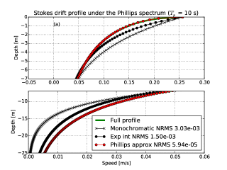
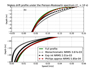
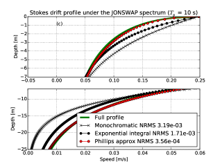
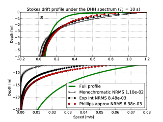
The assumption that the Phillips profile is a good fit to parametric spectra can also be tested in a more straightforward manner without making any assumption of the behaviour of the quantity by simply fitting a Phillips profile () to various spectra. In Fig 1 we have fitted the Phillips profile to the surface Stokes drift and the transport from parametric spectra and compared the approximate profile to the full profile. The results show that for the Phillips spectrum the approximation matches the full profile (to within roundoff error). More interestingly, the Pierson-Moskowitz and the JONSWAP spectra are both very well represented by the Phillips approximation (see Fig 1). This simply confirms what we found in Table 1. A more challenging case is the Donelan-Hamilton-Hui (DHH) spectrum (Donelan et al., 1985) which has an tail,
| (28) |
and will consequently behave very differently in the tail. The spectrum is identical to the JONSWAP spectrum except for substitution of the peak frequency for and a Jacobian transformation removing the factor in the exponential. It is worth noting that the surface Stokes drift under the DHH spectrum is ill-defined (Webb and Fox-Kemper, 2011, 2015), since
| (29) |
which is unbounded because the integrand asymptotes to
| (30) |
Setting a cut-off frequency at yields the results shown in Fig 1 for s. As can be seen the Phillips approximation is not good, but it does in fact represent a small improvement compared with the monochromatic and exponential integral approximations.
4 ERA-Interim spectra in open-ocean conditions
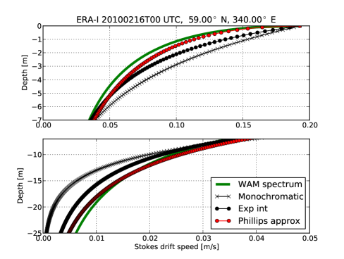
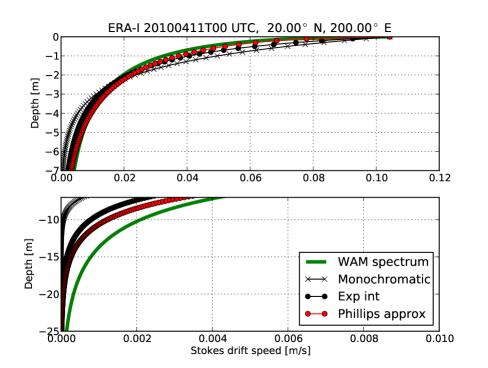
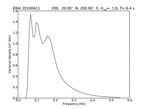
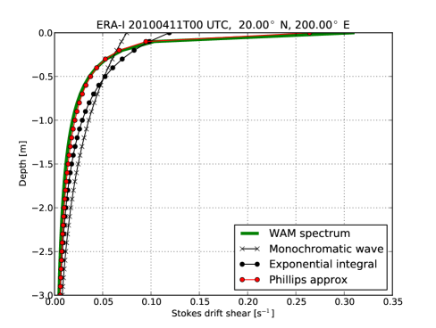
Although can be estimated from the spectrum as shown in Eq (21), it is a quantity which will not be generally available from wave models. We find that is a very good approximation for a dataset of two-dimensional spectra taken from the ERA-Interim reanalysis (Dee et al., 2011) in the North Atlantic Ocean for the period of 2010 (same location as used by BJB) as well as a swell-dominated location near Hawaii (N, W). The temporal resolution is six hours and the spatial resolution of the wave model component of ERA-Interim is approximately 110 km. The angular resolution is while the frequency resolution is logarithmic over 30 frequency bins from Hz. We have computed the two-dimensional Stokes drift velocity vector at every 10 cm from the surface down to 30 m depth from the full spectra. Comparing the approximate profiles to the full profiles (see Figs 2-3) reveals that in most cases the Phillips profile (19) is a closer match to the full profile than the exponential integral profile (7), even in cases with very complex spectra (see the tri-peaked spectrum in Fig 4 associated with the profile in Fig 3b). In particular, it is a very good match to the shear near the surface, which becomes very high, and in the case of the Phillips spectrum infinite. Fig 5 reveals the much stronger shear near the surface achieved by the Phillips profile. In fact, the gradient is an almost perfect match to that of the full profile. This is unsurprising since near the surface the high-frequency tail will dominate the shear. ECWAM adds a high-frequency diagnostic tail (ECMWF, 2013)
| (31) |
where . This integral is similar to (10) and the solution is similar to (19) [see eg Gradshteyn and Ryzhik 2007, Eq (3.461.5)], yielding
| (32) |
For the surface Stokes drift this simplifies to
| (33) |
Here, the cut-off frequency of ECWAM is related to the mean wind sea frequency as . Eq (31) is exactly the profile under the Phillips spectrum (9) on which our approximation is based and it is unsurprising then that the profile (11) is a good match to the full profile as we get close to the surface where the high frequency part of the spectrum dominates the Stokes drift velocity.
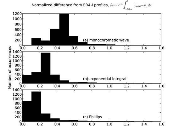
Fig 6 shows that the Phillips profile has an NRMS deviation about half that of the exponential integral profile for the North Atlantic location. The numbers are quite similar for the Hawaii swell location.
5 Discussion and concluding remarks
Although the exponential integral profile proposed by BJB represents a major improvement over the monochromatic profile, it appears clear that the Phillips profile (10) is a much better match, especially for representing the shear near the surface; see Eq (15). Studies of ERA-Interim spectra at two open-ocean locations near Hawaii and in the North Atlantic Ocean show that is a very good estimate for a wide range of sea states. This allows us to compute the profile from the same two parameters as the monochromatic profile, namely the transport and the surface Stokes drift velocity, and it is thus no more expensive to employ in ocean modelling. We have shown here that the profile works remarkably well in a variety of situations, including swell-dominated cases. In C it is shown that the profile is also a better match for profiles under measured 2 Hz spectra in the central North Sea. This shows that the fit is not dependent on the assumption of an tail since these spectra have no high-frequency diagnostic tail added to them. The new profile also comes closer to the DHH spectrum which has an tail, but here the match is naturally quite poor (see Fig 1). We conclude that for applications concerned with the shear of the profile, in particular studies of Langmuir turbulence, the proposed profile is a much better choice than the monochromatic profile, but it is also clearly a better option than the previously proposed exponential integral profile.
The question of how best to represent a full two-dimensional Stokes drift velocity profile with a one-dimensional profile was discussed by BJB where it was argued that using the mean wave direction is better than using the surface Stokes drift direction since the latter would be heavily weighted toward the direction of high-frequency waves. This still holds true, but it is clear that spreading due to multi-directional waves affects the Stokes drift [see Webb and Fox-Kemper 2015], and although we model the average profile well, situations with for example opposing swell and wind waves will greatly modify individual profiles. This will also affect the Langmuir turbulence as parameterised from the Stokes drift velocity profile, as demonstrated by McWilliams et al. (2014) for an idealised case of swell and wind waves propagating in different directions. Li et al. (2015) investigated the impact of wind-wave misalignment and Stokes drift penetration depth on upper ocean mixing Southern Ocean warm bias with a coupled wave-atmosphere-ocean earth system model and found that Langmuir turbulence, parameterized using a -profile parameterization (Large et al., 1994). They found a substantial reduction in the demonstrated that a K-profile parameterization for a coupled system consisting of a spectral wave model and the Community Earth System Model. This is impossible to model with a simple parametric profile like the one proposed here, but a combination of two such parametric profiles, one for the swell and one representing the wind waves is straightforward to implement.
The method presented here to derive an approximate Stokes drift profile based on the Phillips profile could also be relevant for other wave-related processes. The proposed mixing by non-breaking waves (Babanin, 2006) was implemented in a climate model of intermediate complexity by Babanin et al. (2009) and was compared against tank measurements by Babanin and Haus (2009). In a similar vein, mixing induced by the wave orbital motion as suggested by Qiao et al. (2004) has been tested for ocean general circulation models (Qiao et al., 2010; Huang et al., 2011; Fan and Griffies, 2014). These suggested mixing parameterizations bear some semblance to the Langmuir turbulence parameterization in that they involve the shear of an integral of the wave spectrum with an exponential decay term. Qiao et al. (2004) proposes to enhance the diffusion coefficient by adding a term which involves the second moment of the wave spectrum. It will thus be somewhat less sensitive to the higher frequencies than the Stokes drift velocity profile. By again assuming that the wave spectrum is represented by the Phillips spectrum (9), we find an analytical expression for the mixing coefficient (see B). Although we do not pursue this any further here it is worth noting that similar approximations to those presented for the Stokes drift profile could thus be found for the proposed wave-induced mixing by Qiao et al. (2004).
Wave-induced processes in the ocean surface mixed layer have long been considered important for modelling the mixing and the currents in the upper part of the ocean. Using the proposed profile for the Stokes drift velocity profile is a step towards efficiently parameterising these processes. Although more work is needed to quantify the impact of these processes on ocean-only and coupled models, it appears clear that the impact on the sea surface temperature (SST) may be on the order of 0.5 K (Fan and Griffies, 2014; Janssen et al., 2013; Breivik et al., 2015). As the coupled atmosphere-ocean system is sensitive to such biases, for instance through the triggering of atmospheric deep convection, see Sheldon and Czaja (2014), wave-induced mixing could play an important role in improving the performance of coupled climate and forecast models.
Acknowledgment
This work has been carried out with support from the European Union FP7 project MyWave (grant no 284455). Thanks to the three anonymous reviewers and editor Will Perrie for detailed and constructive comments that greatly improved the manuscript.
| Spectral shape | NRMS Phillips | NRMS exp int | |
|---|---|---|---|
| Phillips | 1 | 0.001 | 0.573 |
| JONSWAP () | 0.96 | 0.148 | 0.650 |
| PM | 1.05 | 0.231 | 0.957 |
| JONSWAP+swell ( Hz) | 0.94 | 0.058 | 0.581 |
| PM+l.f. swell ( Hz) | 1.04 | 0.240 | 0.920 |
 |
 |
 |
 |
Appendix A The transport under a Phillips-type spectrum
The Stokes transport under Eq (19) is
| (34) |
The second term can be solved by applying Eq (6.281.1) of Gradshteyn and Ryzhik 2007 as follows. Introduce the variable substitution and rewrite the second term (marked GR6.281.1) in Eq (34)
| (35) |
We can now introduce and and employ Eq (6.281.1) of Gradshteyn and Ryzhik 2007,
| (36) |
The full integral (34) can now be written
| (37) |
Appendix B An analytical expression for the wave-induced mixing coefficient of Qiao et al. (2004)
The wave-induced mixing coefficient proposed by Qiao et al. (2004) can be written
| (38) |
where the mixing length is assumed proportional to the wave orbital radius. We assume that the wave spectrum is represented by the Phillips frequency spectrum (9), which renders the integral in Eq (38) as
| (39) |
After integration by parts and by performing a variable substitution a solution to the integral (39) can be found from Eq (3.352.2) of Gradshteyn and Ryzhik (2007),
| (40) |
Appendix C A comparison against measured spectra in the central North Sea
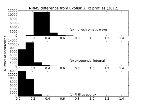
We have estimated the profile from the same observational spectra as was used by BJB from the Ekofisk location in the central North Sea for the period 2012 (more than 24,000 spectra in total). The location is (N, E). The sampling rate was 2 Hz and 20-minute spectra were computed as described by BJB. The NRMS difference is shown in Fig C.1. As can be seen from Panel c, the new profile reduces the NRMS difference slightly compared with the exponential integral and quite dramatically compared with the monochromatic profile. It is worth noting that no tail has been fitted to the spectra, so the improvement is present even without adding a high-frequency tail.
References
- Ardhuin and Jenkins (2006) Ardhuin, F. and A. Jenkins, 2006: On the Interaction of Surface Waves and Upper Ocean Turbulence. J Phys Oceanogr, 36, 551–557, doi:10.1175/2009JPO2862.1.
- Ardhuin et al. (2009) Ardhuin, F., L. Marié, N. Rascle, P. Forget, and A. Roland, 2009: Observation and estimation of Lagrangian, Stokes and Eulerian currents induced by wind and waves at the sea surface. J Phys Oceanogr, 39, 2820–2838, doi:10.1175/2009JPO4169.1.
- Axell (2002) Axell, L. B., 2002: Wind-driven internal waves and Langmuir circulations in a numerical ocean model of the southern Baltic Sea. J Geophys Res, 107 (C11), 20, doi:10.1029/2001JC000922.
- Babanin (2006) Babanin, A. V., 2006: On a wave-induced turbulence and a wave-mixed upper ocean layer. Geophys Res Lett, 33 (20), 6, doi:10.1029/2006GL027308.
- Babanin et al. (2009) Babanin, A. V., A. Ganopolski, and W. R. Phillips, 2009: Wave-induced upper-ocean mixing in a climate model of intermediate complexity. Ocean Model, 29 (3), 189–197, doi:10.1016/j.ocemod.2009.04.003.
- Babanin and Haus (2009) Babanin, A. V. and B. K. Haus, 2009: On the existence of water turbulence induced by nonbreaking surface waves. J Phys Oceanogr, 39 (10), 2675–2679, doi:10.1175/2009JPO4202.1.
- Belcher et al. (2012) Belcher, S. E., et al., 2012: A global perspective on Langmuir turbulence in the ocean surface boundary layer. Geophys Res Lett, 39 (18), 9, doi:10.1029/2012GL052932.
- Breivik et al. (2013) Breivik, Ø., A. Allen, C. Maisondieu, and M. Olagnon, 2013: Advances in Search and Rescue at Sea. Ocean Dyn, 63 (1), 83–88, arXiv:1211.0805, doi:10/jtx.
- Breivik et al. (2012) Breivik, Ø., A. Allen, C. Maisondieu, J.-C. Roth, and B. Forest, 2012: The Leeway of Shipping Containers at Different Immersion Levels. Ocean Dyn, 62 (5), 741–752, arXiv:1201.0603, doi:10.1007/s10236-012-0522-z, sAR special issue.
- Breivik et al. (2014) Breivik, Ø., P. Janssen, and J. Bidlot, 2014: Approximate Stokes Drift Profiles in Deep Water. J Phys Oceanogr, 44 (9), 2433–2445, arXiv:1406.5039, doi:10.1175/JPO-D-14-0020.1.
- Breivik et al. (2015) Breivik, Ø., K. Mogensen, J.-R. Bidlot, M. A. Balmaseda, and P. A. Janssen, 2015: Surface Wave Effects in the NEMO Ocean Model: Forced and Coupled Experiments. J Geophys Res Oceans, 120, arXiv:1503.07 677, doi:10.1002/2014JC010565.
- Carniel et al. (2005) Carniel, S., M. Sclavo, L. H. Kantha, and C. A. Clayson, 2005: Langmuir cells and mixing in the upper ocean. Il Nuovo Cimento C Geophysics Space Physics C, 28C, 33–54, doi:10.1393/ncc/i2005-10022-8.
- Carrasco et al. (2014) Carrasco, A., A. Semedo, P. E. Isachsen, K. H. Christensen, and Ø. Saetra, 2014: Global surface wave drift climate from ERA-40: the contributions from wind-sea and swell. Ocean Dyn, 64 (12), 1815–1829, doi:10.1007/s10236-014-0783-9, 13th wave special issue.
- Craik (1977) Craik, A., 1977: The generation of Langmuir circulations by an instability mechanism. J Fluid Mech, 81, 209–223, doi:10.1017/S0022112077001980.
- Craik and Leibovich (1976) Craik, A. and S. Leibovich, 1976: A rational model for Langmuir circulations. J Fluid Mech, 73 (03), 401–426, doi:10.1017/S0022112076001420.
- Dee et al. (2011) Dee, D., et al., 2011: The ERA-Interim reanalysis: Configuration and performance of the data assimilation system. Q J R Meteorol Soc, 137 (656), 553–597, doi:10.1002/qj.828.
- Donelan et al. (1985) Donelan, M. A., J. Hamilton, and W. H. Hui, 1985: Directional spectra of wind-generated waves. Phil Trans R Soc Lond A, 315, 509–562, doi:10.1098/rsta.1985.0054.
- ECMWF (2013) ECMWF, 2013: IFS Documentation CY40r1, Part VII: ECMWF Wave Model. ECMWF Model Documentation, European Centre for Medium-Range Weather Forecasts, 79 pp, available at http://old.ecmwf.int/research/ifsdocs/CY40r1/ pp.
- Faller and Caponi (1978) Faller, A. J. and E. A. Caponi, 1978: Laboratory studies of wind-driven Langmuir circulations. J Geophys Res, 83 (C7), 3617–3633, doi:10.1029/JC083iC07p03617.
- Fan and Griffies (2014) Fan, Y. and S. M. Griffies, 2014: Impacts of parameterized Langmuir turbulence and non-breaking wave mixing in global climate simulations. J Climate, doi:10.1175/JCLI-D-13-00583.1.
- Flór et al. (2010) Flór, J. B., E. J. Hopfinger, and E. Guyez, 2010: Contribution of coherent vortices such as Langmuir cells to wind-driven surface layer mixing. J Geophys Res Oceans, 115 (C10), doi:10.1029/2009JC005900, c10031.
- Gradshteyn and Ryzhik (2007) Gradshteyn, I. and I. Ryzhik, 2007: Table of Integrals, Series, and Products, 7th edition. Edited by A. Jeffrey and D. Zwillinger, Academic Press, London, 1221 pp.
- Grant and Belcher (2009) Grant, A. L. and S. E. Belcher, 2009: Characteristics of Langmuir turbulence in the ocean mixed layer. J Phys Oceanogr, 39 (8), 1871–1887, doi:10.1175/2009JPO4119.1.
- Hasselmann (1970) Hasselmann, K., 1970: Wave-driven inertial oscillations. Geophys Astrophys Fluid Dyn, 1 (3-4), 463–502, doi:10.1080/03091927009365783.
- Hasselmann et al. (1973) Hasselmann, K., et al., 1973: Measurements of wind-wave growth and swell decay during the Joint North Sea Wave Project (jonswap). Deutsch Hydrogr Z, A8 (12), 1–95.
- Huang et al. (2011) Huang, C. J., F. Qiao, Z. Song, and T. Ezer, 2011: Improving simulations of the upper ocean by inclusion of surface waves in the Mellor-Yamada turbulence scheme. J Geophys Res, 116 (C1), doi:10.1029/2010JC006320.
- Janssen (2012) Janssen, P., 2012: Ocean Wave Effects on the Daily Cycle in SST. J Geophys Res Oceans, 117, 24, doi:10/mth.
- Janssen et al. (2004) Janssen, P., O. Saetra, C. Wettre, H. Hersbach, and J. Bidlot, 2004: Impact of the sea state on the atmosphere and ocean. Annales hydrographiques, Service hydrographique et océanographique de la marine, Vol. 3-772, 3.1–3.23.
- Janssen et al. (2013) Janssen, P., et al., 2013: Air-Sea Interaction and Surface Waves. ECMWF Technical Memorandum 712, European Centre for Medium-Range Weather Forecasts, 36 pp.
- Jenkins (1987) Jenkins, A. D., 1987: Wind and wave induced currents in a rotating sea with depth-varying eddy viscosity. J Phys Oceanogr, 17, 938–951, doi:10/fdwvq2.
- Kantha and Clayson (2000) Kantha, L. H. and C. A. Clayson, 2000: Small scale processes in geophysical fluid flows, Vol. 67. Academic Press.
- Kantha and Clayson (2004) Kantha, L. H. and C. A. Clayson, 2004: On the effect of surface gravity waves on mixing in the oceanic mixed layer. Ocean Model, 6 (2), 101–124, doi:10.1016/S1463-5003(02)00062-8.
- Kenyon (1969) Kenyon, K. E., 1969: Stokes Drift for Random Gravity Waves. J Geophys Res, 74 (28), 6991–6994, doi:10.1029/JC074i028p06991.
- Langmuir (1938) Langmuir, I., 1938: Surface motion of water induced by wind. Science, 87 (2250), 119–123, doi:10.1126/science.87.2250.119.
- Large et al. (1994) Large, W. G., J. C. McWilliams, and S. C. Doney, 1994: Oceanic vertical mixing: A review and a model with a nonlocal boundary layer parameterization. Rev Geophys, 32 (4), 363–403, doi:10.1029/94RG01872.
- Leibovich (1977) Leibovich, S., 1977: Convective instability of stably stratified water in the ocean. J Fluid Mech, 82, 561–581, doi:10.1017/S0022112077000846.
- Leibovich (1980) Leibovich, S., 1980: On wave-current interaction theories of Langmuir circulations. J Fluid Mech, 99, 715–724, doi:10.1017/S0022112080000857.
- Leibovich (1983) Leibovich, S., 1983: The form and dynamics of Langmuir circulations. Annu Rev Fluid Mech, 15 (1), 391–427, doi:10.1146/annurev.fl.15.010183.002135.
- Li and Garrett (1997) Li, M. and C. Garrett, 1997: Mixed layer deepening due to Langmuir circulation. J Phys Oceanogr, 27 (1), 121–132, doi:10/cmhvrr.
- Li et al. (2015) Li, Q., A. Webb, B. Fox-Kemper, A. Craig, G. Danabasoglu, W. G. Large, and M. Vertenstein, 2015: Langmuir mixing effects on global climate: WAVEWATCH III in CESM. Ocean Model, doi:10.1016/j.ocemod.2015.07.020.
- McWilliams et al. (1997) McWilliams, J., P. Sullivan, and C.-H. Moeng, 1997: Langmuir turbulence in the ocean. J Fluid Mech, 334 (1), 1–30, doi:10.1017/S0022112096004375.
- McWilliams et al. (2014) McWilliams, J. C., E. Huckle, J. Liang, and P. Sullivan, 2014: Langmuir turbulence in swell. J Phys Oceanogr, 44, 870–890, doi:10.1175/JPO-D-13-0122.1.
- McWilliams and Restrepo (1999) McWilliams, J. C. and J. M. Restrepo, 1999: The Wave-driven Ocean Circulation. J Phys Oceanogr, 29 (10), 2523–2540, doi:10/dwj9tj.
- McWilliams and Sullivan (2000) McWilliams, J. C. and P. P. Sullivan, 2000: Vertical mixing by Langmuir circulations. Spill Science and Technology Bulletin, 6 (3), 225–237, doi:10.1016/S1353-2561(01)00041-X.
- Phillips (1958) Phillips, O. M., 1958: The equilibrium range in the spectrum of wind-generated waves. J Fluid Mech, 4, 426–434, doi:10.1017/S0022112058000550.
- Pierson and Moskowitz (1964) Pierson, W. J., Jr and L. Moskowitz, 1964: A proposed spectral form for fully developed wind seas based on the similarity theory of S A Kitaigorodskii. J Geophys Res, 69, 5181–5190.
- Polton et al. (2005) Polton, J. A., D. M. Lewis, and S. E. Belcher, 2005: The role of wave-induced Coriolis-Stokes forcing on the wind-driven mixed layer. J Phys Oceanogr, 35 (4), 444–457, doi:10.1175/JPO2701.1.
- Qiao et al. (2010) Qiao, F., Y. Yuan, T. Ezer, C. Xia, Y. Yang, X. Lü, and Z. Song, 2010: A three-dimensional surface wave–ocean circulation coupled model and its initial testing. Ocean Dyn, 60 (5), 1339–1355, doi:10.1007/s10236-010-0326-y.
- Qiao et al. (2004) Qiao, F., Y. Yuan, Y. Yang, Q. Zheng, C. Xia, and J. Ma, 2004: Wave-induced mixing in the upper ocean: Distribution and application to a global ocean circulation model. Geophys Res Lett, 31 (11), 4, doi:10.1029/2004GL019824.
- Rascle and Ardhuin (2013) Rascle, N. and F. Ardhuin, 2013: A global wave parameter database for geophysical applications. Part 2: Model validation with improved source term parameterization. Ocean Model, 70, 174–188, doi:10.1016/j.ocemod.2012.12.001.
- Rascle et al. (2008) Rascle, N., F. Ardhuin, P. Queffeulou, and D. Croize-Fillon, 2008: A global wave parameter database for geophysical applications. Part 1: Wave-current-turbulence interaction parameters for the open ocean based on traditional parameterizations. Ocean Model, 25 (3–4), 154–171, doi:10.1016/j.ocemod.2008.07.006.
- Rascle et al. (2006) Rascle, N., F. Ardhuin, and E. Terray, 2006: Drift and mixing under the ocean surface: A coherent one-dimensional description with application to unstratified conditions. J Geophys Res, 111 (C3), 16, doi:10.1029/2005JC003004.
- Reistad et al. (2011) Reistad, M., Ø. Breivik, H. Haakenstad, O. J. Aarnes, B. R. Furevik, and J.-R. Bidlot, 2011: A high-resolution hindcast of wind and waves for the North Sea, the Norwegian Sea, and the Barents Sea. J Geophys Res Oceans, 116, 18 pp, C05 019, arXiv:1111.0770, doi:10/fmnr2m.
- Röhrs et al. (2012) Röhrs, J., K. Christensen, L. Hole, G. Broström, M. Drivdal, and S. Sundby, 2012: Observation-based evaluation of surface wave effects on currents and trajectory forecasts. Ocean Dyn, 62 (10–12), 1519–1533, doi:10.1007/s10236-012-0576-y, sAR special issue.
- Röhrs et al. (2015) Röhrs, J., A. Sperrevik, K. Christensen, Ø. Breivik, and G. Broström, 2015: Comparison of HF radar measurements with Eulerian and Lagrangian surface currents. Ocean Dyn, 1–12, doi:10.1007/s10236-015-0828-8.
- Saetra et al. (2007) Saetra, Ø., J. Albretsen, and P. Janssen, 2007: Sea-State-Dependent Momentum Fluxes for Ocean Modeling. J Phys Oceanogr, 37 (11), 2714–2725, doi:10.1175/2007JPO3582.1.
- Semedo et al. (2015) Semedo, A., R. Vettor, Ø. Breivik, A. Sterl, M. Reistad, C. G. Soares, and D. C. A. Lima, 2015: The Wind Sea and Swell Waves Climate in the Nordic Seas. Ocean Dyn, 65 (2), 223–240, doi:10.1007/s10236-014-0788-4, 13th wave special issue.
- Sheldon and Czaja (2014) Sheldon, L. and A. Czaja, 2014: Seasonal and interannual variability of an index of deep atmospheric convection over western boundary currents. Q J R Meteorol Soc, 140 (678), 22–30, doi:10.1002/qj.2103.
- Skyllingstad and Denbo (1995) Skyllingstad, E. D. and D. W. Denbo, 1995: An ocean large-eddy simulation of Langmuir circulations and convection in the surface mixed layer. J Geophys Res, 100 (C5), 8501–8522, doi:10.1029/94JC03202.
- Stokes (1847) Stokes, G. G., 1847: On the theory of oscillatory waves. Trans Cambridge Philos Soc, 8, 441–455.
- Stull (1988) Stull, R. B., 1988: An introduction to boundary layer meteorology. Kluwer, New York, 666 pp.
- Tamura et al. (2012) Tamura, H., Y. Miyazawa, and L.-Y. Oey, 2012: The Stokes drift and wave induced-mass flux in the North Pacific. J Geophys Res, 117 (C8), 14, doi:10.1029/2012JC008113.
- Thorpe (2004) Thorpe, S., 2004: Langmuir Circulation. Annu Rev Fluid Mech, 36, 55–79, doi:10.1146/annurev.fluid.36.052203.071431.
- Webb and Fox-Kemper (2011) Webb, A. and B. Fox-Kemper, 2011: Wave spectral moments and Stokes drift estimation. Ocean Model, 40, 273–288, doi:10.1016/j.ocemod.2011.08.007.
- Webb and Fox-Kemper (2015) Webb, A. and B. Fox-Kemper, 2015: Impacts of wave spreading and multidirectional waves on estimating Stokes drift. Ocean Model, 16, doi:10.1016/j.ocemod.2014.12.007.
- Weber (1983) Weber, J. E., 1983: Steady Wind- and Wave-Induced Currents in the Open Ocean. J Phys Oceanogr, 13, 524–530, doi:10/djz6md.