IDCS J1426.5+3508: Weak Lensing Analysis of a Massive Galaxy Cluster at
Abstract
We present a weak lensing study of the galaxy cluster IDCS J1426.5+3508 at , which is the highest redshift strong lensing cluster known and the most distant cluster for which a weak lensing analysis has been undertaken. Using F160W, F814W, and F606W observations with the Hubble Space Telescope, we detect tangential shear at significance. Fitting a Navarro-Frenk-White mass profile to the shear with a theoretical median mass-concentration relation, we derive a mass M⊙. This mass is consistent with previous mass estimates from the Sunyaev-Zel’dovich (SZ) effect, X-ray, and strong lensing. The cluster lies on the local SZ-weak lensing mass scaling relation observed at low redshift, indicative of minimal evolution in this relation.
Subject headings:
cosmology: observations – dark matter – galaxies: clusters: individual (IDCS J1426.5+3508) – gravitational lensing: weak.1. Introduction
Massive, high-redshift galaxy clusters, though rare, provide valuable information about cosmological parameters, structure formation, and galaxy evolution. The redshift regime represents a critical era during which significant star formation occurs in cluster galaxies (e.g, Tran et al., 2010; Brodwin et al., 2013; Bayliss et al., 2014; Webb et al., 2015b; Alberts et al., 2014). Only a handful of clusters at redshift have been confirmed to date (e.g, Newman et al., 2014; Papovich et al., 2010; Zeimann et al., 2012; Muzzin et al., 2013; Tozzi et al., 2015; Webb et al., 2015a), thanks in part to large X-ray, infrared, and Sunyaev-Zel’dovich (SZ) effect surveys (e.g., Eisenhardt et al., 2008; Fassbender et al., 2011; Wylezalek et al., 2014; Bleem et al., 2015).
In this paper we focus upon the galaxy cluster IDCS J1426.5+3508. This cluster was first discovered in the IRAC Distant Cluster Survey (IDCS). Follow-up with the Hubble Space Telescope (HST) Wide Field Camera-3 (WFC3) grism and the Low Resolution Imaging Spectrometer (LRIS, Oke et al., 1995) on the W. M. Keck Observatory spectroscopically confirms a redshift of (Stanford et al., 2012). With ks of Chandra data, Brodwin et al. (2015) obtain mass estimates based upon the X-ray temperature, gas mass, and the product of core-excised X-ray temperature and gas mass of M⊙, M⊙, and M⊙, respectively. In comparison, SZ observations with the Combined Array for Research in Millimeter-wave Astronomy (CARMA) indicate M⊙ (Brodwin et al., 2012), implying M⊙ with a Duffy et al. (2008) mass-concentration relation. These mass estimates establish IDCS J1426.5+3508 as the most massive galaxy cluster confirmed at redshift . For comparison, another high-redshift cluster, XDCP J0044.0-2033 (), has mass derived from the Vikhlinin et al. (2009) M scaling relation M⊙ (Tozzi et al., 2015).
Moreover, IDCS J1426.5+3508 is also the most distant strong lensing galaxy cluster. A giant gravitationally lensed arc associated with the cluster was discovered in HST/WFC3 and Advanced Camera for Surveys (ACS) imaging. An initial redshift estimate based on broadband photometry yielded for the arc and a lower limit of M⊙ for the cluster via a strong-lensing analysis (Gonzalez et al., 2012). For CDM, Gonzalez et al. (2012) calculate that the expected number of giant arcs at this redshift and brightness is vanishingly small, highlighting the long-standing arc statistics problem (see Meneghetti et al., 2013, for a recent review). One explanation suggested to explain the observed arc in IDCS J1426.5+3508 is that the cluster might have a substantially more concentrated density profile—and hence an enhanced lensing cross-section—than predicted for a cluster at this epoch.
Gravitational weak lensing determines the cluster mass via the distortion in shape of background galaxies due to the gravitational potential of the cluster. Unlike mass estimates derived from X-ray or SZ observations, weak lensing measures the mass distribution independent of the dynamical state or hydrostatic equilibrium of the cluster. Thus, weak lensing is also a powerful tool for calibrating X-ray or SZ mass estimates (e.g., Marrone et al., 2012; Hoekstra et al., 2012; Jee et al., 2011). Furthermore, the mass and concentration of the cluster can in principle be determined without a prescribed mass-concentration relationship.
However, weak lensing is observationally challenging, particularly for distant clusters. Because the lensing cluster is at high redshift, the number of lensed background galaxies is small, decreasing the lensing signal. Also, the extent of the distortions to be measured is on the scale of the observational point spread function (PSF; e.g., Rhodes et al., 2007; Jee et al., 2007). Deep, space-based observations with well-understood PSFs are therefore required to obtain high fidelity measurements of the weak lensing distortion.
In this work, we demonstrate the feasibility of weak lensing analyses at . IDCS J1426.5+3508 is the highest redshift cluster to have joint X-ray, SZ, and weak lensing observations, and thus provides an opportunity to compare whether the scaling relations between these mass estimators, derived at low redshift, remain valid at this epoch. In Section 2 we describe the observations and data analysis, including the selection of source galaxies. We outline the measurement of galaxy shapes and the correction for PSF distortion in those measurements in Section 3. The weak lensing shear profile is presented in Section 4. We discuss the mass estimation and SZ-weak lensing scaling relation in Sections 5 and 6, respectively, and summarize our findings in Section 7.
Throughout the paper, we adopt the nine-year Wilkinson Microwave Anisotropy Probe (WMAP9) cosmological parameters of , , and km s-1 Mpc-1 (Hinshaw et al., 2013) and define . All magnitudes are in the AB system (Oke & Gunn, 1983). We take the F606W image for our shape measurement and the center of the cluster to be the location of the brightest cluster galaxy (BCG), as identified by Stanford et al. (2012). Unless otherwise stated, we report masses as overdensities relative to the critical density.
2. Observations
For our analysis, we use HST data from Cycle 20 taken on 2012 December 19, and 2013 April 17-19, with the ACS F606W (V-band), F814W (I-band), and WFC3 F160W (H-band) filters for a total of 21760, 8108, and 4947 seconds, respectively. We also use Cycle 17 observations from 2010 July 8 and 2010 November 7 with the F814W and F160W filters for 4513 and 2612 seconds, respectively. Since the F160W data are mosaicked, the effective exposure time for the central region is 7559 seconds while the minimum exposure time for the outer regions is 1212 seconds. The cluster is also among the targets in HST GO-program 13677 (PI Perlmutter) which will add observations in WFC3 F140W, F105W, and F814W filters for future studies of this cluster.
2.1. HST ACS Data Reduction
We performed basic processing of the ACS data with the CALACS pipeline. Our only modification to the standard procedure was to employ the charge transfer inefficiency (CTI) correction method developed by Massey et al. (2010, 2014) to correct for CTI degradation prior to running CALACS. CTI extends the shapes of galaxies and, if uncorrected, can imitate the effects of weak lensing. Astrometric shifts, geometric distortion correction, sky subtraction, cosmic ray removal, and final image stacking were handled by the standard TweakReg and Astrodrizzle packages. Images were drizzled to a pixel scale with a Gaussian kernel and pixel fraction of 1.0. Rhodes et al. (2007) showed that changing the pixel scale from the ACS native scale of to optimizes our ability to correct for PSF effects while the results are largely insensitive to the choice of pixel fraction.
2.2. Source Galaxy Catalog
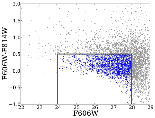
Starting with F606W as our detection image, we extracted a catalog of 4771 sources with SExtractor (Bertin & Arnouts, 1996) with a criteria of connecting pixels brighter than a sky rms of . We then obtained matched photometry for these sources in F814W and F160W by running SExtractor in dual image mode. Figure 1 is the resulting color-magnitude diagram for the two bluest filters.
We identify the foreground and cluster galaxy contamination in our catalog via color selection. One benefit of employing an F606W-selected catalog is that most cluster red sequence galaxies are non-detections. Listed below are the sequence of color and size cuts applied to distinguish among foreground galaxies, cluster members, and background galaxies. We detect 3050 objects with F606W, the approximate depth of our observations. We first reject sources with either F606W or FWHM to exclude bright and large objects that are probable foreground galaxies. Based on a Bruzual & Charlot (2003) model of a star-forming galaxy with , we next implement a color cut of F606W-F814W to eliminate additional foreground galaxies in our sample. To reject cluster members on the red sequence, we rule out objects with F814W-F160W (Stanford et al., 2012). We also cut objects with signal to noise .
In addition, we exclude objects based on shape measurements constraints, further discussed in Section 3. The final catalog for the shear analysis consists of 1011 sources, equivalent to arcmin-2. As a cross-check, we construct a radial density profile for the remaining galaxies centered on the BCG. There is no central excess evident in the radial profile, indicating that residual contamination from blue cluster galaxies is minimal.
2.3. Redshift Distribution
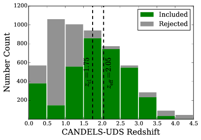
Given the redshift of the cluster, compiling a clean catalog of background sources is not possible with the available photometric data. However, we can control the foreground contamination in our source catalog statistically. We estimate the redshift distribution of our source catalog using the Cosmic Assembly Near-infrared Deep Extragalactic Legacy Survey Ultra Deep Survey (CANDELS-UDS) multiwavelength catalog (Santini et al., 2014) which provides infrared-detected sources to an F160W magnitude limit of in a range of filters. Employing the selection criteria described in Section 2.2, we found 3512 sources, 46% of which were contaminants with . The distribution of CANDELS-UDS redshift for sources included and excluded by our selection criteria is illustrated in Figure 2.
We estimate the effective redshift of the source population by calculating the lensing efficiency, the mean of the ratio of angular diameter distances,
| (1) |
where and are the angular diameter distances between the lens and the source and the observer and the source, respectively. We set a floor of to account for foreground sources with . For the subset of CANDELS-UDS sources matching our selection criteria, we compute , corresponding to an effective redshift , and width .
Despite CANDELS-UDS being the deepest catalog with data in our set of filters, 12% of the galaxies in our background source catalog are fainter in F160W than the CANDELS-UDS limiting magnitude. To investigate the effects of the mismatch in detection filter threshold between our data and the CANDELS-UDS catalog, we randomly select 114 objects from a sample of CANDELS-UDS objects near the survey limiting magnitude () and add their redshifts to the 3512 CANDELS-UDS sources matching our selection criteria. We choose these objects because they are most likely to mimic the redshift distribution of the sources with F160W missing from the CANDELS-UDS catalog. We then repeat our calculation of using Equation 1 with the additional 12% of galaxies. Including the randomly selected redshift sample increases by . This source of uncertainty for is a subdominant contributor to the total mass error budget.
3. Shape Measurement
3.1. RRG Method
We measure galaxy distortions by applying the RRG method developed by Rhodes et al. (2000), which calculates the second- and fourth-order Gaussian-weighted moments of each galaxy to determine ellipticity and correct for convolutions with the PSF. The weak lensing shear is then derived from the average ellipticity of the sources. We choose the weight function size of each object to be where and are the semi-major and -minor axes in pixels calculated from SExtractor.
For each object, the shear is related to the ellipticity of that object
| (2) |
where is the shear susceptibility calculated from our data and is a calibration factor determined from the analysis of simulated images containing a known shear (Leauthaud et al., 2007). The reduced shear is then
| (3) |
where is the convergence. We further incorporate the width of the redshift distribution (Seitz & Schneider, 1997). The observed shear is then
| (4) |
In addition to the criteria presented in Section 2.2, we introduce more selection criteria to our background source catalog due to shape measurement limitations. The RRG method cannot correct for the distortion on objects smaller than times the RRG weight function width of . Therefore, we reject galaxies with a SExtractor FWHM for which we were not able to apply a PSF correction. Also, we exclude objects that encountered centroiding errors during shape measurement or for which the PSF correction did not converge. Therefore, our final catalog for weak lensing analysis includes 1011 sources.
3.2. PSF Correction
The ACS PSF is known to be both temporally and spatially variable. Thermal breathing of the telescope, dependent on the 90-minute orbit of HST, and a slow deviation in the focus on the timescale of a few weeks further complicate the PSF. In the weak lensing regime, an uncorrected PSF distortion can drown out the signal, so precise characterization is critical.
We use the publicly available TinyTim software111http://tinytim.stsci.edu/ (Krist & Hook, 1997; Krist et al., 2011) to theoretically model the PSF distortion across our image. TinyTim simulates the PSF given a focus value and takes into account the instrument, chip number, chip position, filter, and spectrum of the object. Schrabback et al. (2010) notes additional variations in the PSF dependent on relative sun angle, but finds that of variations can be described solely by the focus parameter.
Our F606W image is a combination of 16 separate frames. We replicate the PSF in each frame individually by specifying a focus value determined by the HST focus model222http://focustool.stsci.edu/, applying the average focus during the exposure period of each individual frame. Adopting a modified version of TinyTim333http://community.dur.ac.uk/r.j.massey/acs/PSF, we generate a distortion-corrected grid of PSFs across the entire image with pixel scale of . We create the PSF model for the full stacked F606W image by combining the 16 individual PSFs weighted by the exposure time. We then interpolate the second- and fourth-order moments of the PSF model to the arbitrary positions of galaxies throughout the field of view via a third-order polynomial in and .
4. Weak Lensing Analysis
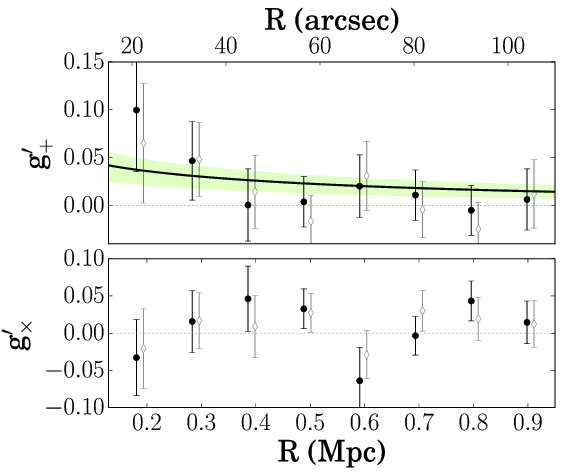
The weak lensing signal is expressed as the tangential component of the shear . The cross component , defined as after the object is rotated by and represents the null statistic and noise of our measurements and should be consistent with zero in the absence of systematic errors.
We determine the shear as a function of cluster radius by radially binning our catalog objects and calculating the average and of all objects in each bin. The cluster center is at the location of the BCG (RA= and Dec=). The shear profile is plotted in Figure 3 where the error bars shown for the shear measurements are the statistical uncertainty of the mean shear per bin. By adding in quadrature the ratio of mean shear and uncertainty per bin for the first six bins, we calculate a significance of for the detection. The Pearson’s correlation coefficient between the tangential and cross shear components is small (), indicating no correlation between the two components
As a test of robustness of this detection, we also employ an alternative shape measurement from the Jee et al. (2009, hereafter J09) and RRG methods. Using the same galaxy selection, we find that the shapes obtained using the J09 and RRG methods yield consistent results: the typical absolute difference between the mean measured values in each bin is within for the tangential shear and for the cross component.
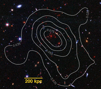
The J09 approach is designed to extend to faint magnitudes. With this method, we also perform a 2-D mass reconstruction using a more relaxed set of selection criteria. Specifically, we allow a wider range in magnitudes (F606W and F160W), a relaxed red sequence selection (F814W-F160W), and a decreased size selection (F606W half-light radius ). The centroid of the resulting 2-D mass reconstruction is close to the location of the BCG, providing further evidence that the shear is the result of the cluster weak lensing. The shear contours are overplotted on the HST image in Figure 4. Finally, we note that the tangential shear profile using this different selection remains consistent with Figure 3 but with smaller statistical uncertainties. We continue the analysis with our original shape measurement.
5. Mass Estimation
The tangential shear is related to the density profile of the cluster assuming a Navarro-Frenk-White (NFW) profile (Navarro et al., 1997) described by the virial radius , defined as the radius inside which the mass density of the halo is equal to times the critical density, and the concentration , where is the scale radius. For the radial dependence of the shear in an NFW model, we refer the reader to Equations of Wright & Brainerd (2000).
To fit the shear profile, we utilize the maximum likelihood estimation discussed in Schneider et al. (2000). The log-likelihood function is defined as
| (5) |
where is the number of galaxies with measured ellipticity, is the tangential ellipticity component, is the position of the -th galaxy, and is the observed tangential shear at . The dispersion of observed ellipticities approximated as , the same as that defined in Equation 14 of Schneider et al. (2000), where is the intrinsic ellipticity dispersion.
We lack the necessary signal to fit the mass and concentration simultaneously as free parameters. Thus, we derive the cluster mass with the concentration defined by the mass-concentration relation from Duffy et al. (2008),
| (6) |
where the mass within is . In this case, is the only free parameter in the likelihood fit, and the resultant value can be applied to directly compare IDCS J1426.5+3508 with the SZ-lensing relation defined by low redshift clusters. All objects located at radii ( kpc) are included in our fit (802 sources). We exclude the strong lensing region, defined by the radius of the known strongly-lensed arc (Gonzalez et al., 2012), and extend to a radius that best constrains the mass confidence interval. We derive M⊙ () which corresponds to Mpc ( Mpc). Changing the center to that of the X-ray observations (Brodwin et al., 2015) yielded a mass within of the mass derived with BCG centering. The NFW profile described by our best-fit parameters is plotted in Figure 3.
IDCS J1426.5+3508 is the only galaxy cluster in this regime to have joint weak lensing, strong lensing, SZ, and X-ray observations. Brodwin et al. (2015) find good agreement between the mass estimations from X-ray, SZ, and strong lensing. Converting from to via the Duffy et al. (2008) relation, Brodwin et al. (2012) calculate an SZ mass M⊙, Brodwin et al. (2015) estimate a mass from the X-ray gas mass of M⊙, while Gonzalez et al. (2012) projected a lower limit of M⊙ from observations of the giant arc. Our weak lensing mass of M⊙ falls at the lower end of these mass estimates but is consistent.
6. SZ-Weak Lensing Scaling Relation
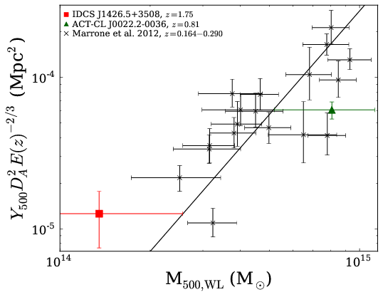
The SZ Compton parameter scales with mass as where is the angular diameter distance and is the evolution of the Hubble parameter. We combine our weak lensing-derived mass estimate with the spherically averaged dimensionless Comptonization parameter () from Brodwin et al. (2012) to compare IDCS J1426.5+3508 with the mass- scaling relation derived by Marrone et al. (2012) using 18 Local Cluster Substructure Survey (LoCuSS) clusters in the range . Figure 5 shows our results alongside the Marrone et al. (2012) sample and scaling relation. In this figure, we match the CDM cosmology assumed by Marrone et al. (2012, , , km s-1 Mpc-1). We also include the ACT-CL J0022.2-0036 at (Miyatake et al., 2013; Reese et al., 2012), a higher redshift cluster with comparable SZ and weak lensing observations, for comparison.
Our results for IDCS J1426.5+3508 are statistically consistent with the low redshift data, indicating minimal redshift evolution in the Marrone et al. (2012) scaling relation. To quantify the redshift evolution, we fit a regression of the form
| (7) |
where is the average redshift of the LoCuSS sample and and are regression coefficients from Marrone et al. (2012). Including the data for the LoCuSS clusters individually, ACT-CL J0022.2-0036, and IDCS J1426.5+3508, a least-squares fit yields , within of zero. Thus, we find no significant evidence for evolution in the Marrone et al. (2012) scaling relation.
7. Conclusions
We have presented the weak lensing analysis of IDCS J1426.5+3508. At , this is the highest redshift galaxy cluster to be studied through weak lensing. We detect a tangential shear signal at a -level significance. Assuming an NFW profile and a Duffy et al. (2008) mass-concentration relation, we fit for the cluster mass with a maximum-likelihood algorithm. Our mass estimate M⊙ is in agreement with estimates from X-ray, SZ, and strong lensing data. We also find that the SZ and weak lensing mass estimates agree well with the local scaling relation of Marrone et al. (2012), with negligible evolution in the relation.
Gonzalez et al. (2012) initially discovered the strong-lensed arc behind IDCS J1426.5+3508. If one makes standard assumptions for the galaxy cluster mass function, cosmological model, source galaxy redshift distribution, and cluster lensing cross section, then such an arc should not exist across the entire sky. The cluster lensing cross section increases with concentration, so one plausible explanation for this arc would be if the projected concentration of the cluster mass profile dramatically exceeds the typical value predicted for a cluster of this mass at this epoch. We are unable to determine a concentration as a free parameter for this cluster with the current data. However, a higher signal-to-noise weak lensing map and additional passbands to determine photometric redshifts would enable simultaneous fitting of the mass and concentration, improving Figure 3 and helping resolve the origin of the strong arc in this cluster.
Acknowledgments
The authors thank the anonymous referee and Daniel Stern for their insightful suggestions and Audrey Galametz for her help with the CANDELS-UDS data. Support for HST GO-program 11663, 12203, and 12994 was provided by NASA through a grant from the Space Telescope Science Institute, which is operated by the Association of Universities for Research in Astronomy, Inc., under NASA contract NAS 5-26555. We also acknowledge funding received from the National Science Foundation Graduate Research Fellowship under Grant No. DGE-1315138 (W.M.), NRF of Korea to CGER (M.J.J.), and Royal Society University Research Fellowship (R.M.). J.R. is supported by JPL, which is run by Caltech under a contract for NASA.
References
- Alberts et al. (2014) Alberts, S., Pope, A., Brodwin, M., et al. 2014, MNRAS, 437, 437
- Bayliss et al. (2014) Bayliss, M. B., Ashby, M. L. N., Ruel, J., et al. 2014, ApJ, 794, 12
- Bertin & Arnouts (1996) Bertin, E., & Arnouts, S. 1996, A&AS, 117, 393
- Bleem et al. (2015) Bleem, L. E., Stalder, B., de Haan, T., et al. 2015, ApJS, 216, 27
- Brodwin et al. (2015) Brodwin, M., McDonald, M., Gonzalez, A. H., et al. 2015, ArXiv e-prints, arXiv:1504.01397
- Brodwin et al. (2012) Brodwin, M., Gonzalez, A. H., Stanford, S. A., et al. 2012, ApJ, 753, 162
- Brodwin et al. (2013) Brodwin, M., Stanford, S. A., Gonzalez, A. H., et al. 2013, ApJ, 779, 138
- Bruzual & Charlot (2003) Bruzual, G., & Charlot, S. 2003, MNRAS, 344, 1000
- Duffy et al. (2008) Duffy, A. R., Schaye, J., Kay, S. T., & Dalla Vecchia, C. 2008, MNRAS, 390, L64
- Eisenhardt et al. (2008) Eisenhardt, P. R. M., Brodwin, M., Gonzalez, A. H., et al. 2008, ApJ, 684, 905
- Fassbender et al. (2011) Fassbender, R., Böhringer, H., Nastasi, A., et al. 2011, New Journal of Physics, 13, 125014
- Gonzalez et al. (2012) Gonzalez, A. H., Stanford, S. A., Brodwin, M., et al. 2012, ApJ, 753, 163
- Hinshaw et al. (2013) Hinshaw, G., Larson, D., Komatsu, E., et al. 2013, ApJS, 208, 19
- Hoekstra et al. (2012) Hoekstra, H., Mahdavi, A., Babul, A., & Bildfell, C. 2012, MNRAS, 427, 1298
- Jee et al. (2007) Jee, M. J., Blakeslee, J. P., Sirianni, M., et al. 2007, PASP, 119, 1403
- Jee et al. (2009) Jee, M. J., Rosati, P., Ford, H. C., et al. 2009, ApJ, 704, 672
- Jee et al. (2011) Jee, M. J., Dawson, K. S., Hoekstra, H., et al. 2011, ApJ, 737, 59
- Krist & Hook (1997) Krist, J. E., & Hook, R. N. 1997, in The 1997 HST Calibration Workshop with a New Generation of Instruments, ed. S. Casertano, R. Jedrzejewski, T. Keyes, & M. Stevens, 192
- Krist et al. (2011) Krist, J. E., Hook, R. N., & Stoehr, F. 2011, in Society of Photo-Optical Instrumentation Engineers (SPIE) Conference Series, Vol. 8127, Society of Photo-Optical Instrumentation Engineers (SPIE) Conference Series
- Leauthaud et al. (2007) Leauthaud, A., Massey, R., Kneib, J.-P., et al. 2007, ApJS, 172, 219
- Marrone et al. (2012) Marrone, D. P., Smith, G. P., Okabe, N., et al. 2012, ApJ, 754, 119
- Massey et al. (2010) Massey, R., Stoughton, C., Leauthaud, A., et al. 2010, MNRAS, 401, 371
- Massey et al. (2014) Massey, R., Schrabback, T., Cordes, O., et al. 2014, MNRAS, 439, 887
- Meneghetti et al. (2013) Meneghetti, M., Bartelmann, M., Dahle, H., & Limousin, M. 2013, Space Sci. Rev., 177, 31
- Miyatake et al. (2013) Miyatake, H., Nishizawa, A. J., Takada, M., et al. 2013, MNRAS, 429, 3627
- Muzzin et al. (2013) Muzzin, A., Wilson, G., Demarco, R., et al. 2013, ApJ, 767, 39
- Navarro et al. (1997) Navarro, J. F., Frenk, C. S., & White, S. D. M. 1997, ApJ, 490, 493
- Newman et al. (2014) Newman, A. B., Ellis, R. S., Andreon, S., et al. 2014, ApJ, 788, 51
- Oke & Gunn (1983) Oke, J. B., & Gunn, J. E. 1983, ApJ, 266, 713
- Oke et al. (1995) Oke, J. B., Cohen, J. G., Carr, M., et al. 1995, PASP, 107, 375
- Papovich et al. (2010) Papovich, C., Momcheva, I., Willmer, C. N. A., et al. 2010, ApJ, 716, 1503
- Reese et al. (2012) Reese, E. D., Mroczkowski, T., Menanteau, F., et al. 2012, ApJ, 751, 12
- Rhodes et al. (2000) Rhodes, J., Refregier, A., & Groth, E. J. 2000, ApJ, 536, 79
- Rhodes et al. (2007) Rhodes, J. D., Massey, R. J., Albert, J., et al. 2007, ApJS, 172, 203
- Santini et al. (2014) Santini, P., Ferguson, H. C., Fontana, A., et al. 2014, ArXiv e-prints, arXiv:1412.5180
- Schneider et al. (2000) Schneider, P., King, L., & Erben, T. 2000, A&A, 353, 41
- Schrabback et al. (2010) Schrabback, T., Hartlap, J., Joachimi, B., et al. 2010, A&A, 516, A63
- Seitz & Schneider (1997) Seitz, C., & Schneider, P. 1997, A&A, 318, 687
- Stanford et al. (2012) Stanford, S. A., Brodwin, M., Gonzalez, A. H., et al. 2012, ApJ, 753, 164
- Tozzi et al. (2015) Tozzi, P., Santos, J. S., Jee, M. J., et al. 2015, ApJ, 799, 93
- Tran et al. (2010) Tran, K.-V. H., Papovich, C., Saintonge, A., et al. 2010, ApJ, 719, L126
- Vikhlinin et al. (2009) Vikhlinin, A., Burenin, R. A., Ebeling, H., et al. 2009, ApJ, 692, 1033
- Webb et al. (2015a) Webb, T., Noble, A., DeGroot, A., et al. 2015a, ApJ, 809, 173
- Webb et al. (2015b) Webb, T., Muzzin, A., Noble, A., et al. 2015b, ArXiv e-prints, arXiv:1508.07302
- Wright & Brainerd (2000) Wright, C. O., & Brainerd, T. G. 2000, ApJ, 534, 34
- Wylezalek et al. (2014) Wylezalek, D., Vernet, J., De Breuck, C., et al. 2014, ApJ, 786, 17
- Zeimann et al. (2012) Zeimann, G. R., Stanford, S. A., Brodwin, M., et al. 2012, ApJ, 756, 115