Automatic calibration of damping layers in finite element time domain simulations
Abstract
Matched layers are commonly used in numerical simulations of wave propagation to model (semi-)infinite domains. Attenuation functions describe the damping in layers, and provide a matching of the wave impedance at the interface between the domain of interest and the absorbing region. Selecting parameters in the attenuation functions is non-trivial. In this work, an optimisation procedure for automatically calibrating matched layers is presented. The procedure is based on solving optimisation problems constrained by partial differential equations with polynomial and piecewise-constant attenuation functions. We show experimentally that, for finite element time domain simulations, piecewise-constant attenuation function are at least as efficient as quadratic attenuation functions. This observation leads us to introduce consecutive matched layers as an alternative to perfectly matched layers, which can easily be employed for problems with arbitrary geometries. Moreover, the use of consecutive matched layers leads to a reduction in computational cost compared to perfectly matched layers. Examples are presented for acoustic, elastodynamic and electromagnetic problems. Numerical simulations are performed with the libraries FEniCS/DOLFIN and dolfin-adjoint, and the computer code to reproduce all numerical examples is made freely available.
Introduction
Three types of boundary conditions are frequently used in numerical wave propagation problems: reflecting boundaries, modelled by homogeneous Dirichlet and Neumann conditions; ports through which energy enters or leaves the system, modelled by non-homogeneous Dirichlet or Neumann boundary conditions; and boundary conditions that mimic open space when truncating an infinite domain. A number of strategies for truncating infinite domains have been developed, including absorbing boundary conditions [15, 26], absorbing layers [17, 20] and one-way approximations [10, 23]. An absorbing layer introduces damping and is realised by extending the computational domain beyond the domain of interest, and it is desirable to keep the size of the absorbing domain as small as possible to limit the additional computational work. However, none of the early damping layer techniques proved to be flawless.
In 1994, Bérenger [4] introduced an absorbing domain called Perfectly Matched Layers (PMLs). In a PML, waves are damped at a certain rate, described by an attenuation function (AF). It is desirable to use an ‘optimal’ AF in order to limit the size of the PML. Unfortunately, there is no universal recipe available to determine the best AF for specific problems. For particular cases, optimal PMLs can be found through mathematical analysis. For example, Chew and Jin [7] proved that for finite difference time domain methods, second-order polynomial AFs are optimal and suggested that these results should also be expected for finite element time domain methods. A generalisation of the analysis to more complicated cases (unstructured meshes, more general geometries and loads) is not straightforward, may be suboptimal or may even fail.
In this work we present an automatic calibration procedure for PMLs through optimisation of the PML parameters for a given problem. The functional we attempt to minimise is the energy left in the domain after an input signal should have left the domain of interest. The problem is constrained by the considered differential equation that describes the wave propagation of interest. We use gradient-based optimisation procedures to determine the parameters, with the adjoint of the forward problem used to compute the derivative of the target functional with respect to the PML parameters. We consider polynomial and piecewise-constant AFs, with the latter case motivating the introduction of what we will call ‘Consecutive Matched Layers’ (CMLs). An advantage of CMLs is that they are easily added to problems with arbitrary geometries, as we will show through numerical examples.
Numerical examples of the proposed procedure are presented for acoustic, elastodynamic and electromagnetic problems. The examples use the FEniCS/DOLFIN [21, 22, 2] and dolfin-adjoint [12, 13] libraries. The complete source code to produce the presented examples is freely available and provided as supporting material [30].
The remainder of the paper is organised as follows. The considered wave propagation problems are described in Section 2, followed by the introductions of PMLs in Section 3. In Section 4, the formulation of Consecutive Matched Layers (CMLs) is presented, which is followed by the proposed procedure for automatic calibration of PMLs and CMLs in Section 5. We present and discuss test cases and results in Section 6. Conclusions are drawn in Section 7.
Wave propagation problems
We will consider acoustic, elastodynamic and electromagnetic wave propagation problems. Each of these problems is defined in this section, but we first present a generic formulation in which these problems can framed.
On a spatial domain , where , we consider linear wave propagation problems in the generic form
| (1) |
where is a vector of length containing the unknown fields, is a flux vector of length , is a source function of length and is the final time. The matrices contain material parameters and will be defined for each specific problem we consider. The notation (no summation) implies component-wise partial differentiation of with respect to . Boundary conditions will be presented later for each specific problem.
The first considered model is acoustic wave propagation, described by the system
| (2) | ||||
where is the bulk modulus, is the pressure, is the velocity, is the mass density and is an applied body force. This problem is transformed into the generic form (1), in three-dimensions, with and the matrices in (31).
The second model concerns electromagnetic wave propagation, described by the system
| (3) | ||||
where is the permeability, is the magnetic field strength, is the electric field strength, is the permittivity and is a current density. This problem is transformed into the generic form (1), in three dimensions, with and the matrices in (34).
Finally, linearised elastic wave propagation will be considered, and is described by the system
| (4) | ||||
where is the fourth-order, isotropic elastic stiffness tensor, is the stress tensor, is the particle velocity, the mass density and is an applied body force. This problem is transformed into the generic form (1), in three dimensions, with and the matrices in (37).
Perfectly matched layers
We denote the domain of physical interest by , which is extended with an absorbing domain (), leading to the computational domain . To obtain a formulation for wave propagation problems with PMLs, we apply the technique of complex coordinate stretching [8, 28] to the generic wave equation in (1).
Solutions to wave equations are of the form
| (5) |
where is the spatial solution and is the frequency. A frequency domain formulation can be used by noting that . PMLs in all directions are applied by introducing the coordinate transformations
| (6) |
where are attenuation functions (AFs), and which are non-zero only in the absorbing region . The AFs will be defined at the end of the section.
We will denote combinations of different AFs in the index, e.g. . Using (5) and applying the coordinate transformations in (6) to the wave equation (1) leads to
| (7) |
Multiplying (7) by all denominators appearing in it leads to
| (8) |
With no source term inside the absorbing region , we have and the right-hand side of (8) simplifies to . Expanding the remaining products leads to
| (9) |
To obtain a system of first-order equations from (9), for two auxiliary fields, and are introduced, resulting in two auxiliary differential equations (ADEs) in addition to the wave equation:
| (10) | ||||
In two spatial dimensions () , we have the simplified system:
| (11) | ||||
In one spatial dimension (), there are no ADEs needed to describe the PML:
| (12) |
A specific PML is defined by the AFs . The literature, e.g. [7], generally suggests polynomial AFs. For axis-aligned rectangular (cuboid) domains, polynomial AFs can be expressed as
| (13) |
where is the order of the polynomial, are the coefficients of the polynomial, is an affine transformation of such that on the boundary between the domain of interest and the absorbing region, and on the exterior boundary of the absorbing region, is the interface between and and is the total width of the PML in the th direction.
We also introduce a description of an AF with piecewise-constant AFs of the form
| (14) |
where are scalar values and .
Consecutive matched layers
The complex coordinate stretching procedure used in the previous section to the PML configuration depicted in Figure 1a. Overlapping PML regions leads to products of AFs that appear in the ADEs in (10). Solving for the auxiliary fields adds to the computational cost. To avoid this increase in cost, we adopt a simplification to the PML strategy.
When using non-overlapping absorbing domains, as depicted in Figure 1b, products of AFs are zero and (10) reduces to
| (15) | ||||
which eliminates one ADE compared to (10). If we assume that , which can be motivated by the fact that spatial derivatives in the second equation will be relatively small due to the damping, also the second ADE vanishes, further reducing (10) to
| (16) |
Since we prefer direction-independent AFs, we choose the AF in all directions to be defined by the same constant. Hence, can be replaced by an AF of the form
| (17) |
where is a constant scalar and is the th ‘layer’ of the absorbing domain. Using the AF in (17) for a problem where leads to a simplification of (16):
| (18) |
This formulation closely resembles the original absorbing layer strategy [17]. We however suggest to consider an absorbing domain which is divided into non-overlapping absorbing layers such that , which leads to the formulation
| (19) |
The resulting configuration is illustrated in Figure 1c, where the AF is constant on each colour/layer. Due to the absence of auxiliary fields, the computational cost is reduced relative to the PML model. A difficulty is how to choose the terms that define the AFs in the layers. This issue will be addressed in the following section.
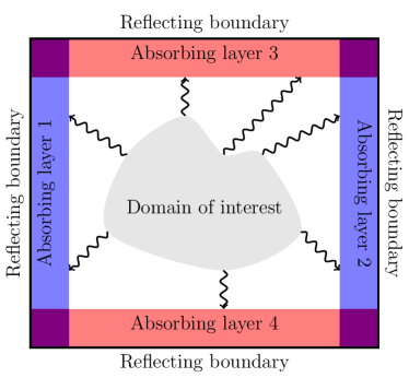
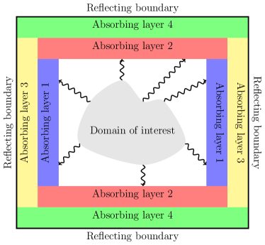
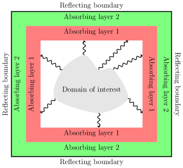
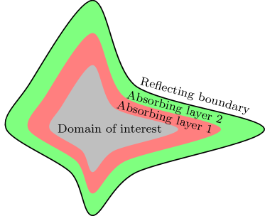
We note that a reasonable domain of interest can be extended with tightly wrapped layers, as shown in Figure 1d, and meshed conformingly. Hence this procedure can be applied to problems with arbitrary geometries, while avoiding complex mathematical interventions, e.g., as presented in [14].
By neglecting the ADE in (15) the absorbing domain is no longer a PML, hence we will refer to the simplified damping strategy as consecutive matched layers (CMLs). This name refers to the non-reflective free space boundary condition introduced in Katz et al. [20], mentioned as absorbing layer in Holland and Williams [17] and referred to as matched layer in Bérenger [4].
Automatic calibration of matched layer problems
The matched layer approaches presented in the preceding sections involved scalar AFs, , and it is necessary to define their functional form. For finite difference methods, there are numerous papers describing how to determine the AFs, e.g, [3, 7, 9]. Chew and Jin [7] proved that quadratic polynomials result in optimal AFs for finite difference methods. Even if we presume that quadratic polynomial AFs are optimal for finite element time domain simulations, the question remains what precise form the quadratic polynomial should take for optimal results. Since users often want to add damping layers to their models without studying the truncation strategy in depth, an automatic determination procedure is appealing. We present a generic recipe for automatic calibration of the AF coefficients. The presented procedure is based on solving an optimisation problem.
Formulation of the optimisation problem
Our abstract optimisation problem is formulated as
| (20) | ||||
| (21) |
where is a scalar function, is the state vector, is the control vector, is the set of the admissible values for the control values and represents a set of constraints. For the considered problems, the state vector contains in the wave equation (1), and in the case of PML calibration is also contains the solutions of the auxiliary fields and in (10). The control vector contains the parameters that define the AFs. Satisfaction of the constraint in our case is satisfaction of the wave equation with matched layers.
The matched layer optimisation problem is in general not convex due to the non-linear relation between the controls and the states given by the constraint. This implies the likely existence of multiple local minima. Consequences of the existence of multiple local minima will be demonstrated by the numerical examples in Section 6. This prohibits us of considering the outcome of the automatic calibration procedure as optimal. Based on experimental results, we will however argue that the outcome is very likely to have near optimal performance.
Measuring the quality of the absorbing region
To define an objective functional we need to quantify the quality of a matched layer problem. Typical quality measures involve the reflection coefficients, both at the interface between the domain of interest and the matched layer , and within the matched layer (see [7]). This a priori quality measure is difficult to manipulate in combination with finite element formulations.
We propose quantifying the quality of a matched layer through the amount of energy in a system at judiciously chosen time for a judiciously chosen source term. With reflecting boundaries around the domain of interest and a vanishing input signal, the total energy in the system for the considered problems is constant once the input signal has vanished. If the domain of interest was embedded in an infinite domain, the total energy in the domain of interest would be zero at sufficiently large time. When absorbing layers are added to the domain of interest to mimic an infinite domain, the energy will reduce over time due to attenuation in the absorbing layers only, but it is highly unlikely that it will ever be exactly zero. The goal of the calibration procedure is to choose parameters for the matched layers such that the energy in the whole computational domain is minimised at a suitably chosen time, which we will call the ‘calibration time’, . The reduction in energy in the numerical simulation at time due to the absorbing layers is given by
| (22) |
where , the energy in the whole computational domain with zero-valued AFs, is used as a reference value and is the energy on the computational domain for the problem with non-zero AFs.
Objective functional
The objective functional we use in calibrating matched layer problems is
| (24) |
where is the energy in the system at the calibration time.
Another quantity of interest in designing matched layers is reflections at the interface between the domain of interest and the damping region. If the calibration time is chosen too large, then energy can be damped gradually every time a wave encounters the damping region and is partially reflected by it. In order to include the effect of these reflections in (24), the calibration time should be chosen such that reflections of the input signal at the material/matched layer interface encounter the damping region as few times as possible.
A practical concern is that the calibration time should be chosen as small as possible for computational speed, since a greater calibration time increases the number of time steps, and hence the cost of the optimisation process.
Computing derivatives of the objective functional
We will use derivative-based optimisation methods to calibrate the matched layer parameters. To compute the gradient of the objective functional with respect to the control parameters , we use the adjoint approach [29]. In essence, we find from
| (25) |
where the adjoint variable is the solution to:
| (26) |
A detailed derivation for the time discretised problems can be found in C. Key to the adjoint approach for computing derivatives of functionals is that that only one system needs to be solved to compute the gradient, regardless of the number of controls. Moreover, (26) is similar in structure to the system that is solved in the forward problem.
Practical procedure
To automatically calibrate a PML or CMLs for a problem of interest we create a calibration set-up. The procedure is:
-
1.
Extend the domain of interest with artificial layers and mesh domain with cell edges conforming to the boundary of and .
-
2.
Extend the physical material parameters on the domain of interest to the absorbing region.
-
3.
Set the attenuation in the damping region to zero.
-
4.
Select an input signal with local support in time to fit the frequency range of the application under consideration.
-
5.
Select a calibration time , such that the peak of the input pulse has travelled at least once through the damping region in every direction at the lowest wave speed.
-
6.
Update the AF parameters via a gradient-based optimisation process.
When the optimiser has converged, the obtained controls for the calibration set-up are used in the AF to solve the forward problem of interest. Note that the calibration set-up can differ from the problem of interest, as will be demonstrated for the electromagnetic example in Section 6. In the other example the geometry, mesh and excitation of the problem of interest and calibration set-up are kept. The final time of the problem of interest can differ from the calibration time, . We will call the final time for the problem of interest the ‘evaluation time’, .
Numerical examples and discussion
We present examples using the calibration procedure for finite element acoustic, elastic and electromagnetic wave propagation problems, and consider both PMLs and CMLs. We will begin with a one-dimensional example, before moving on to two- and three-dimensional cases to examine performance with oblique incidence angles. We will consider PMLs for acoustic and elastodynamic examples, and CMLs for elastodynamic and electromagnetic examples. The computer code for reproducing all examples is available in the supporting material [30].
For all examples, we use the L-BFGS-B optimiser from SciPy [19]. This optimiser is a limited memory BFGS implementation with bound support [6]. The bound support is used to prevent the optimiser choosing negative values for the piecewise-constant AFs. The optimiser stops when the gradient drops below a chosen threshold [25]. The threshold used in the different examples can be found in the supporting material [30].
To fully define the objective functional in (24), a calibration time and input signal have to be chosen. For all examples we use a Gaussian pulse. We choose the calibration time such that the peak of the input pulse has time to travel at least once to the boundary of the computational domain and back to the interface between the domain of interest and the absorbing domain at the lowest wave speed. Unless mentioned otherwise, first-order elements are used for all computations.
Perfectly matched layers
The examples presented in this section consider polynomial and piecewise-constant AFs for PMLs, as described in Section 3.
Acoustic wave propagation
We consider a rectangular domain of interest , which is extended at the right-hand boundary with a PML, as depicted in Figure 2. The domain is meshed with crossed-triangle cells with edge length in both - and -directions. Periodic boundary conditions are applied in the -direction. On the right-hand side of the computational domain, a reflecting boundary condition with is applied. An open boundary on the right-hand side of the domain is modelled by adding a PML in front of the reflecting boundary. On the left-hand boundary, the condition is applied, where is the offset for the pulse. Note that for a large enough time approaches zero and this boundary acts as a reflecting fixed boundary.

We consider a homogeneous medium with mass density and bulk modulus . The time step is 90% of the CFL condition, , where is the wave speed for the medium. The offset of the pulse is chosen to be . The calibration time is chosen to be the time the peak of the pulse needs to travel two and a half times through the domain of interest, . This way the peak of the pulse can encounter the PML interface only once, but there is sufficient time for the pulse to travel back-and-forth in the PML. For this example the calibration set-up is identical to the problem of interest, including the evaluation time .
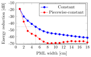
We first compare constant with piecewise-constant AFs for different PML widths. The smallest considered PML is wide. The PML is extended in -direction seventeen times, up to a total width of . When a piecewise-constant AF is considered, one control value is added for every extension, e.g., for a wide PML, the piecewise-constant AF is defined by five control variables. The energy reduction, as defined in (22), for these experiments with the calibrated AFs is shown in Figure 3a. These results show that piecewise-constant AFs perform better than constant AFs for every PML width.
The reduction in energy for different polynomial order AFs and different PML widths is shown in Figure 3b. First note the results for the fourth-order polynomial AF, where the PML appears to outperform the PML. This peculiarity points to the optimisation problem being non-convex. We will comment on this further when examining initial guesses for the controls. Comparing Figure 3a and Figure 3b, it can be concluded that piecewise-constant AFs outperform the polynomial AFs, e.g., for a wide PML, the calibrated piecewise-constant AF reduces the energy more than any polynomial AF. We note from Figure 3b that there appears to be limited benefit in using polynomial orders greater than two, which is consistent with finite difference results presented by Chew and Jin [7]. We restrict further experiments to AFs to polynomial degrees of two or less.
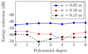
We would expect the performance of a polynomial AF to be at least as good as the constant AF case since the polynomial case contains the constant case. However, Figure 3b shows that for a wide PML, a constant AF is slightly more effective than any other polynomial AF. This again points to the optimisation problem being non-convex.
We now fix the PML width to to examine the influence of the initial AF parameters. Figure 4 shows the reduction in energy after optimisation for zero initial values (index ) and random starting values (indices greater than zero) for both a piecewise-constant and a quadratic AF. The starting values are uniformly sampled on the interval for the piecewise-constant case and the interval for the polynomial case. For the polynomial case, we allow negative coefficients in order to allow AFs that are not monotonically increasing. For the piecewise-constant AFs, the energy reduction for approximately ten percent of the results is more than from the best result. There is less variation in the computed energy reduction for quadratic AFs compared to the piecewise-constant case. However, every piecewise-constant AF outperforms all quadratic AFs. In the remainder we will set the initial guess for all controls to zero.
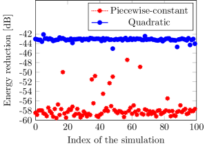
Figure 5 shows the piecewise-constant AF for , , , and wide PMLs. The result is not immediately intuitive; the first control value is relatively large, followed by a substantially smaller second control value. The remaining control values are approximately equal and larger than the second value. The counter-intuitive outcome highlights an advantage of using an optimisation approach.
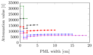
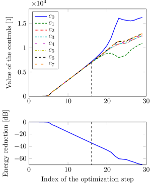
Figure 6 shows how the control values of the piecewise-constant AF change with each optimiser iteration for a wide PML together with the corresponding reduction in energy. For up to approximately 17 iterations the process favours a constant AF. From the point at which the AF deviates significantly from a constant AF, a further to reduction in energy is observed.
Elastodynamic wave propagation on a square
We simulate elastic wave propagation in an isotropic, homogeneous square domain , which is extended in both the - and -directions with a wide PML (see Figure 7a). We implement reflecting fixed boundaries on all sides of the computational domain. The longitudinal wave speed in the considered medium is and the transverse wave speed . The mass density of the considered material is . A Gaussian source is applied, where
| (27) |
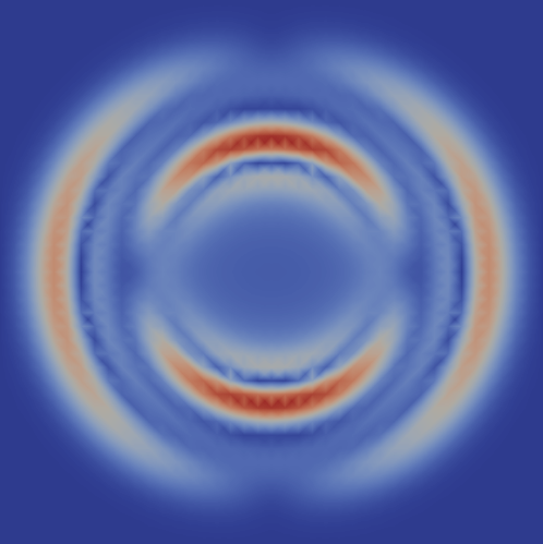
A typical resulting elliptical wave front for this example is illustrated in Figure 7b.
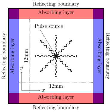
The domain is meshed with crossed-triangle cells with edge length . We solve this example using a discontinuous Galerkin finite element method, which is presented in B.2. A time step size of is used. The calibration time is chosen to be , which is the time needed for the peak to enter the domain and travel to the corner of the computational domain at the lowest wave speed. We consider the problem of interest to be identical to the calibration set-up with the exception of the evaluation time. Since the calibration time doesn’t allow the wave to travel once in both direction through the absorbing layer, the reduction in energy would not include the full benefit of the absorbing layer. The evaluation time for this example is , which is the calibration time plus the time needed for the peak to travel back from the corner of the computational domain to the centre of the domain.
This model uses one AF in each spatial direction. It is however undesirable to have orientation dependent PMLs because of the symmetry of the domain. We therefore choose to define the AFs in both directions by the same control variables.
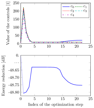
The evolution of the controls and reduction in energy at each optimiser step for the piecewise-constant case are shown in Figure 8. Despite the large changes in the control values at low iteration counts, the reduction in energy remains more-or-less constant from the second iteration. The final result is again not a monotonically increasing function, shown by the AF in Figure 9 (solid blue line).
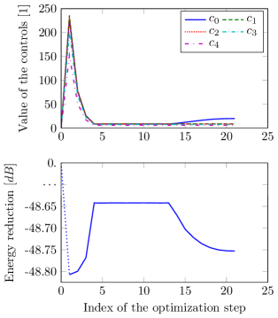
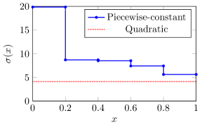
As a second experiment for this model, we compare the piecewise-constant result to a quadratic AF. The evolution of the controls and reduction in energy during the optimisation process for a quadratic AF are shown in Figure 10. The calibration process for a quadratic AF has resulted in a constant AF (see Figure 9) and performs about less well than the calibrated piecewise-constant AF.
Consecutive matched layers
We now move to examining the performance of the truncation strategy of consecutive matched layers presented in Section 4. In this case each ‘sub-layer’ has a constant attenuation function associated with it. The key difference with perfectly matched layers is the absence of auxiliary fields and equations in the model.
Elastodynamic wave propagation on a square
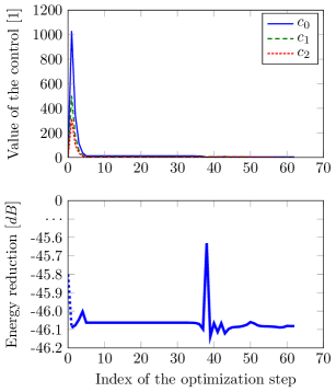
We revisit the elastodynamic example from Section 6.1.2. Both the problem of interest and the calibration set-up are identical to the previous example with the PML replaced by CMLs. The evolution of the controls and reduction in energy during the optimisation process for calibrating the five CMLs are shown in Figure 11. The results shown in Figure 11 are almost identical to the PML results in Figure 8. Since the model for CMLs does not require ADEs, in contrast to the PML model, the automatic calibration procedure for CMLs is faster than for PMLs.
Elastodynamic wave propagation on a more complicated geometry
We now adopt the problem of interest and calibration set-up of the preceding elastic example, but replace the square domain by the domain and mesh shown in Figure 12. The domain of interest is shown in dark blue. Five consecutive matched layers are placed around the domain of interest. The precise definition of the domain and the mesh are available in the supporting material [30].
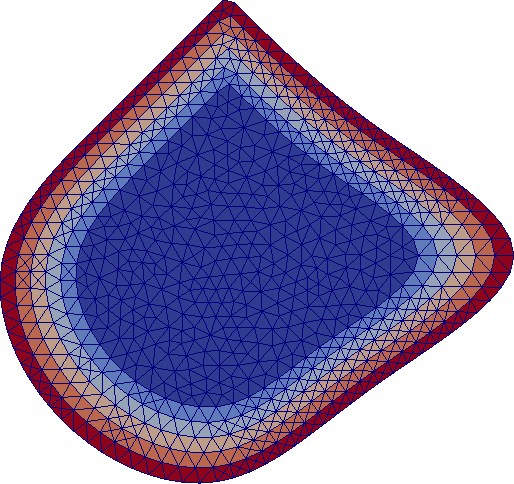
The evolution of the attenuation constants for this problem and the corresponding reduction in energy are shown in Figure 13. The reduction in energy is only ten percent less than for the problem on the square domain. The attenuation in layers closer to the domain of interest is larger than for the layers farther from the domain of interest. This is probably a manifestation of the sensitivity of the different controls. It is to be expected that the attenuation in the outer layers has less effect on the reduction in energy, since a considerable amount of energy will have been damped by layers closer to the domain of interest.
Electromagnetic wave propagation
We consider an application for which an absorbing region is calibrated, and then used to solve a problem of interest. The problem of interest involves a transverse electromagnetic wave [18] in a parallel plate wave guide. We solve equation (3) on the domain of interest . We consider conducting plates at and , which are both modelled by implementing perfect electric conducting boundary conditions () at and . The face at is a port through which waves are inserted into the wave guide. We consider the case where the plates are infinite in -direction, which is modelled by applying perfect magnetic conducting boundary conditions () at and . For there is open space, which will be modelled using CMLs.
Before solving the problem of interest we calibrate the AFs on the adsorbing layer. To study the impact of oblique incidence angles at the boundary of the domain of interest, we will ‘stretch’ the upper conducting plate () in the direction. Three configurations will be tested, i.e., with , and degree incidence angles. The domain with a degree incidence angle is shown in Figure 14. The volume of absorbing layers will slightly differ in all three cases due to the different plate lengths, but the thickness of each layer (in the -direction) is fixed.
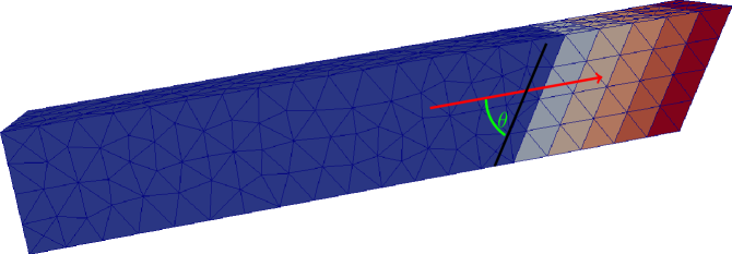
We extend the domain of interest with five absorbing layers, each one cell wide (see Figure 14). Also the boundary conditions of the domain of interest at , , and are extended to the absorbing domain. The boundary condition at the port () is set to , where
| (28) |
At the end of the CMLs () a perfect electric conducting boundary condition is applied. The calibration time is chosen to be the time for the peak of the input pulse to enter the system, move through the domain of interest, reflect off the interface between the domain of interest and the absorbing domain, and back to the source of the input signal, which is . To optimise the attenuation functions, we initialise the AFs to zero, and run the optimisation process for the , and degree incidence angle cases.
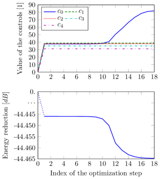
The evolution of the control variables and the corresponding reduction in energy at for the cases with , and degree incidence angles are shown in Figure 15. We see that the two cases with non-perpendicular incidence perform well relative to the to the degree case. The obtained attenuation values differ significantly between the three cases. The smaller the incidence angle, the more iterations are required to converge the optimisation algorithm.
We observe the least energy reduction for the degree incidence case. The observation that the degree incidence case performs better than both other cases is mainly because when a wave hits the interface between the domain of interest and the absorbing domain at a degree incidence angle, the wave is reflected to the upper plate, hits it perpendicularly and hence is reflected again at a forty-five degree angle to the CMLs, before it gets reflected again in negative -direction towards the source of the input signal. In other words, reflected waves meet the CMLs for a second time sooner than in the other cases.


To complete the electromagnetic wave case study, we compute a transverse electromagnetic wave in the wave guide with the degree incidence angle and the CMLs that were calibrated for this case. The boundary conditions are as described for the calibration set-up, except now as an input wave we apply the boundary condition at the port (), with
| (29) |
There is no analytical solution available for a transverse electromagnetic wave in a parallel plate wave guide where one plate is longer than the other. However, as the waves move from left to right in the wave guide, the solution in the rectangular part is not affected by the rest of the domain. Hence, we can use the analytical solution for a parallel wave guide with equal plates for which is
| (30) |
where is the speed of light and is the permeability of vacuum.
For the initial condition, it is not straightforward to extend the analytical solution (30) into the absorbing region. Therefore, we start with a zero initial value and compare the numerical solution to the analytical solution after the problem reaches a steady state. To evaluate the numerical solution, we compare the electromagnetic energy (defined in (35)) of the numerical solution computed with third-order polynomial elements to the reference solution in (30) in Figure 16. We see that, after reaching the steady state, the periods of the numerical and exact solutions are well aligned. Importantly, we see that there is no systematic increase in energy for the numerical case, which demonstrates that the CMLs are effective.

Conclusions
We have presented an approach to automatically calibrate attenuation functions for matched layers in wave propagation problems solved using finite element time domain methods. The presented procedure is not problem-specific, and in principle can be used to calibrate perfectly matched layers for any problem, regardless of the discretisation method. We have experimentally shown that there is no need to use polynomial attenuation functions higher than order two. Piecewise-constant attenuation functions can however result in equally effective perfectly matched layers. For piecewise-constant attenuation functions, the calibration procedure does not prefer monotonically increasing attenuation functions.
We have presented calibration of a damping strategy which we call consecutive matched layers. The automatic calibration procedure for consecutive matched layers is identical to the calibration procedure for perfectly matched layers. Consecutive matched layers lead to a simpler model than perfectly matched layers, resulting in shorter simulation times, for both the forward problem and the calibration procedure. It was shown for a collection of examples that consecutive matched layers can perform as well as perfectly matched layers. As a major advantage of consecutive matched layers over perfectly matched layers is that consecutive matched layers can be easily applied to complex domains.
Acknowledgements
The authors would like to acknowledge Febe Brackx for her help with the preliminary implementation and simulations, Patrick Farrell and Simon Funke for their assistance with dolfin-adjoint, Stefan Vandewalle, for helpful discussions on the content of this paper. Steven Vandekerckhove was been funded by a PhD grant from the Agency for Innovation by Science and Technology (IWT) and an international collaboration grant from the Research Foundation - Flanders (FWO).
References
References
- Alnæs et al. [2014] M. S. Alnæs, A. Logg, K. B. Ølgaard, M. E. Rognes, and G. N. Wells. Unified Form Language: A domain-specific language for weak formulations of partial differential equations. ACM Trans Math Software, 40(2):9:1–9:37, 2014.
- Alnæs et al. [2015] M. S. Alnæs, J. Blechta, J. Hake, J. Johansson, B. Kehlet, A. Logg, C. Richardson, J. Ring, M. E. Rognes, and G. N. Wells. The FEniCS Project Version 1.5. Archive of Numerical Software, 3(100):9–23, 2015.
- Asvadurov et al. [2003] S. Asvadurov, V. Druskin, M. Guddati, and L. Knizhnerman. On optimal finite-difference approximation of PML. SIAM Journal on Numerical Analysis, 41(1):287–305, 2003.
- Bérenger [1994] J.-P. Bérenger. A perfectly matched layer for the absorption of electromagnetic waves. Journal of Computational Physics, 114(2):185 – 200, 1994.
- Bou Matar et al. [2012] O. Bou Matar, P.-Y. Guerder, Y. Li, B. Vandewoestyne, and K. Van Den Abeele. A nodal discontinuous Galerkin finite element method for nonlinear elastic wave propagation. The Journal of the Acoustical Society of America, 131(5):3650–3663, 2012.
- Byrd et al. [1995] R. H. Byrd, P. Lu, and J. Nocedal. A limited memory algorithm for bound constrained optimization. SIAM Journal on Scientific and Statistical Computing, 16, 5:1190–1208, 1995.
- Chew and Jin [1996] W. C. Chew and J. M. Jin. Perfectly matched layers in the discretized space: An analysis and optimization. Electromagnetics, 16(4):325–340, 1996.
- Chew and Weedon [1994] W. C. Chew and W. H. Weedon. A 3-d perfectly matched medium from modified Maxwell’s equations with stretched coordinates. Micro. Opt. Tech. Lett., 7(13):599–604, 1994.
- Collino and Monk [1998] F. Collino and P. B. Monk. Optimizing the perfectly matched layer. Computer Methods in Applied Mechanics and Engineering, 164(1–2):157 – 171, 1998.
- Engquist and Majda [1977] B. Engquist and A. Majda. Absorbing boundary conditions for numerical simulation of waves. Proceedings of the National Academy of Sciences, 74(5):1765–1766, 1977.
- Etienne et al. [2010] V. Etienne, E. Chaljub, J. Virieux, and N. Glinsky. An hp-adaptive discontinuous Galerkin finite-element method for 3-D elastic wave modelling. Geophysical Journal International, 183(2):941–962, 2010.
- Farrell et al. [2013] P. E. Farrell, D. A. Ham, S. W. Funke, and M. E. Rognes. Automated derivation of the adjoint of high-level transient finite element programs. SIAM Journal on Scientific Computing, 35(4):C369–C393, 2013.
- Funke and Farrell [2013] S. W. Funke and P. E. Farrell. A framework for automated PDE-constrained optimisation. submitted, 2013. arXiv:1302.3894 [cs.MS].
- Gao and Zhang [2008] H. Gao and J. Zhang. Implementation of perfectly matched layers in an arbitrary geometrical boundary for elastic wave modelling. Geophysical Journal International, 174(3):1029–1036, 2008.
- Hagstrom [1999] T. Hagstrom. Radiation boundary conditions for the numerical simulation of waves. Acta Numerica, 8:47–106, 1999.
- Hesthaven and Warburton [2008] J. Hesthaven and T. Warburton. Nodal discontinuous Galerkin methods, volume 54 of Texts in Applied Mathematics. Springer, Berlin, 2008.
- Holland and Williams [1983] R. Holland and J. W. Williams. Total-field versus scattered-field finite-difference codes: A comparative assessment. Nuclear Science, IEEE Transactions on, 30(6):4583–4588, Dec 1983.
- Jackson [1998] J. D. Jackson. Classical Electrodynamics. Wiley, United States, 1998.
- Jones et al. [2001–] E. Jones, T. Oliphant, P. Peterson, et al. SciPy: Open source scientific tools for Python, 2001–. URL http://www.scipy.org/. [Online; accessed 2014-12-02].
- Katz et al. [1976] I. Katz, D. Parks, A. Wilson, M. Rotenberg, and J. Harren. Non-reflective free space boundary conditions for SGEMP codes. Systems, Science and Software, SSS-R-76-2934, May 1976.
- Logg and Wells [2010] A. Logg and G. N. Wells. DOLFIN: Automated finite element computing. ACM Trans Math Software, 37(2):20:1–20:28, 2010.
- Logg et al. [2012] A. Logg, K.-A. Mardal, and G. N. Wells, editors. Automated Solution of Differential Equations by the Finite Element Method, volume 84 of Lecture Notes in Computational Science and Engineering. Springer, 2012.
- Mur [1981] G. Mur. Absorbing boundary conditions for the finite-difference approximation of the time-domain electromagnetic-field equations. Electromagnetic Compatibility, IEEE Transactions on, EMC-23(4):377–382, Nov 1981.
- Nédélec [1980] J. C. Nédélec. Mixed finite-elements in . Numerische Mathematik, 35(3):315–341, 1980.
- Nocedal and Wright [2000] J. Nocedal and S. J. Wright. Numerical optimization. Springer, 233 Spring Street, New York, NY 10013, USA, second edition edition, 2000.
- Peterson [1988] A. F. Peterson. Absorbing boundary conditions for the vector wave equation. Microwave and Optical Technology Letters, 1(2):62–64, 1988.
- Raviart and Thomas [1977] P. A. Raviart and J. M. Thomas. Primal hybrid finite-element methods for 2nd-order elliptic equations. Mathematics of Computation, 31(138):391–413, 1977.
- Teixeira and Chew [2000] F. L. Teixeira and W. C. Chew. Complex space approach to perfectly matched layers: a review and some new developments. International Journal of Numerical Modelling: Electronic Networks, Devices and Fields, 13(5):441–455, 2000.
- Tröltzsch [2010] F. Tröltzsch. Optimal Control of Partial Differential Equations: Theory, Methods and Applications. American Methematical society, Providence, Rhode Island, 2010. Graduate Studies in Mathematics, Volume 112.
- Vandekerckhove [2016] S Vandekerckhove. Automatic calibration of damping layers in finite element time domain simulations, January 2016. URL http://dx.doi.org/10.5281/zenodo.45296.
- Yee [1966] K. S. Yee. Numerical solution of initial boundary value problems involving Maxwell’s equations in isotropic media. IEEE Trans. Antennas Propag., Vol. 14:302–307, 1966.
Appendix A Problem specific expressions
Acoustic wave propagation
The matrices for the acoustic wave problem read:
| (31) |
The energy functional for the acoustic wave problem reads:
| (32) |
The matrix in (23) for this problem reads:
| (33) |
Electromagnetic wave propagation
The matrices for the electromagnetic wave problem read:
| (34) |
The energy functional for the electromagnetic wave problems reads:
| (35) |
The matrix in (23) for this problem reads:
| (36) |
Elastodynamic wave propagation
The matrices for the elastodynamic wave problem read:
| (37) |
The energy functional for the elastodynamic wave problem reads:
| (38) |
The matrix in (23) for this problem reads:
| (39) |
where is the stiffness tensor with in Voigt notation. Note that the matrix is block diagonal for this case.
Appendix B Finite element formulations
This appendix contains the finite element formulations for the examples presented in Section 6. For the description of the continuous problems we refer to Section 2. Unless mentioned otherwise in the text of Section 6, linear elements are used in all cases.
Acoustic wave propagation
We consider the acoustic wave problem described in Section 6.1.1. Applying the complex coordinate stretching transformation (6), in the first dimension only, to (2) we get the continuous system
| (40) | ||||
The semi-discrete finite element problem of (40) reads: find and such that
| (41) | ||||
where the function space is the usual continuous Lagrange finite element space and is spanned by Raviart–Thomas elements [27]. We use the same polynomial order for both finite element spaces. The classical leapfrog scheme is used to advance in time.
Elastic wave propagation
We will use the discontinuous Galerkin finite element method for the elastodynamic example. Examples of a discontinuous Galerkin finite element methods for elastic wave propagation can be found in [5, 11].
The semi-discrete discontinuous Galerkin finite element formulation for the two-dimensional generic PML description (11) on a triangulation of the computational domain into overlapping cells , reads: find and such that for all triangles
| (42) | |||
where the notation implies component-wise partial differentiation of with respect to , is the outward normal unit vector to , is the numerical flux (defined below), and the used function space is
| (43) |
where is the space of polynomial functions of degree on a cell . We choose Lax–Friedrichs numerical fluxes [16, p. 34]) to complete the formulation:
| (44) |
where the ‘’ and ‘’ superscripts indicate the interior and exterior side of an interface and is the greatest wave speed occurring in the problem. The trapezoidal rule is used to advance in time. All boundary conditions are enforced weakly.
Electromagnetic wave propagation
The semi-discrete finite element formulation for the electromagnetic wave propagation problem reads: find and such that
| (45) | ||||
where the function spaces and are spanned by Raviart–Thomas elements [27] and Nédélec elements of the first kind [24], respectively. We use the same polynomial order for both kinds of the elements. The Yee scheme [31] is used to advance in time.
Appendix C Computing the gradient of the objective functional for the time discretised problem
Consider the generic wave equation with a PML in one spatial dimension as given in (12) to be discretised in time with the implicit trapezoidal rule, with one constant matched layer added:
| (46) |
where is the computed approximation for and the accent indicates a spatial derivative, i.e., . We introduce the vector containing the solution at each time step. To be able to study the procedure in detail, we will restrict the time integration to two steps. In that case the objective function is
| (47) |
and its derivative with respect to the state vector is
| (48) |
The system of constraints in this case consists of three equations:
| (49) | ||||
for which we can compute the Jacobian matrix
| (50) |
where is the identity matrix of size where is the length of . To determine this matrix, four non-trivial partial derivatives have to be computed. In general, all we need is
| (51) | ||||
where is a diagonal matrix with This information allows us to compute the adjoint states by solving
| (52) |
which in this case looks like
| (53) |
Solving this system by back substitution leads to
| (54) | ||||
which is identical to solving the forward problem (49) up to the variable names. In fact, by feeding to the forward solver as a source, the adjoint states will be computed in reversed order.
To obtain the gradient, all that remains is to multiply the forward and adjoint states:
| (55) |