Phase metrology with multi-cycle two-colour pulses

Abstract

Strong-field phenomena driven by an intense infrared (IR) laser depend on during what part of the field cycle they are initiated. By changing the sub-cycle character of the laser electric field it is possible to control such phenomena. For long pulses, sub-cycle shaping of the field can be done by adding a relatively weak, second harmonic of the driving field to the pulse. Through constructive and destructive interference, the combination of strong and weak fields can be used to change the probability of a strong-field process being initiated at any given part of the cycle. In order to control sub-cycle phenomena with optimal accuracy, it is necessary to know the phase difference of the strong and the weak fields precisely. If the weaker field is an even harmonic of the driving field, electrons ionized by the field will be asymmetrically distributed between the positive and negative directions of the combined fields. Information about the asymmetry can yield information about the phase difference. A technique to measure asymmetry for few-cycle pulses, called Stereo-ATI (Above Threshold Ionization), has been developed by [Paulus G G, et al2003 Phys. Rev. Lett. 91]. This paper outlines an extension of this method to measure the phase difference between a strong IR and its second harmonic.

Keywords: attosecond physics, above-threshold ionization, phase metrology

1 Introduction

Strong field processes such as high-order harmonic generation (HHG) and above threshold ionization (ATI) depend on the sub-cycle structure of the strong infrared (IR) field driving the process. By tailoring the sub-cycle structure of the field, one can control the processes. This can be done either by using very short laser pulses [1, 2, 3] or by mixing pulses with different colours [4, 5, 6]. HHG with few-cycle laser pulses has enabled the generation of isolated attosecond pulses [7] and in this case the process is controlled by changing the so-called carrier–envelope phase (CEP) [8, 9, 10, 11, 12]:

$$\bi{E}(t)=\bi{E}_{0}f(t)\sin(\omega t+\phi_{\mathrm{CEP}}),$$ (1)

where $f(t)$ describes the envelope of the pulse with respect to which $\phi_{\mathrm{CEP}}$ is measured.

The CEP relates the phase of the driving frequency to the envelope of the pulse and changing it may lead to the generation of one or two attosecond pulses if the duration is sufficiently short [13]. The rapid change of amplitude of a short pulse broadens the pulse frequency distribution and breaks the symmetrical distribution of electron paths between the positive and negative directions of the field [14, 15]. How this depends on the CEP is illustrated in figure 1.

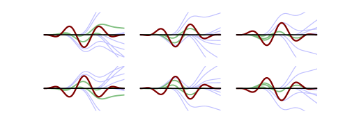
Figure 1: An illustration of the classical paths of electrons ionized by a few-cycle pulse, for six different CEPs. The green paths lead the electrons back to the atom, opening for the possibility of rescattering, whereas the blue paths guarantee direct ionization. The CEP of the driving field, shown in red, is changed by increments of $\frac{1}{3}\pi$ between each figure, giving phase difference of $\pi$ between the two pictures in each column. Note the asymmetry between the rows.

For two-coloured, multi-cycle fields with commensurate frequencies, the total electric is given by

$$\bi{E}(t)=\bi{E}_{1}\sin(\omega t)+\bi{E}_{2}\sin(n\omega t+\phi),$$ (2)

where $\bi{E}_{1},\bi{E}_{2}$ are the amplitudes of the fundamental frequency and its $n$th harmonic (in this letter, $n=2$), respectively, and $\phi$ is the relative phase between the two fields. The CEP is neglected in (2), since it has a negligible effect on the symmetry for multi-cycle pulses. Changing the relative phase of the two-coloured field may for instance result in one or two pulses per cycle [16] (see figure 2). One would assume that maximizing the asymmetry would also maximize the harmonic yield, since the harmonic yield scales with the field maximum, which is maximized at biggest asymmetry. However, SFA calculations showed [16] that there is a phase offset between maximum asymmetry and maximum harmonic yield and the highest harmonic cutoff. To truly understand and measure the impact of the sub-cycle structure, and enable the comparison between theory and experiment, the relative phase has to be measured independently from the process being studied and it has to be measured “on target”, where the harmonics are being generated.

Figure 2: A constant-amplitude field is shown together with its weaker, second harmonic for four different values of $\phi$. For each value of $\phi$ the first and the second harmonics are shown, in red and blue respectively, to the left, and their sum in purple to the right. To the right an interval corresponding to that in the left figure is shown in a darker colour.

For few-cycle pulses the phase is measured using a method known as Stereo-ATI [17, 18]. In Stereo-ATI the direction of the ionized electrons is measured and related to the CEP. In this letter we show that the Stereo-ATI technique can be used to measure the relative phase of a two-coloured field with commensurate frequencies and also the relative strength of the two fields, since varying $\phi$ has an impact on the field structure very similar to that of the CEP on short pulses [4].

1.1 Multi-cycle pulses

For multi-cycle pulses, the asymmetry due to variations in amplitude is very small from half-cycle to half-cycle. By approximating the amplitude as constant, the path of a directly ionized electron, leaving the atom at time $t_{0}$, can be seen as depending on the instant of ionization. This also decides its final energy, which is the same as the energy of an electron leaving the atom one half-cycle later, but in the opposite direction so that they do not overlap. The classical paths of electrons ionized by a strong one-coloured field are shown in figure 3(a). In this figure, the blue lines correspond to directly ionized electrons, which may reach a maximum energy of $2U_{\textrm{p}}$, where $U_{\textrm{p}}$ is the Ponderomotive energy given by

$$U_{\textrm{p}}=\frac{q^{2}|\bi{E}|^{2}}{4m\omega^{2}},$$ (3)

where $q$ is the elementary charge, $|\bi{E}|$ the field amplitude, $m$ the electron mass and $\omega$ the field frequency. The green lines, instead, correspond to electrons that return to the ion core, where they may rescatter. The maximum energy attainable for the rescattered electrons is reached by elastic scattering when the velocity is completely reversed [19]. In this way, the electron may reach final electron energies up to $10U_{\textrm{p}}$. Figure 3(b) shows the energy of directly ionized electrons and the maximum classical energy of rescattered electrons as a function of ionization time.

The acceleration of the free electrons is proportional to the field strength, and when the second harmonic is much weaker than the driving field, the electron paths through the field are approximately the same as for the monochromatic case [20, 21]. The non-linear ionization probability, however, is significantly influenced by the second harmonic [6]. As the electron energy depends on the ionization time, the same principle that was used for short pulses can be utilized for the two-colour case [22, 5]. This paper outlines a method for measuring the phase difference between the first and second harmonic of a multi-cycle, two-coloured field, by studying the asymmetry of the ATI spectrum.

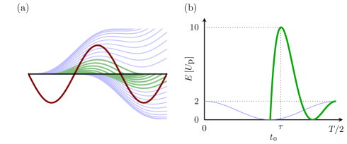
Figure 3: In (a), the classical paths of electrons ionized during one cycle of a laser field, shown in red, is displayed. Analogously to figure 1, the green paths lead back to the core, giving a possibility of rescattering, whereas the blue ensure direct ionization. In (b), the energy $E$ of the directly ionized electrons is shown in blue, and the maximum classical energy of the rescattered electrons is shown in green, both as a function of the ionization time, $t_{0}$, over one half cycle of the field. Classically, electrons can only gain energies of $10U_{\textrm{p}}$ if they are ionized at time $\tau$.

2 Numerical computations

The calculations were done using a newly developed version of the code described in [23], designed to run on graphical processing units. It solves the time-dependent Schrödinger equation in the single active electron approximation and a combined basis consisting of a radial grid and spherical harmonics.

Figure 4: An illustration of how the pulses are simulated. The trapezoidal envelopes for the high- and low-frequency pulses are shown in dark blue and red, respectively. The relative intensity is exaggerated for illustrative purposes. In light red, the low-frequency pulse is shown; in light blue, the high-frequency pulse is shown as a continuous line for $\phi=0$ and as a dashed line for $\phi=\frac{\pi}{4}$.

The pulses were modeled using trapezoidal pulse envelopes. This is advantageous as the asymmetry due to the frequency mixing is present during a majority of the simulated pulse. To study the asymmetry for different $\phi$, the CEP of the high-frequency wave was varied between pulses. Due to the relatively low intensity of the high-frequency pulse, changes to the asymmetry due to boundary effects caused by changing CEP are relatively small. The simulated pulse is illustrated in figure 4.

3 Theory

3.1 Asymmetry as a basis for phase metrology

The force, $\bi{F}$, on an electron in a two-colour laser field can for non-relativistic velocities be approximated as

$$\bi{F}=-q\bi{E}_{\omega}\left[\sin\left(\omega t\right)+\sqrt{I_{\textrm{rel}}}\sin\left(2\omega t+\phi\right)\right],$$ (4)

where $\bi{E}_{\omega}$ is the envelope of the driving field, $I_{\textrm{rel}}$ the relative intensity of the second harmonic, $q$ the elementary charge, $\omega$ the driving field frequency. The carrier waves are shown for four different values of $\phi$ in figure 2.

In figure 5 a schematic ATI spectrum is shown in red. In the monochromatic case, there would be an approximate symmetry between the directions of the field. The addition of the second harmonic, however, breaks that symmetry.

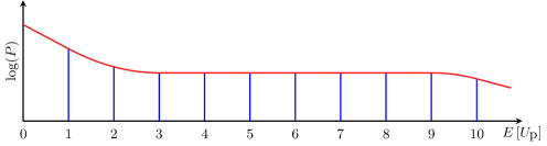
Figure 5: A simplified version of the general characteristics of an ATI spectrum is shown in red, and a division of $\left[0,10U_{\textrm{p}}\right]$ into ten sections, is shown in blue.

The energy of the electrons depend on when during the half-cycle of the field they are ionized, as shown in the right of figure 3. This means that the energy distribution of electrons in the positive direction of the field, $P_{+}\left(E\right)$, will be different from that in the negative direction of the field, $P_{-}\left(E\right)$.

If $\sin\left(\omega t\right)$ and $\sin\left(2\omega t+\phi\right)$ constructively interfere at $t=t^{\prime}$  they interfere destructively at $t=t^{\prime}+\pi$. This is shown in figure 2. As a result, the parts of the sub-half cycle when the driving field is positive, for which there is constructive interference, are the same parts of the sub-half cycle when the driving field is negative, for which the interference is destructive, and vice versa. This will in turn mean that an overrepresentation, due to constructive interference, of electrons with energy $E$ in one direction of the field will coincide with an underrepresentation, due to destructive interference, in the other.

In order to gain information about $\phi$, the asymmetry between $P_{+}\left(E\right)$ and $P_{-}\left(E\right)$ can be studied. Analogously with [18] and [17], the asymmetry of two energy ranges, $\varepsilon_{\mathrm{l}}$ and $\varepsilon_{\mathrm{h}}$, of the ATI spectrum will be studied in this paper. The subscripts $\mathrm{l}$ and $\mathrm{h}$ will below be used to differentiate between the low and the high energy range.

To provide metrics for the respective asymmetries of $\varepsilon_{\mathrm{l}}$ and $\varepsilon_{\mathrm{h}}$, $A_{\mathrm{l}}=A\left(\varepsilon_{\mathrm{l}}\right)$ and $A_{\mathrm{h}}=A\left(\varepsilon_{\mathrm{h}}\right)$ were used, where

$$A\left(\varepsilon\right)=\frac{\displaystyle\int_{\varepsilon}\mathrm{d}E\left[P_{+}\left(E\right)-P_{-}\left(E\right)\right]}{\displaystyle\int_{\varepsilon}\mathrm{d}E\left[P_{+}\left(E\right)+P_{-}\left(E\right)\right]}$$ (5)

is the asymmetry over an energy interval $\varepsilon$ of the ATI spectrum.

For different values of $\phi$, a two-colour pulse can be represented in the $A_{\mathrm{l}}$–$A_{\mathrm{h}}$ plane. Figure 6(a) illustrates this for a hypothetical wave and $\phi\in\left\{0,\frac{\pi}{3},\frac{2\pi}{3}\right\}$. As can be seen in figure 2, changing the value of $\phi$ by $\pi$ completely inverts the asymmetry coming from the second harmonic. Because of this, figure 6(a) can be extrapolated to give the values in figure 6(b).

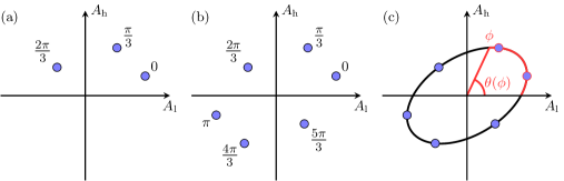
Figure 6: An illustration of the $A_{\mathrm{l}}$–$A_{\mathrm{h}}$ plane. In (a), the representation of a two-colour pulse has been given for $\phi\in\left\{0,\frac{\pi}{2},\frac{2\pi}{3}\right\}$. In (b), an extrapolation of the values in (a) based on symmetry can be seen. In (c), the $\phi$-dependent angle $\theta$ is shown.

Denote the angular coordinate in the $A_{\mathrm{l}}$–$A_{\mathrm{h}}$ plane $\theta$. As is shown in figure 6(c), there exists for certain $A_{\mathrm{l}}$–$A_{\mathrm{h}}$ representations a bijective mapping between $\phi$ and $\theta$. By choosing $\varepsilon_{\mathrm{l}}$ and $\varepsilon_{\mathrm{h}}$ that result in such a mapping, it is possible to gain a measure of $\phi$.

It interesting to note that neither $\phi\rightarrow A_{\mathrm{l}}$ or $\phi\rightarrow A_{\mathrm{h}}$ are injective, which can easily be seen in figure 6(c). As injectivity is a requirement for inversion, it would not be possible to determine a non-ambiguous measure of $\phi$ by observing the asymmetry of a single range of the ATI spectrum, which justifies the previous selection of two energy ranges.

3.2 Measurement of the absolute phase difference

The second harmonic gives rise to constructive and destructive interference during predetermined parts of each cycle. During experiments it is important to be certain of which data point in the $A_{\mathrm{l}}$–$A_{\mathrm{h}}$ plane corresponds to which $\phi$. However, even if the values of $\theta$ in the mapping

$$\theta\left(\phi\right)\in\left\{\theta\left(\phi_{0}\right),\theta\left(\phi_{0}+\frac{2\pi}{N}\right),\cdots,\theta\left(\phi_{0}-\left(N-1\right)\frac{2\pi}{N}\right)\right\}$$ (6)

have been ascertained for given $\varepsilon_{\mathrm{l}}$ and $\varepsilon_{\mathrm{h}}$ by changing $\phi$ in increments of $\frac{2\pi}{N}$, it can be risky to speculate on the value of $\phi_{0}$.

One solution to this problem is found in the right hand side of figure 3, which shows that there is only one ionization time per half-cycle, here called $\tau$, for which electrons can classically obtain energies as high as $10U_{\textrm{p}}$. Due to quantum mechanical effects, it is possible for electrons with other ionization times to obtain equally high energies, but the probability of doing so is small for ionization times which notably differ from $\tau$. Because of this, the highest asymmetry near $10U_{\textrm{p}}$ is observed when the peak of the second harmonic occur at $\tau$. In other words, for some small $\delta$, $A\left(\left[10U_{\textrm{p}}-\delta,10U_{\textrm{p}}+\delta\right]\right)$ will be maximized and positive when the peak of the second harmonic in the positive field direction occurs at $\tau$. The peak of the second harmonic occurring at $\tau+\pi$, on the other hand, maximizes $-A\left(\left[10U_{\textrm{p}}-\delta,10U_{\textrm{p}}+\delta\right]\right)$ .

3.3 Selection of $\varepsilon_{\mathrm{l}}$ and $\varepsilon_{\mathrm{h}}$

Because the asymmetries of $\varepsilon_{\mathrm{l}}$ and $\varepsilon_{\mathrm{h}}$ are measured to determine $\phi$, it is important how the ATI spectrum is divided — the effect of the second harmonic on $P_{+}(E)$ and $P_{-}(E)$ is not equal for all $E$. To make the selection of $\varepsilon_{\mathrm{l}}$ and $\varepsilon_{\mathrm{h}}$, $\left[0,10U_{\textrm{p}}\right]$ was sectioned into 10 equally spaced sections, as illustrated in figure 5. The energy was cut at $10U_{\textrm{p}}$, because it is the highest energy the electrons can classically obtain [19], as illustrated in figure 3(b).

For every pulse, both $\varepsilon_{\mathrm{l}}$ and $\varepsilon_{\mathrm{h}}$ were generated from one or multiple neighbouring sections. The sections were chosen so that

$$\forall E_{\mathrm{l}}\in\varepsilon_{\mathrm{l}},E_{\mathrm{h}}\in\varepsilon_{\mathrm{h}}:E_{\mathrm{l}}\leq E_{\mathrm{h}}.$$ (7)

A total of 495 $A_{\mathrm{l}}$–$A_{\mathrm{h}}$ representations of the energy spectrum were generated, out of which the most useful ones were manually selected. For more information on how the energy spectrum was divided, see [24].

4 Results

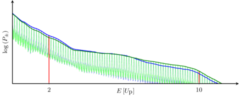
Figure 7: The ATI spectra in the positive and negative directions of a two-colour field, $P_{+}$ and $P_{-}$, shown In blue and green respectively. The peaks of the spectra are outlined in darker colours. The relative intensity of the pulse used to generate the spectrum was $I_{\mathrm{rel}}=0.15$ and the phase difference was $\phi=\frac{\pi}{4}$.

In figure 7 $P_{+}$ and $P_{-}$ for a two-colour pulse are shown. There is an asymmetry between the directions of the field, which can be seen by observing the peaks of the spectra. For almost high energies, $P_{+}$ is dominant, whereas $P_{-}$ dominates for low energies. The asymmetry of electrons with an energy of $10U_{\textrm{p}}$ is largest when the peak of the second harmonic occurs slightly after $\tau$.

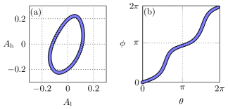
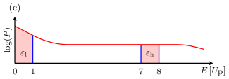
Figure 8: The $A_{\mathrm{l}}$–$A_{\mathrm{h}}$ representation of a two-colour pulse is shown in (a). In (b), the corresponding $\theta$–$\phi$ mapping is shown. The relative intensity was $I_{\mathrm{rel}}=0.01$, and the energy ranges, $\varepsilon_{\mathrm{l}}=\left[0U_{\textrm{p}},U_{\textrm{p}}\right]$ and $\varepsilon_{\mathrm{h}}=\left[7U_{\textrm{p}},8U_{\textrm{p}}\right]$, are shown in (c).

Figure 8(a) shows the $A_{\mathrm{l}}$–$A_{\mathrm{h}}$ representation of a two-colour pulse. In figure 8(b), the $\theta$–$\phi$ mapping can be seen, where $\theta$ is defined as in figure 6(c). For the pulse and energy ranges selected in figure 8,

$$\left.\frac{\mathrm{d}\phi}{\mathrm{d}\theta}\right|_{\theta\in\{0,\pi\}}\ll\left.\frac{\mathrm{d}\phi}{\mathrm{d}\theta}\right|_{\theta\in\{\frac{\pi}{2},\frac{3\pi}{2}\}}.$$ (8)

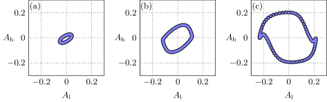
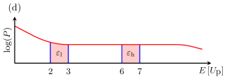
Figure 9: The $A_{\mathrm{l}}$–$A_{\mathrm{h}}$ representations of three two-colour pulses. Between each figure, $I_{\mathrm{rel}}\in\left\{0.001,0.0125,0.15\right\}$ is increased by a factor $\approx 12.5$. In all three figures the energy ranges were $\varepsilon_{\mathrm{l}}=\left[2U_{\textrm{p}},3U_{\textrm{p}}\right]$ and $\varepsilon_{\mathrm{h}}=\left[6U_{\textrm{p}},7U_{\textrm{p}}\right]$, as illustrated below figures (a)–(c).

A problem which might arise due to careless selection of the energy ranges is that $\theta\left(\phi\right)$ stops being bijective. This can be seen in figure 9(c), where neither $\phi\left(0\right)$ nor $\phi\left(\pi\right)$ are unique. This can always be circumvented by proper selection of energy ranges.

As illustrated in figure 9, where $I_{\mathrm{rel}}$ is increased exponentially between figures (a)–(c), the asymmetry increases with $I_{\mathrm{rel}}$. This is to be expected, as the addition of the second harmonic is the cause of the asymmetry, and the radius of the $A_{\mathrm{l}}$–$A_{\mathrm{h}}$ representation can be used to give information about the relative intensity. Note that the $A_{\mathrm{l}}$–$A_{\mathrm{h}}$ representation can change shape as the relative intensity increases. In figure 9(c), the $\theta\left(\phi\right)$ has lost the bijectivity it had for the cases shown in figures 9(a)–(b).

The asymmetry caused by the second harmonic in the two-colour case can be compared to that caused by rapid change of amplitude during few-cycle pulses — changing the CEP affects the asymmetry of the short pulse just as changing $\phi$ affects the asymmetry of the two-colour field. The similarities of two-colour fields to short pulses can be seen in figure 10, where the $A_{\mathrm{l}}$–$A_{\mathrm{h}}$ representation of two short pulses is shown. The pulse shown in figure 10(a) is of half the duration of the one in figure 10(b). It also has significantly higher asymmetry. For short pulses the rapid amplitude change is the cause of the asymmetry. As the amplitude gradient is greater for short pulses, the asymmetry is as well.

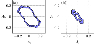
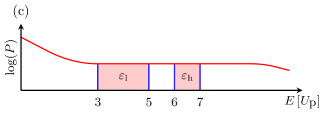
Figure 10: The $A_{\mathrm{l}}$–$A_{\mathrm{h}}$ representations of two short pulses, created by changing the CEP by incements. The pulse used to generate (a) has a Full Width at Half Maximum (FWHM) of 2 field cycles, whereas the one used to generate (b) has a FWHM of 4 field cycles. The different datapoints displayed in figures (a) and (b) were generated by changing the CEP incrementally. The bottom picture shows the studied energy ranges, $\varepsilon_{\mathrm{l}}=\left[3U_{\textrm{p}},5U_{\textrm{p}}\right]$ and $\varepsilon_{\mathrm{l}}=\left[6U_{\textrm{p}},7U_{\textrm{p}}\right]$.

5 Conclusions

By adding the second harmonic to a strong field, it is possible to control the effects it has on matter. To control the effects to an as accurate degree as possible, it is important to know the phase difference, $\phi$, between the two harmonics with good precision. We have shown that it is possible to measure $\phi$ by using Stereo-ATI. The process consists of selecting two ranges of the ATI spectrum and mapping their respective asymmetry to different relative phases. As the asymmetry is caused by the second harmonic, it is also possible to determine the relative intensity of the pulses by measuring the magnitude of the asymmetry.

The second harmonic of a two-colour field can be compared to the rapid change of amplitude of a short pulse. In both cases, the asymmetry of each cycle results in an asymmetrical distribution of ionized electrons. The effect is strengthened by increasing the intensity of the second harmonic and decreasing the pulse width respectively. The asymmetry of the electron distribution can be used to measure $\phi$ and the CEP respectively.

References

- [1] Perry M D and Crane J K 1993 Phys. Rev. A 48 R4051–R4054 URL http://dx.doi.org/10.1103/PhysRevA.48.R4051
- [2] Eichmann H, Egbert A, Nolte S, Momma C, Wellegehausen B, Becker W, Long S and McIver J K 1995 Phys. Rev. A 51 R3414–R3417 URL http://dx.doi.org/10.1103/PhysRevA.51.R3414
- [3] Dudovich N, Smirnova O, Levesque J, Mairesse Y, Ivanov M Y, Villeneuve D M and Corkum P B 2006 Nat Phys 2 781–786 URL http://dx.doi.org/10.1038/nphys434
- [4] Mauritsson J, Dahlström J M, Mansten E and Fordell T 2009 Journal of Physics B: Atomic, Molecular and Optical Physics 42 134003 ISSN 1361–6455 URL http://dx.doi.org/10.1088/0953-4075/42/13/134003
- [5] Nguyen H S, Bandrauk A D and Ullrich C A 2004 Phys. Rev. A 69 ISSN 1094-1622 URL http://dx.doi.org/10.1103/PhysRevA.69.063415
- [6] Brizuela F, Heyl C M, Rudawski P, Kroon D, Rading L, Dahlström J M, Mauritsson J, Johnsson P, Arnold C L and L’Huillier A 2013 Sci. Rep. 3 ISSN 2045-2322 URL http://dx.doi.org/10.1038/srep01410
- [7] Hentschel M, Kienberger R, Spielmann C, Reider G A, Milosevic N, Brabec T, Corkum P, Heinzmann U, Drescher M and Krausz F 2001 Nature 414 509–513 URL http://dx.doi.org/10.1038/35107000
- [8] Reichert J, Holzwarth R, Udem T and Hänsch T 1999 Optics Communications 172 59–68 URL http://dx.doi.org/10.1016/S0030-4018(99)00491-5
- [9] Udem T, Holzwarth R and Hänsch T W 2002 Nature 416 233–237 URL http://dx.doi.org/10.1038/416233a
- [10] Goulielmakis E 2004 Science 305 1267–1269 URL http://dx.doi.org/10.1126/science.1100866
- [11] Brabec T and Krausz F 2000 Reviews of Modern Physics 72 545–591 URL http://dx.doi.org/10.1103/RevModPhys.72.545
- [12] Jones D J 2000 Science 288 635–639 URL http://dx.doi.org/10.1126/science.288.5466.635
- [13] Baltuška A, Udem T, Uiberacker M, Hentschel M, Goulielmakis E, Gohle C, Holzwarth R, Yakovlev V S, Scrinzi A, Hänsch T W and Krausz F 2003 Nature 421 611–615 URL http://dx.doi.org/10.1038/nature01414
- [14] Paulus G G, Grasbon F, Walther H, Villoresi P, Nisoli M, Stagira S, Priori E and De Silvestri S 2001 Nature 414 182–184 ISSN 0028-0836 URL http://dx.doi.org/10.1038/35102520
- [15] Paulus G G, Lindner F, Walther H, Baltuška A, Goulielmakis E, Lezius M and Krausz F 2003 Phys. Rev. Lett. 91 URL http://dx.doi.org/10.1103/PhysRevLett.91.253004
- [16] Mauritsson J, Johnsson P, Gustafsson E, L’Huillier A, Schafer K J and Gaarde M B 2006 Phys. Rev. Lett. 97 URL http://dx.doi.org/10.1103/PhysRevLett.97.013001
- [17] Wittmann T, Horvath B, Helml W, Schätzel M G, Gu X, Cavalieri A L, Paulus G G and Kienberger R 2009 Nat Phys 5 357–362 ISSN 1745-2481 URL http://dx.doi.org/10.1038/nphys1250
- [18] Rathje T, Johnson N G, Möller M, Süßmann F, Adolph D, Kübel M, Kienberger R, Kling M F, Paulus G G and Sayler A M 2012 Journal of Physics B: Atomic, Molecular and Optical Physics 45 074003 ISSN 1361-6455 URL http://dx.doi.org/10.1088/0953-4075/45/7/074003
- [19] Paulus G, Becker W and Walther H 1995 Phys. Rev. A 52 4043–4053 ISSN 1094-1622 URL http://dx.doi.org/10.1103/PhysRevA.52.4043
- [20] Dahlström J M, Fordell T, Mansten E, Ruchon T, Swoboda M, Klünder K, Gisselbrecht M, L’Huillier A and Mauritsson J 2009 Phys. Rev. A 80 ISSN 1094-1622 URL http://dx.doi.org/10.1103/PhysRevA.80.033836
- [21] Dahlström J M, L’Huillier A and Mauritsson J 2011 Journal of Physics B: Atomic, Molecular and Optical Physics 44 095602 ISSN 1361-6455 URL http://dx.doi.org/10.1088/0953-4075/44/9/095602
- [22] Yin Y Y, Chen C, Elliott D S and Smith A V 1992 Physical Review Letters 69 2353–2356 ISSN 0031-9007 URL http://dx.doi.org/10.1103/PhysRevLett.69.2353
- [23] Schafer K J 2009 Numerical Methods in Strong Field Physics vol Strong Field Laser Physics (Springer) pp 111–145
- [24] Petersson C L M 2014 Above-Threshold Ionisation with Two-Colour Laser Fields Master’s thesis Lund University URL http://lup.lub.lu.se/student-papers/record/4856377/file/4856382.pdf