Exact Cosmological Solutions in Modified Brans–Dicke Theory
Abstract
In this paper, we obtain exact cosmological vacuum solutions for an extended FLRW homogenous and isotropic Brans-Dicke (BD) universe in five dimensions for all values of the curvature index. Then, by employing the equations associated to a modified Brans-Dicke theory (MBDT) RFM14 , we construct the physics on a four-dimensional hypersurface. We show that the induced matter obeys the equation of state of a fluid of a barotropic type. We discuss the properties of such an induced matter for some values of the equation of state parameter and analyze in detail their corresponding solutions. To illustrate the cosmological behaviors of the solutions, we contrast our solutions with those present the standard Brans-Dicke theory. We retrieve that, in MBDT scenario, it is impossible to find a physically acceptable solution associated to the negative curvature for both the dust-dominated and radiation-dominated universes. However, for a spatially flat and closed universes, we argue that our obtained solutions are more general than those associated to the standard BD theory and, moreover, they contain a few classes of solutions which have no analog in the BD cosmology. For those particular cases, we further compare the results with those extracted in the context of the induced matter theory (IMT) and general relativity (GR). Furthermore, we discuss in detail the time behaviors of the cosmological quantities and compare them with recent observational data. We find a favorable range for the deceleration parameter associated to a matter-dominated spatially flat universe (for the late times) which is compatible with recent corresponding observational results.
pacs:
04.50.-h; 04.50.Kd; 98.80.-k; 98.80.JkI Introduction
The scalar-tensor theories (for a complete review for applications in cosmology, see, e.g., Faraoni.book ) have been proposed based on the main idea which asserts that the gravitational coupling is time-dependent, an idea related to the large number hypothesis by Dirac D37 ; D38 . He suggested that the gravitational constant decreases with the age of the universe, an assumption that can be in agreement with a few consideration of geological facts J55 ; J66 . Then, the Dirac’s idea has been developed by other physicists by constructing new versions of the scalar-tensor theories in which the gravitational constant has been replaced by a scalar field J48 ; T48 , and consequently it must satisfy a generalized conservation law proposed in the theory. In 1961, the simplest version of the scalar tensor theories was proposed by Brans and Dicke primarily motivated by cosmology and the Mach’s principle BD61 .
Using different methods, exact cosmological solutions have been obtained for the isotropic FLRW models, the anisotropic Bianchi types I-IX and the related Kantowski-Sachs models by assuming various kinds of the ordinary matter in the context of the BD theory (see, e.g., o'hanlon-tupper-72 ; DO71 ; DO72a ; DO72b ; LP-rev ; M78 ; C83 ; CN91 ; BP97 ; qiang2005 ; qiang2009 ; Faraoni.book ; RFK11 ; LF15 and references therein).
Recently, it has been shown that by applying a specific reductional procedure for the conventional BD theory in -dimensional space-time, a MBDT in dimensions is obtained RFM14 . The MBDT has four sets of field equations, in which two sets of them, regardless of the geometrical origin of the matter and scalar potential, are mathematically similar to those derived from the BD standard action with a scalar potential. One set of the mentioned MBDT field equations is the extended version of the conservation equation introduced in induced matter theory (IMT), see e.g., PW92 ; stm99 ; DRJ09 ; RJ10 . Finally, the forth equation retrieved in MBDT has no analog in the conventional BD theory as well as in scalar tensor theories.
To gain an insight into the physical features of the MBDT and comparing the properties of its geometrically induced matter and scalar potential with the ordinary ones assumed in the context of the BD theory as well as with observational data, several investigations have been presented by considering both the spatially flat FLRW universe (in four Ponce1 ; Ponce2 and arbitrary RFM14 dimensions) and the Bianchi type I cosmology RFS11 . We should note that, up to our knowledge, the solutions of the non-flat FLRW space-time have not been obtained in either the higher-dimensional BD theory or the MBDT scenario. Moreover, the herein solutions associated to flat space are wider than the ones obtained in RFM14 . It is important to note that the induced scalar potential and matter in the MBDT lead us to an accelerating universe in late times (as it will be seen in this work) and we do not require to add a scalar potential by hand such as some phenomenological scenarios in the context of the DB theory BP01 ; SS01 .
The aim of this paper will be to employ the MBDT to reduce the five-dimensional FLRW solutions (for all values of the curvature) on a suitably projected four-dimensional space time. We will show that the induced matter obeys the barotropic equation of state and consequently this geometrically originated matter can be examined for particular choices of well-know matter types in the universe. Subsequently, the properties of obtained extended solutions will be analyzed and then they will be compared with the ones obtained from the four dimensional BD theory (with or without a scalar potential) as well as with observational data. We will further show that all the solutions can be considered as the generalized versions of the well-known solutions of the BD theory (e.g., the Dehnen-Obregon, Nariai, O’Hanlon-Tupper solutions) in four dimensional space-time.
In this work, the expressions for physical quantities will be obtained neither by using the conformal time nor by defining other variables to explain the behavior of the scale factor and scalar field, but instead, we will discuss the behaviors from their corresponding direct physical expressions.
Our work is organized as follows. In section II, we review the MBDT set up. In section III, by assuming a five-dimensional FLRW universe (with all values of the curvature), we solve the field equations associated to the standard BD theory in vacuum. In section IV, by means of the MBDT setting, we construct the physics on a four-dimensional hypersurface. We show that the induced matter obeys the barotropic equation of state and consequently it can play the role of either the ordinary matter or dark matter-dark energy in the universe. By assuming a few known values for the equation of state parameter, we discuss the properties of the solutions and compare them with those obtained in the context of the BD theory as well as with observational data. Finally, in section V, we review the main results and add some new discussions.
II Modified Brans–Dicke Theory in Four Dimensions
In analogy to the four-dimensional standard BD theory, the action associated to a five-dimensional BD theory, in the Jordan frame, can be written as
| (1) |
where the Latin indices run from zero to four, is the determinant of the metric associated to a five-dimensional space-time, is the curvature scalar and stands for the covariant derivative in the five-dimensional space-time. Moreover, is the BD scalar field, is the adjustable dimensionless BD coupling parameter and we have chosen . In addition, is the Lagrangian density associated to the ordinary matter which is minimally coupled to the BD scalar field.
The field equations, derived from the action (1), are given by
| (2) |
and
| (3) |
where and is the energy–momentum tensor (EMT) of the ordinary matter fields in a five-dimensional space–time and .
By means of the reduction procedure for the BD theory, the field equations associated to the four-dimensional MBDT can be obtained on a hypersurface. In these field equations, geometrically induced terms will play the role of the ordinary matter sources and scalar potential in an extended version of the standard BD theory111In the Lagrangian density associated to the original BD theory, there is no scalar potential.. Let us be more precise. By applying the well-known line element222The Greek indices run from zero to and stands for the non–compact coordinate associated to fifth dimension. The indicator is chosen such that the extra dimension to be either time–like or space–like, and is another scalar field. stm99
| (4) |
the BD field equations (2) and (3) are induced on the hypersurface ), which is orthogonal to the unit vector where . In this respect, the MBDT, which can be regarded as a generalized version of the IMT, BD theory or GR, conveys four field equations. One pair of these equations reproduces conventional four-dimensional BD field equations but with the specificity that an induced scalar potential is present, in which the induced EMT and the mentioned scalar potential have a geometrical origin. The other pair has no analog in the standard four-dimensional BD theory (for a more detailed presentation of the MBDT, see RFM14 ). We will now explain how our equations for a four-dimensional universe is obtained from a five-dimensional BD setting, on a four-dimensional hypersurface, directly and explicitly computing all terms, by means of dimensional reduction and projection, i.e., all elements having a direct geometric origin, computed consistently and none taken as an ad-hoc assumption. Namely, in the next section, we will use
| (6) | |||||
| (7) |
where is the covariant derivative on the hypersurface and
| (8) |
where and
| (9) |
is the effective matter obtained from the five-dimensional EMT and
| (10) |
is an induced EMT on a four-dimensional space-time in which
| (12) | |||||
| (13) |
where a prime denotes a derivative with respect to the fifth coordinate, . The quantity is an induced scalar potential on the hypersurface which is obtained from
The first term of the induced EMT, i.e. , which bears a resemblance to the one introduced in IMT PW92 ; stm99 , is the fifth part of the metric (4) which is geometrically induced on the hypersurface. Whereas the -part, i.e., , is composed of the BD scalar field and its derivatives with respect to the fifth coordinate, has no analogue in IMT. Moreover, the induced scalar potential is provided completely from the geometry of the fifth dimension rather than adding an extra term by hand, such as the ones usually employed in phenomenological applications of the scalar tensor theories in astrophysics/cosmology see, e.g., SS01 and references therein.
In section IV, we will use these geometrical intrinsic as well as elegant advantages of the MBDT to retrieve BD cosmological features on the hypersurface for a homogenous and isotropic Friedmann universe and compare them with the results of conventional BD theory, other scalar-tensor theories and also with observational data.
III exact solutions of Brans–Dicke cosmology in a five-Dimensional space-time
We start with a five-dimensional extended version of the Friedmann-Lemaître-Robertson-Walker (FLRW) universe in which there is no ordinary matter, i.e., . We will find the exact solutions in the five-dimensional space-time and then, in section IV, by applying the set up reviewed in the previous section, we concentrate on the cosmological solutions further MBDT projected on a four-dimensional hypersuface.
Let us to work with a metric whose components depend only on comoving time. Thus, we consider the line element
| (15) |
where, without loss of generality, we can set the spatial curvature constant as , which correspond to open, flat and closed universes, respectively; are the coordinates associated to a four-dimensional space-time whose spatial sections are spherical symmetric. The and are cosmological scale factors.
Employing equations (2) and (3) with the line-element (15) gives us the dynamical field equations in a five-dimensional space-time, namely
| (16) | |||||
| (17) | |||||
| (18) | |||||
| (19) |
An overdot denotes the derivative with respect to the cosmic time and we have assumed the BD scalar field to depend only on the cosmic time. Equation (16) has been derived from (3), and equations (17), (18) and (19) have been, respectively, obtained by setting , and into Eq. (2).
We should note that the coupled non-linear equations (16)-(19) are not independent. To solve these equations, let us consider a well-known assumption: we employ Dirac’s hypothesis that states the gravitational constant and the scale factor of the universe should be related to each other by a power law relation DO71 ; DO72a ; DO72b . As in the BD theory the scalar field is proportional to the inverse of the gravitational constant [see Eqs. (48) and (49)], we can write
| (20) |
In order to get consistent solutions, the above assumption leads us to consider also a power law between and , as
| (21) |
In relations (20) and (21), (corresponding to attractive gravity) and are constants which are not independent and they can be determined in an arbitrary fixed time; and are parameters which must satisfy the field equations333From current particle physics data, it can be assumed that for an extra coordinate having lengthlike nature, it must be very small at the present time KS91 ; OW97 , i.e., it must contract with time. However, in this paper, to get a comprehensive list of solutions, we will also investigate the cases in which . (16)-(19).
From (16), after a simple integration, we get
| (22) |
where is a constant; plugging and from (20) and (21) into (22), we obtain
| (23) |
where and we have assumed that at the initial time , the scale factor vanishes. By employing the power-law solutions (20) and (21) in (17), we obtain
| (24) |
In what follows, we will investigate all the possible solutions associated to the flat space () and non-flat spaces ().
III.1 Flat Space Solutions
For the flat space, by substituting into (24), we obtain the following algebraic equation
| (25) |
Equation (25) gives in terms of as
| (26) |
Thus, the general solutions for the flat space are given by relations (20), (21) and (23) in which and are not independent and they are related according to (26). These solutions are classified into two sets: (i) the power-law solution when , in which and are not independent and they are related to each other by (26); (ii) the exponential solution that is obtained when . To retrieve the second class of solutions, we have to start from the field equations (16)-(19). It is straightforward to show that
| (27) |
where is an integration constant. For this particular case, from (25), in terms of the BD coupling parameter is given by
| (28) |
where, when , for the upper case (plus sign) goes to unity while
for the lower sign, it goes to minus infinity. Namely, for the
former we get a contracting fifth dimension with time, while for the latter the fifth dimension increases by time.
III.2 Non-Flat Space Solutions
For , by employing (23) into (24) we get an algebraic relation which is satisfied for all values of provided that
| (29) |
Thus, from (23) the general solutions associated to the non-flat space can be briefly summarized as
| (30) |
where
| (31) |
Besides, by employing relations (19), (29), (30) and (31), it is easy to show that
| (32) |
where in the particular case , and consequently the BD scalar field takes a constant value. In this case, we cannot find a finite value for the scale factor . Namely, in this case, when there is no vacuum solution. As when the BD coupling parameter goes to infinity, the BD theory may reduce to GR, thus the above result is in agreement with the fact that there is no vacuum solutions associated to the FLRW universe in GR (without a cosmological constant term) for .
In the special case where the scalar factor of the fifth dimension is a constant, i.e., , by setting , equation (31) gives
| (33) |
Therefore, for the cases with the positive curvature () and negative curvature (), we must choose and , respectively. From (33), for both of these cases, we get , and thus by substituting this relation into (30), we obtain
| (34) |
IV Effective Brans-Dicke cosmology on a four dimensional hypersurface
In this section, we will employ the MBDT set up reviewed in section II, for the obtained solutions of the previous section to construct the physics on a four-dimensional space-time. Then, we evaluate the properties of the corresponding solutions and compare them with those of the standard BD theory.
The non-vanishing components of the induced matter on the hypersuface can be obtained by substituting the components of the metric (15) and the isotropic BD scalar field in relation (10), as
| (35) | |||||
| (36) |
where (with no sum) and the induced potential will be derived using the differential equation (II). From (36), it is clear that the different components of are equal, thus the induced matter can be considered as a perfect fluid.
The induced scalar potential is evaluated on the four-dimensional hypersurface by substituting the solutions (20), (21), (23) and (30) into (II). Thus, we obtain444We should notice that some quantities appearing in different solutions have different values. For instance, the quantity , which is seen in the upper and lower relations of the induced scalar potential (37), has different values in terms of the corresponding parameters; such that this quantity for the non-flat space is related to the other quantities by (31); whereas we have not obtained any general relation for this quantity in the case of the flat space.
| (37) |
For a non-flat space, integrating the lower differential equation of (37), by assuming that the constants of integration are zero, we get
| (38) |
where , according to relation (31), is a function of the parameters , and the curvature constant .
From the upper equation of (37), the power-law scalar potential associated to the flat space is given by
| (39) |
where we have set the integration constant equal to zero.
The power-law scalar potential555As the logarithmic effective potential leads to inconsistency for applying the energy conditions, we opt to abandon the solutions associated to this case of the induced scalar potential. [i.e., the lower relation in (38) for non-flat space and (39) for flat space, whose solutions, in what follows, will be discussed in this paper], vanishes in the particular cases where either666In the special case where , the BD theory corresponds to the low energy limit of the bosonic string theory. Moreover, in this case, scalar-tensor theories contain certain similarities with supergravity and string theory M86 ; Faraoni.book . or .
For the power-law scalar potential, by employing (23) and (30) for flat and non-flat spaces, we obtain the induced scalar potential versus cosmic time as
| (40) |
In order to write the components of the induced matter (associated to the power-law cases) on the hypersurface, we employ (20), (21), (23), (31), (30), (40), and relations (35) and (36). Thus, the energy density and the isotropic pressures for the non-flat and flat spaces are given, respectively, by
| (41) |
where
| (42) | |||||
| (43) |
and (for the flat space)
| (44) | |||||
| (45) |
The above geometrical effective matter relations give a barotropic equation of state associated to an induced perfect fluid for all the cases. Namely
| (46) |
where
| (47) |
By using the relations (23), (32), (46) and (47), it is straightforward to show that the induced matter (on the four-dimensional hypersurface) is conserved, namely . This result is of relevance in the context of scalar tensor theories, because it allows us to state that the BD scalar field does couple minimally with the induced matter and thus, the herein model does respect the Principle of the Equivalence.
As we would like to study, in particular, the behavior of the gravitational coupling, we review herewith general features associated to it. As the field equations (6) corresponds to the conventional BD field equations, the Newton’s gravitational constant (in a four-dimensional space-time) can be read Faraoni.book
| (48) |
Moreover, we should note that the above definition has been used in cosmological application, rather than in the analysis in the context of the Post-Newtonian formalism W06 , where the relation
| (49) |
has been defined for spherically symmetric solutions N68 ; Faraoni.book ; EP01 ; NP07 and employed the Solar System experiments. However, we should note that the rate of variation of and have the same features.
In what follows, we will elaborate on the MBDT above retrieved for concrete values of the equation of state parameter. After probing the properties of the geometrical induced matter, we compare the results with those obtained from the conventional BD theory and observational data.
IV.1 Vacuum Cosmologies
One of the main questions in the context of scalar-tensor theories is whether non-trivial vacuum (absence of ordinary matter) solutions exist or not. Such solutions are very interesting because when asymptotically tends to zero, the fluid-filled FLRW solutions approach the vacuum solutions for wide ranges of the varying BD coupling parameter B93 . After the seminal papers by Brans and Dicke, to our knowledge, this question has been investigated by O’Hanlon and Tupper o'hanlon-tupper-72 . They found the cosmological non-static vacuum solutions for the BD theory for spatially flat FLRW metric and addressed questions such as the validity of the Mach’s principle and Birkhoff theorem in the BD theory. However, for the non-flat FLRW space, they only found solutions for spacial values of the BD coupling parameter, . Subsequently, the whole class of solutions associated to the latter (non-flat) case have been obtained by Dehnen and Obregón by assuming a power law relation between the scale factor and the effective gravitational constant DO72b .
In what follows, we investigate the simple case in which there are not any effects of the geometrical induced matter and scalar potential on the MBDT four-dimensional universe. In this case, we expect to get solutions which would be similar to those obtained in the context of the conventional BD theory for a four-dimensional FLRW universe.777For convenience, from now on, we will investigate the solutions associated to the flat and non-flat spaces in separated parts.
IV.1.1 Flat space
For the flat space () and non-flat spaces () the only manner to get the vacuum cosmology on the hypersurface is setting . Therefore, for the first class of solutions (power-law solutions), by substituting into the solutions associated to the flat space [i.e., relations (20), (21) and (23) in which and are related to each other by (26)], after calculations, we get
| (50) | |||||
| (51) |
where we have assumed and (or ). For this case, from (37), without loss of generality, we can set the induced scalar potential equal to zero, and thus, from using relations (35) and (36), we find that the induced matter also vanishes on the hypersurface. The relations (50) and (51) correspond to the well-known O’Hanlon and Tupper solution o'hanlon-tupper-72 ; RM14 which has been obtained for a four-dimensional spatially flat FRW universe in the standard BD theory where the ordinary matter is absent. Let us present the above solutions in terms of Hubble parameter , and the age of the universe, . From (50), we get
| (52) |
Therefore, relations (50) and (51) can be written as
| (53) | |||||
| (54) |
where from the present values of the scale factor, Hubble constant and scalar field (i.e., , and , ), we can determine the constant .
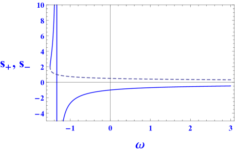
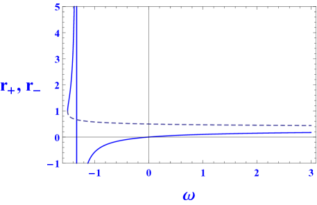
Let us now discuss the behavior of the gravitational coupling, according to relation (54), when and . In888It will be of interest to discuss, for reason of convenience, the behavior of these and other quantities by the least possible number of figures. However, unfortunately, as we will see, for some cases, because of different ranges and scales used, it is not a feasible task. Fig. 1 (the left panel), we have plotted the behavior of , the power of the cosmic time associated to the gravitational coupling. As it is seen, for either the upper case (plus sign) (only when the BD coupling parameter restricted to ) and lower case (minus sign), the behavior of the gravitational coupling is contrary to Dirac’s hypothesis. Whereas, for the upper case, when the gravitational coupling decreases with cosmic time which is in accordance with Dirac’s hypothesis. Regarding the behavior of the scale factor, we see that only is restricted as , we get , (see Fig. 1, the right panel), namely, which corresponds to an accelerating behavior of the scale factor for the upper case. The scale factor of the universe decelerates when either (for the lower case) or (for the upper case). From (52) for the upper case, we see that when the BD coupling parameter is larger than and approaches to , the value of the age of the universe takes large values.
For the second class (exponential solution), by setting into relations (27) and (28), we find the solutions associated to for the upper case (plus sign) as
| (55) |
whereas that the lower case does not give acceptable solution.
In other words, we have
| (56) |
which indicates that the O’Hanlon and Tupper solution in the limiting case approaches to the de Sitter space, likewise the conventional BD theory, see, e.g., Faraoni.book . Similar to the first class of the flat space with , for this case also the components of the induced matter and the scalar potential vanish. We should note that, similar to the standard BD theory, the solution (56) is the unique de Sitter solution associated to the flat and vacuum space; and it is different from the one obtained in GR with a minimally coupled scalar field, in which that scalar field takes a constant value. By assuming that , from (56), we see that the BD scalar field decreases with cosmic time and thus the effective gravitational coupling (48) increases with time; such a behavior is contrary to Dirac’s hypothesis.
IV.1.2 Non-flat space
It should be noted that there are no vacuum solutions associated to FLRW space with in GR in the absence of the cosmological constant LP83a . However, such solutions have been found in the BD theory CE83 ; C83 ; LP83a . In what follows, we would like to investigate the corresponding solutions in MBDT.
In the case of the non-flat space where , we get and the scale factor and scalar field are given by (34). For this case, from relations (II), (21), (35), and (36), we find that the induced matter and scalar potential vanish on the hypersurface. The cosmology associated to this case is the same as that obtained by Dehnen and Obregón in DO72b . With , the age of the universe at present time999The age of the universe estimated by best fit to the Planck 2013 data Planck2013 has been reported billion years., the solutions (34) can be given by
| (57) |
in which the present values associated to the scale factor and the BD scalar field are
| (58) |
We should note that by determining , and , the solutions associated to the closed and open universes cannot be distinguished if the BD coupling parameter restricted to and , respectively.
IV.2 Dust Cosmologies
Dust solutions associated to the FLRW universe in the context of the BD theory (with vanishing scalar potential) have been investigated in BD61 ; DO71 . In M82 ; M01 , some properties of the mentioned solutions have been discussed for large values of . Furthermore, there are a few publications in which the solutions have been obtained in terms of the conformal time and other variables different from the scale factor and the BD scalar field MW95 ; TV96 ; O97 ; Faraoni.book .
IV.2.1 flat space
For this case, by solving equations (47) (upper case) with together with the general equation (25) associated to the flat space, we obtain two classes of solutions as
| (59) |
Thus, by substituting the above values for and into (20), (23), first relation of (40) and (43) the solutions associated to the flat space are given by
| (60) | |||||
| (61) | |||||
| (62) | |||||
| (63) |
where
| (64) | |||||
| (65) | |||||
| (66) | |||||
| (67) |
where , and the parameters and are related to each other as . For this case, the scale factor of the fifth dimension is given by
| (68) |
As , , and must take positive values for an arbitrary fixed time, therefore, we can find the allowed ranges for the BD coupling parameter for these solutions. We should note that to have reasonable solutions, and must take positive values, but can take either positive or negative values, each of which gives two classes of solutions, one for the upper case and another for the lower case. Let us categorize the resulted solutions in terms of the sign of .
- Case I; :
-
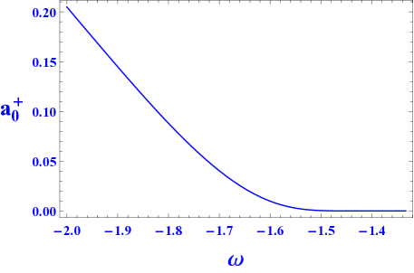
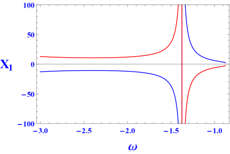
For the lower case (minus sign), as the induced energy density and the scale factor do not take real values in an arbitrary fixed time, thus we abstain from considering them as acceptable solutions. However, for the upper case (plus sign), when the BD coupling parameter restricted to , we found that , , and take positive real values (see Fig.2) and consequently this case can be a physical solution. In this setting, we see that for the allowed values of , , i.e., we get an accelerating universe. In addition, which means that the BD coupling parameter decreases with the cosmic time. Namely, the gravitational coupling increases with time which is not in agreement with Dirac’s hypothesis. Moreover, the induced energy density and the fifth dimension decrease with time.
- Case II; :
-
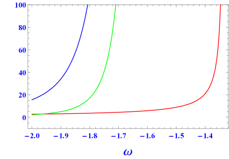
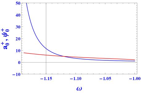
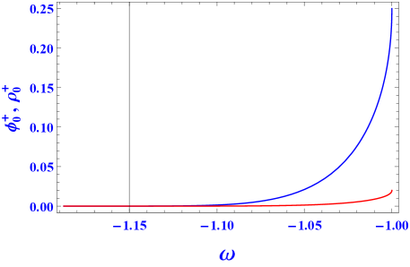
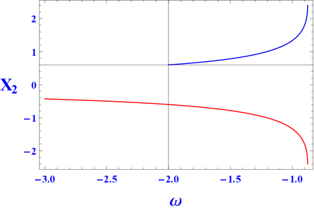
For the lower case (minus sign) the quantities , , and (in an arbitrary fixed time) take positive real values when the BD coupling parameter is restricted to . Whereas for the upper case (plus sign), we find a narrow range for the BD coupling parameter which gives acceptable solutions. Although in this case, , and (for an arbitrary time) take positive real values when , but as is negative when , therefore the allowed range is in which the solution is acceptable. In Fig. 3, for the corresponding allowed ranges, we have shown the behavior of the mentioned quantities versus for an arbitrary fixed time.
Let us summarize briefly the behavior of the quantities associated to this case for the corresponding allowed ranges: (i) we found that, for the lower case, the scale factor of the universe decelerates with cosmic time while we have a contracting scale factor for the upper case. (ii) Both of and take positive values, namely, the BD scalar field always increases with cosmic time and, consequently, the gravitational coupling decreases with time which is in agreement with Dirac’s hypothesis. (iii) for the lower case, both the induced energy density and the scale factor of the fifth dimension decreases with time. However, for the upper case, the induced energy density increases with time while the fifth dimension contracts with time.
IV.2.2 non-flat space
For this case, by considering the lower equation of (47) and solving , we get two values for which both of them depend only on the BD coupling parameter as
| (69) |
where and . We should note that when tends to ,
and goes to infinity and , respectively.
Replacing and from (69) and (70) into (30), the lower relation of (40) and (41), we get four classes of mathematical solutions as101010Indeed, we have two kinds of solutions specified with (the first solution with and the second solution with ), which they, in turn, have two cases specified as an upper case (plus sign) and a lower case (minus sign).
| (71) |
where
| (72) |
In what follows, we will investigate each case, separately, discussing the acceptable solutions associated to each case.
However, we should point out a few general features which are common to all the solutions.
The first point is that as the quantity appears in all the
solutions, so, for every acceptable solution, the BD coupling parameter must be restricted to .
The second point is that as also appear in relations of ,
thus, to get acceptable solutions, the right hand side of (70) must take positive
real values. As depends on the curvature
index, thus, we have to discuss about its behavior by considering also the sign of .
First solution (): In this case, for the closed
universe, we find that takes positive values when ,
while for the open universe it takes positive values when (see Fig. 4, the left panel).
Therefore, by considering the allowed range from ,
we find that the acceptable range for the closed universe
will be while for the open universe will be .
Second solution ():
For this case, takes positive values when . Moreover, also takes real
values for this range, thus, this range can be acceptable for the
closed universe. However, for the open universe, takes negative values
(see the right panel of Fig. 4), thus, there is no acceptable solution for this case.
Within the above discussion, we identified allowable ranges for .
Now, we can apply these to find solutions associated to the open and closed universes, separately.
-
•
Open Universe:
- First solution:
-
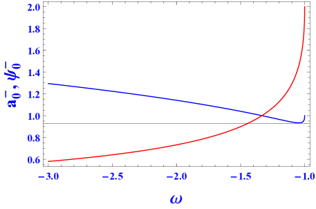
Up to now, in order to have allowable values for and , we found that the BD coupling parameter must be restricted to . However, in this range and must take also positive values. The numerical results show that, in this range, , while , see Fig. 5, the left panel. Namely, the upper solution (plus sign) is not acceptable, while the lower solution (minus sign) can be an acceptable solution provided . But just by looking at the relation of in (72), we find that for this range never takes only real values and it has also imaginary part. In Fig. 5 (the right panel), we have plotted the imaginary part of it. Thus, for this case, there is no physically acceptable solutions.
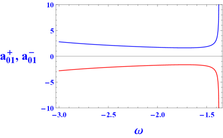
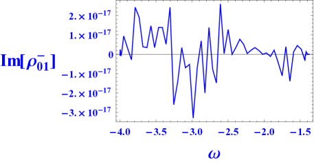
Figure 5: The left and right panels show respectively the behavior of scale factor and the imaginary part of versus . The mentioned quantities are associated to the first solution with which have been plotted in an arbitrary fixed time. In the left panel, the blue and red curves correspond to and , respectively. - Second solution:
-
As mentioned before, , there is not any acceptable solution for this case.
Therefore, the reduced cosmology arisen from the MBDT field equations, for the FLRW open universe which is filled with dust fluid just gives a few mathematical solutions which cannot be physically acceptable solutions.
-
•
Closed Universe:
- First solution:
-
As discussed above, for this case, the allowed range is . Now, we should examine this range to see whether it can generates positive real values for and or not. For the upper case (plus sign), we see that the range gives . We can see that, for this range, . In Fig. 6 (left panel), we have plotted the behavior of and versus . Our numerical results show that, in this allowable range, always takes very small real values which can be physically acceptable. From (72), as and , thus, and . Finally, we conclude that the first solution (upper case) in the range is an acceptable solution for the closed universe.
However, for the lower case, although in the range , we get ; but in this range, does not take real values, thus, we cannot accept this case as a physical solution.
Let us investigate the behavior of the quantities for the upper case in terms of cosmic time. From relations (30), the lower relation of (40) and (41), we see that increases versus time, linearly; the behavior of , and versus the allowable determines the behavior of the quantities associated to this case. For , we find that and take positive real values, whilst always takes negative values. Namely, and increase versus time, while decreases versus time. As the fifth dimension contracts with the cosmic time, it is favorable. Moreover, as the BD coupling parameter increases versus time, thus the gravitational coupling decreases with time which is in agreement with the Dirac’s hypothesis.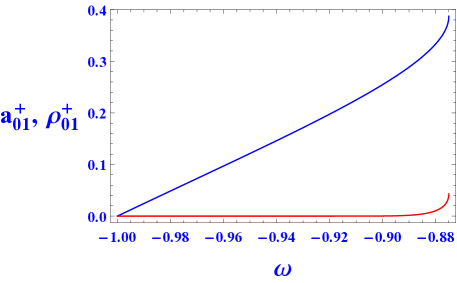

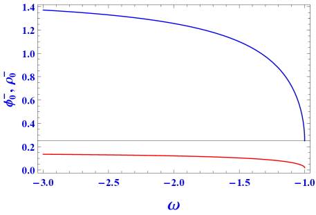
Figure 6: Left panel:the behavior of the scale factor (the blue curve) and induced energy density (the red curve) versus in an arbitrary fixed time associated to the first solution (upper case) and . Note that, regardless of the left panel, our other numerical endeavors show that at the mentioned allowed range of takes very small values which are nonzero. Right panel: the behavior of (the blue solid curve), (the blue dashed curve) and (the red curve) versus associated to the second solution for the closed universe. - Second solution:
-
For this case by considering the allowable values for and , we obtained the allowable range111111We should note that as when , goes to infinity, thus we exclude the value from this solution. . Let us prob this range and investigate if positive real values for the scale factor and the induced energy density in an arbitrary fixed time can be obtained. From (72), for , we find that while , see the right panel of Fig. 6. Namely, the lower case does not give acceptable solution. Now, we should determine the behavior of the induced energy density for the upper case. By means of numerical methods, it is straightforward to show that takes positive real values in the allowable range, see the right panel of Fig. 6.
As we have shown that the second solution (upper case) is an acceptable solution, determining the behavior of the quantities versus time will be a worthwhile task. Similar to the previous case, increases linearly with time; and the behavior of , and versus determines the behavior of the other quantities versus time. We can easily show that for , takes negative values, while for , it takes positive values. Namely, for the former range the induced energy density decreases by time, whereas for the latter range it increases with time. However, for all the values which are taken from () produces positive real values which leads to an increasing BD scalar field by the cosmic time. Thus, the gravitational coupling decreases with time which is again in agreement with the Dirac’s hypothesis. Finally, as always takes positive values, thus the fifth dimension contracts by the cosmic time.
IV.3 Radiation Cosmologies
Radiation dominated universe in the context of the standard BD theory has been investigated in RF76 ; LP-rev ; SD89 ; XY93 ; BP97 . In what follows, we will find the specific solutions associated to radiation-dominated universe in MBDT and discuss the properties of corresponding quantities and their differences with those obtained from standard BD theory.
IV.3.1 Flat Space
By setting in the upper relation of (47) and solving this equation together with the one obtained for the flat space in 5D, i.e., equation (25), we get121212The other solution is , in which the BD scalar field takes constant value. To find the exact solution for this case, we must start from equations (16)-(19). Solving them by assuming a power-law for the scale factor gives and (where and are constants), which is the unique solution of the Einstein field equations in vacuum for the spatially flat FLRW metric in a five-dimensional space-time.
| (73) |
By substituting the above values of and into relations (20), (21), (23), as well as the upper relation of (40) and (44), we get the following solutions
| (74) |
where the constants , , , and are given by
| (75) | |||||
| (76) | |||||
| (77) | |||||
| (78) |
where the constants , and can be determined by knowing the age of the universe and its energy density at the present time. The scale factor of the fifth dimension is given by
| (79) |
Let us first find the allowable ranges of for this case. As , , and should take positive real values, from relations (75) and (78), we find that the allowed ranges of the BD coupling parameter, which depends on the sign of . Therefore, in what follows, we would investigate two separated solutions.
- Case I; :
-
In this case, when the BD coupling parameter is restricted to , the quantities , and take positive real values whereas takes positive real values when . Therefore, the allowed range for this case is ; see the upper panels of Fig. 7. For this allowed range, it is straightforward to show that . More precisely, the scale factor of the universe decelerates with cosmic time. Furthermore, the induced energy density, BD scalar field and the fifth dimension decrease with time.
- Case II; :
-
In this case, to get positive real values for the corresponding quantities (in an arbitrary fixed time), must be restricted to (see the lower panels of Fig. 7), which gives reasonable results for the radiation-dominated universe as follows. It is easy to show that (i) for , we get , while for , we get . The former range (of the power of the cosmic time associated to the scale factor) leads us to a spatially flat universe whose scale factor contracts with the cosmic time; whereas the latter leads to a decelerating universe. (ii) the energy density increases with the cosmic time for whereas it decreases with time when . (iii) the BD scalar field increases with the cosmic time; in this case the gravitational coupling decreases with time which is in agreement with Dirac’s hypothesis. (iv) also decreases with cosmic time for all allowed values of . The above properties imply that the MBDT scenario, by assuming the mentioned constraint on the BD coupling parameter, can be a relevant model for getting a radiation-dominated universe when , in which the induced matter can play properly the role of ordinary matter in the universe.
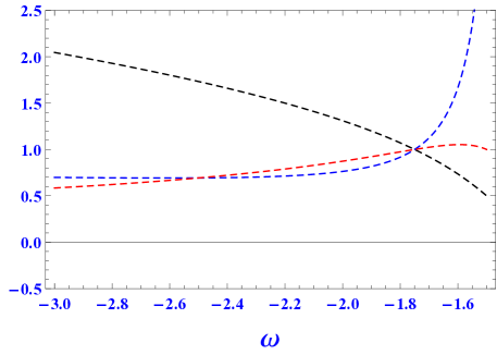
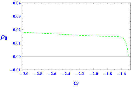
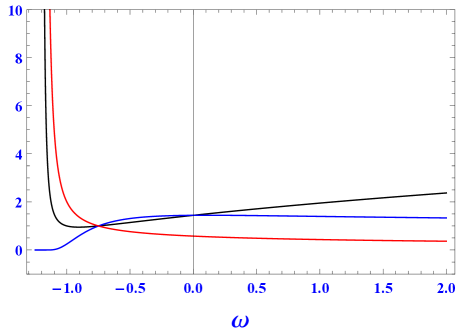
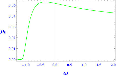
Figure 7: The behavior of (black curves), (the blue curves), (the red curves) and (the green curves) versus (in an arbitrary fixed time) for the spatially flat FLRW universe which is filled with radiation. The dashed and solid curves are associated to and , respectively. We have chosen the constants as and in agreement with the assumptions of cases I and II.
IV.3.2 non-flat space
For this case, by setting in the lower relation of (47), it is easy to show that131313The other solution for this case is , which, according to (30), yields a constant value for the BD scalar field and infinite value for the scale factor. As discussed in section III, in this case the BD theory may reduce to GR and thus such a result is reasonable.
| (80) |
where .
By substituting from (80) into (31), we get
| (81) |
where . By employing relations (80) and (81) for the general solutions associated to the non-flat space, namely (30), we get
| (82) |
where
| (83) | |||||
| (84) | |||||
| (85) | |||||
| (87) |
In what follows, we discuss
the behavior of the quantities for closed and open Universes, separately.
-
•
Open Universe: For this case, by substituting into (83), we find that, in order to get real values for the square root, the BD coupling parameter must be restricted to . On the other hand, must take positive values, thus for the upper case (plus sign) we get , which does not have overlap with the previous allowable range of . Therefore, there is no consistent physical solution for the upper case. However, for the lower case (minus sign), must be restricted to , which has a overlap with the previous allowed range. Namely, in this case, the range not only gives a real values for but also produces positive values for . Nonetheless, this is not enough to have a acceptable physical solution. More concretely, other quantities such as , and must take real positive values in the mentioned range of . However, just by investigating , we find that it takes imaginary values in the mentioned range. Finally, we can conclude that the set of solutions (82) for an open universe are only valid as mathematical solutions, namely, for the FLRW universe with (when and are related to the scale factor with a power-law equation), the MBDT scenario does not yield any physical solution.
-
•
Closed Universe: By substituting into relations (82)-(87) we get two classes of solutions for this case. Let us describe the corresponding quantities for this case by finding the allowable range for the BD coupling parameter. From (83), we see that to have real values for the square root, must be restricted to either or . By considering these allowable ranges of , in what follows, we investigate the solutions associated to the upper case (plus sign) and lower case (minus sign), separately.
- Upper sign:
-
In this case, from (83), we find that takes positive values if the BD coupling parameter is restricted to . For this allowed range of , as and , thus, , and take positive real values for an arbitrary fixed time, see Fig. 8. Consequently, the acceptable physical solutions associated for a closed universe with upper sign (which is filled with radiation) are given by (82) in which must be larger than .
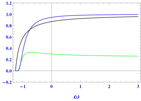
Figure 8: The behavior of (the black curve), (the green curve), (the blue curve) and (the red curve in the left panel) in an arbitrary fixed time versus () associated to the closed universe (and upper sign) which is filled with radiation. We have chosen . Note that and take very small (but nonzero) values when . It is also noteworthy to describe the time behavior of quantities associated to this case. From (82), it is straightforward to show that for , (i) as and , thus, the BD scalar field always increases with the cosmic time; hence, the gravitational coupling decreases by cosmic time which is in agreement with Dirac’s hypothesis; (ii) as , we see that the induced energy density increases with time when , whilst it decreases with time when ; (iii) always decreases with the cosmic time which is a relevant outcome.
- Lower case:
-
For this case, takes positive values when the BD coupling parameter is restricted to either or . However, likewise for the lower case for the open universe, we cannot obtain real values for the energy density in arbitrary fixed time when .
V summary and discussions
The MBDT RFM14 has four sets of field equations: one set corresponds to the generalized version of the conservation law introduced in IMT PW92 ; stm99 . Another set is a nonlinear differential equation associated to the scale factor of the extra dimension which has no analog in the standard BD theory. Finally, the other two sets can be related to the conventional BD action, but with specific scalar potential, in four dimensions in which the matter and the scalar potential have an intrinsic geometrical origin. This induced matter is composed of three parts, see Eq. (10). The first part is a function of the first and second derivatives of the metric components with respect to the extra dimension. The second and third parts are functions of the BD scalar field, metric components and their derivatives with respect to the extra dimension.
Achieving unification of matter and geometry has been claimed as the main motivation for introducing a large extra dimension in IMT Pon01 . As the MBDT can be considered as an extended version of the IMT, thus the motivation that has been followed to also consider a large extra dimension to construct the MBDT scenario. However, in MBDT, in addition to the geometrically induced matter, there is also an induced scalar potential which has also been of interest to discuss in MBDT. This scalar potential has been employed to yield either an accelerating universe Ponce1 ; Ponce2 ; RFM14 (by assuming a spatially flat FLRW universe) or obtaining more general solutions for a Bianchi type I model RFS11 . The main objective of our herein work was to employ the MBDT scenario to obtain new extended solutions associated to both the spatially flat FLRW universe (by assuming more generalized power-law solutions than ones assumed in the previous works) and the non-flat space with respect the corresponding solutions in the context of the conventional BD theory.
In this paper, we started from the geometry of the five-dimensional bulk and then constructed the physics on the projected four-dimensional hypersurface. More precisely, by considering a five dimensional FLRW universe (without ordinary matter) with all values of the curvature index, we have derived the equations of the standard BD theory whose scalar field only depends on the cosmic time. Then, by assuming the Dirac’s hypothesis, which claims that the gravitational constant should be connected to the scale factor of the universe in a power-law relation, we have solved the equations of motion. Our results show that there is a general solution for the non-flat space [see Eqs. (30)] and two kinds of solutions for the flat space, the general power-law solution and exponential solution. We have also discussed regarding some particular cases of theses solutions when either or takes special values.
Subsequently, we have employed the MBDT set up (reviewed in section II) to construct the physics on a four-dimensional space-time. First, we found the relations associated to the induced matter and induced scalar potential in general cases. Our results have shown that the induced scalar potential is in either logarithmic or power-law forms. As the former leads to an inconsistency to apply the energy conditions, we abstained from proceeding to study it. However, the latter yielded the equations of state for the barotropic matter for all values of the curvature index. Such an induced matter, in which all the terms emerge from the geometry of the fifth dimension, has interesting properties. Namely, it obeys the conservation law similar to the ordinary matter in the standard BD theory. Thus, it respects the Principle of Equivalence. Besides, it is worthwhile to emphasize that the induced scalar potential, which contributes to construct the induced matter and consequently the behavior of the BD scalar field, has been induced from the geometry (as a fundamental concept) rather than adding it by hand to the action. As there is a nonzero scalar potential, thus, the relations associated to the scale factor, the BD scalar field and the components of the induced matter, which depend effectively on and/or , are more generalized than those of the conventional BD theory.
We proceeded to study the properties of the induced matter on the hypersurface as consequence of the effects of the geometry of the fifth dimension and contrast it with the ones reported from ordinary matter in the BD theory. For that, we have concentrated on known types of the matter, which, in what follows, we summarize and compare them with those obtained from the conventional BD theory, IMT and GR.
-
1.
Vacuum solutions: For both the flat and non-flat spaces, the only manner to get vacuum solutions on a four dimensional hypersurface is setting , i.e. assuming . In this case, we found that the induced scalar potential and the components of the induced matter vanish. We have shown that the solutions associated to the herein model are similar to those obtained in the standard BD theory. Namely, we obtained the same exact solutions obtained by O’Hanlon-Tupper o'hanlon-tupper-72 and Dehnen-Obregón DO72b in the context of the standard BD theory in vacuum. By means of numerical analysis, we further investigated the time behavior of the scale factor, BD scalar field and the gravitational constant for each solution. We should note that the calculations associated to the vacuum case can be an appropriate procedure to test the correctness of the results produced by the MBDT scenario. For all the solutions associated to the vacuum case, we see that the power-law assumption between the scale factor of the fifth dimension and the BD scalar field as well as the scale factor of the universe, is in contradiction with the Dirac’s hypothesis. The other general consequences of these solutions have shown that, similarly to the conventional BD theory, the Birkhoff theorem and the Mach’s principe, which implies that the matter in the universe determines the value of the gravitational coupling, are not valid in the context of the MBDT.
-
2.
Dust solutions: For a flat space, we found two classes of mathematical solutions [the upper and lower cases, see Eqs. (60)-(63)] which depend on the sign of integration constant . We have discussed the effects of the sign of on the solutions associated to the upper and lower cases. By assuming , we found that only one of the solutions (the upper case) is physically acceptable when . For this case, we have shown that the scale factor of the universe accelerates, while the BD scalar field and induced energy density decrease with cosmic time. Let us compare the result with the observational data: from relations (64), it is straightforward to show that, when then can be restricted as or, equivalently, the deceleration parameter (at present time) is restricted to , which is in agreement with the recent observational measurements Giostri12 .
For , we found that both of the solutions can be physically acceptable. We have also discussed the properties of the quantities for this case. We found that, for both of the upper and lower solutions, the gravitational constant decreases with cosmic time, which is in agreement with Dirac’s hypothesis. It is worthy that for all of the mentioned dust solutions associated to the flat space, the fifth dimension decreases with cosmic time which can be an interesting result in the context of higher dimensional models.
Let us summarize and further discuss solutions (59)-(68) for large values of . For these cases (upper case with and lower case with ), without loss of generality, we can set . As and always take positive values and takes negative and positive values for the former and latter cases, respectively, thus, takes negative and positive values for the former and latter, respectively. From this, it is easy to show that when , we get , , and . Namely, the results are in agreement with those obtained from IMT and thus with GR.
For non-flat space, , we got four different classes of mathematical solutions, see the set of relations (69)-(72). By further probing of the properties of the solutions associated to the open universe, we discovered that there is no physically acceptable solution for it. This result is in accordance with the one obtained for the standard BD theory DO71 .
However, for the closed universe, among four classes of mathematical solutions, we have shown that only two of them can be physically acceptable. In one class of those solutions (the first solution, upper case), the BD coupling parameter must be restricted to , whereas for the other case, we found that the allowed range is (the second solution, upper case). In comparison with the corresponding solution in the standard BD theory (with vanishing scalar potential) DO71 , we find that there is no analog for the former case. However, in the latter case, the allowed range for in our model is replaced with DO71 , in which probing the solutions associated to the large values of needs careful calculations M82 ; M01 . We can further probe the results of our second solution (upper case) when . In this case, we get , , and which may coincide with the results obtained for the corresponding solutions in IMT stm99 . For both the physically acceptable solutions, we have found that for the corresponding allowable ranges of , the fifth dimension and the gravitational coupling decrease with the cosmic time and thus these solutions can be of interest.
-
3.
Radiation solutions:
For the spatially flat FLRW universe, depending on the sign of , we got two different classes of acceptable solutions. The first class of the solutions corresponds to , in which the allowed range is . For this case, the scale factor of the universe decelerates with cosmic time, and the BD scalar field, the induced energy density and the fifth dimension decrease with time. The second class, which corresponds to , implies a different range of the BD coupling parameter, i.e., . In this case, we found that although the mentioned range gives physically acceptable solutions, but in the range we got a decelerating universe; the induced energy density and the fifth dimension decrease with cosmic time; and the BD coupling parameter increases with cosmic time which is in agreement with the Dirac’s hypothesis. When takes large values, without loss of generality, by assuming (where and ) in relations (73)-(79), when , it is straightforward to show that for both of the solutions we get , , and , which are in agreement with the solutions associated to the FLRW universe (which is filled with radiation) in IMT and thus in GR.
For the non-flat space, we obtained two classes of mathematical solutions for each the open and closed universes. For an open universe, both of classes give neither positive nor real values for the induced energy density, thus, they cannot be physically acceptable solutions. For a closed universe, only one of the solutions (the upper case) is acceptable when . For this class of the solutions, we have presented the properties of the corresponding quantities. For instance, we have shown that the gravitational constant, the induced energy density and decrease with the cosmic time, whereas the BD scalar field increase with time which is in agreement with the Dirac’s hypothesis. All of the properties for this class of solutions show that it is a physically allowed cosmological model for a radiation dominated universe. When , from relations (80)-(87), we obtain , , and , which are in agreement with the corresponding ones obtained in IMT.
Finally, it is worthwhile to mention a few points regarding the MBDT setting RFM14 and the obtained solutions of our herein work:
-
•
Perhaps it would be a good idea to presume the MBDT as a powerful and a fundamental setting to obtain the exact solutions which correspond to those of the standard BD theory as well as a few particular types of the scalar tensor theories. It is clear that such a task can be done only by considering the two sets of the MBDT field equations which correspond to those derived from the standard BD action including a scalar potential. As mentioned, there are two other sets which have not any analog in the standard BD theory. How can we interpret these field equations? Under which conditions, these interpretations contact with those obtained in IMT?
-
•
We should emphasize that the solutions of this manuscript are more extended than their corresponding ones obtained in the standard BD theory as well as those obtained in RFM14 . Moreover, a few classes of our solutions have no analog in comparison with those obtained by means of corresponding conventional setting. We should note that herein solutions still can be generalized by assuming an ordinary matter in the bulk and/or supposing that the BD scalar field and the components of the metric to be functions of the extra coordinate .
-
•
In order to obtain the herein solutions, we have not introduced conformal time and other variables different from the scale factor and the BD scalar field, see, e.g., MW95 ; TV96 ; O97 ; Faraoni.book .
-
•
As our MBDT setting RFM14 has been formulated in arbitrary dimensions, thus, it can be employed not only for obtaining the reduced solutions (for a specified model) in -dimensions but also it can be examined for deriving the solutions in -dimensions. This manner of studying lower dimensional gravity theories (see, e.g., RRT95 and references therein) can be of interest in probing a relationship between such theories and the standard four dimensional standard BD theory, as well as introducing a procedure of producing exact solutions in dimensions that are, as might be expected, related to the vacuum -dimensional solutions. Subsequently, we can also investigate what happen for the behaviors of the physical quantities in the particular cases, especially, when the BD coupling parameter goes to infinity.
Acknowledgments
SMMR appreciates for the support of grant SFRH/BPD/82479/2011 by the Portuguese Agency Fundação para a Ciência e Tecnologia. This research is supported by the grants CERN/FP/123618/2011 and UID/MAT/00212/2013.
References
- (1) S.M. M. Rasouli, M. Farhoudi and P. V. Moniz, Classical Quantum Gravity 31, 115002 (2014).
- (2) V. Faraoni, Cosmology in Scalar Tensor Gravity (Dordrecht:Kluwer Academic, 2004).
- (3) P. A. M., Dirac, Nature 139, 323 (1937).
- (4) P. A. M., Dirac, Proc. Roy. Soc. (London) A165, 199 (1938).
- (5) P. Jordan, Die Expansion der Erde Friedrich Vieweg and Sohn, Braunschweig.
- (6) P. Jordan, Schwerkraft and Weltall Friedrich Vieweg and Sohn, Braunschweig, p. 128.
- (7) P. Jordan, Astron. Nachr 276, 193 (1948).
- (8) Y. Thiry, Compt. Rend. Acad. Sci. (Paris) 226, 216 (1948).
- (9) C. Brans and R.H. Dicke, Phys. Rev. 124, 925 (1961).
- (10) J. O’Hanlon and B.O.J. Tupper, Nuovo Cim. 7B, 305 (1972).
- (11) H. Dehnen and O. Obregn, Astrophys. Space Sci. 14, 454 (1971).
- (12) H. Dehnen and O. Obregn, Astrophys. Space Sci. 15, 326 (1972).
- (13) H. Dehnen and O. Obregn, Astrophys. Space Sci. 17, 338 (1972).
- (14) A. Miyazaki, Phys. Rev. Lett. 40, 11 (1978).
- (15) P. Chauvet, Astrophys. Space Sci. 90, 51 (1983).
- (16) P. Chauvet and H. N. EZ-YPEZ, Astrophys. Space Sci. 178, 165 (1991).
- (17) J. D. Barrow and P. Parsons, Phys. Rev. D 55, 1906 (1997).
- (18) D. Lorenz-Petzold, Astrophys. Space Sci. 98, 101 (1984).
- (19) L. Qiang, Y. Ma, M. Han and D. Yu, Phys. Rev. D 71, 061501 (2005).
- (20) Li-e Qiang, Yan Gonga, Yongge Ma and Xuelei Chena, Phys. Lett. B 681, 210 (2009).
- (21) S. M. M. Rasouli, M. Farhoudi and N. Khosravi, Gen. Rel. Grav. 43, 2895 (2011).
- (22) N. A. Lima, P. G. Ferreira, On the phenomenology of extended Brans-Dicke Gravity, arXiv:1506.07771 [astro-ph.CO].
- (23) P.S. Wesson and J. Ponce de Leon, J. Math. Phys. 33, 3883 (1992).
- (24) P.S. Wesson, Space–Time–Matter: Modern Kaluza–Klein Theory (World Scientific, Singapore, 1999).
- (25) N. Doroud, S.M. M. Rasouli and S. Jalalzadeh, Gen. Rel. Grav. 41, 2637 (2009).
- (26) S.M. M. Rasouli and S. Jalalzadeh, Ann. Phys. (Berlin) 19, 276 (2010).
- (27) J. Ponce de Leon, Class. Quant. Grav. 27, 095002 (2010).
- (28) J. Ponce de Leon, JCAP 03, 030 (2010).
- (29) S.M. M. Rasouli, M. Farhoudi and H.R. Sepangi, Class. Quant. Grav. 28, 155004 (2011).
- (30) N. Banerjee and D. Pavon, Phys. Rev. D 63, 043504 (2001).
- (31) S. Sen and A.A. Sen, Phys. Rev. D 63, 124006 (2001).
- (32) V. A. Kosteleckji and S. Samuel, Phys. Lett. B 270, 21 (1991).
- (33) J.M. Overduin and P.S. Wesson, Phys. Rep. 283, 303 (1997).
- (34) K. Maeda, Phys. Letters 166B, 59 (1986).
- (35) C. M. Will, Living Rev. Rel. 9, 3 (2006).
- (36) K. Nordtvedt, Phys. Rev. D 169, 1017 (1968).
- (37) G. Esposito-Farese and D. Polarski, Phys. Rev. D 63, 063504 (2001).
- (38) S. Nesseris and L. Perivolaropoulos, Phys. Rev. D 75, 023517 (2007).
- (39) J. D. Barrow, Phys. Rev. D 47, 5329 (1993).
- (40) S. M. M. Rasouli and P. V. Moniz, Phys. Rev. D 90, 083533 (2014).
- (41) D. Lorenz-Petzold, Astrophys. Space Sci. 96, 451 (1983).
- (42) J. M. Cerveró and P. G. Estévez, Gen. Rel. Grav. 15, 351 (1983).
- (43) Planck 2013 results. XVI. Cosmological parameters, arXiv:1303.5076.
- (44) A. Miyazaki, Nuovo Cimento 68B, 126 (1982).
- (45) A. Miyazaki, Arxive: gr-qc/0012104.
- (46) J.P. Mimoso and D. Wands Phys. Rev. D 51, 477 (1995).
- (47) A. Oukuiss, Nucl. Phys. B 486, 413 (1997).
- (48) D. F. Torres and H. Vucetich, Phys. Rev. D 54, 7373 (1996).
- (49) V. A. Ruban and A. M. Finkelstein, Astrofizika 12, 371 (1976).
- (50) R. K. Tarachand Singh and A. Ratnaprabha, Gen. Rel. Grav. 21, 1249 (1989).
- (51) H. Xing and W. You-lin, Gen. Rel. Grav. 25, 1 (1993).
- (52) J. Ponce de Leon, Mod. Phys. Lett. A 16, 2291 (2001).
- (53) R. Giostri, M. Vargas dos Santos, I. Waga, R. R. R. Reis, M. O. Calvo, B. L. Lago, 2012, JCAP 03, 027 (2012).
- (54) S. Rippl, C. Romero and R. Tavakol, Class. Quant. Grav. 12, 2411 (1995).