Unique continuation through transversal characteristic hypersurfaces

Abstract.

We prove a unique continuation result for an ill-posed characteristic problem. A model problem of this type occurs in A.D. Ionescu & S. Klainerman article (Theorem 1.1 in [11]) and we extend their model-result using only geometric assumptions. The main tools are Carleman estimates and Hörmander’s pseudo-convexity conditions.

35A07–35A05–34A40

1. Introduction

1.1. Background

Cauchy uniqueness for Partial Differential Equations has already a long history and although we do not intend to revisit the many known results on this topic, we would like to begin this paper with recalling a few basic facts; since we intend to investigate “initial” hypersurfaces which could be time-like in Lorentzian geometry, we shall refrain to using a set of coordinates suggesting that we study an evolution equation with respect to a time variable.

Let us then consider a linear differential operator of order $m\geq 1$ on some open subset $\Omega$ of $\mathbb{R}^{n}$

(1.1) $$P(x,D_{x})=\sum_{|\alpha|\leq m}a_{\alpha}(x)D_{x}^{\alpha},$$

and the following differential inequality

(1.2) $$|P(x,D_{x})u|\leq C\bigl{(}|u(x)|+\dots+|\nabla^{m-1}u(x)|\bigr{)}.$$

Let us consider an oriented hypersurface $\Sigma$ defined as $\{x\in\Omega,\psi(x)=0\}$ where $\psi$ is a function in $C^{1}(\Omega;\mathbb{R})$ such that $d\psi\not=0$ at $\psi=0$. We shall say that the operator $P$ has the Cauchy uniqueness across the oriented hypersurface $\Sigma$ whenever

(1.3) $$\eqref{diffineq}\text{ holds in $\Omega$ and $u_{|\psi<0}=0$}\Longrightarrow u=0\text{ near $\Sigma$.}$$

Of course some more precise assumptions should be made on the regularity of $u$ and the $a_{\alpha}$ above, at least for the expression of $a_{\alpha}D_{x}^{\alpha}u$ and (1.2) to make sense; we shall go back to these questions later on. The hypersurface $\Sigma$ will be said non-characteristic with respect to $P$ if

(1.4) $$p(x,d\psi(x))\not=0\quad\text{for $x\in\Sigma$, \quad with $p(x,\xi)=\sum_{|\alpha|=m}a_{\alpha}(x)\xi^{\alpha}$.}$$

The function $p$, which is a polynomial in the variable $\xi$, is called the principal symbol of the operator $P$.

Well-posed problems

The first case of interest (and certainly the first which was investigated) is the strictly hyperbolic case, for which we have $x=(t,y)\in\mathbb{R}\times\mathbb{R}^{d}$, $t$ is the time-variable, $y$ are the space-variables and the well-named initial hypersurface is given by $\{t=0\}$ and

$$\mathbb{R}\ni\tau\mapsto p(t,y;\tau,\eta)\quad\text{has $m$ distinct real roots for $\eta\in\mathbb{S}^{d-1}$.}$$

In that case, the quite standard energy method (see e.g. Chapter 23 in [10]) will provide nonetheless uniqueness but also Hadamard well-posedness, that is continuous dependence of the solution at time $t$ with respect to the initial data at time 0, expressed by some inequalities of type

$$\|u(t)\|_{E}\leq\|u(0)\|_{F},$$

in some appropriate functional spaces $E,F$. Lax-Mizohata theorems (see e.g. [13], [14]), are proving that well-posedness is implying that the above roots should be real, non necessarily distinct: Well-posedness implies weak hyperbolicity.

Elliptic problems

In 1939, the Swedish mathematician Torsten Carleman raised the following (2D) question in [4]: let us assume that $u$ is a $C^{2}$ function such that

(1.5) $$|(\Delta u)(x|\leq C\bigl{(}|u(x)|+|\nabla u(x)|\bigr{)},\quad u_{|x_{1}<0}=0.$$

Does that imply that $u$ vanishes near $\{x_{1}=0\}$? Considering the roots of the polynomial of $\xi_{1}$ for $\xi^{\prime}=(\xi_{2},\dots,\xi_{n})\in\mathbb{S}^{n-2}$,

$$\xi_{1}^{2}+|\xi^{\prime}|^{2}=0\Longleftrightarrow\xi_{1}=\pm i|\xi^{\prime}|\in i\mathbb{R}^{*},$$

we see that the Cauchy problem for the Laplace operator is ill-posed (i.e. not well-posed), otherwise the Lax-Mizohata results would imply weak hyperbolicity (which does not hold). Carleman’s question was moving into uncharted territory and his positive answer was indeed seminal by introducing a completely new method, strikingly different from the energy method and based upon some weighted inequalities of type

(1.6) $$C\|e^{-\lambda\phi}Pv\|_{L^{2}(\mathbb{R}^{n})}\geq\sum_{0\leq j\leq m-1}\lambda^{m-\frac{1}{2}-j}\|e^{-\lambda\phi}\nabla^{j}v\|_{L^{2}(\mathbb{R}^{n})},$$

for functions $v\in C^{{\infty}}_{\textit{c}}(\Omega)$, with a well-chosen weight $\phi$, close but different from the function $\psi$ defining the hypersurface $\Sigma$. Applying Inequality (1.6) to a regularization $v$ of $\chi u$, where $\chi$ is a cutoff function yields easily that (1.5) entails $u=0$.

More generally, it is possible to prove using the same lines that a second-order elliptic operator $P$ with real $C^{1}$ coefficients has the Cauchy uniqueness across a $C^{2}$ hypersurface in the sense of (1.3) (A. Calderón [3], Chapter 8 in L. Hörmander’s 1963 book [6]). Much more refined results were obtained much later for the Laplace operator by D. Jerison & C. Kenig in [12], simplified and extended by C. Sogge in [17], dealing with $L^{p}-L^{q}$ inequalities of type (1.6) with singular optimal weights, yielding stronger uniqueness properties for second-order elliptic operators with real coefficients.

The analytic dead-end

Going back to Carleman’s question displayed in the previous section, we note that Holmgren’s theorem (see e.g. Theorem 8.6.5 in [9]) would give a positive answer for an analytic equation replacing the inequality in (1.5) such as

$$\Delta u+\sum_{|\alpha|\leq 1}a_{\alpha}(x)D_{x}^{\alpha}u=0,\quad a_{\alpha}\text{ analytic}.$$

However, Holmgren’s assumptions of analyticity are so strong that they are in fact quite instable: for instance there is no way to tackle the uniqueness problem (1.5), nor even to deal with the equation $\Delta u+Vu=0$ with a $C^{{\infty}}$ (and non-analytic) function $V$. The same remark could be done about Cauchy-Kovalevskaya Theorem. Let us quote L. Gårding in [5]: It was pointed out very emphatically by Hadamard that it is not natural to consider only analytic solutions and source functions even for an operator with analytic coefficients. This reduces the interest of the Cauchy-Kovalevskaya theorem which …does not distinguish between classes of differential operators which have, in fact, very different properties such as the Laplace operator and the Wave operator.

Calderón’s and Hörmander’s theorems

We consider now for simplicity a second-order differential operator $P$ with real-valued $C^{1}$ coefficients in the principal part and bounded measurable coefficients for lower order terms. Also we consider a $C^{2}$ hypersurface $\Sigma$ given by the equation $\{x\in\Omega,\psi(x)=0\},d\psi\not=0$ at $\Sigma$ which we shall assume to be non-characteristic with respect to $P$ (cf.(1.4)). Let $x_{0}$ be given on $\Sigma$ and let $p$ be the principal symbol of $P$. $\bullet$ In the 1959 article [3], A. Calderón proved that if the characteristics are simple, then uniqueness holds in the sense of (1.3) in a neighborhood of $x_{0}$; Calderón’s assumptions can be written as

(1.7) $$p(x_{0},\xi)=0,\ \xi\not=0\Longrightarrow\frac{\partial p}{\partial\xi}(x_{0},\xi)\cdot\frac{\partial\psi}{\partial x}(x_{0})\not=0.$$

Note that with $H_{p}$ standing for the Hamiltonian vector field of $p$, Calderón’s assumption can be written as

$$p(x_{0},\xi)=0,\ \xi\not=0\Longrightarrow H_{p}(\psi)(x_{0},\xi)\not=0,$$

which means that the bicharacteristic curves of $p$ are transversal to the hypersurface $\Sigma$. $\bullet$ The above result was extended in 1963 by L. Hörmander who proved in [6] that uniqueness holds if we assume only

(1.8) $$p(x_{0},\xi)=H_{p}(\psi)(x_{0},\xi)=0,\ \xi\not=0\Longrightarrow H_{p}^{2}(\psi)(x_{0},\xi)<0.$$

This author gave the name pseudo-convexity to that property which indeed means that bicharacteristic curves tangent to $\Sigma$ have a second-order contact with $\Sigma$ and stay “below” $\Sigma$, i.e. in the region where $\psi\leq 0$. Of course (1.7) is a stronger assumption than (1.8) since the latter does not require anything at $p=0,H_{p}(\psi)\not=0$, implying thus that Hörmander’s result contains Calderón’s. On the other hand it is important to note that although (1.7) is a two-sided result which does not take into account the orientation of $\Sigma$, Assumption (1.8) is dealing with an oriented hypersurface which requires that the characteristics tangent to $\Sigma$ should have a second-order contact with $\Sigma$ and stay “below” $\Sigma$ (in the region where $\psi\leq 0$). Hörmander’s uniqueness result under the pseudo-convexity assumption (1.8) is using a geometric condition (i.e. independent of the choice of a coordinate system), does not require more than one derivative for the coefficients of the principal part and provides uniqueness for functions $u$ satisfying a differential inequality (1.2): it can be used to answer to the original Carleman’s question above and has some interesting stability properties which are not shared by Holmgren’s theorem. Although the Cauchy problem for $P$ could be ill-posed (it will be the case for elliptic operators with respect to any hypersurface), this result allows to obtain nevertheless uniqueness when the assumptions are satisfied, say for an elliptic operator with simple characteristics. The method of proof used by Hörmander follows Carleman’s idea and he is proving an estimate of type (1.6).

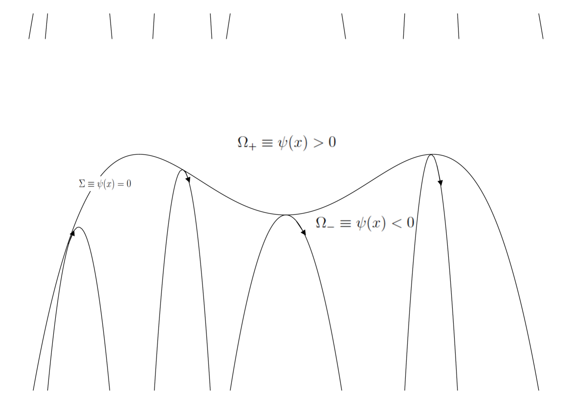
Figure 1. Pseudo-convexity: the characteristic curves which are tangent to $\Sigma$ stay in the “past”, below $\Sigma$.

Counterexamples

Theorem 8.9.2 in [6] displays a construction due to P. Cohen: there exists a smooth non-vanishing complex vector field in two dimensions,

$$\mathcal{C}=\partial_{t}+ib(t,x)\partial_{x},\quad b\in C^{{\infty}}(\mathbb{R}^{2}),$$

and a $C^{{\infty}}$ function $u$ in $\mathbb{R}^{2}$ with support equal to $\{t\geq 0\}$ such that $\mathcal{C}u=0$. Although the construction of that counterexample is an outstanding achievement, it turns out that the vector field $\mathcal{C}$ does not satisfy the Nirenberg-Treves condition $(P)$ (see e.g. Chapter 26 in [7]) and thus is not locally solvable. Note that this operator has simple characteristics as a first-order operator but has complex-valued coefficients (see also the study of complex vector fields by F. Treves & M. Strauss [18] and the X. Saint Raymond’s article [16]). There is a version of Hörmander’s theorem for operators with complex coefficients, but it requires a specific additional condition, the so-called principal normality (see (28.2.8) in [7]), which does not hold for $\mathcal{C}$.

On the other hand, S. Alinhac and S. Baouendi constructed in [2] the following counterexample: Let us consider the wave operator in 2-space dimension,

$$\partial_{t}^{2}-\partial_{x}^{2}-\partial_{y}^{2}=\square.$$

There exists $V,u\in C^{{\infty}}(\mathbb{R}^{3})$ with

(1.9) $$\operatorname{supp}u=\{y\geq 0\},\quad\square u+Vu=0.$$

Note that this operator is with constant coefficients, so that the characteristics are straight lines and the tangential ones are included in the boundary $y=0$, violating the pseudo-convexity hypothesis. This problem is easily proven to be ill-posed since it is non hyperbolic with respect to the time-like hypersurface $y=0$. The construction of this counterexample is a highly non-trivial task and this result appears as the most significant counterexample to Cauchy uniqueness. We note in particular that this constant coefficient operator (also of real principal type) is locally solvable, which is not the case of $\mathcal{C}$. As a result, the non-uniqueness property (1.9) is somehow more interesting for an operator having plenty of local solutions. The article [1] contains much more information on non-uniqueness results.

A recurrent question about the counterexample (1.9) was for long time if such a phenomenon could hold if $V$ does not depend on the time variable. A negative answer was given by D. Tataru’s [19], L. Hörmander’s [8], L. Robbiano & C. Zuily in [15] who proved uniqueness for $\square+V(t,x,y)$ with respect to $\{y=0\}$ when $V$ is a smooth function depending analytically of the variable $t$. Several geometric statements are given in that series of articles which go much beyond this example.

Another outstanding and still open question is linked to the Alinhac-Baouendi counterexample: is it possible to construct a counterexample (1.9) when $V$ is smooth and real-valued? The construction of [2] is using a complex-valued potential $V$ and one may conjecture that (1.9) with $V$ real-valued is impossible, but a proof of this uniqueness conjecture would certainly require other tools than Carleman’s standard estimates.

1.2. The Ionescu-Klainerman model problem

Their statement

We consider the wave operator in $\mathbb{R}_{t}\times\mathbb{R}^{d}_{x}$ defined by

(1.10) $$\square=\partial_{t}^{2}-\sum_{1\leq j\leq d}\partial_{x_{j}}^{2},$$

and let $\Omega$ be the open set defined by

(1.11) $$\Omega=\{(t,x)\in\mathbb{R}\times\mathbb{R}^{d},\quad|x|>1+|t|\}.$$

Theorem 1.1 (Theorem 1.1 in [11]).

Let $u\in C^{2}(\overline{\Omega})$ vanishing on $\partial\Omega$ such that the following pointwise inequality holds in $\Omega$,

(1.12) $$|\square u|\leq C\bigl{(}|u|+|\partial_{t}u|+|\nabla_{x}u|\bigr{)},$$

for some fixed constant $C$. Then $u$ vanishes on $\Omega$.

This result contains several interesting features: in the first place, the function $u$ is defined only on $\overline{\Omega}$ and the equation holds in $\Omega$, whose boundary is characteristic for $\square$. Also $u$ is only assumed to vanish on $\partial\Omega$ and no vanishing of any first derivative is required although the operator is second-order.

Comments

Since we intend to provide a more general statement with an invariant hypothesis, we start with a few comments on the above result. First of all, we note that the boundary $\partial\Omega$ is the union of two transversal characteristic hypersurfaces $\Sigma_{+},\Sigma_{-}$ with

$$\Sigma_{+}=\{(t,x),|x|=1+t,t\geq 0\},\quad\Sigma_{-}=\{(t,x),|x|=1-t,t\leq 0\},$$

and $\Omega=\{(t,x),|x|>1+t\text{ and }|x|>1-t\}.$ Moreover, since the function $u$ belongs to $C^{2}(\overline{\Omega})$, there exists $\widetilde{u}\in C^{2}(\mathbb{R}^{1+d})$ such that $\widetilde{u}_{|\overline{\Omega}}=u$. We can now take advantage of the fact that the boundary of $\Omega$ is the union of two characteristic hypersurfaces on which $u$ vanishes to prove that

$$v=\widetilde{u}\mathbf{1}_{\overline{\Omega}}$$

does satisfy the differential inequality (1.12) (and is supported in $\overline{\Omega}$). It is then enough to find a pseudo-convex hypersurface with equation $\{\psi=0\}$ whose epigraph $\{\psi\geq 0\}$ contains $\overline{\Omega}$ to apply (a slight modification) of Hörmander’s uniqueness theorem under a pseudo-convexity assumption to obtain the result. In particular, there is no need for a cutoff function supported inside $\Omega$ as in [11]. The details of our arguments are given below, but we hope that these short indications could convince the reader that a geometric statement is at hand.

The characteristic Cauchy problem

In Section 1.1, we gave results concerning the non-characteristic Cauchy problem for second-order operators with real coefficients. The main reason for these restrictions is that the pseudo-convexity hypothesis (1.8) has a very simple geometric formulation in that framework. However, uniqueness results and pseudo-convexity hypotheses can be expressed even for a characteristic hypersurface (and higher order operators). We may nevertheless say that, generically, characteristic problems do not have uniqueness (see e.g. Theorem 5.2.1 in [6]) and that the pseudo-convexity assumption (see (5.3.11) in [6]) does not hold in the model case above neither for $\Sigma_{+}$ nor for $\Sigma_{-}$.

An interesting phenomenon unraveled by Theorem 1.1 is that, although there is no uniqueness across any of the characteristic hypersurfaces $\Sigma_{\pm}$, the fact that the solution of the differential inequality is vanishing on the boundary of $\Omega$ and that $\Sigma_{+},\Sigma_{-}$ are intersecting transversally is indeed producing a uniqueness result.

1.3. Statement of our result

We consider a second-order differential operator $P$ in an open set $\mathcal{U}$ of $\mathbb{R}^{n}$ ($n\geq 3$) with real principal symbol

(1.13) $$p(x,\xi)=\langle Q(x)\xi,\xi\rangle,$$

where $Q(x)$ is a real symmetric matrix, a $C^{1}$ function of $x$, with signature $(n-1,1)$, i.e. with $(n-1)$ positive eigenvalues, 1 negative eigenvalue.

Note that it is in particular the case of the Wave operator in a Lorentzian manifold (the standard wave equation in $\mathbb{R}^{1+d}$ is $c^{-2}\partial_{t}^{2}-\Delta_{y}$ whose symbol is $-c^{-2}\tau^{2}+|\eta|^{2}$, indeed a quadratic form with signature $(n-1,1)$). We assume also that the coefficients of the lower order terms in $P$ are bounded measurable.

$\bullet$ Let $\phi_{+},\phi_{-}:\mathcal{U}:\rightarrow\mathbb{R}$ be two $C^{2}$ functions such that

(1.14) $$d\phi_{+}\not=0\text{ at }\phi_{+}=0,\qquad d\phi_{-}\not=0\text{ at }\phi_{-}=0,$$

(1.15) $$d\phi_{+}\wedge d\phi_{-}\not=0\text{ at $\phi_{+}=\phi_{-}=0$}.$$

$\bullet$ We define the open set

(1.16) $$\Omega=\{x\in\mathcal{U},\ \phi_{+}(x)>0\text{ and }\phi_{-}(x)>0\},$$

and we have from the above assumptions

$$\partial\Omega=\{x\in\mathcal{U},\ \phi_{+}(x)=0\text{ and }\phi_{-}(x)\geq 0\}\\ \cup\{x\in\mathcal{U},\ \phi_{-}(x)=0\text{ and }\phi_{+}(x)\geq 0\}.$$

$\bullet$ We shall also assume that the hypersurfaces $\Sigma_{+},\Sigma_{-}$ defined by

(1.17) $$\Sigma_{\pm}=\{x\in\mathcal{U},\phi_{\pm}(x)=0\},$$

are both characteristic, i.e.

(1.18) $$\forall x\in\Sigma_{+},\langle Q(x)d\phi_{+}(x),d\phi_{+}(x)\rangle=0,\quad\forall x\in\Sigma_{-},\langle Q(x)d\phi_{-}(x),d\phi_{-}(x)\rangle=0.$$

$\bullet$ Moreover, we shall assume that

(1.19) $$\forall x\in\Sigma_{+}\cap\Sigma_{-},\quad\langle Q(x)d\phi_{+}(x),d\phi_{-}(x)\rangle>0.$$

Note that these assumptions hold in the model case of  Section 1.2: with

$$\phi_{\pm}=|y|-1\mp t,\quad\mathcal{U}=\{(t,y)\in\mathbb{R}\times(\mathbb{R}^{d}\backslash\{0\})\},$$

we have indeed for $y\not=0$ (which holds at $\Sigma_{+}\cap\Sigma_{-}$ since there $t=0,|y|=1$),

$$d\phi_{+}\wedge d\phi_{-}=\bigl{(}\frac{y}{|y|}\cdot dy-dt\bigr{)}\wedge\bigl{(}\frac{y}{|y|}\cdot dy+dt\bigr{)}=2\frac{y}{|y|}\cdot dy\wedge dt\not=0,$$

and for this model-case we have

$$\langle Q(x)d\phi_{+}(x),d\phi_{-}(x)\rangle=-\frac{\partial\phi_{+}}{\partial t}\frac{\partial\phi_{-}}{\partial t}+\frac{\partial\phi_{+}}{\partial y}\cdot\frac{\partial\phi_{-}}{\partial y}=1+\frac{y}{|y|}\cdot\frac{y}{|y|}=2.$$

We are ready to state our unique continuation result.

Theorem 1.2.

Let $\mathcal{U},P,Q,\Omega,\Sigma_{\pm},$ as above in (1.13)—(1.19). Let $u$ be a function in $C^{2}(\overline{\Omega})$ such that,

(1.20) $$\exists C\geq 0,\forall x\in\Omega,\quad|(Pu)(x)|\leq C\bigl{(}|(\nabla_{x}u)(x)|+|u(x)|\bigr{)},$$

(1.21) $$u_{|\partial\Omega}=0.$$

Then $u$ vanishes in a neighborhood of $\Sigma_{+}\cap\Sigma_{-}$.

2. Proof of a differential inequality

2.1. Extending the solution

Our function $u$ in Theorem 1.2 belongs to $C^{2}(\overline{\Omega})$ and thus there exists a function $\widetilde{u}\in C^{2}(\mathcal{U})$ such that

$$\widetilde{u}_{|\overline{\Omega}}=u,\quad\widetilde{u}=0\text{ at $\partial\Omega$.}$$

We may thus define a function $v$ as a function in $L^{{\infty}}_{loc}(\mathcal{U})$ by

(2.1) $$v(x)=\mathbf{1}_{\overline{\Omega}}(x)\widetilde{u}(x),$$

and we have of course that

(2.2) $$\operatorname{supp}v\subset\overline{\Omega},\quad v_{|\overline{\Omega}}=u.$$

We claim now that $v$, which is defined “globally” in $\mathcal{U}$, does satisfy some differential inequality, at least in a neighborhood of $\Sigma_{+}\cap\Sigma_{-}$. The sequel of this subsection is actually devoted to the proof of such a differential inequality. Taking

$$(\underbrace{\phi_{+}}_{y_{1}},\underbrace{\phi_{-}}_{y_{2}},\underbrace{y_{3}}_{\in\mathbb{R}^{n-2}}),$$

as $C^{2}$ coordinates near a point $x_{0}$ of $\Sigma_{+}\cap\Sigma_{-}$, we may consider there $\widetilde{u}$ as a $C^{2}$ function $\tilde{u}_{\kappa}(y_{1},y_{2},y_{3})$ defined by

$$\tilde{u}_{\kappa}(y)=\widetilde{u}(\kappa(y)),$$

where $\kappa$ is a local $C^{2}$ diffeomorphism from $(-1,1)^{n}$ onto a neighborhood $\mathcal{U}_{0}$ of $x_{0}$,

$$\tilde{u}_{\kappa}(0,y_{2},y_{3})=0\text{ \quad for $y_{2}\geq 0,$}$$

$$\tilde{u}_{\kappa}(y_{1},0,y_{3})=0\text{ \quad for $y_{1}\geq 0$}.$$

We find that the principal symbol of the operator $P$ may be then written as

$$p_{\kappa}(y,\eta)=p\bigl{(}\kappa(y),{{}^{t}}\!\kappa^{\prime}(y)^{-1}\eta\bigr{)}=\langle Q(\kappa(y)){{}^{t}}\!\kappa^{\prime}(y)^{-1}\eta,{{}^{t}}\!\kappa^{\prime}(y)^{-1}\eta\rangle,$$

so that defining the symmetric $n\times n$ matrix

$$Q_{\kappa}(y)=\kappa^{\prime}(y)^{-1}Q(\kappa(y)){{}^{t}}\!\kappa^{\prime}(y)^{-1}=\bigl{(}b_{jk}(y)\bigr{)}_{1\leq j,k\leq n},$$

the fact that $\Sigma_{\pm}$ are characteristic may be expressed by

$$b_{11}(y)=b_{22}(y)=0,\quad\max_{1\leq j\leq n}|y_{j}|<1.$$

Note that since $Q$ is assumed to be $C^{1}$ and $\kappa$ is $C^{2}$ we still have the $C^{1}$ regularity for $Q_{\kappa}$. As a result, the principal part $p_{\kappa}(y,D_{y})$ can be written (near 0) as

(2.3) $$-p_{\kappa}(y,D_{y})=2b_{1,2}(y)\frac{\partial^{2}}{\partial y_{1}\partial y_{2}}+\sum_{j\geq 3}2b_{1,j}(y)\frac{\partial^{2}}{\partial y_{1}\partial y_{j}}+\sum_{j\geq 3}2b_{2,j}(y)\frac{\partial^{2}}{\partial y_{2}\partial y_{j}}\\ +\sum_{3\leq j,k\leq n}b_{j,k}(y)\frac{\partial^{2}}{\partial y_{j}\partial y_{k}}.$$

Also we note that, with $\nu=\kappa^{-1}$ and $w\in C^{1}(\mathcal{U}_{0})$, we have with $x=\kappa(y),y=\nu(x)$,

(2.4) $$\frac{\partial w}{\partial x_{j}}=\sum_{1\leq k\leq n}\underbrace{\frac{\partial y_{k}}{\partial x_{j}}}_{\in C^{1}(\mathcal{U}_{0})}\frac{\partial w_{\kappa}}{\partial y_{k}},\qquad w_{\kappa}=w\circ\kappa.$$

Let us now define with $H$ standing for indicator function of $\mathbb{R}_{+}$ (Heaviside function),

$$v_{\kappa}(y)=H(y_{1})H(y_{2})\tilde{u}_{\kappa}(y_{1},y_{2},y_{3}).$$

Lemma 2.1.

Let $U$ be a $C^{2}$ real-valued function defined for

$$(y_{1},y_{2},y_{3})\in(-1,1)\times(-1,1)\times(-1,1)^{n-2},$$

and such that

(2.5) $$U(0,y_{2},y_{3})=0\text{ \quad for $y_{2}\geq 0,$}$$

(2.6) $$U(y_{1},0,y_{3})=0\text{ \quad for $y_{1}\geq 0$}.$$

Then defining $V(y)=H(y_{1})H(y_{2})U(y_{1},y_{2},y_{3}),$ we have

(2.7) $$\frac{\partial V}{\partial y_{1}}=H(y_{1})H(y_{2})\frac{\partial U}{\partial y_{1}},\quad\frac{\partial V}{\partial y_{2}}=H(y_{1})H(y_{2})\frac{\partial U}{\partial y_{2}},$$

(2.8) $$\frac{\partial^{2}V}{\partial y_{1}\partial y_{2}}=H(y_{1})H(y_{2})\frac{\partial^{2}U}{\partial y_{1}\partial y_{2}},$$

(2.9) $$\text{for $j\geq 3$, \ }\frac{\partial^{2}V}{\partial y_{1}\partial y_{j}}=H(y_{1})H(y_{2})\frac{\partial^{2}U}{\partial y_{1}\partial y_{j}},\quad\frac{\partial^{2}V}{\partial y_{2}\partial y_{j}}=H(y_{1})H(y_{2})\frac{\partial^{2}U}{\partial y_{2}\partial y_{j}},$$

(2.10) $$\text{for $j,k\geq 3$, \ }\frac{\partial^{2}V}{\partial y_{j}\partial y_{k}}=H(y_{1})H(y_{2})\frac{\partial^{2}U}{\partial y_{j}\partial y_{k}}.$$

Proof.

We start with (2.7): we note first that both sides of the equalities are making sense, left-hand sides as distribution derivatives of the $L^{{\infty}}_{loc}$ function $V$ and right-hand sides as products of $C^{1}$ functions $\partial U/\partial y_{j}$ by the $L^{{\infty}}_{loc}$ function $H(y_{1})H(y_{2})$. We need only to use Leibniz formula using Assumptions (2.5), (2.6), so that

$$\frac{\partial V}{\partial y_{1}}=H(y_{1})H(y_{2})\frac{\partial U}{\partial y_{1}}+\underbrace{\bigl{(}\delta_{0}(y_{1})\otimes H(y_{2})\bigr{)}}_{\text{measure}}\underbrace{U}_{\begin{subarray}{c}\text{continuous}\\ \text{function}\end{subarray}}.$$

Let $\varphi\in C^{{\infty}}_{\textit{c}}\bigl{(}(-1,1)^{n}=J\bigr{)}$. We have with brackets of duality $\langle\mathscr{D}^{\prime(0)}(J),C^{0}_{c}(J)\rangle$ (here $\mathscr{D}^{\prime(0)}(J)$ stands for the Radon measures on $J$),

$$\langle\bigl{(}\delta_{0}(y_{1})\otimes H(y_{2})\bigr{)}U,\varphi\rangle=\langle\bigl{(}\delta_{0}(y_{1})\otimes H(y_{2})\bigr{)},U\varphi\rangle\\ =\iint H(y_{2})U(0,y_{2},y_{3})\varphi(0,y_{2},y_{3})dy_{2}dy_{3}=0,$$

thanks to (2.5); similarly, we obtain the second formula in (2.7), using (2.6). Starting from the now proven (2.7), Formula (2.9) is trivial and (2.10) is an immediate consequence of the definition of $V$. We are left with (2.8): we have from (2.7), noting that $\partial U/\partial y_{2}$ is a $C^{1}$ function,

(2.11) $$\frac{\partial}{\partial y_{1}}\left\{\frac{\partial V}{\partial y_{2}}\right\}=\frac{\partial}{\partial y_{1}}\left\{H(y_{1})H(y_{2})\frac{\partial U}{\partial y_{2}}\right\}=\bigl{(}\delta_{0}(y_{1})\otimes H(y_{2})\bigr{)}\frac{\partial U}{\partial y_{2}}\\ +H(y_{1})H(y_{2})\frac{\partial^{2}U}{\partial y_{1}\partial y_{2}},$$

and with the above notations, for $\varphi\in C^{{\infty}}_{\textit{c}}(J)$, we have

(2.12) $$\langle\bigl{(}\delta_{0}(y_{1})\otimes H(y_{2})\bigr{)}\frac{\partial U}{\partial y_{2}},\varphi\rangle=\langle\bigl{(}\delta_{0}(y_{1})\otimes H(y_{2})\bigr{)},\frac{\partial U}{\partial y_{2}}\varphi\rangle\\ =\iint H(y_{2})\frac{\partial U}{\partial y_{2}}(0,y_{2},y_{3})\varphi(0,y_{2},y_{3})dy_{2}dy_{3}.$$

The identity (2.5) holds for $(y_{2},y_{3})\in(0,1)\times(-1,1)^{n-2}$, and thus the continuous function $\partial U/\partial y_{2}$ satisfies

$$\frac{\partial U}{\partial y_{2}}(0,y_{2},y_{3})=0\quad\text{for $(y_{2},y_{3})\in(0,1)\times(-1,1)^{n-2}$},$$

which implies from (2.12)

$$\bigl{(}\delta_{0}(y_{1})\otimes H(y_{2})\bigr{)}\frac{\partial U}{\partial y_{2}}=0,$$

so that (2.11) yields the sought (2.8). ∎

Lemma 2.2.

Let $U$ be a real-valued $C^{2}$ function defined on $(-1,1)^{n}$ satisfying the assumptions of Lemma 2.1. Let $B(y)=(\beta_{jk}(y))_{1\leq j\leq k}$ be a real symmetric matrix of class $C^{1}$ on $(-1,1)^{n}$ such that $\beta_{11}=\beta_{22}=0$. Then defining

(2.13) $$V(y)=H(y_{1})H(y_{2})U(y_{1},y_{2},y_{3}),$$

we have $\beta_{jk}\frac{\partial^{2}V}{\partial y_{j}\partial y_{k}}\in L^{{\infty}}_{loc}$ for all $j,k\in\{1,\dots,n\}$ and

(2.14) $$\bigl{(}\langle B(y)\partial_{y},\partial_{y}\rangle V\bigr{)}(y)=H(y_{1})H(y_{2})\bigl{(}\langle B(y)\partial_{y},\partial_{y}\rangle U\bigr{)}(y),$$

(2.15) $$(\frac{\partial V}{\partial y})(y)=H(y_{1})H(y_{2})(\frac{\partial U}{\partial y})(y).$$

The proof of this lemma is an immediate consequence of Lemma 2.1.

∎

Lemma 2.3.

Let $U,V,B$ as in Lemma 2.2 such that there exists a constant $C\geq 0$ such that

(2.16) $$\forall y\in(-1,1)^{n}\text{ with $y_{1}>0$ and $y_{2}>0$},\quad|\bigl{(}\langle B(y)\partial_{y},\partial_{y}\rangle U\bigr{)}(y)|\\ \leq C\bigl{(}|(\nabla_{y}U)(y)|+|U(y)|\bigr{)}.$$

Then $\langle B(y)\partial_{y},\partial_{y}\rangle V,\nabla_{y}V,V$ are locally bounded measurable and

(2.17) $$\text{for almost all }y\in(-1,1)^{n},\quad|\bigl{(}\langle B(y)\partial_{y},\partial_{y}\rangle V\bigr{)}(y)|\\ \leq C\bigl{(}|(\nabla_{y}V)(y)|+|V(y)|\bigr{)}.$$

Proof.

Using (2.13), (2.14), (2.15) we obtain that $\langle B(y)\partial_{y},\partial_{y}\rangle V,\nabla_{y}V,V$ are locally bounded measurable and

$$|\bigl{(}\langle B(y)\partial_{y},\partial_{y}\rangle V\bigr{)}(y)| =H(y_{1})H(y_{2})|\bigl{(}\langle B(y)\partial_{y},\partial_{y}\rangle U\bigr{)}(y)|$$

$${\hskip 15.0pt}\leq H(y_{1})H(y_{2})C\bigl{(}|(\nabla_{y}U)(y)|+|U(y)|\bigr{)}$$

$${\hskip 15.0pt}{\hskip 15.0pt}=C\bigl{(}|(\nabla_{y}V)(y)|+|V(y)|\bigr{)}.$$

∎

Remark 2.4.

The reader may note that we have used (2.5),(2.6) (i.e. vanishing of $U$ on the boundary of $\{y_{1}>0,y_{2}>0\}$ and the fact that the boundary is characteristic, expressed in the $y$ coordinates by the equalities $\beta_{11}=\beta_{22}=0$. All these conditions are important to get Lemma 2.2. For instance, assuming only (2.5),(2.6), but $\beta_{11}\not=0$, we would have to calculate

$$\frac{\partial^{2}V}{\partial y_{1}^{2}} =\frac{\partial}{\partial y_{1}}\bigl{\{}\overbrace{(\delta_{0}(y_{1})\otimes H(y_{2}))U}^{=0\text{ from \eqref{0001}}}+H(y_{1})H(y_{2})\frac{\partial U}{\partial y_{1}}\bigr{\}}$$

$$=(\delta_{0}(y_{1})\otimes H(y_{2}))\frac{\partial U}{\partial y_{1}}+H(y_{1})H(y_{2})\frac{\partial^{2}U}{\partial y_{1}^{2}}$$

(2.18) $$=(\delta_{0}(y_{1})\otimes H(y_{2}))\frac{\partial U}{\partial y_{1}}(0,y_{2},y_{3})+H(y_{1})H(y_{2})\frac{\partial^{2}U}{\partial y_{1}^{2}},$$

and the term $\frac{\partial U}{\partial y_{1}}(0,y_{2},y_{3})$ can be non-zero (say for $U=y_{1}y_{2}$). The consequence of that situation would be that, even with $C=0$ in Assumption (2.16) and $\beta_{22}=0$, we would obtain the following equality for $V$

(2.19) $$\bigl{(}\langle B(y)\partial_{y},\partial_{y}\rangle V\bigr{)}(y)=(\delta_{0}(y_{1})\otimes H(y_{2}))\frac{\partial U}{\partial y_{1}}(0,y_{2},y_{3})\beta_{11}(0,y_{2},y_{3}),$$

where the rhs is a simple layer that cannot be controlled pointwise by $V$ or its first-order derivatives. The fact that $V$ inherits a differential inequality from $U$, assuming a simple vanishing of $U$ on the boundary $\partial\Omega$, is thus linked with the geometric situation: both hypersurfaces $\Sigma_{\pm}$ are characteristic for the operator $P$. Of course, we could have assumed a second-order vanishing (i.e. vanishing of the function and its first derivatives on $\partial\Omega$, an assumption which would allow us to get rid of the rhs in (2.19) since then, we would have ${\partial U}/{\partial y_{1}}(0,y_{2},y_{3})=0$), but we would have lost most of the flavour of the model case given in Section 1.2.

Remark 2.5.

Let $u$ be a function satisfying the assumptions of Theorem 1.2, let $v$ be defined by (2.1) and let $x_{0}$ be a given point in $\Sigma_{+}\cap\Sigma_{-}$. The assumptions (1.20), (1.21) and Lemma 2.3 imply that there exists a neighborhood $\mathcal{U}_{0}$ of $x_{0}$ and a constant $C_{0}\geq 0$ such that

(2.20) $$\forall x\in\mathcal{U}_{0},\quad|(Pv)(x)|\leq C_{0}\bigl{(}|(\nabla_{x}v)(x)|+|v(x)|\bigr{)},$$

(2.21) $$\operatorname{supp}v\subset\overline{\Omega},\quad v_{|\overline{\Omega}}=u.$$

As a result, to prove Theorem 1.2, we are reduced to proving that $v$ vanishes on a neighborhood of $x_{0}$ in $\mathcal{U}_{0}$.

Remark 2.6.

Building on Remark 2.4, we note that $u$ satisfies the differential inequality (1.20) only on $\Omega$, which is not a convenient situation to use Hörmander’s pseudo-convexity result. This is the main reason for which we have introduced the new function $v$ given by (2.1): we want to point out that the fact that $v$ is still satisfying some differential inequality (here (2.20)) is a consequence of three geometrical facts: first of all, $u$ is vanishing on $\partial\Omega$, next, both hypersurfaces $\Sigma_{\pm}$ are characteristic for $P$ and finally $\Sigma_{\pm}$ are transverse. The function $v$ is defined in a neighborhood of $\Sigma_{+}\cap\Sigma_{-}$, supported in $\overline{\Omega}$ and a satisfies a differential inequality: we are in good position to use the classical Carleman estimates, provided we find a suitable pseudo-convex hypersurface.

2.2. The sign condition

Lemma 2.7.

Let $\mathcal{U},Q,\phi_{\pm}$ as given in (1.13)—(1.19). We define

(2.22) $$\psi_{1}=\frac{1}{2}\bigl{(}\phi_{+}+\phi_{-}\bigr{)},\qquad\psi_{0}=\frac{1}{2}\bigl{(}\phi_{-}-\phi_{+}\bigr{)}.$$

Then we have ,

(2.23) $$\langle Q(x)d\psi_{1}(x),d\psi_{1}(x)\rangle>0>\langle Q(x)d\psi_{0}(x),d\psi_{0}(x)\rangle\quad\text{at }\Sigma_{+}\cap\Sigma_{-},$$

(2.24) $$\Omega=\{x\in\mathcal{U},\psi_{1}(x)>|\psi_{0}(x)|\},$$

(2.25) $$d\psi_{1}\wedge d\psi_{0}\not=0\quad\text{at }\Sigma_{+}\cap\Sigma_{-}.$$

Proof.

Properties (2.24)-(2.25) are obvious. Let us prove (2.23). From (1.18), we have

$$\langle Q(x)d\phi_{+}(x),d\phi_{+}(x)\rangle=0\ \text{at $\Sigma_{+}$},\quad\langle Q(x)d\phi_{-}(x),d\phi_{-}(x)\rangle=0\ \text{at $\Sigma_{-}$},$$

so that at $\Sigma_{+}\cap\Sigma_{-}$, since $\phi_{\pm}=\psi_{1}\mp\psi_{0}$,

$$\langle Q(x)d\psi_{1}(x),d\psi_{1}(x)\rangle\mp 2\langle Q(x)d\psi_{1}(x),d\psi_{0}(x)\rangle+\langle Q(x)d\psi_{0}(x),d\psi_{0}(x)\rangle=0,$$

implying

(2.26) $$\langle Q(x)d\psi_{1}(x),d\psi_{1}(x)\rangle+\langle Q(x)d\psi_{0}(x),d\psi_{0}(x)\rangle=0=\langle Q(x)d\psi_{1}(x),d\psi_{0}(x)\rangle.$$

As a consequence, we have from (1.19), at $\Sigma_{+}\cap\Sigma_{-}$,

$$0<\langle Q(x)d\phi_{+}(x),d\phi_{-}(x)\rangle=\langle Q(x)d\psi_{1}(x),d\psi_{1}(x)\rangle-\langle Q(x)d\psi_{0}(x),d\psi_{0}(x)\rangle,$$

and (2.26) yields

$$0<2\langle Q(x)d\psi_{1}(x),d\psi_{1}(x)\rangle\text{ and thus }\langle Q(x)d\psi_{0}(x),d\psi_{0}(x)\rangle<0,$$

which is the sought result. ∎

Remark 2.8.

Property (2.23) means that, near $\Sigma_{+}\cap\Sigma_{-}$, the hypersurface defined by $\{\psi_{0}=0\}$ is space-like whereas the hypersurface defined by $\{\psi_{1}=0\}$ is time-like.

2.3. Finding a pseudo-convex hypersurface

Let $p$ be given by (1.13) and let $\psi$ be a $C^{2}$ function defined on $\mathcal{U}$ such that $d\psi\not=0$ at $\psi=0$. We recall that the oriented hypersurface with equation $\{\psi=0\}$ is pseudo-convex with respect to $P$ whenever (1.8) holds.

Lemma 2.9.

Let $x_{0}\in\Sigma_{+}\cap\Sigma_{-}$ and let $\lambda>0$ be given. Then there exists a neighborhood $\mathcal{U}_{0,\lambda}$ of $x_{0}$ in $\mathcal{U}$ such that

$$\Omega\cap\mathcal{U}_{0,\lambda}\subset\{x\in\mathcal{U}_{0,\lambda},\psi_{1}(x)>\lambda\psi_{0}^{2}(x)\}.$$

Proof.

Assuming $\phi_{+}(x)>0,\phi_{-}(x)>0$, we find that

$$\psi_{1}(x)>|\psi_{0}(x)|\text{ and thus }\psi_{1}(x)>|\psi_{0}(x)|\geq\lambda\psi_{0}^{2}(x),$$

if $|\psi_{0}(x)|<1/\lambda$; since the latter condition defines a neighborhood of $x_{0}$, we obtain the result. ∎

Lemma 2.10.

Let $n\geq 2$ and let $M$ be an $n\times n$ real symmetric matrix with signature $(n-1,1)$. Let $\xi_{0},\xi$ be two non-zero vectors of $\mathbb{R}^{n}$ such that

$$\langle M\xi,\xi\rangle=0,\quad\langle M\xi_{0},\xi_{0}\rangle<0.$$

Then $\langle M\xi,\xi_{0}\rangle\not=0$.

Proof.

There exists a $n\times n$ invertible matrix $R$ such that

$${{}^{t}}\!RMR=\begin{pmatrix}I_{n-1}&0\\ 0&-1\end{pmatrix},$$

where $I_{n-1}$ is the identity matrix with size $n-1$. Defining

$$\eta_{0}=R^{-1}\xi_{0},\quad\eta=R^{-1}\xi,$$

we get two non-zero vectors $\eta_{0}=(\zeta_{0},\tau_{0})$, $\eta=(\zeta,\tau)$ of $\mathbb{R}^{n-1}\times\mathbb{R}$ such that, with standard dot-products in $\mathbb{R}^{n-1}$,

(2.27) $$|\zeta|^{2}=\tau^{2},\quad|\zeta_{0}|^{2}<\tau_{0}^{2}.$$

Note that since $(\zeta,\tau)\not=0$, the first equality implies that $\tau\not=0$. We have then $\langle M\xi,\xi_{0}\rangle=\zeta\cdot\zeta_{0}-\tau\tau_{0}$ and if we had $\zeta\cdot\zeta_{0}=\tau\tau_{0}$, this would give

$$|\tau\tau_{0}|=|\zeta\cdot\zeta_{0}|\leq|\zeta||\zeta_{0}|=|\tau||\zeta_{0}|\underbrace{<}_{\begin{subarray}{c}\tau\not=0\\ |\zeta_{0}|<|\tau_{0}|\end{subarray}}|\tau||\tau_{0}|,$$

which is impossible. As a result, we get indeed $\langle M\xi,\xi_{0}\rangle\not=0$. ∎

Proposition 2.11.

Let $x_{0}\in\Sigma_{+}\cap\Sigma_{-}$, and let $\psi_{0},\psi_{1}$ be defined in Lemma 2.7. There exists $\lambda>0$ such that

$$\forall\xi\in\mathbb{S}^{n-1},\quad p(x_{0},\xi)=H_{p}{(\psi_{1}-\lambda\psi_{0}^{2})}(x_{0},\xi)=0\Longrightarrow H_{p}^{2}(\psi_{1}-\lambda\psi_{0}^{2})(x_{0},\xi)<0.$$

This means that the oriented hypersurface $S$ with equation $\{\psi_{1}-\lambda\psi_{0}^{2}=0\}$ is pseudo-convex with respect to the operator $P$ at $x_{0}$ (note that the first inequality in (2.23) ensures that $S$ is non-characteristic for $P$).

Proof.

We have

$$p(x,\xi)=\langle Q(x)\xi,\xi\rangle,\quad\frac{1}{2}H_{p}(\psi)(x,\xi)=\langle Q(x)\xi,d\psi(x)\rangle,$$

(2.28) $$\frac{1}{2}H_{p}^{2}(\psi)(x,\xi)=\sum_{1\leq j\leq n}\frac{\partial p}{\partial\xi_{j}}\Bigl{(}\langle\frac{\partial Q}{\partial x_{j}}\xi,d\psi(x)\rangle+\langle Q(x)\xi,d\frac{\partial\psi}{\partial x_{j}}\rangle\Bigr{)}\\ -\hskip-25.0pt\underbrace{\langle\frac{\partial Q}{\partial x}\xi,\xi\rangle}_{\begin{subarray}{c}\text{covector with }\\ \text{components $\langle\partial_{x_{j}}Q(x)\xi,\xi\rangle$ }\end{subarray}}\hskip-20.0pt\cdot\underbrace{Q(x)d\psi(x)}_{\begin{subarray}{c}\text{vector}\end{subarray}}.$$

We note that $H_{p}^{2}(\psi)$ is a quadratic form in the variable $\xi$, with coefficients depending polynomially on $Q(x),\nabla_{x}Q(x),\nabla_{x}\psi,\nabla_{x}^{2}\psi$.

Let $\xi\in\mathbb{S}^{n-1}$ such that at $x_{0}\in\Sigma_{+}\cap\Sigma_{-}$, $p(x_{0},\xi)=H_{p}{(\psi_{1}-\lambda\psi_{0}^{2})}(x_{0},\xi)=0.$ Since $\psi_{0}(x_{0})=0$, we infer that

(2.29) $$\langle Q(x_{0})\xi,\xi\rangle=\langle Q(x_{0})\xi,d\psi_{1}(x_{0})\rangle=0,\quad\text{i.e.}\quad p(x_{0},\xi)=H_{p}{(\psi_{1})}(x_{0},\xi)=0.$$

We have also

$$H_{p}^{2}(\psi_{1}-\lambda\psi_{0}^{2})=H_{p}^{2}(\psi_{1})-\lambda H_{p}^{2}(\psi_{0}^{2})$$

and since $\psi_{0}(x_{0})=0$, we get

(2.30) $$H_{p}^{2}(\psi_{1}-\lambda\psi_{0}^{2})(x_{0},\xi)=H_{p}^{2}(\psi_{1})(x_{0},\xi)-2\lambda\bigl{(}H_{p}(\psi_{0})(x_{0},\xi)\bigr{)}^{2}.$$

Moreover, we have, using (2.29) and (2.23)

$$\langle Q(x_{0})\xi,\xi\rangle=\langle Q(x_{0})\xi,d\psi_{1}(x_{0})\rangle=0,\quad\langle Q(x_{0})d\psi_{0}(x_{0}),d\psi_{0}(x_{0})\rangle<0.$$

We can use now Lemma 2.10 (with $\xi,\xi_{0}=d\psi(x_{0}),M=Q(x_{0})$) to obtain

$$\frac{1}{2}H_{p}(\psi_{0})(x_{0},\xi)=\langle Q(x_{0})\xi,d\psi_{0}(x_{0})\rangle\not=0.$$

We may thus define the positive number

(2.31) $$m_{0}=\min_{\begin{subarray}{c}\xi\in\mathbb{S}^{n-1}\text{such that }\\ \langle Q(x_{0})\xi,\xi\rangle=\langle Q(x_{0})\xi,d\psi_{1}(x_{0})\rangle=0\end{subarray}}\overbrace{2|\langle Q(x_{0})\xi,d\psi_{0}(x_{0})\rangle|}^{=|H_{p}(\psi_{0})(x_{0},\xi)|}.$$

Since we have

$$p(x_{0},\xi)=\langle Q(x_{0})\xi,\xi\rangle,\quad H_{p}(\psi_{0})=2\langle Q(x_{0})\xi,d\psi_{0}(x)\rangle,$$

assuming with $m_{0}$ defined in (2.31), that

(2.32) $$\lambda>\frac{\max_{\xi\in\mathbb{S}^{n-1}}H_{p}^{2}(\psi_{1})(x_{0},\xi)}{2m_{0}^{2}}=\lambda_{0},$$

we obtain from (2.30) that, if for $\xi\in\mathbb{S}^{n-1}$, we have $p(x_{0},\xi)=H_{p}(\psi_{1}-\lambda\psi_{0}^{2})(x_{0},\xi)=0,$ then we get

$$H_{p}^{2}(\psi_{1}-\lambda\psi_{0}^{2})(x_{0},\xi)<0,$$

since (2.32) implies for any $\xi\in\mathbb{S}^{n-1}$ such that $p(x_{0},\xi)=H_{p}(\psi_{1}-\lambda\psi_{0}^{2})(x_{0},\xi)=0$, that $H_{p}(\psi_{0})(x_{0},\xi)\not=0$ and

$$\lambda>\frac{H_{p}^{2}(\psi_{1})(x_{0},\xi)}{2\bigl{(}H_{p}(\psi_{0})(x_{0},\xi)\bigr{)}^{2}}\text{ and thus }H_{p}^{2}(\psi_{1})(x_{0},\xi)-2\lambda\bigl{(}H_{p}(\psi_{0})(x_{0},\xi)\bigr{)}^{2}<0,$$

yielding the sought result. ∎

3. Proof of Theorem 1.2

3.1. A slightly different question

Going back to the unique continuation question that we have to solve here, we may start looking again at our Remarks 2.4, 2.5. We have indeed a differential inequality on some open set $\mathcal{U}_{0}$

(3.1) $$|(Pv)(x)|\leq C_{0}\bigl{(}|(\nabla_{x}v)(x)|+|v(x)|\bigr{)},$$

where $P$ is a second-order differential operator with $C^{1}$ coefficients and also, defining

$$\psi=\psi_{1}-\lambda\psi_{0}^{2},$$

we know from Proposition 2.11 that the hypersurface $\{\psi=0\}$ is pseudo-convex with respect to $P$. Moreover we know that the function $v$ is vanishing on the open set $\{x\in\mathcal{U}_{0},\psi(x)<0\}$ (cf. Lemma 2.9) (maybe with a smaller neighborhood of $x_{0}$ than $\mathcal{U}_{0}$).

It seems straightforward to apply now Theorem 8.9.1 in [6] to obtain that $v$ should vanish near $\{\psi=0\}$ and give a positive answer to the question raised in Remark 2.5. However, we have to pay attention to the regularity at our disposal for the function $v$: we know that $v,\nabla v$ are bounded measurable functions, so in particular $v$ belongs to the Sobolev space $H^{1}_{loc}(\mathcal{U}_{0})$. Nevertheless our Remark 2.4 and the calculation (2.18) show that the simple vanishing of $u$ at $\partial\Omega$ leaves open the possibility of having for $\nabla^{2}v$ a simple layer so that we do not know if $v$ belongs to $H^{2}_{loc}(\mathcal{U}_{0})$, but only

(3.2) $$v\in H^{1}_{loc}(\mathcal{U}_{0}),\quad Pv\in L^{2}_{loc}(\mathcal{U}_{0}).$$

Although these assumptions should be sufficient for the classical theorem to hold, we have some checking to perform on this matter and we need to show that the classical assumption $v\in H^{2}_{loc}(\mathcal{U}_{0})$ can be weakened down to (3.2).

3.2. Invariance

Let us start with checking some easy facts. In the first place, let

$$P=\langle Q(x)\partial_{x},\partial_{x}\rangle+b(x)\cdot\partial_{x}+c(x)$$

be a differential operator with $C^{1}$ real coefficients in the principal part ($Q$ is a $C^{1}$ symmetric matrix) and $b,c$ are bounded measurable. Then the differential inequality is invariant by a $C^{2}$ change of coordinates. Let

$$\kappa:\mathcal{V}_{0}\rightarrow\mathcal{U}_{0}\quad\text{be a $C^{2}$ diffeomorphism}.$$

With standard notations we have

(3.3) $$\frac{\partial}{\partial x_{j}}=\sum_{k}\frac{\partial y_{k}}{\partial x_{j}}\frac{\partial}{\partial y_{k}},\quad\partial_{x}={{}^{t}}\!\kappa^{\prime}(y)^{-1}\partial_{y},$$

(3.4) $$\kappa^{*}(P)=\langle\kappa^{\prime}(y)Q(\kappa(y)){{}^{t}}\!\kappa^{\prime}(y)^{-1}\partial_{y},\partial_{y}\rangle+b(\kappa(y))\cdot{{}^{t}}\!\kappa^{\prime}(y)^{-1}\partial_{y}+c(\kappa(y)),$$

and since $\kappa^{\prime}(y)$ is $C^{1}$, the new matrix $\kappa^{\prime}(y)Q(\kappa(y)){{}^{t}}\!\kappa^{\prime}(y)^{-1}$ is still $C^{1}$ and the lower order terms are bounded measurable, whereas the differential inequality (3.1) becomes with $\kappa^{*}(v)=v\circ\kappa$, denoted by $v_{\kappa}$

$$|\bigl{(}\kappa^{*}(P)v_{\kappa}\bigr{)}(y)|\leq C_{0}\bigl{(}|({{}^{t}}\!\kappa^{\prime}(y)^{-1}(\nabla_{y}v_{\kappa})(y)|+|v_{\kappa}(y)|\bigr{)},$$

implying in the $y$-coordinates an inequality of the same type as (3.1). Assuming that the hypersurface with equation $\{\psi=0\}$ is non-characteristic is also invariant as well as the regularity of $\psi\circ\kappa$ if $\psi$ and $\kappa$ are assumed to be $C^{2}$.

Also the pseudo-convexity Assumption (1.8) is invariant by change of $C^{2}$ coordinates: let us assume that it holds in the $x$-coordinates with

$$p(x,\xi)=\langle Q(x)\xi,\xi\rangle,\quad\text{$Q$ real symmetric $C^{1}$ matrix, $\psi\in C^{2}$ such that \eqref{hormander} holds.}$$

We have now

$$p_{\kappa}(y,\eta)=\langle\kappa^{\prime}(y)^{-1}Q(\kappa(y)){{}^{t}}\!\kappa^{\prime}(y)^{-1}\eta,\eta\rangle=p\bigl{(}\kappa(y),{{}^{t}}\!\kappa^{\prime-1}(y)\eta\bigr{)},\quad\psi_{\kappa}=\psi\circ\kappa.$$

Let us assume that

$$p_{\kappa}(y_{0},\eta)=H_{p_{\kappa}}(\psi_{\kappa})(y_{0},\eta)=0,\eta\not=0.$$

Assuming that $Q,\kappa$ are smooth functions, we find immediately

$$H_{p_{\kappa}}^{2}(\psi_{\kappa})=\left\{p_{\kappa},\left\{p_{\kappa},\psi_{\kappa}\right\}\right\}=\bigl{(}H_{p}^{2}(\psi)\bigr{)}\circ\kappa.$$

We may regularize $Q$ and $\kappa$ to get the same result for $Q$ of class $C^{1}$, $\kappa$ a $C^{2}$ diffeomorphism, using the expression (2.28) which shows that $H_{p}^{2}(\psi)$ is a quadratic form in the variable $\xi$, with coefficients depending polynomially on $Q(x),\nabla_{x}Q(x),\nabla_{x}\psi,\nabla_{x}^{2}\psi$.

3.3. Mollifiers

Thanks to Theorems 8.6.3 and 8.3.1 in [6], the pseudo-convexity hypothesis on $\psi$ expressed by Proposition 2.11 allows us to find a smooth real-valued function $\phi$ defined on a neighborhood $\mathcal{U}_{0}$ of $x_{0}$ and constants $C_{0},\lambda_{1}$ such that

$$d\phi\not=0,\quad\{x\in\mathcal{U}_{0},\phi(x)<0\}\subset\{x\in\mathcal{U}_{0},\psi(x)<0\},$$

$$\{x\in\mathcal{U}_{0},\phi(x)=0,\psi(x)\geq 0\}=\{x_{0}\},$$

so that all $w\in C^{{\infty}}_{\textit{c}}(\mathcal{U}_{0})$, for all $\lambda\geq\lambda_{1}$,

(3.5) $$C_{0}\|e^{-\lambda\phi}Pw\|_{L^{2}}\geq\lambda^{1/2}\|e^{-\lambda\phi}\nabla w\|_{L^{2}}+\lambda^{3/2}\|e^{-\lambda\phi}w\|_{L^{2}}.$$

Let $v$ be a $H^{1}_{loc}$ function satisfying (2.20), which implies that $Pv$ belongs to $L^{2}_{loc}$, let $\chi\in C^{{\infty}}_{\textit{c}}(\mathcal{U}_{0})$. Let $\rho\in C^{{\infty}}_{\textit{c}}(\mathbb{R}^{n})$ supported in the unit ball, with integral 1 and let us set for $\epsilon>0$,

(3.6) $$\rho_{\epsilon}(z)=\epsilon^{-n}\rho(z/\epsilon).$$

Carleman Inequality (3.5) implies

$$C_{0}\|e^{-\lambda\phi}P(\rho_{\epsilon}\ast\chi v)\|_{L^{2}}\geq\lambda^{1/2}\|e^{-\lambda\phi}\nabla(\rho_{\epsilon}\ast\chi v)\|_{L^{2}}+\lambda^{3/2}\|e^{-\lambda\phi}(\rho_{\epsilon}\ast\chi v)\|_{L^{2}}.$$

Since $\phi$ is continuous and $\chi v$ belongs to $H^{1}_{c}(\mathcal{U}_{0})$ as well as $\chi v\ast\rho_{\epsilon}$ is supported in $\mathcal{U}_{0}$ for $\epsilon$ small enough, we find by standard mollifying arguments that the rhs has the limit

$$\lambda^{1/2}\|e^{-\lambda\phi}\nabla\chi v\|_{L^{2}}+\lambda^{3/2}\|e^{-\lambda\phi}\chi v\|_{L^{2}}.$$

Checking the lhs, we see that for $\chi_{0}\in C^{{\infty}}_{\textit{c}}(\mathcal{U}_{0})$, equal to 1 on a neighborhood of the support of $\chi$ (so that $\chi v\ast\rho_{\epsilon}$ is supported in $\{\chi_{0}=1\}$ for $\epsilon$ small enough) we find

$$P(\rho_{\epsilon}\ast\chi v)=\chi_{0}P\hat{\rho}(\epsilon D)\chi v=[\chi_{0}P,\hat{\rho}(\epsilon D)]\chi v+\hat{\rho}(\epsilon D)\chi_{0}Pv.$$

The term $\hat{\rho}(\epsilon D)\chi_{0}Pv$ goes to $\chi_{0}Pv$ in $L^{2}$ when $\epsilon$ goes to 0, since $Pv\in L^{2}_{loc}$. We need to prove that the first term goes to 0 in $L^{2}$. Proving this will mean that (3.5) holds for $w=\chi v$ and unique continuation will follow via standard arguments. For that purpose, let us state and prove the following lemma.

Lemma 3.1.

Let $a\in C^{1}_{c}(\mathbb{R}^{n})$, let $v\in H^{1}_{c}(\mathbb{R}^{n})$. Then, with $\rho$ as above, we have

$$\lim_{\epsilon\rightarrow 0_{+}}\Bigl{(}a\partial_{x}^{2}(\rho_{\epsilon}\ast v)-\rho_{\epsilon}\ast\bigl{(}a\partial_{x}^{2}v\bigr{)}\Bigr{)}=0,\quad\text{in $L^{2}(\mathbb{R}^{n})$},$$

where $\partial_{x}^{2}b$ stands for the Hessian matrix of $b$.

N.B. The function $\partial_{x}^{2}(\rho_{\epsilon}\ast v)$ is smooth compactly supported (thus in $L^{2}$) and bounded in $H^{-1}$ when $\epsilon$ goes to 0. As a result the product $a\partial_{x}^{2}(\rho_{\epsilon}\ast v)$ is $C^{1}_{c}$ and bounded in $H^{-1}$. On the other hand $a\partial_{x}^{2}v$ belongs to $H^{-1}_{c}$ and thus $\rho_{\epsilon}\ast(a\partial_{x}^{2}v)$ is smooth compactly supported and bounded in $H^{-1}$.

Proof.

We have with obvious notations, for $v\in H^{1}_{c}$,

$$D_{\epsilon}(v) =\bigl{(}a\partial_{x}^{2}(\rho_{\epsilon}\ast v)\bigr{)}(x)-\bigl{(}\rho_{\epsilon}\ast\bigl{(}a\partial_{x}^{2}v\bigr{)}\bigr{)}(x)$$

$$=a(x)\int(\nabla\rho_{\epsilon})(x-y)(\nabla v)(y)dy-\overbrace{\int\underbrace{\rho_{\epsilon}(x-y)a(y)}_{\in H^{1}(y)}\underbrace{\nabla^{2}v(y)}_{\in H^{-1}(y)}dy}^{\text{a bracket of duality}}$$

$$=\int a(x)(\nabla\rho_{\epsilon})(x-y)(\nabla v)(y)dy-\int(\nabla\rho_{\epsilon})(x-y)a(y)\nabla v(y)dy$$

$$\hskip 195.0pt+\int\rho_{\epsilon}(x-y)\nabla a(y)\nabla v(y)dy.$$

The very last term has limit (the matrix) $\nabla a\nabla v$ in $L^{2}(\mathbb{R}^{n})$. Defining the first two terms as $\tilde{D}_{\epsilon}(v)$, we get

$$\tilde{D}_{\epsilon}(v) =\int\bigl{(}a(x)-a(y)\bigr{)}(\nabla\rho_{\epsilon})(x-y)\nabla v(y)dy$$

$$=\int_{0}^{1}\int\nabla a(y+\theta(x-y))\cdot(x-y)(\nabla\rho_{\epsilon})(x-y)\nabla v(y)dyd\theta$$

$$=\int_{0}^{1}\int\nabla a(y+\theta(x-y))\cdot\frac{(x-y)}{\epsilon}(\nabla\rho)_{\epsilon}(x-y)\nabla v(y)dyd\theta$$

$$=\int_{0}^{1}\int\nabla a(x-\epsilon(1-\theta)z)\cdot z(\nabla\rho)(z)\nabla v(x-\epsilon z)dzd\theta.$$

The function $z_{k}{\partial\rho}/{\partial z_{j}}$ is smooth compactly supported with integral $-\delta_{j,k}$ and thus

$$\lim_{\epsilon\rightarrow 0_{+}} \int_{0}^{1}\int\partial_{k}a(x-\epsilon(1-\theta)z)\cdot z_{k}(\partial_{j}\rho)(z)\partial_{l}v(x-\epsilon z)dzd\theta$$

$$=\lim_{\epsilon\rightarrow 0_{+}}\Bigl{\{}\int_{0}^{1}\int\bigl{(}\partial_{k}a(x-\epsilon(1-\theta)z)-\partial_{k}a(x)\bigr{)}\cdot z_{k}(\partial_{j}\rho)(z)\partial_{l}v(x-\epsilon z)dzd\theta$$

$$\hskip 200.0pt+(\partial_{k}a)(x)\int z_{k}(\partial_{j}\rho)(z)\partial_{l}v(x-\epsilon z)dz\Bigr{\}}$$

$$=-(\partial_{j}a)(x)(\partial_{l}v)(x),\quad\text{in $L^{2}(\mathbb{R}^{n})$,}$$

since

$$|\partial_{k}a(x-\epsilon(1-\theta)z)-\partial_{k}a(x)|\leq\omega(\epsilon|z|),$$

where $\omega$ is a modulus of continuity for $\nabla a$; we have also used that for $\tilde{\rho}\in C^{0}_{c}(\mathbb{R}^{n})$ and $\tilde{\rho}_{\epsilon}$ defined by (3.6), we have for $w\in L^{2}(\mathbb{R}^{n})$ that $\tilde{\rho}_{\epsilon}\ast w$ belongs to $L^{2}(\mathbb{R}^{n})$ and

$$\lim_{\epsilon\rightarrow 0_{+}}(\tilde{\rho}_{\epsilon}\ast w)=J(\tilde{\rho})w\quad\text{in $L^{2}(\mathbb{R}^{n})$,\quad with $J(\tilde{\rho})=\int_{\mathbb{R}^{n}}\tilde{\rho}(z)dz$.}$$

As a result $\tilde{D}_{\epsilon}(v)$ has limit $\nabla a\nabla v$ in $L^{2}(\mathbb{R}^{n})$, proving that $D_{\epsilon}(v)$ has limit 0 in $L^{2}(\mathbb{R}^{n})$. ∎

References

- [1] S. Alinhac, Non-unicité du problème de Cauchy, Ann. of Math. (2) 117 (1983), no. 1, 77–108. MR 683803 (85g:35011)
- [2] S. Alinhac and M. S. Baouendi, A nonuniqueness result for operators of principal type, Math. Z. 220 (1995), no. 4, 561–568. MR 1363855 (96j:35003)
- [3] A.-P. Calderón, Uniqueness in the Cauchy problem for partial differential equations., Amer. J. Math. 80 (1958), 16–36. MR 0104925 (21 #3675)
- [4] T. Carleman, Sur un problème d’unicité pour les systèmes d’équations aux dérivées partielles à deux variables indépendantes, Ark. Mat., Astr. Fys. 26 (1939), no. 17, 9. MR 0000334 (1,55f)
- [5] Lars Gȧrding, Some trends and problems in linear partial differential equations, Proc. Internat. Congress Math. 1958, Cambridge Univ. Press, New York, 1960, pp. 87–102. MR 0117434 (22 #8213)
- [6] Lars Hörmander, Linear partial differential operators, Die Grundlehren der mathematischen Wissenschaften, Bd. 116, Academic Press, Inc., Publishers, New York; Springer-Verlag, Berlin-Göttingen-Heidelberg, 1963. MR 0161012 (28 #4221)
- [7] by same author, The analysis of linear partial differential operators. IV, Grundlehren der Mathematischen Wissenschaften [Fundamental Principles of Mathematical Sciences], vol. 275, Springer-Verlag, Berlin, 1994, Fourier integral operators, Corrected reprint of the 1985 original. MR 1481433 (98f:35002)
- [8] by same author, On the uniqueness of the Cauchy problem under partial analyticity assumptions, Geometrical optics and related topics (Cortona, 1996), Progr. Nonlinear Differential Equations Appl., vol. 32, Birkhäuser Boston, Boston, MA, 1997, pp. 179–219. MR 2033496
- [9] by same author, The analysis of linear partial differential operators. I, Classics in Mathematics, Springer-Verlag, Berlin, 2003, Distribution theory and Fourier analysis, Reprint of the second (1990) edition [Springer, Berlin; MR1065993 (91m:35001a)]. MR 1996773
- [10] by same author, The analysis of linear partial differential operators. III, Classics in Mathematics, Springer, Berlin, 2007, Pseudo-differential operators, Reprint of the 1994 edition. MR 2304165 (2007k:35006)
- [11] Alexandru D. Ionescu and Sergiu Klainerman, Uniqueness results for ill-posed characteristic problems in curved space-times, Comm. Math. Phys. 285 (2009), no. 3, 873–900. MR 2470908 (2010j:83075)
- [12] David Jerison and Carlos E. Kenig, Unique continuation and absence of positive eigenvalues for Schrödinger operators, Ann. of Math. (2) 121 (1985), no. 3, 463–494, With an appendix by E. M. Stein. MR 794370 (87a:35058)
- [13] Peter D. Lax, Asymptotic solutions of oscillatory initial value problems, Duke Math. J. 24 (1957), 627–646. MR 0097628 (20 #4096)
- [14] Sigeru Mizohata, Some remarks on the Cauchy problem, J. Math. Kyoto Univ. 1 (1961/1962), 109–127. MR 0170112 (30 #353)
- [15] Luc Robbiano and Claude Zuily, Uniqueness in the Cauchy problem for operators with partially holomorphic coefficients, Invent. Math. 131 (1998), no. 3, 493–539. MR 1614547 (99e:35004)
- [16] Xavier Saint Raymond, L’unicité pour les problèmes de Cauchy linéaires du premier ordre, Enseign. Math. (2) 32 (1986), no. 1-2, 1–55. MR 850550 (87m:35041)
- [17] Christopher D. Sogge, Strong uniqueness theorems for second order elliptic differential equations, Amer. J. Math. 112 (1990), no. 6, 943–984. MR 1081811 (91k:35068)
- [18] Monty Strauss and François Trèves, First-order linear PDEs and uniqueness in the Cauchy problem, J. Differential Equations 15 (1974), 195–209. MR 0330739 (48 #9076)
- [19] Daniel Tataru, Unique continuation for solutions to PDE’s; between Hörmander’s theorem and Holmgren’s theorem, Comm. Partial Differential Equations 20 (1995), no. 5-6, 855–884. MR 1326909 (96e:35019)