Joint Sensing Matrix and Sparsifying Dictionary Optimization for Tensor Compressive Sensing

Abstract

Tensor Compressive Sensing (TCS) is a multidimensional framework of Compressive Sensing (CS), and it is advantageous in terms of reducing the amount of storage, easing hardware implementations and preserving multidimensional structures of signals in comparison to a conventional CS system. In a TCS system, instead of using a random sensing matrix and a predefined dictionary, the average-case performance can be further improved by employing an optimized multidimensional sensing matrix and a learned multilinear sparsifying dictionary. In this paper, we propose a joint optimization approach of the sensing matrix and dictionary for a TCS system. For the sensing matrix design in TCS, an extended separable approach with a closed form solution and a novel iterative non-separable method are proposed when the multilinear dictionary is fixed. In addition, a multidimensional dictionary learning method that takes advantages of the multidimensional structure is derived, and the influence of sensing matrices is taken into account in the learning process. A joint optimization is achieved via alternately iterating the optimization of the sensing matrix and dictionary. Numerical experiments using both synthetic data and real images demonstrate the superiority of the proposed approaches.

I Introduction

The traditional signal acquisition-and-compression paradigm removes the signal redundancy and preserves the essential contents of signals to achieve savings on storage and transmission, where the minimum sampling ratio is restricted by the Shannon-Nyquist Theorem at the signal sampling stage. The wasteful process of sensing-then-compressing is replaced by directly acquiring the compressed version of signals in Compressive Sensing (CS) [1, 2, 3], a new sampling paradigm that leverages the fact that most signals have sparse representations (i.e., there are only a few non-zero coefficients) in some suitable basis. Successful reconstruction of such signals is guaranteed for a sufficient number of randomly taken samples that are far fewer in number than that required in the Shannon-Nyquist Theorem. Therefore CS is very attractive for applications such as medical imaging and wireless sensor networks where data acquisition is expensive [4, 5].

Achieving successful CS reconstruction has been characterized by a number of properties, e.g., the Restricted Isometry Property (RIP) [1], the mutual coherence [6] and the null space property [2]. These properties have been used to provide sufficient conditions on sensing matrices and to quantify the worst-case reconstruction performance [7, 6, 2]. Random matrices such as Gaussian or Bernoulli matrices have been shown to fulfill these conditions, and hence are widely used as the sensing matrix in CS applications. In view of the fact that the mainstream view in the signal processing community considers the average-case performance rather than the worst-case performance, later on, it is shown that the average-case reconstruction performance can be further enhanced by optimizing the sensing matrix according to the aforementioned conditions, e.g., [8, 9, 10, 11, 12]. On the other hand, instead of using a fixed signal-sparsifying basis, e.g., a Discrete Wavelet Transform (DWT), one can further enhance CS performance by employing a basis which is learned from a training data set to abstract the basic atoms that compose the signal ensemble. The process of learning such a basis is referred to as “sparsifying dictionary learning” and it has been widely investigated in the literature [13, 14, 15, 16, 17]. In addition, by further exploiting the interaction between the sensing matrix and the sparsifying dictionary, joint optimization of the two has also been considered in [18, 19, 20].

However, in the process of sensing and reconstruction, the conventional CS framework considers vectorized signals, and multidimensional signals are mapped in a vector format in a CS system. At the sensing node, such a vectorization requires the hardware to be capable of simultaneously multiplexing along all data dimensions, which is hard to achieve especially when one of the dimensions is along a timeline. Secondly, a real-world vectorized signal requires an enormous sensing matrix that has as many columns as the number of signal elements. Consequently such an approach imposes large demands on the storage and processing power. In addition, the vectorization also results in a loss of structure along the various dimensions, the presence of which is beneficial for developing efficient reconstruction algorithms. For these reasons, applying conventional CS to applications that involve multidimensional signals is challenging.

Extending CS to multidimensional signals has attracted growing interests over the past few years. Most of the related work in the literature focuses on CS for 2D signals (i.e., matrices), e.g., matrix completion [21, 22], and the reconstruction of sparse and low rank matrices [23, 24, 25]. In [26], Kronecker product matrices are proposed for use in CS systems, which makes it possible to partition the sensing process along signal dimensions and paves the way to developing CS for tensors, i.e., signals with two or more dimensions. Tensor CS (TCS) has been studied in [27, 28, 29, 30], where the main focus is on algorithm development for reconstruction. To the best of our knowledge, there is no prior work concerning the enhancement of TCS via optimizing the sensing matrices at various dimensions in a tensor. In addition, although dictionary learning techniques have been considered for tensors [31, 32, 33], it is still not clear how to conduct tensor dictionary learning to incorporate the influence of sensing matrices in TCS.

In this paper, we investigate joint sensing matrix design and dictionary learning for TCS systems. Unlike the optimization for a conventional CS system where a single sensing matrix and a sparsifying basis for vectorized signals are obtained, we produce a multiplicity of them functioning along various tensor dimensions, thereby maintaining the advantages of TCS. The contributions of this work are as follows:

• We are the first to consider the optimization of a multidimensional sensing matrix and dictionary for a TCS system and a joint optimization of the two is designed, which also includes particular cases of optimizing the sensing matrix for a given multilinear dictionary and learning the dictionary for a given multidimensional sensing matrix.

• We propose a separable approach for sensing matrix design by extending the existing work for conventional CS. In this approach, the optimization is proved to be separable, i.e., the sensing matrix along each dimension can be independently optimized, and the approach has closed form solution.

• We put forth a non-separable method for sensing matrix design using a combination of the state-of-art measures for sensing matrix optimization. This approach leads to the best reconstruction performance in our comparison, but it is iterative and hence needs more computing power to implement.

• We propose a multidimensional dictionary learning approach that couples the optimization of the multidimensional sensing matrix. This approach extends KSVD [14] and coupled-KSVD [18] to take full advantages of the multidimensional structure in tensors with a reduced number of iterations required for the update of dictionary atoms.

The proposed approaches are demonstrated to enhance the performance of existing TCS systems via the use of extensive simulations using both synthetic data and real images.

The remainder of this paper is organized as follows. Section II formulates CS and TCS, and introduces the related theory. Section III reviews the sensing matrix design approaches for CS and presents the proposed methods for TCS sensing matrix design. In Section IV, the related dictionary learning techniques are reviewed, followed by the elaboration of the proposed multidimensional dictionary learning approach and the joint optimization algorithm is presented. Experimental results are given in Section V and Section VI concludes the paper.

I-A Multilinear Algebra and Notations

Boldface lower-case letters, boldface upper-case letters and non-boldface letters denote vectors, matrices and scalars, respectively. A mode-$n$ tensor is an $n$-dimensional array $\underline{\mathbf{X}}\in\mathbb{R}^{N_{1}\times...\times N_{n}}$. The mode-$i$ vectors of a tensor are determined by fixing every index except the one in the mode $i$ and the slices of a tensor are its two dimensional sections determined by fixing all but two indices. By arranging all the mode-$i$ vectors as columns of a matrix, the mode-$i$ unfolding matrix $\mathbf{X}_{(i)}\in\mathbb{R}^{N_{i}\times N_{1}...N_{i-1}N_{i+1}...N_{n}}$ is obtained. The mode-$k$ tensor by matrix product is defined as: $\underline{\mathbf{Z}}=\underline{\mathbf{X}}\times_{k}\mathbf{A},$ where $\mathbf{A}\in\mathbb{R}^{J\times N_{k}}$, $\underline{\mathbf{Z}}\in\mathbb{R}^{N_{1}\times...\times N_{k-1}\times J\times N_{k+1}\times...\times N_{n}}$ and it is calculated by: $\underline{\mathbf{Z}}=fold_{i}(\mathbf{A}\mathbf{X}_{(i)})$, where $fold_{i}(\cdot)$ means folding up a matrix along mode $i$ to a tensor. The matrix Kronecker product and vector outer product are denoted by $\mathbf{A}\otimes\mathbf{B}$ and $\mathbf{a}\circ\mathbf{b}$, respectively. The $l_{p}$ norm of a vector is defined as: $||\mathbf{x}||_{p}=(\sum_{\mathit{i}=1}^{\mathit{n}}|\mathit{x_{i}}|^{\mathit{p}})^{\frac{1}{\mathit{p}}}$. For vectors, matrices and tensors, the $l_{0}$ norm is given by the number of nonzero entries. $\mathbf{I}_{N}$ denotes the $N\times N$ identity matrix. The operator $(\cdot)^{-1}$, $(\cdot)^{T}$ and $tr(\cdot)$ represent matrix inverse, matrix transpose and the trace of a matrix, respectively. The number of elements for a vector, matrix or tensor is denoted by $len(\cdot)$.

II Compressive Sensing (CS) and Tensor Compressive Sensing (TCS)

II-A Sensing Model

Consider a multidimensional signal $\underline{\mathbf{X}}\in\mathbb{R}^{N_{1}\times...\times N_{n}}$. Conventional CS takes measurements from its vectorized version via:

$$\mathbf{y}=\boldsymbol{\Phi}\mathbf{x}+\mathbf{e},$$ (1)

where $\mathbf{x}\in\mathbb{R}^{N}\ (N=\prod_{i}N_{i})$ denotes the vectorized signal, $\boldsymbol{\Phi}\in\mathbb{R}^{M\times N}\ (M<N)$ is the sensing matrix, $\mathbf{y}\in\mathbb{R}^{M}$ represents the measurement vector and $\mathbf{e}\in\mathbb{R}^{M}$ is a noise term. The vectorized signal is assumed to be sparse in some sparsifying basis $\boldsymbol{\Psi}\in\mathbb{R}^{N\times\hat{N}}\ (N\leq\hat{N})$, i.e.,

$$\mathbf{x}=\boldsymbol{\Psi}\mathbf{s},$$ (2)

where $\mathbf{s}\in\mathbb{R}^{\hat{N}}$ is the sparse representation of $\mathbf{x}$ and it has only $K\ (K\ll\hat{N})$ non-zero coefficients. Thus the sensing model can be rewritten as:

$$\mathbf{y}=\boldsymbol{\Phi}\boldsymbol{\Psi}\mathbf{s}+\mathbf{e}=\mathbf{A}\mathbf{s}+\mathbf{e},$$ (3)

where $\mathbf{A}=\boldsymbol{\Phi\Psi}\in\mathbb{R}^{M\times\hat{N}}$ is the equivalent sensing matrix.

Even though CS has been successfully applied to practical sensing systems [34, 35, 36], the sensing model has a few drawbacks when it comes to tensor signals. First of all, the multidimensional structure presented in the original signal $\underline{\mathbf{X}}$ is omitted due to the vectorization, which loses information that can lead to efficient reconstruction algorithms. Besides, as stated by (1), the sensing system is required to operate along all dimensions of the signal simultaneously, which is difficult to achieve in practice. Furthermore, the size of $\boldsymbol{\Phi}$ associated with the vectorized signal becomes too large to be practical for applications involving multidimensional signals.

TCS tackles these problems by utilizing separable sensing operators along tensor modes and its sensing model is:

$$\underline{\mathbf{Y}}=\underline{\mathbf{X}}\times_{1}\boldsymbol{\Phi}_{1}\times_{2}\boldsymbol{\Phi}_{2}...\times_{n}\boldsymbol{\Phi}_{n}+\underline{\mathbf{E}},$$ (4)

where $\underline{\mathbf{Y}}\in\mathbb{R}^{M_{1}\times...M_{n}}$ represents the measurement, $\underline{\mathbf{E}}\in\mathbb{R}^{M_{1}\times...M_{n}}$ denotes the noise term, $\boldsymbol{\Phi}_{i}\in\mathbb{R}^{M_{i}\times N_{i}}\ (i=1,...,n)$ are sensing matrices and $M_{i}<N_{i}$. The multidimensional signal is assumed to be sparse in a separable sparsifying basis $\boldsymbol{\Psi}_{i}\in\mathbb{R}^{N_{i}\times\hat{N}_{i}}\ (i=1,...,n)$, i.e.,

$$\underline{\mathbf{X}}=\underline{\mathbf{S}}\times_{1}\boldsymbol{\Psi}_{1}\times_{2}\boldsymbol{\Psi}_{2}...\times_{n}\boldsymbol{\Psi}_{n},$$ (5)

where $\underline{\mathbf{S}}\in\mathbb{R}^{\hat{N}_{1}\times...\hat{N}_{n}}$ is the sparse representation that has only $K\ (K\ll\prod_{i}\hat{N}_{i})$ non-zero coefficients. The equivalent sensing model can then be written as:

$$\underline{\mathbf{Y}}=\underline{\mathbf{S}}\times_{1}\mathbf{A}_{1}\times_{2}\mathbf{A}_{2}...\times_{n}\mathbf{A}_{n},$$ (6)

where $\mathbf{A}_{i}=\boldsymbol{\Phi}_{i}\boldsymbol{\Psi}_{i}\ (i=1,...,n)$ are the equivalent sensing matrices.

Using the TCS sensing model in (4), the sensing procedure in (1) is partitioned into a few processes having smaller sensing matrices $\boldsymbol{\Phi}_{i}\in\mathbb{R}^{M_{i}\times N_{i}}\ (i=1,...,n)$ and yet it maintains the multidimensional structure of the original signal $\underline{\mathbf{X}}$. It is also useful to mention that the TCS model in (6) is equivalent to:

$$\mathbf{y}=(\mathbf{A}_{n}\otimes\mathbf{A}_{n-1}\otimes...\otimes\mathbf{A}_{1})\mathbf{s},$$ (7)

as derived in [29]. By denoting $\overline{\mathbf{A}}=\mathbf{A}_{n}\otimes\mathbf{A}_{n-1}\otimes...\otimes\mathbf{A}_{1}$, it becomes a conventional CS model akin to (3), except that the sensing matrix in (7) has a multilinear structure.

II-B Signal Reconstruction

In conventional CS, the problem of reconstructing $\mathbf{s}$ from the measurement vector $\mathbf{y}$ captured using (3) is modeled as a $l_{0}$ minimization problem as follows:

$$\underset{\mathbf{s}}{min}\ ||\mathbf{s}||_{0},\ s.t.\ ||\mathbf{y}-\mathbf{As}||\leq\varepsilon,$$ (8)

where $\varepsilon$ is a tolerance parameter. Many algorithms have been developed to solve this problem, including Basis Pursuit (BP) [37, 1, 3, 2], i.e., conducting convex optimization by relaxing the $l_{0}$ norm in (8) as the $l_{1}$ norm, and greedy algorithms such as Orthogonal Matching Pursuit (OMP) [38] and Iterative Hard Thresholding (IHT) [39]. The reconstruction performance of the $l_{1}$ minimization approach has been studied in [37, 7], where the well known Restricted Isometry Property (RIP) was introduced to provide a sufficient condition for successful signal recovery.

Definition 1: A matrix $\mathbf{A}$ satisfies the RIP of order $K$ with a the Restricted Isometry Constant (RIC) ${\color[rgb]{0,0,0}\delta}_{{\color[rgb]{0,0,0}K}}$ being the smallest number such that

$$(1-\delta_{K})||\mathbf{s||_{\mathrm{2}}^{\mathrm{2}}}\leq||\mathbf{As||_{\mathrm{2}}^{\mathrm{2}}}\leq(1+\delta_{K})||\mathbf{s||_{\mathrm{2}}^{\mathrm{2}}}$$ (9)

holds for all $\mathbf{s}$ with $||\mathbf{s}||_{0}\leq K$. $\blacksquare$

Theorem 1: Assume that ${\color[rgb]{0,0,0}\delta_{2K}<\sqrt{2}-1}$ and $||\mathbf{e}||_{2}\leq\varepsilon$. Then the solution ${\color[rgb]{0,0,0}\mathbf{\hat{s}}}$ to (8) obeys

$$||{\color[rgb]{0,0,0}\mathbf{\hat{s}-s\mathrm{||_{2}\leq\mathit{C_{0}}\mathbf{\mathit{K}\mathrm{{}^{-1/2}}}||\mathbf{s}}-\mathrm{\mathbf{s}}_{\mathit{K}}}}||_{1}+\mathit{C_{1}}\varepsilon$$ (10)

where ${\color[rgb]{0,0,0}\mathit{C_{0}=\frac{\mathrm{2+(2\sqrt{2}-2)\delta_{2\mathit{K}}}}{\mathrm{1-(\sqrt{2}+1)\delta_{2\mathit{K}}}}}}$, ${\color[rgb]{0,0,0}\mathit{C_{1}=\frac{4\sqrt{\mathrm{1+\delta_{2\mathit{K}}}}}{\mathrm{1-(\sqrt{2}+1)\delta_{2\mathit{K}}}}}}$, ${\color[rgb]{0,0,0}\delta_{2\mathit{K}}}$ is the RIC of matrix ${\color[rgb]{0,0,0}\mathbf{A}}$, $\mathbf{s}_{K}$ is an approximation of ${\color[rgb]{0,0,0}\mathbf{s}}$ with all but the ${\color[rgb]{0,0,0}\mathit{K}}$ largest entries set to zero. $\blacksquare$

The previous theorem states that for the noiseless case, any sparse signal with fewer than $K$ non-zero coefficients can be exactly recovered if the RIC of the equivalent sensing matrix satisfies ${\color[rgb]{0,0,0}\delta_{2K}<\sqrt{2}-1}$; while for the noisy case and the not exactly sparse case, the reconstructed signal is still a good approximation of the original signal under the same condition. The theoretical guarantees of successful reconstruction for the greedy approaches have also been investigated in [38, 39].

The RIP essentially measures the quality of the equivalent sensing matrix $\mathbf{A}$, which closely relates to the design of $\boldsymbol{\Phi}$ and $\boldsymbol{\Psi}$. However, since the RIP is not tractable, another measure is often used for CS projection design, i.e., the mutual coherence of $\mathbf{A}$ [6] and it is defined by:

$$\mu(\mathbf{A})=\underset{1\leq i,\ j\leq\hat{N},\ i\neq j}{max}|\mathbf{a}_{i}^{T}\mathbf{a}_{j}|,$$ (11)

where $\mathbf{a}_{i}$ denotes the $i$th column of $\mathbf{A}$. It has been shown that the reconstruction error of the $l_{1}$ minimization problem is bounded if $\mu(\mathbf{A})<1/(4K-1)$. Based on the concept of mutual coherence, optimal projection design approaches are derived, e.g., in [8, 18, 9].

When it comes to TCS, the reconstruction approaches for CS can still be utilized owing to the relationship in (7). However, for the algorithms where explicit usage of $\overline{\mathbf{A}}$ is required, e.g, OMP, the implementation is restricted by the large dimension of $\overline{\mathbf{A}}$. By extending the CS reconstruction approaches to utilize tensor-based operations, TCS reconstruction algorithms employing only small matrices $\mathbf{A}_{i}\ (i=1,...,n)$ have been developed in [29, 30, 40, 41]. These methods maintain the theoretical guarantees of conventional CS when $\overline{\mathbf{A}}$ obeys the condition on the RIC or the mutual coherence, but reduce the computational complexity and relax the storage memory requirement.

Even so, the conditions on $\overline{\mathbf{A}}$ are not intuitive for a practical TCS system, which explicitly utilizes multiple separable sensing matrices $\mathbf{A}_{i}\ (i=1,...,n)$ instead of a single matrix $\overline{\mathbf{A}}$. Fortunately, the authors of [26] have derived the following relationships to clarify the corresponding conditions on $\mathbf{A}_{i}\ (i=1,...,n)$.

Theorem 2: Let $\mathbf{A}_{i}\ (i=1,...,n)$ be matrices with RICs $\delta_{K}(\mathbf{A}_{1})$, …, $\delta_{K}(\mathbf{A}_{n})$, respectively, and their mutual coherence are $\mu(\mathbf{A}_{1})$, …, $\mu(\mathbf{A}_{n})$. Then for the matrix $\overline{\mathbf{A}}=\mathbf{A}_{n}\otimes\mathbf{A}_{n-1}\otimes...\otimes\mathbf{A}_{1}$, we have

$$\mu(\overline{\mathbf{A}}) =\prod_{i=1}^{n}\mu(\mathbf{A}_{i}),$$ (12)

$$\delta_{K}(\overline{\mathbf{A}}) \leq\prod_{i=1}^{n}(1+\delta_{K}(\mathbf{A}_{i}))-1.$$ (13)

$\blacksquare$

In [26], these relationships are then utilized to derive the reconstruction error bounds for a TCS system.

III Optimized Multilinear Projections for TCS

In this section, we show how to optimize the multilinear sensing matrix when the dictionaries $\boldsymbol{\Psi}_{i}\ (i=1,...,n)$ for each dimension are fixed. We first introduce the related design approaches for CS, then present the proposed methods for TCS, including a separable and a non-separable design approach.

III-A Sensing Matrix Design for CS

We observe that the sufficient conditions on the RIC or the mutual coherence for successful CS reconstruction, as reviewed in Section II-B, only describe the worst case bound, which means that the average recovery performance is not reflected. In fact, the most challenging part of CS sensing matrix design lies in deriving a measure that can directly reveal the expected-case reconstruction accuracy.

In [8], Elad et al. proposed the notion of averaged mutual coherence, based on which an iterative algorithm is derived for optimal sensing matrix design. This approach aims to minimize the largest absolute values of the off-diagonal entries in the Gram matrix of $\mathbf{A}$, i.e., $\mathbf{G}_{\mathbf{A}}=\mathbf{A}^{T}\mathbf{A}$. It has been shown to outperform a random Gaussian sensing matrix in terms of reconstruction accuracy, but is time-consuming to construct and can ruin the worst case guarantees by inducing large off-diagonal values that are not in the original Gram matrix. In order to make any subset of columns in $\mathbf{A}$ as orthogonal as possible, Sapiro et al. proposed in [18] to make $\mathbf{G}_{\mathbf{A}}$ as close as possible to an identity matrix, i.e., $\boldsymbol{\Psi}^{T}\boldsymbol{\Phi}^{T}\boldsymbol{\Phi}\boldsymbol{\Psi}\approx\mathbf{I}_{\hat{N}}$. It is then approximated by minimizing $||\boldsymbol{\Lambda}-\boldsymbol{\Lambda\Gamma}^{T}\boldsymbol{\Gamma\Lambda}||_{F}^{2}$, where $\boldsymbol{\Gamma}$ comes from the eigen-decomposition of $\boldsymbol{\Psi}^{T}\boldsymbol{\Psi}$, i.e., $\boldsymbol{\Psi}^{T}\boldsymbol{\Psi}=\mathbf{V}\boldsymbol{\Lambda}\mathbf{V}^{T}$, and $\boldsymbol{\Gamma}=\boldsymbol{\Phi}\mathbf{V}$. This approach is also iterative, but outperforms Elad’s method. Considering the fact that $\mathbf{A}$ has minimum coherence when the magnitudes of all the off-diagonal entries of $\mathbf{G}_{\mathbf{A}}$ are equal, Xu et al. proposed an Equiangular Tight Frame (ETF) based method in [9]. The problem is modeled as: $min_{\mathbf{G}_{t}\in\mathcal{H}}||\boldsymbol{\Psi}^{T}\boldsymbol{\Phi}^{T}\boldsymbol{\Phi}\boldsymbol{\Psi}-\mathbf{G}_{t}||_{F}^{2}$, where $\mathbf{G}_{t}$ is the target Gram matrix and $\mathcal{H}$ is the set of the ETF Gram matrices. Improved performance has been observed for the obtained sensing matrix.

More recently, based on the same idea as Sapiro, the problem of

$$\underset{\boldsymbol{\Phi}}{min}\ ||\mathbf{I}_{\hat{N}}-\boldsymbol{\Psi}^{T}\boldsymbol{\Phi}^{T}\boldsymbol{\Phi}\boldsymbol{\Psi}||_{F}^{2}$$ (14)

has been considered and an analytical solution has been derived in [11]. Meanwhile, in [10, 42], it has been shown that in order to achieve good expected-case Mean Squared Error (MSE) performance, the equivalent sensing matrix ought to be close to a Parseval tight frame, thus leading to the following design approach:

$$\underset{\boldsymbol{\Phi}}{min}\ ||\boldsymbol{\Phi}||_{F}^{2},\ s.t.\ \boldsymbol{\Phi}\boldsymbol{\Psi}\boldsymbol{\Psi}^{T}\boldsymbol{\Phi}^{T}=\mathbf{I}_{M},$$ (15)

where $||\boldsymbol{\Phi}||_{F}^{2}$ is the sensing cost that also affects the reconstruction accuracy (as verified in [10, 42]). A closed form solution to this problem was also obtained in [10, 42]. These approaches have further improved the average reconstruction performance for a CS system that is able to employ the optimized sensing matrix.

On the other hand, using the model of Xu’s method [9], Cleju [12] proposed to take $\mathbf{G}_{t}=\boldsymbol{\Psi}^{T}\boldsymbol{\Psi}$ so that the equivalent sensing matrix has similar properties to those of $\boldsymbol{\Psi}$; and Bai et al. [20] proposed combining the ETF Grams and that proposed by Cleju to solve: $min_{\mathbf{G}_{t}\in\mathcal{H}}(1-\beta)||\boldsymbol{\Psi}^{T}\boldsymbol{\Psi}-\boldsymbol{\Psi}^{T}\boldsymbol{\Phi}^{T}\boldsymbol{\Phi}\boldsymbol{\Psi}||_{F}^{2}+\beta||\mathbf{G}_{t}-\boldsymbol{\Psi}^{T}\boldsymbol{\Phi}^{T}\boldsymbol{\Phi}\boldsymbol{\Psi}||_{F}^{2}$, where $\beta$ is a trade-off parameter. Promising results of these methods are demonstrated.

III-B Multidimensional Sensing Matrix Design for TCS

In contrast to the aforementioned methods, we consider optimization of the sensing matrix for TCS. Compared to the design process in conventional CS, the main distinction for the TCS is that we would like to optimize multiple separable sensing matrices $\boldsymbol{\Phi}_{i}\ (i=1,...,n)$, rather than a single matrix $\boldsymbol{\Phi}$. In this section, in addition to extending the approaches in (14) and (15) to the TCS case, we also propose a new approach for TCS sensing matrices design by combining the state-of-art ideas in [10, 12, 20]. To simplify our exposition, we elaborate our methods in the following sections for the case of $n=2$, i.e., the tensor signal becomes a matrix, but note that the methods can be straightforwardly extended to an $n$ mode tensor case ($n>2$).

As reviewed in Section II-B, the performance of existing TCS reconstruction algorithms relies on the quality of $\overline{\mathbf{A}}$, where $\overline{\mathbf{A}}=\mathbf{A}_{2}\otimes\mathbf{A}_{1}$ when $n=2$. Therefore, when the multilinear dictionary $\overline{\boldsymbol{\Psi}}=\boldsymbol{\Psi}_{2}\otimes\boldsymbol{\Psi}_{1}$ is given, one can optimize $\overline{\boldsymbol{\Phi}}$ (where $\overline{\boldsymbol{\Phi}}=\boldsymbol{\Phi}_{2}\otimes\boldsymbol{\Phi}_{1}$) using the methods for CS as introduced in Section III-A.

However, when implementing a TCS system, it is still necessary to obtain the separable matrices, i.e., $\boldsymbol{\Phi}_{1}$ and $\boldsymbol{\Phi}_{2}$. One intuitive solution is to design $\overline{\boldsymbol{\Phi}}$ using the aforementioned approaches for CS and then to decompose $\overline{\boldsymbol{\Phi}}$ by solving the following problem:

$$\underset{\boldsymbol{\Phi}_{1},\boldsymbol{\Phi}_{2}}{min}\ ||\overline{\boldsymbol{\Phi}}-\boldsymbol{\Phi}_{2}\otimes\boldsymbol{\Phi}_{1}||_{F}^{2},$$ (16)

which has been studied as a Nearest Kronecker Product (NKP) problem in [43]. But this is not a feasible solution for TCS sensing matrix design. First of all, $\overline{\boldsymbol{\Phi}}$ can only be exactly decomposed as $\boldsymbol{\Phi}_{2}\otimes\boldsymbol{\Phi}_{1}$ when a certain permutation of $\overline{\boldsymbol{\Phi}}$ has rank 1 [43], which is not the case for most sensing strategies. When the term in (16) is minimized to a non-zero value, the solution $\hat{\boldsymbol{\Phi}}_{1},\ \hat{\boldsymbol{\Phi}}_{2}$ leads to a sensing matrix $\hat{\boldsymbol{\Phi}}_{2}\otimes\hat{\boldsymbol{\Phi}}_{1}$, which may not satisfy the condition of the sensing matrix $\overline{\boldsymbol{\Phi}}$ for good CS recovery (e.g., the requirement on the mutual coherence), thereby ruining the reconstruction guarantees. Secondly, to solve (16), explicit storage of $\overline{\boldsymbol{\Phi}}$ is necessary, which is restrictive for high dimensional problems. In addition, when the number of tensor modes increases, the problem becomes more complex to solve.

Therefore, we aim to optimize $\boldsymbol{\Phi}_{1}$ and $\boldsymbol{\Phi}_{2}$ directly without knowing $\overline{\boldsymbol{\Phi}}$. Extending (14) and (15), we first propose a method that is shown to be separable as independent sub-design-problems. Then a non-separable design approach is presented and a gradient based algorithm is derived.

III-B1 A Separable Design Approach

The proposed separable design approach (Approach I) is as follows:

$$\underset{\boldsymbol{\Phi}_{1},\boldsymbol{\Phi}_{2}}{min}\ ||\mathbf{I}_{\hat{N}_{1}\hat{N}_{2}}-(\boldsymbol{\Psi}_{2}^{T}\otimes\boldsymbol{\Psi}_{1}^{T})(\boldsymbol{\Phi}_{2}^{T}\otimes\boldsymbol{\Phi}_{1}^{T})(\boldsymbol{\Phi}_{2}\otimes\boldsymbol{\Phi}_{1})(\boldsymbol{\Psi}_{2}\otimes\boldsymbol{\Psi}_{1})||_{F}^{2},$$ (17)

and it is an extension of (14) to the case when a multilinear sensing matrix is employed. The solution of (17) is presented in Theorem 3 and Approach I is also summarized in Algorithm 1.

Theorem 3: Assume for $i=1,\ 2,$ $\bar{N}_{i}=rank(\boldsymbol{\Psi}_{i})$, $\boldsymbol{\Psi}_{i}=\mathbf{U}_{\boldsymbol{\Psi}_{i}}\left[\begin{array}[]{cc}\boldsymbol{\Lambda}_{\boldsymbol{\Psi}_{i}}&\mathbf{0}\\ \mathbf{0}&\mathbf{0}\end{array}\right]\mathbf{V}_{\boldsymbol{\Psi}_{i}}^{T}$ is an SVD of $\boldsymbol{\Psi}_{i}$ and $\boldsymbol{\Lambda}_{\boldsymbol{\Psi}_{i}}\in\mathbb{R}^{\bar{N}_{i}\times\bar{N}_{i}}$. Let $\hat{\boldsymbol{\Phi}}_{i}\in\mathbb{R}^{M_{i}\times N_{i}}\ (i=1,\ 2)$ be matrices with $rank(\hat{\boldsymbol{\Phi}}_{i})=M_{i}$ and $M_{i}\leq\bar{N}_{i}$ is assumed. Then

• the following equation is a solution to (17):

  $$\hat{\boldsymbol{\Phi}}_{i}=\mathbf{U}\left[\begin{array}[]{cc}\mathbf{I}_{M_{i}}&\mathbf{0}\end{array}\right]\left[\begin{array}[]{cc}\mathbf{V}^{T}\boldsymbol{\Lambda}_{\boldsymbol{\Psi}_{i}}^{-1}&\mathbf{0}\\ \mathbf{0}&\mathbf{0}\end{array}\right]\mathbf{U}_{\boldsymbol{\Psi}_{i}}^{T},$$ (18)

  where $i=1,\ 2$, $\mathbf{U}\in\mathbb{R}^{M_{i}\times M_{i}}$ and $\mathbf{V}\in\mathbb{R}^{\bar{N}_{i}\times\bar{N}_{i}}$ are arbitrary orthonormal matrices;

• the resulting equivalent sensing matrices $\hat{\mathbf{A}}_{i}=\hat{\boldsymbol{\Phi}}_{i}\boldsymbol{\Psi}_{i}\ (i=1,\ 2)$ are Parseval tight frames, i.e., $||\hat{\mathbf{A}}_{i}^{T}\mathbf{z}||_{2}=||\mathbf{z}||_{2}$, where $\mathbf{z}\in\mathbb{R}^{\hat{N}_{i}}$ is an arbitrary vector.

• the minimum of (17) is $\hat{N}_{1}\hat{N}_{2}-M_{1}M_{2}$;

• separately solving the sub-problems

  $$\underset{\boldsymbol{\Phi}_{i}}{min}\ ||\mathbf{I}_{\hat{N}_{i}}-\boldsymbol{\Psi}_{i}^{T}\boldsymbol{\Phi}_{i}^{T}\boldsymbol{\Phi}_{i}\boldsymbol{\Psi}_{i}||_{F}^{2}$$ (19)

  for $i=1,\ 2$ leads to the same solutions as (18) and the resulting objective in (17) has the same minimum, i.e., $\hat{N}_{1}\hat{N}_{2}-M_{1}M_{2}$. $\blacksquare$

Proof: The proof is given in Appendix A.

Algorithm 1 Design Approach I

Input: $\boldsymbol{\Psi}_{i}$ $(i=1,\ 2)$.

Output: $\hat{\boldsymbol{\Phi}}_{i}$ $(i=1,\ 2)$.

1: for $i=1,\ 2$ do

2:    Calculate optimized $\hat{\boldsymbol{\Phi}}_{i}$ using (18);

3: end

4: Normalization for $i=1,\ 2$: $\hat{\boldsymbol{\Phi}}_{i}=\sqrt{N_{i}}\hat{\boldsymbol{\Phi}}_{i}/||\hat{\boldsymbol{\Phi}}_{i}||_{F}$.

Clearly, Approach I is separable, which means that we can independently design each $\boldsymbol{\Phi}_{i}$ according to the corresponding sparsifying dictionary $\boldsymbol{\Psi}_{i}$ in mode $i$. This observation stays consistent when we consider the situation in an alternative way. Applying the method in (14) to acquire the optimal $\boldsymbol{\Phi}_{1}$ and $\boldsymbol{\Phi}_{2}$ independently, we are actually trying to make any subset of columns in $\mathbf{A}_{1}$ and $\mathbf{A}_{2}$, respectively, as orthogonal as possible. As a result, the matrix $\overline{\mathbf{A}}=\mathbf{A}_{2}\otimes\mathbf{A}_{1}$ that is obtained will also be as orthogonal as possible. This follows from the fact that for any two columns of $\overline{\mathbf{A}}$, we have

$$|\mathbf{\overline{a}}_{p}^{T}\mathbf{\overline{a}}_{q}| =|[(\mathbf{a}_{2})_{l}^{T}\otimes(\mathbf{a}_{1})_{s}^{T}][(\mathbf{a}_{2})_{c}\otimes(\mathbf{a}_{1})_{d}]|$$

$$=|[(\mathbf{a}_{2})_{l}^{T}(\mathbf{a}_{2})_{c}][(\mathbf{a}_{1})_{s}^{T}(\mathbf{a}_{1})_{d}]|,$$ (20)

where $\mathbf{\overline{a}}$, $\mathbf{a}_{1}$ and $\mathbf{a}_{2}$ denote the column of $\overline{\mathbf{A}}$, $\mathbf{A}_{1}$ and $\mathbf{A}_{2}$, respectively, and $p,\ q,\ l,\ s,\ c,\ d$ are the column indices.

Using the second statement of Theorem 3, we can derive the following corollary.

Corollary 1: The solution in (18) also solves the following problems for $i=1,\ 2$:

$$\underset{\boldsymbol{\Phi}_{i}}{min}\ ||\boldsymbol{\Phi}_{i}||_{F}^{2},\ s.t.\ \boldsymbol{\Phi}_{i}\boldsymbol{\Psi}_{i}\boldsymbol{\Psi}_{i}^{T}\boldsymbol{\Phi}_{i}^{T}=\mathbf{I}_{M_{i}},$$ (21)

which represent the separable sub-problems of the following design approach:

$$\underset{\boldsymbol{\Phi}_{1},\boldsymbol{\Phi}_{2}}{min}\ ||\boldsymbol{\Phi}_{2}\otimes\boldsymbol{\Phi}_{1}||_{F}^{2},$$ (22)

$$s.t.\ (\boldsymbol{\Phi}_{2}\otimes\boldsymbol{\Phi}_{1})(\boldsymbol{\Psi}_{2}\otimes\boldsymbol{\Psi}_{1})(\boldsymbol{\Psi}_{2}^{T}\otimes\boldsymbol{\Psi}_{1}^{T})(\boldsymbol{\Phi}_{2}^{T}\otimes\boldsymbol{\Phi}_{1}^{T})=\mathbf{I}_{M_{1}M_{2}},$$

and it is in fact a multidimensional extension of the CS sensing matrix design approach proposed in [10]. $\blacksquare$

Proof: Since the equivalent sensing matrices designed using Approach I are Parseval tight frames, it follows from the derivation in [10] that the sub-problems in (21) have the same solution as in (18). The problem in (22) can be proved separable simply by revealing the fact that $||\boldsymbol{\Phi}_{2}\otimes\boldsymbol{\Phi}_{1}||_{F}^{2}=||\boldsymbol{\Phi}_{2}||_{F}^{2}||\boldsymbol{\Phi}_{1}||_{F}^{2}$, and when $\boldsymbol{\Phi}_{i}\boldsymbol{\Psi}_{i}\boldsymbol{\Psi}_{i}^{T}\boldsymbol{\Phi}_{i}^{T}=\mathbf{I}_{M_{i}}$ is satisfied for both $i=1$ and 2, the constraint in (22) is also satisfied. $\blacksquare$

By decomposing the original problems into independent sub-problems, the sensing matrices can be designed in parallel and the problem becomes easier to solve. However, the CS sensing matrix design approaches are not always separable after being extended to the multidimensional case, because a variety of different criteria can be used for sensing matrix design as reviewed in Section III-A, and in many cases the decomposition is not provable. We will propose a non-separable approach in the following section.

III-B2 A Non-separable Design Approach

Taking into account: i) the impact of sensing cost on reconstruction performance [10]; ii) the benefit of making the equivalent sensing matrix so that it has similar properties to those of the sparsifying dictionary [12]; and iii) the conventional requirement on the mutual coherence, we put forth the following Design Approach II:

$$\underset{\boldsymbol{\Phi}_{1},\boldsymbol{\Phi}_{2}}{min}\ (1-\beta)||(\overline{\boldsymbol{\Psi}})^{T}\overline{\boldsymbol{\Psi}}-(\overline{\boldsymbol{\Psi}})^{T}(\overline{\boldsymbol{\Phi}})^{T}\overline{\boldsymbol{\Phi}}\overline{\boldsymbol{\Psi}}||_{F}^{2}$$

$$+\alpha||\overline{\boldsymbol{\Phi}}||_{F}^{2}+\beta||\mathbf{I}_{\hat{N}_{1}\hat{N}_{2}}-(\overline{\boldsymbol{\Psi}})^{T}(\overline{\boldsymbol{\Phi}})^{T}\overline{\boldsymbol{\Phi}}\overline{\boldsymbol{\Psi}}||_{F}^{2},$$ (23)

where $\overline{\boldsymbol{\Psi}}=\boldsymbol{\Psi}_{2}\otimes\boldsymbol{\Psi}_{1}$, $\overline{\boldsymbol{\Phi}}=\boldsymbol{\Phi}_{2}\otimes\boldsymbol{\Phi}_{1}$, $\alpha$ and $\beta$ are tuning parameters. As investigated in [10] and [20], $\alpha\geq 0$ controls the sensing energy; while $\beta\in[0,\ 1]$ balances the impact of the first and third terms to achieve optimal performance under different conditions of the measurement noise. The choice of these parameters will be investigated in Section V-A.

To solve (23), we adopt a coordinate descent method. Denoting the objective as $f(\boldsymbol{\Phi}_{1},\boldsymbol{\Phi}_{2})$, we first compute its gradient with respect to $\boldsymbol{\Phi}_{1}$ and $\boldsymbol{\Phi}_{2}$, respectively, and the result is as follows:

$$\frac{\partial f}{\partial\boldsymbol{\Phi}_{i}} =4||\mathbf{G}_{\mathbf{A}_{j}}||_{F}^{2}(\mathbf{A}_{i}\mathbf{G}_{\mathbf{A}_{i}}\boldsymbol{\Psi}_{i}^{T})-4\beta||\mathbf{A}_{j}||_{F}^{2}(\mathbf{A}_{i}\boldsymbol{\Psi}_{i}^{T})$$

$$+2\alpha||\boldsymbol{\Phi}_{j}||_{F}^{2}\boldsymbol{\Phi}_{i}+4(\beta-1)||\boldsymbol{\Psi}_{j}\mathbf{A}_{j}^{T}||_{F}^{2}(\mathbf{A}_{i}\mathbf{G}_{\boldsymbol{\Psi}_{i}}\boldsymbol{\Psi}_{i}^{T}),$$ (24)

where $i,\ j\in\{1,\ 2\}$ and $j\neq i$, $\mathbf{G}_{\mathbf{A}_{i}}=\mathbf{A}_{i}^{T}\mathbf{A}_{i}$ and $\mathbf{G}_{\boldsymbol{\Psi}_{i}}=\boldsymbol{\Psi}_{i}^{T}\boldsymbol{\Psi}_{i}$.

For generality, we also provide the result for the $n>2$ case as follows:

$$\frac{\partial f}{\partial\boldsymbol{\Phi}_{i}} = 4\omega_{i}(\mathbf{A}_{i}\mathbf{G}_{\mathbf{A}_{i}}\boldsymbol{\Psi}_{i}^{T})-4\beta\theta_{i}(\mathbf{A}_{i}\boldsymbol{\Psi}_{i}^{T})$$ (25)

$$+ 2\alpha\tau_{i}\boldsymbol{\Phi}_{i}+(4\beta-4)\rho_{i}(\mathbf{A}_{i}\mathbf{G}_{\boldsymbol{\Psi}_{i}}\boldsymbol{\Psi}_{i}^{T}),$$

where $i,\ j\in\{1,...,n\}$ and $j\neq i$, $\omega_{i}=\prod_{j}||\mathbf{G}_{\mathbf{A}_{j}}||_{F}^{2}$, $\theta_{i}=\prod_{j}||\mathbf{A}_{j}||_{F}^{2}$, $\tau_{i}=\prod_{j}||\boldsymbol{\Phi}_{j}||_{F}^{2}$, $\rho_{i}=\prod_{j}||\boldsymbol{\Psi}_{j}\mathbf{A}_{j}^{T}||_{F}^{2}$.

With the gradient obtained, we can solve (23) by alternatively updating $\boldsymbol{\Phi}_{1}$ and $\boldsymbol{\Phi}_{2}$ as follows:

$$\boldsymbol{\Phi}_{i}^{(t+1)}=\boldsymbol{\Phi}_{i}^{(t)}-\eta\frac{\partial f}{\partial\boldsymbol{\Phi}_{i}},$$ (26)

where $\eta>0$ is a step size parameter. The algorithm for solving (23) is summarized in Algorithm 2.

Algorithm 2 Design Approach II

Input: $\boldsymbol{\Psi}_{i}$ $(i=1,\ 2)$, $\boldsymbol{\Phi}_{i}^{(0)}$ $(i=1,\ 2)$, $\alpha$, $\beta$, $\eta$, $t=0$.

Output: $\hat{\boldsymbol{\Phi}}_{i}$ $(i=1,\ 2)$.

1: Repeat

2:    for $i=1,\ 2$ do

3:       $\boldsymbol{\Phi}_{i}^{(t+1)}=\boldsymbol{\Phi}_{i}^{(t)}-\eta\frac{\partial f}{\partial\boldsymbol{\Phi}_{i}},$ where $\frac{\partial f}{\partial\boldsymbol{\Phi}_{i}}$ is given by (24);

4:    end

5:    $t=t+1$;

6: Until a stopping criteria is met.

7: Normalization for $i=1,\ 2$: $\hat{\boldsymbol{\Phi}}_{i}=\sqrt{N_{i}}\boldsymbol{\Phi}_{i}/||\boldsymbol{\Phi}_{i}||_{F}$.

Till now, we have considered optimizing the multidimensional sensing matrix when the sparsifying dictionaries for each tensor mode are given. For the purpose of joint optimization, we will proceed to optimize the dictionaries by coupling fixed sensing matrices. The joint optimization will eventually be achieved by alternatively optimizing the sensing matrices and the sparsifying dictionaries.

IV Jointly Learning The Multidimensional Dictionary and Sensing Matrix

In this section, we first propose a sensing-matrix-coupled method for multidimensional sparsifying dictionary learning. Then it is combined with the previously introduced optimization approach for a multilinear sensing matrix to yield a joint optimization algorithm. In the spirit of the coupled KSVD method [18], our approach for dictionary learning can be viewed as a sensing-matrix-coupled version of a tensor KSVD algorithm. We start by briefly introducing the coupled KSVD method.

IV-A Coupled KSVD

The Coupled KSVD (cKSVD) [18] is a dictionary learning approach for vectorized signals. Let $\mathbf{X}=\left[\begin{array}[]{ccc}\mathbf{x}_{1}&...&\mathbf{x}_{T}\end{array}\right]$ be a $N\times T$ matrix containing a training sequence of $T$ signals $\mathbf{x}_{1},...,\mathbf{x}_{T}$. The cKSVD aims to solve the following problem, i.e., to learn a dictionary $\boldsymbol{\Psi}\in\mathbb{R}^{N\times\hat{N}}$ from $\mathbf{X}$:

$$\underset{\boldsymbol{\Psi},\mathbf{S}}{min}\ \gamma||\mathbf{X}-\boldsymbol{\Psi}\mathbf{S}||_{F}^{2}+||\mathbf{Y}-\boldsymbol{\Phi\Psi}\mathbf{S}||_{F}^{2},\ s.t.\ \forall i,\ ||\mathbf{s}_{i}||_{0}\leq K,$$ (27)

where $\mathbf{S}=\left[\begin{array}[]{ccc}\mathbf{s}_{1}&...&\mathbf{s}_{T}\end{array}\right]$ is the sparse representation with size $\hat{N}\times T$, $\gamma>0$ is a tuning parameter and $\mathbf{Y}\in\mathbb{R}^{M\times T}$ contains the measurement vectors taken by the sensing matrix $\boldsymbol{\Phi}\in\mathbb{R}^{M\times N}$, i.e., $\mathbf{Y}=\left[\begin{array}[]{ccc}\mathbf{y}_{1}&...&\mathbf{y}_{T}\end{array}\right]$ and $\mathbf{Y}=\boldsymbol{\Phi}\mathbf{X}+\mathbf{E}$ with $\mathbf{E}\in\mathbb{R}^{M\times T}$ representing the noise. Then the problem in (27) is reformatted as:

$$\underset{\boldsymbol{\Psi},\mathbf{S}}{min}\ ||\mathbf{Z}-\mathbf{D}\mathbf{S}||_{F}^{2},\ s.t.\ \forall i,\ ||\mathbf{s}_{i}||_{0}\leq K,$$ (28)

where $\mathbf{Z}=\left[\begin{array}[]{cc}\gamma\mathbf{X}^{T}&\mathbf{Y}^{T}\end{array}\right]^{T}$, $\mathbf{D}=\left[\begin{array}[]{cc}\gamma\mathbf{I}_{N}&\boldsymbol{\Phi}^{T}\end{array}\right]^{T}\boldsymbol{\Psi}$. The problem can then be solved following the conventional KSVD algorithm [14] and conducting proper normalization.

Specifically, with an initial arbitrary $\boldsymbol{\Psi}$, it first recovers $\mathbf{S}$ using some available algorithms, e.g., OMP. Then the objective in (28) is rewritten as:

$$\underset{\boldsymbol{\Psi},\mathbf{S}}{min}\ ||\tilde{\mathbf{R}}_{p}-\mathbf{d}_{p}\tilde{\mathbf{s}}_{p}^{T}||_{F}^{2},$$ (29)

where $p$ is the index of the current atom we aim to update, $\tilde{\mathbf{s}}_{p}^{T}$ is the row of $\mathbf{S}$ where the zeros have been removed, $\mathbf{R}_{p}=\mathbf{Z}-\sum_{q\neq p}\mathbf{d}_{q}\mathbf{s}_{q}^{T}$ and $\tilde{\mathbf{R}}_{p}$ denotes the columns of $\mathbf{R}_{p}$ corresponding to $\tilde{\mathbf{s}}_{p}^{T}$. Let $\tilde{\mathbf{R}}_{p}=\mathbf{U}_{\mathbf{R}}\boldsymbol{\Lambda}_{\mathbf{R}}\mathbf{V}_{\mathbf{R}}^{T}$ be a SVD of $\tilde{\mathbf{R}}_{p}$, then the highest component of the coupled error $\tilde{\mathbf{R}}_{p}$ can be eliminated by defining:

$$\mathbf{\hat{\boldsymbol{\psi}}}_{p} =(\gamma^{2}\mathbf{I}_{N}+\boldsymbol{\Phi}^{T}\boldsymbol{\Phi})^{-1}\left[\begin{array}[]{cc}\gamma\mathbf{I}_{N}&\boldsymbol{\Phi}^{T}\end{array}\right]\mathbf{u}_{\mathbf{R}}^{1},$$ (31)

$$\tilde{\mathbf{s}}_{p} =||\mathbf{\hat{\boldsymbol{\psi}}}_{p}||_{2}\lambda_{\mathbf{R}}^{1}\mathbf{v}_{\mathbf{R}}^{1},$$ (32)

where $\lambda_{\mathbf{R}}^{1}$ is the largest singular value of $\tilde{\mathbf{R}}_{p}$ and $\mathbf{u}_{\mathbf{R}}^{1}$, $\mathbf{v}_{\mathbf{R}}^{1}$ are the corresponding left and right singular vectors. The update column $p$ of $\boldsymbol{\Psi}$ is obtained after normalization: $\mathbf{\hat{\boldsymbol{\psi}}}_{p}=\mathbf{\hat{\boldsymbol{\psi}}}_{p}/||\mathbf{\hat{\boldsymbol{\psi}}}_{p}||_{2}$. The above process is then iterated to update every atom of $\boldsymbol{\Psi}$.

Clearly the sensing matrix has been taken into account during the dictionary learning process, which has been shown to be beneficial for CS reconstruction performance [18]. In order to learn multidimensional separable dictionaries for high dimensional signals, and to achieve joint optimization of the multidimensional dictionary and sensing matrix, we will derive a coupled-KSVD algorithm for a tensor, i.e., cTKSVD, in the following section. Again for simplicity we will still describe the main flow for 2-D signals, i.e., $n=2$.

IV-B The cTKSVD Approach

Consider a training sequence of 2-D signals $\mathbf{X}_{1},...,\mathbf{X}_{T}$, we obtain a tensor $\underline{\mathbf{X}}\in\mathbb{R}^{N_{1}\times N_{2}\times T}$ by stacking them along the third dimension. Denoting the stack of the sparse representations $\mathbf{S}_{i}\in\mathbb{R}^{\hat{N}_{1}\times\hat{N}_{2}},\ (i=1,...,T)$ by $\underline{\mathbf{S}}\in\mathbb{R}^{\hat{N}_{1}\times\hat{N}_{2}\times T}$, we propose the following optimization problem to learn the multidimensional dictionary:

$$\underset{\boldsymbol{\Psi}_{1},\boldsymbol{\Psi}_{2},\mathbf{\underline{S}}}{min}\ ||\underline{\mathbf{Z}}-\underline{\mathbf{S}}\times_{1}\mathbf{D}_{1}\times_{2}\mathbf{D}_{2}||_{F}^{2},\ s.t.,\ \forall i,\ ||\mathbf{S}_{i}||_{0}\leq K,$$ (33)

in which

$$\underline{\mathbf{Z}} =\left[\begin{array}[]{cc}\gamma^{2}\underline{\mathbf{X}}&\gamma\underline{\mathbf{Y}}_{2}\\ \gamma\underline{\mathbf{Y}}_{1}&\underline{\mathbf{Y}}\end{array}\right],\ \underline{\mathbf{Y}}_{i}=\underline{\mathbf{X}}\times_{i}\boldsymbol{\Phi}_{i}+\underline{\mathbf{E}}_{i},$$ (36)

$$\mathbf{D}_{1} =\left[\begin{array}[]{c}\gamma\mathbf{I}_{\hat{N}_{1}}\\ \boldsymbol{\Phi}_{1}\end{array}\right]\boldsymbol{\Psi}_{1},\ \mathbf{D}_{2}=\left[\begin{array}[]{c}\gamma\mathbf{I}_{\hat{N}_{2}}\\ \boldsymbol{\Phi}_{2}\end{array}\right]\boldsymbol{\Psi}_{2},$$ (41)

and $\gamma>0$ is a tuning parameter.

The problem in (33) aims to minimize the representation error $||\underline{\mathbf{X}}-\underline{\mathbf{S}}\times_{1}\boldsymbol{\Psi}_{1}\times_{2}\boldsymbol{\Psi}_{2}||_{F}^{2}$ and the overall projection error $||\underline{\mathbf{Y}}-\underline{\mathbf{S}}\times_{1}\mathbf{A}_{1}\times_{2}\mathbf{A}_{2}||_{F}^{2}$ with constraints on the sparsity of each slice of the tensor. In addition, it also takes into account the projection errors induced by $\boldsymbol{\Phi}_{1}$ and $\boldsymbol{\Phi}_{2}$ individually.

Using an available sparse reconstruction algorithm for the TCS, e.g., Tensor OMP (TOMP) [30], and initial dictionaries $\boldsymbol{\Psi}_{1},\ \boldsymbol{\Psi}_{2}$, the sparse representation $\underline{\mathbf{S}}$ can be estimated first. Then we update the multilinear dictionary alternately. We first update the atoms of $\boldsymbol{\Psi}_{1}$ with $\boldsymbol{\Psi}_{2}$ fixed. The objective in (33) is rewritten as:

$$||\underline{\mathbf{R}}_{p_{1}}-\sum_{q_{2}}(\mathbf{d}_{1})_{p_{1}}\circ(\mathbf{d}_{2})_{q_{2}}\circ\mathbf{s}_{(p_{1}-1)\hat{N}_{2}+q_{2}}||_{F}^{2},$$ (42)

where $\underline{\mathbf{R}}_{p_{1}}=\underline{\mathbf{Z}}-\sum_{q_{1}\neq p_{1}}\sum_{q_{2}}(\mathbf{d}_{1})_{q_{1}}\circ(\mathbf{d}_{2})_{q_{2}}\circ\mathbf{s}_{(q_{1}-1)\hat{N}_{2}+q_{2}}$; $p_{1}$ is the index of the atom for the current update and $q_{1},\ q_{2}$ denote the indices of the remaining atoms of $\boldsymbol{\Psi}_{1}$ and all the atoms of $\boldsymbol{\Psi}_{2}$, respectively; $\mathbf{d}_{1}$, $\mathbf{d}_{2}$ are columns of $\mathbf{D}_{1}$, $\mathbf{D}_{2}$; $\mathbf{s}$ is the mode-3 vector of $\underline{\mathbf{S}}$. Then to satisfy the sparsity constraint in (33), we only keep the non-zero entries of $\mathbf{s}_{(p_{1}-1)\hat{N}_{2}+q_{2}}$ and the corresponding subset of $\underline{\mathbf{R}}_{p_{1}}$ to obtain:

$$||\tilde{\underline{\mathbf{R}}}_{p_{1}}-\sum_{q_{2}}(\mathbf{d}_{1})_{p_{1}}\circ(\mathbf{d}_{2})_{q_{2}}\circ\mathbf{\tilde{s}}_{(p_{1}-1)\hat{N}_{2}+q_{2}}||_{F}^{2}.$$ (43)

Assuming that after carrying out a Higher Order SVD (HOSVD) [44] for $\tilde{\underline{\mathbf{R}}}_{p_{1}}$, the largest singular value is $\lambda_{\mathbf{R}}^{1}$ and the corresponding singular vectors are $\mathbf{u}_{\mathbf{R}}^{1}$, $\mathbf{v}_{\mathbf{R}}^{1}$ and $\boldsymbol{\omega}_{\mathbf{R}}^{1}$, we eliminate the largest error by:

$$(\hat{\mathbf{d}}_{1})_{p_{1}}=\mathbf{u}_{\mathbf{R}}^{1},\ \mathbf{D}_{2}\tilde{\mathbf{S}}_{p_{1},:,:}=\mathbf{v}_{\mathbf{R}}^{1}\circ(\lambda_{\mathbf{R}}^{1}\boldsymbol{\omega}_{\mathbf{R}}^{1}),$$ (44)

where $\tilde{\mathbf{S}}_{p_{1},:,:}$ denotes the horizontal slice of $\underline{\mathbf{S}}$ at index $p_{1}$ that contains only non-zero mode-2 vectors. The atom of $\boldsymbol{\Psi}_{1}$ is then calculated using the pseudo-inverse as:

$$(\mathbf{\hat{\boldsymbol{\psi}}}_{1})_{p_{1}} =(\gamma^{2}\mathbf{I}_{N_{1}}+\boldsymbol{\Phi}_{1}^{T}\boldsymbol{\Phi}_{1})^{-1}\left[\begin{array}[]{cc}\gamma\mathbf{I}_{N_{1}}&\boldsymbol{\Phi}_{1}^{T}\end{array}\right]\mathbf{u}_{\mathbf{R}}^{1}.$$ (46)

The current update is then obtained after normalization:

$$(\mathbf{\hat{\boldsymbol{\psi}}}_{1})_{p_{1}} =\frac{(\mathbf{\hat{\boldsymbol{\psi}}}_{1})_{p_{1}}}{||(\mathbf{\hat{\boldsymbol{\psi}}}_{1})_{p_{1}}||_{2}},$$ (47)

$$\mathbf{D}_{2}\tilde{\mathbf{S}}_{p_{1},:,:} =||(\mathbf{\hat{\boldsymbol{\psi}}}_{1})_{p_{1}}||_{2}\mathbf{v}_{\mathbf{R}}^{1}\circ(\lambda_{\mathbf{R}}^{1}\boldsymbol{\omega}_{\mathbf{R}}^{1}).$$ (48)

Since $\mathbf{D}_{2}$ and the support indices of each mode-2 vector in $\tilde{\mathbf{S}}_{p_{1},:,:}$ are known, the updated coefficients $\tilde{\mathbf{S}}_{p_{1},:,:}$ can be easily calculated by the Least Square (LS) solution. The above process is repeated for all the atoms to update the dictionary $\boldsymbol{\Psi}_{1}$.

The next step is to update $\boldsymbol{\Psi}_{2}$ with the obtained $\boldsymbol{\Psi}_{1}$ fixed. It follows a similar procedure to that described previously. Specifically, the objective in (33) is rewritten as:

$$||\tilde{\underline{\mathbf{R}}}_{p_{2}}-\sum_{q_{1}}(\mathbf{d}_{1})_{q_{1}}\circ(\mathbf{d}_{2})_{p_{2}}\circ\mathbf{\tilde{s}}_{(q_{1}-1)\hat{N}_{2}+p_{2}}||_{F}^{2},$$ (49)

where $\tilde{\mathbf{s}}$ is the mode-3 vector with only non-zero entries, $\tilde{\underline{\mathbf{R}}}_{p_{2}}$ is the corresponding subset of $\underline{\mathbf{R}}_{p_{2}}$, $\underline{\mathbf{R}}_{p_{2}}=\underline{\mathbf{Z}}-\sum_{q_{1}}\sum_{q_{2}\neq p_{2}}(\mathbf{d}_{1})_{q_{1}}\circ(\mathbf{d}_{2})_{q_{2}}\circ\mathbf{s}_{(q_{1}-1)\hat{N}_{2}+q_{2}}$ and $p_{2}$ is the index of the atom for current update. A HOSVD is carried out for $\tilde{\underline{\mathbf{R}}}_{p_{2}}$ and the update steps corresponding to (44) - (48) now become:

$$(\hat{\mathbf{d}}_{2})_{p_{2}} =\mathbf{v}_{\mathbf{R}}^{1},\ \mathbf{D}_{1}\tilde{\mathbf{S}}_{:,p_{2},:}=\mathbf{u}_{\mathbf{R}}^{1}\circ(\lambda_{\mathbf{R}}^{1}\boldsymbol{\omega}_{\mathbf{R}}^{1}),$$ (50)

$$(\mathbf{\hat{\boldsymbol{\psi}}}_{2})_{p_{2}} =(\gamma^{2}\mathbf{I}_{N_{2}}+\boldsymbol{\Phi}_{2}^{T}\boldsymbol{\Phi}_{2})^{-1}\left[\begin{array}[]{cc}\gamma\mathbf{I}_{N_{2}}&\boldsymbol{\Phi}_{2}^{T}\end{array}\right]\mathbf{v}_{\mathbf{R}}^{1},$$ (52)

$$(\mathbf{\hat{\boldsymbol{\psi}}}_{2})_{p_{2}} =(\mathbf{\hat{\boldsymbol{\psi}}}_{2})_{p_{2}}/||(\mathbf{\hat{\boldsymbol{\psi}}}_{2})_{p_{2}}||_{2},$$ (53)

$$\mathbf{D}_{1}\tilde{\mathbf{S}}_{:,p_{2},:} =||(\mathbf{\hat{\boldsymbol{\psi}}}_{2})_{p_{2}}||_{2}\mathbf{u}_{\mathbf{R}}^{1}\circ(\lambda_{\mathbf{R}}^{1}\boldsymbol{\omega}_{\mathbf{R}}^{1}),$$ (54)

in which $\tilde{\mathbf{S}}_{:,p_{2},:}$ represents the lateral slice at index $p_{2}$ and its updated elements can also be calculated using LS. The dictionary $\boldsymbol{\Psi}_{2}$ is then updated iteratively. The whole process of updating $\underline{\mathbf{S}},\ \boldsymbol{\Psi}_{1},\ \boldsymbol{\Psi}_{2}$ is repeated to obtain the final solution of (33).

The uncoupled version of the proposed cTKSVD method (denoted by TKSVD) can be easily obtained by modifying the problem in (33) to:

$$\underset{\boldsymbol{\Psi}_{1},\boldsymbol{\Psi}_{2},\mathbf{\underline{S}}}{min}\ ||\underline{\mathbf{X}}-\underline{\mathbf{S}}\times_{1}\boldsymbol{\Psi}_{1}\times_{2}\boldsymbol{\Psi}_{2}||_{F}^{2},\ s.t.\ \forall i,\ ||\mathbf{S}_{i}||_{0}\leq K,$$ (55)

and it can be solved following the same procedures as described previously for cTKSVD except that the steps of pseudo-inverse and normalization are no longer needed.

The proposed cTKSVD for multidimensional dictionary learning is different to the KHOSVD method [32], i.e., another tensor-based dictionary learning approach obtained by extending the KSVD method. The learning process of KHOSVD follows the same train of thought as with the conventional KSVD method, except that to eliminate the largest error in each iteration, a HOSVD [44], i.e., SVD for tensors, is employed. However, the process of KHOSVD does not take full advantage of the multilinear structure and involves duplicated updating of the atoms, which leads to a slow convergence speed. The proposed cTKSVD approach is distinct from KHOSVD in the following respects. First, during the update of each atom, a slice of the coefficient is updated accordingly in cTKSVD; while only a vector is updated in KHOSVD. Therefore, in cTKSVD, each iteration of the outer loop contains $\hat{N}_{1}+\hat{N}_{2}$ inner iterations, which is $\hat{N}_{1}\hat{N}_{2}$ for KHOSVD (and for KSVD). It means that cTKSVD requires HOSVD to be executed $\hat{N}_{1}\hat{N}_{2}-\hat{N}_{1}-\hat{N}_{2}$ fewer times than for the KHOSVD method and hence reduces the complexity. In addition, KHOSVD does not take into account the influence from the sensing matrix. The benefit of coupling of the sensing matrices in cTKSVD will be shown by simulations in Section V-B.

Here, we also provide the problem formulation when one needs to learn 3-D sparsifying dictionaries. The cTKSVD for cases where $n>2$ can be modeled following a similar strategy. For a training sequence consisting of $T$ stacked 3-D signals $\underline{\mathbf{X}}\in\mathbb{R}^{N_{1}\times N_{2}\times N_{3}\times T}$, we learn the dictionaries by solving:

$$\underset{\boldsymbol{\Psi}_{1},\boldsymbol{\Psi}_{2},\boldsymbol{\Psi}_{3},\mathbf{\underline{S}}}{min}\ ||\underline{\mathbf{Z}}-\underline{\mathbf{S}}\times_{1}\mathbf{D}_{1}\times_{2}\mathbf{D}_{2}\times_{3}\mathbf{D}_{3}||_{F}^{2},\ s.t.,\ \forall i,\ ||\mathbf{\underline{S}}_{i}||_{0}\leq K,$$ (56)

in which

$$\underline{\mathbf{Z}} =\left[\begin{array}[]{cc}\gamma^{2}\underline{\mathbf{G}}_{1}&\gamma\underline{\mathbf{G}}_{2}\\ \gamma\underline{\mathbf{G}}_{3}&\underline{\mathbf{G}}_{4}\end{array}\right],\ \mathbf{D}_{1}=\left[\begin{array}[]{c}\gamma\mathbf{I}_{\hat{N}_{1}}\\ \boldsymbol{\Phi}_{1}\end{array}\right]\boldsymbol{\Psi}_{1},$$ (61)

$$\mathbf{D}_{2} =\left[\begin{array}[]{c}\gamma\mathbf{I}_{\hat{N}_{2}}\\ \boldsymbol{\Phi}_{2}\end{array}\right]\boldsymbol{\Psi}_{2},\ \mathbf{D}_{3}=\left[\begin{array}[]{c}\gamma\mathbf{I}_{\hat{N}_{3}}\\ \boldsymbol{\Phi}_{3}\end{array}\right]\boldsymbol{\Psi}_{3},$$ (66)

and if we denote the operator “$\nearrow_{3}$” as stacking tensors along their third mode, then in the above formulation of $\underline{\mathbf{Z}}$,

$$\underline{\mathbf{G}}_{1} =(\gamma\underline{\mathbf{X}})\nearrow_{3}(\underline{\mathbf{Y}}_{3}),\ \underline{\mathbf{G}}_{2}=(\gamma\underline{\mathbf{Y}}_{2})\nearrow_{3}(\underline{\mathbf{Y}}_{23}),$$

$$\underline{\mathbf{G}}_{3} =(\gamma\underline{\mathbf{Y}}_{1})\nearrow_{3}(\underline{\mathbf{Y}}_{13}),\ \underline{\mathbf{G}}_{4}=(\gamma\underline{\mathbf{Y}})\nearrow_{3}(\underline{\mathbf{Y}}_{12}),$$

$$\underline{\mathbf{Y}}_{i} =\underline{\mathbf{X}}\times_{i}\boldsymbol{\Phi}_{i}+\underline{\mathbf{E}}_{i},\ \underline{\mathbf{Y}}_{ij}=\underline{\mathbf{X}}\times_{i}\boldsymbol{\Phi}_{i}\times_{j}\boldsymbol{\Phi}_{j}+\underline{\mathbf{E}}_{ij}.$$ (67)

The problem can then be solved following similar steps to those introduced earlier in this section.

We have now derived the method of learning the sparsifying dictionaries when the multilinear sensing matrix is fixed. Combining this approach with the methods of optimizing the sensing matrices elaborated in Section III-B, we can then jointly optimize $\boldsymbol{\Phi}_{1},\ \boldsymbol{\Phi}_{2}$ and $\boldsymbol{\Psi}_{1},\ \boldsymbol{\Psi}_{2}$ by alternating between them. The overall procedure is summarized in Algorithm 3.

Algorithm 3 Joint Optimization

Input: $\boldsymbol{\Psi}_{i}^{(0)}$ $(i=1,\ 2)$, $\boldsymbol{\Phi}_{i}^{(0)}$ $(i=1,\ 2)$, $\underline{\mathbf{X}}$, $\alpha$, $\beta$, $\eta$, $\gamma$,

$iter=0$.

Output: $\hat{\boldsymbol{\Phi}}_{i}$ $(i=1,\ 2)$, $\hat{\boldsymbol{\Psi}}_{i}$ $(i=1,\ 2)$.

1: Repeat until convergence:

2:    For $\hat{\boldsymbol{\Psi}}_{i}^{(iter)}$ $(i=1,\ 2)$ fixed, optimize $\hat{\boldsymbol{\Phi}}_{i}^{(iter+1)}$ $(i=$

$1,\ 2)$ using one of the approaches given in Section III-B;

3:    For $\hat{\boldsymbol{\Psi}}_{i}^{(iter)}$ , $\hat{\boldsymbol{\Phi}}_{i}^{(iter+1)}$ $(i=1,\ 2)$ fixed, solve (33) using

TOMP to obtain $\underline{\hat{\mathbf{S}}}$;

4:    For $p_{1}=1$ to $\hat{N}_{1}$

5:       Compute $\tilde{\underline{\mathbf{R}}}_{p_{1}}$ using (33) - (42);

6:       Do HOSVD to $\tilde{\underline{\mathbf{R}}}_{p_{1}}$ to obtain $\lambda_{\mathbf{R}}^{1}$, $\mathbf{u}_{\mathbf{R}}^{1}$, $\mathbf{v}_{\mathbf{R}}^{1}$ and $\boldsymbol{\omega}_{\mathbf{R}}^{1}$;

7:       Update $(\mathbf{\hat{\boldsymbol{\psi}}}_{1}^{(iter+1)})_{p_{1}}$, $\mathbf{D}_{2}\mathbf{\tilde{S}}_{p_{1,:,:}}$ using (46) - (48) and

calculate $\mathbf{\tilde{S}}_{p_{1,:,:}}$ by LS;

8:    end

9:    For $p_{2}=1$ to $\hat{N}_{2}$

10:      Compute $\tilde{\underline{\mathbf{R}}}_{p_{2}}$ using (33) and (49);

11:      Do HOSVD to $\tilde{\underline{\mathbf{R}}}_{p_{2}}$ to obtain $\lambda_{\mathbf{R}}^{1}$, $\mathbf{u}_{\mathbf{R}}^{1}$, $\mathbf{v}_{\mathbf{R}}^{1}$ and $\boldsymbol{\omega}_{\mathbf{R}}^{1}$;

12:      Update $(\mathbf{\hat{\boldsymbol{\psi}}}_{2}^{(iter+1)})_{p_{2}}$, $\mathbf{D}_{1}\mathbf{\tilde{S}}_{:,p_{2},:}$ using (52) - (54) and

calculate $\mathbf{\tilde{S}}_{:,p_{2},:}$ by LS;

13:   end

14:   $iter=iter+1$;

V Experimental Results

In this section, we evaluate the proposed approaches via simulations using both synthetic data and real images. We first test the sensing matrix design approaches proposed in Section III-B with the sparsifying dictionaries being given. Then the cTKSVD approach is evaluated when the sensing matrices are fixed. Finally the experiments for the joint optimization of the two are presented.

V-A Optimal Multidimensional Sensing Matrix

This section is intended to examine the proposed separable approach I and non-separable approach II for multidimensional sensing matrix design. Before doing so, we first test the tuning parameters for Approach II, i.e., the non-separable design approach presented in Section III-B-2. As detailed in Section III-B-1, Approach I has a closed form solution and there are no tuning parameters involved.

We evaluate the Mean Squared Error (MSE) performance of different sensing matrices generated using Approach II with various parameters and the results are reported by averaging over 500 trials. A random 2D signal $\mathbf{S}\in\mathbb{R}^{64\times 64}$ with sparsity $K=80$ is generated, where the randomly placed non-zero elements follow an i.i.d zero-mean unit-variance Gaussian distribution. Both the dictionaries $\boldsymbol{\Psi}_{i}\in\mathbb{R}^{64\times 256}\ (i=1,\ 2)$ and the initial sensing matrices $\boldsymbol{\Phi}_{i}\in\mathbb{R}^{40\times 64}\ (i=1,\ 2)$ are generated randomly with i.i.d zero-mean unit-variance Gaussian distributions, and the dictionaries are then column normalized while the sensing matrices are normalized by: $\boldsymbol{\Phi}_{i}=\sqrt{64}\boldsymbol{\Phi}_{i}/||\boldsymbol{\Phi}_{i}||_{F}.$ When taking measurements, random additive Gaussian noise with variance $\sigma^{2}$ is induced. A constant step size $\eta=1e-7$ is used for Approach II and the BP solver SPGL1 [45] is employed for reconstructions.

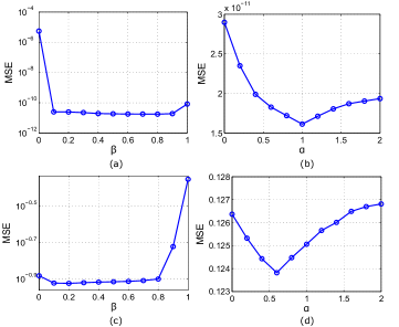
Figure 1: MSE performance of sensing matrices generated by Approach II with different values of $\alpha$ and $\beta$. (a) $\sigma^{2}=0,\ \alpha=1;$ (b) $\sigma^{2}=0,\ \beta=0.8;$ (c) $\sigma^{2}=10^{-2},\ \alpha=1;$ (d) $\sigma^{2}=10^{-2},\ \beta=0.2.$

Fig. 1 illustrates the results for the parameter tests. In Fig. 1 (a) and (c), the parameter $\beta$ is evaluated for the noiseless ($\sigma^{2}=0$) and high noise ($\sigma^{2}=10^{-2}$) cases, respectively, when $\alpha=1$. From both (a) and (c), we can see that when $\beta=0$ or 1, the MSE is larger than that for the other values, which means that both terms of Approach II that are controlled by $\beta$ are essential for obtaining optimal sensing matrices. In addition, we can see that when $\beta$ becomes larger in the range of $[0.1,\ 0.9]$, the MSE decreases slightly in (a), but increases slightly in (b). This indicates the choice of $\beta$ under different conditions of sensing noise, which is consistent with that observed in [20]. Thus in the remaining experiments, we take $\beta=0.8$ when sensing noise is low and $\beta=0.2$ when the noise is high. Fig. 1 (b) and (d) demonstrate the MSE results for the tests of parameter $\alpha$. It is observed that $\alpha=1$ is optimal for the noiseless case while it becomes $\alpha=0.6$ when high noise exists. Therefore a larger $\alpha$ is preferred when low noise is involved, which needs to be reduced accordingly when the noise becomes higher.

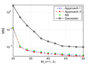
(a)

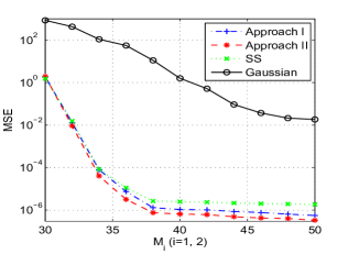
(b)

Figure 2: MSE performance of different sensing matrices for (a) the BP, (b) the OMP when $M_{i}\ (i=1,\ 2)$ varies. ($K=80,\ N_{1}=N_{2}=64,\ \hat{N}_{1}=\hat{N}_{2}=256$ and $\sigma^{2}=10^{-4}$)

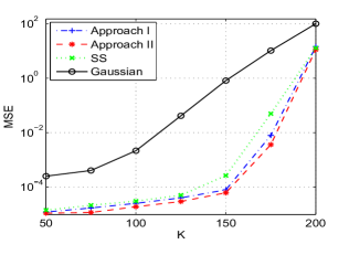
(a)

(b)

Figure 3: MSE performance of different sensing matrices for (a) the BP, (b) the OMP when $K$ varies. ($M_{1}=M_{2}=40,\ N_{1}=N_{2}=64,\ \hat{N}_{1}=\hat{N}_{2}=256$ and $\sigma^{2}=10^{-4}$)

We then proceed to examine the performance of both the proposed approaches. As this is the first work to optimize the multidimensional sensing matrix, we take the i.i.d Gaussian sensing matrices that are commonly used in CS problems for comparison. Besides, since Sapiro’s approach [18] has the same spirit to that of Approach I (as reviewed in Section III-A), it can be easily extended to the multidimensional case, i.e., individually generating $\boldsymbol{\Phi}_{i}\ (i=1,\ 2)$ using the approach in [18]. We hence also include it in the comparisons and denote it by Separable Sapiro’s approach (SS). The previously described synthetic data is generated for the experiments and both BP and OMP are investigated for the reconstruction.

Different sensing matrices are first evaluated using BP and OMP when the number of measurements varies. A small amount of noise ($\sigma^{2}=10^{-4}$) is added when taking measurements and the parameters are chosen as: $\alpha=1,\ \beta=0.8$. From Fig. 2, it can be observed that both the proposed approaches perform much better than the Gaussian sensing matrices, among which Approach II has better performance. In general, the SS method performs worse than Approach I, although the difference is not obvious at some points. Note that SS is an iterative method while Approach I is non-iterative.

The proposed approaches are again observed to be superior to the other methods when the number of measurements is fixed but the signal sparsity $K$ is varied, as shown in Fig. 3. Compared to Approach I, Approach II exhibits better performance, but at the cost of higher computational complexity and the proper choice of the parameters.

V-B Optimal Multidimensional Dictionary with the Sensing Matrices Coupled

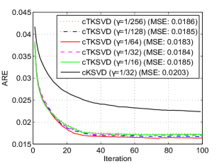
(a)

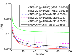
(b)

Figure 4: Convergence behavior of cTKSVD with different values of $\gamma$ compared to that of cKSVD with its optimal parameter setting when (a) $M_{1}=M_{2}=7;$ (b) $M_{1}=M_{2}=3$.

In this section, we evaluate the proposed cTKSVD method with a given multidimensional sensing matrix. A training sequence of 5000 2D signals ($T=5000$) is generated, i.e., $\underline{\mathbf{S}}\in\mathbb{R}^{18\times 18\times 5000}$, where each signal has $K=4\ (2\times 2)$ randomly placed non-zero elements that follow an i.i.d zero-mean unit-variance Gaussian distribution. The dictionaries $\boldsymbol{\Psi}_{i}\in\mathbb{R}^{10\times 18}\ (i=1,\ 2)$ are also drawn from i.i.d Gaussian distributions, followed by normalization such that they have unit-norm columns. The time-domain training signals $\underline{\mathbf{X}}\in\mathbb{R}^{10\times 10\times 5000}$ are then formed by: $\underline{\mathbf{X}}=\underline{\mathbf{S}}\times_{1}\boldsymbol{\Psi}_{1}\times_{2}\boldsymbol{\Psi}_{2}$. The test data of size $10\times 10\times 5000$ is generated following the same procedure. Random Gaussian noise with variance $\sigma^{2}$ is added to both the training and test data. Two i.i.d random Gaussian matrices are employed as the sensing matrices $\boldsymbol{\Phi}_{i}\in\mathbb{R}^{M_{i}\times 10}\ (i=1,\ 2)$, normalized by: $\boldsymbol{\Phi}_{i}=\sqrt{10}\boldsymbol{\Phi}_{i}/||\boldsymbol{\Phi}_{i}||_{F}.$ TOMP [29] is utilized in both the training stage and the reconstructions of the test stage for tensor-based approaches and OMP is employed for the vector-based approaches.

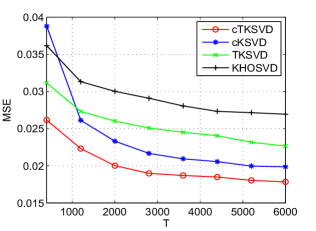
(a)

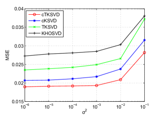
(b)

Figure 5: MSE performance of different dictionaries when (a) $T$ varies ($\sigma^{2}=0$), (b) $\sigma^{2}$ varies ($T=5000$). ($K=4,\ M_{1}=M_{2}=7,\ N_{1}=N_{2}=10,\ \hat{N}_{1}=\hat{N}_{2}=18$)

We first investigate the convergence behavior of the cTKSVD approach and examine the choice of the parameter $\gamma$. We define the Average Representation Error (ARE) [14, 19] of cTKSVD as: $\sqrt{||\underline{\mathbf{Z}}-\underline{\mathbf{S}}\times_{1}\mathbf{D}_{1}\times_{2}\mathbf{D}_{2}||_{F}^{2}/len(\underline{\mathbf{Z}})},$ where $\underline{\mathbf{Z}}$, $\mathbf{D}_{1}$ and $\mathbf{D}_{2}$ have the same definitions as in (33). Fig. 4 shows the AREs of cTKSVD at different numbers of iterations for different values of $\gamma$. The cKSVD method [18] (reviewed in Section III-A) is also tested and only the results of the optimal $\gamma$ are displayed in Fig. 4. Note that cKSVD learns a single dictionary $\boldsymbol{\Psi}\in\mathbb{R}^{100\times 324}$, rather than the separable multilinear dictionaries $\boldsymbol{\Psi}_{i}\in\mathbb{R}^{10\times 18}\ (i=1,\ 2)$. The ARE of cKSVD is thus modified accordingly as: $\sqrt{||\mathbf{Z}-\mathbf{D}\mathbf{S}||_{F}^{2}/len(\mathbf{Z})}$, in which the symbols follow the definitions in (28). From Fig. 4, it can be seen that cTKSVD exhibits stable convergence behavior with different parameters. It converges to a lowest ARE with $\gamma=1/64$ when $M_{i}=7$ and the optimal $\gamma$ is $1/128$ when $M_{i}=3$. The reconstruction MSE values are also shown in the legend, which are similar to each other but reveal the same optimal choice of $\gamma$ as described. Thus the optimal $\gamma$ is lower when the number of measurements decreases, which is consistent with the observation in [18]. In both experiments, cTKSVD with the optimal $\gamma$ outperforms cKSVD in terms of ARE and MSE.

Then the MSE performance of dictionaries learned by cTKSVD is compared with that of cKSVD [18] and KHOSVD [32] when the number of training sequences $T$ and the noise variance $\sigma^{2}$ vary. We use $\gamma=1/64$ for cTKSVD and $\gamma=1/32$ for cKSVD. To see the benefit of coupling sensing matrices, we also evaluate the uncoupled version of the proposed approach, i.e., TKSVD, in the experiments. The results can be found in Fig. 5. It is observable that cTKSVD outperforms all the other methods in terms of the reconstruction MSE. The sensing-matrix-coupled approaches (cKSVD and cTKSVD) are superior to the uncoupled approaches (TKSVD and KHOSVD). The TKSVD method leads to smaller MSE compared to KHOSVD, as it fully exploits the multidimensional structure. In addition, since cKSVD is not an approach that explicitly considers a multidimensional dictionary, it requires longer training sequences to learn the multilinear structure from the vectorized data. As seen in Fig. 5 (a), to achieve a MSE of 0.02, cTKSVD only needs 2000 training data; while approximately 6000 is required for the cKSVD approach. For the same reason, the performance of cKSVD degrades dramatically when the training data is less than 1000.

V-C TCS with Jointly Optimized Sensing Matrix and Dictionary

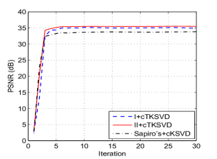
Figure 6: Convergence behavior of various joint optimization methods. ($T=5000,\ K=4,\ M_{1}=M_{2}=6,\ N_{1}=N_{2}=8,\ \hat{N}_{1}=\hat{N}_{2}=16,\ \sigma^{2}=0$)

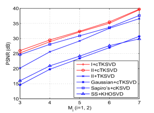
(a)

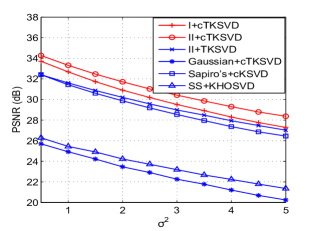
(b)

Figure 7: PSNR performance of different methods when (a) $M_{i}\ (i=1,\ 2)$ varies ($\sigma^{2}=0$), (b) $\sigma^{2}$ varies ($M_{1}=M_{2}=6$). ($T=5000,\ K=4,\ M_{1}=M_{2}=6,\ N_{1}=N_{2}=8,\ \hat{N}_{1}=\hat{N}_{2}=16$)

Now we examine the performance of the proposed joint optimization approach in Algorithm 3. The training data consists of 5000 $8\times 8$ patches obtained by randomly extracting 25 patches from each of the 200 images in a training set from the Berkeley segmentation dataset [46]. The test data is obtained by extracting non-overlapping $8\times 8$ patches from the other 100 images in the dataset. A 2D Discrete Cosine Transform (DCT) is employed to initialize the dictionaries $\boldsymbol{\Psi}_{i}\in\mathbb{R}^{8\times 16}\ (i=1,\ 2)$ and i.i.d Gaussian matrices are used as the initial sensing matrices $\boldsymbol{\Phi}_{i}\in\mathbb{R}^{M_{i}\times 8}\ (i=1,\ 2)$. Random Gaussian noise with variance $\sigma^{2}$ is added to the measurements at the test stage. We employ TOMP for reconstruction and the Peak Signal to Noise Ratio (PSNR) is used as the evaluation criteria.

In the first experiment, we examine the convergence behavior of Algorithm 3 when the proposed approach I and II are utilized for the sensing matrix optimization step (respectively denote by I + cTKSVD and II + cTKSVD). We take $M_{1}=M_{2}=6$ and no noise is added to the measurements at the test stage, i.e., $\sigma^{2}=0$. By conducting the simulations performed previously to obtain the results in Fig. 1 and 4, the parameters are chosen as: $\alpha=3,\ \beta=0.8,\ \gamma=1/8$. The step size for II + cTKSVD is set as: $\eta=1e-5$. The PSNR performance for different numbers of iterations is illustrated in Fig. 6. Since Sapiro’s approach in [18] also jointly optimizes the sensing matrix and dictionary, we include it in this figure (denoted by Sapiro’s + cKSVD). The parameter $\gamma$ is optimal at $1/2$ for cKSVD under our settings. However, note that Sapiro’s approach is only for vectorized signals in the conventional CS problem, i.e., a single sensing matrix $\boldsymbol{\Phi}\in\mathbb{R}^{36\times 64}$ and a dictionary $\boldsymbol{\Psi}\in\mathbb{R}^{64\times 256}$ are obtained. It is not suitable for a practical TCS system, where separable multidimensional sensing matrices $\boldsymbol{\Phi}_{i}\in\mathbb{R}^{6\times 8}\ (i=1,\ 2)$ are required. Even so, from Fig. 6, we can see the proposed approaches outperform Sapiro’s approach. All the methods converge in less than 10 iterations, among which II + cTKSVD leads to the highest PSNR value.

Then the proposed approaches are compared with various other approaches when the number of measurements ($M_{i}\ (i=1,\ 2)$) and the noise variance ($\sigma^{2}$) vary. Specifically, using the notation employed previously and by denoting the method of combining sensing matrix design with that of the dictionary learning using a “+”, the methods for comparison are: II + TKSVD, Gaussian + cTKSVD, Sapiro’s + cKSVD and SS + KHOSVD. In these approaches, II + TKSVD and SS + KHOSVD are uncoupled methods; Gaussian + cTKSVD does not involve sensing matrix optimization; Sapiro’s + cKSVD is for conventional CS system only.

The results are shown in Fig. 7. We can see that the proposed approaches obtain higher PSNR values than all of the other methods and II + cTKSVD performs best. To see the gain of coupling sensing matrices during dictionary learning and optimizing the sensing matrices, respectively, we compare II + cTKSVD with II + TKSVD and Gaussian + cTKSVD. For instance, when $M_{i}=5,\ \sigma^{2}=0$, II + cTKSVD has a gain of about 3dB over II + TKSVD and nearly 9dB over Gaussian + cTKSVD. Although Sapiro’s + cKSVD has a similar performance to ours at some specific settings, it is not for a TCS system that requires multiple separable sensing matrices. Examples of reconstructed images using these methods are demonstrated in Fig. 8 and 9 with the corresponding PSNR values listed. All of the conducted simulations verify that the proposed methods of multidimensional sensing matrix and dictionary optimization improve the performance of a TCS system.

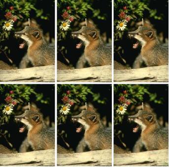
Figure 8: Reconstruction example when $M_{1}=M_{2}=6$. The images from left to right, top to bottom and their PSNR (dB) values are: II+cTKSVD (35.41), I+cTKSVD (34.97), Sapiro’s+cKSVD (33.64), II+TKSVD (33.57), SS+KHOSVD (28.62), Gaussian+cTKSVD (28.05).

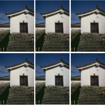
Figure 9: Reconstruction example when $M_{1}=M_{2}=4$. The images from left to right, top to bottom and their PSNR (dB) values are: II+cTKSVD (29.91), I+cTKSVD (29.45), Sapiro’s+cKSVD (28.72), II+TKSVD (26.60), SS+KHOSVD (22.62), Gaussian+cTKSVD (21.94).

VI Conclusions

In this paper, we propose to jointly optimize the multidimensional sensing matrix and dictionary for TCS systems. To obtain the optimized sensing matrices, a separable approach with closed form solutions has been presented and a joint iterative approach with novel design measures has also been proposed. The iterative approach certainly has higher complexity, but also exhibits better performance. An approach to learning the multidimensional dictionary has been designed, which explicitly takes the multidimensional structure into account and removes the redundant updates in the existing multilinear approaches in the literature. Further gain is obtained by coupling the multidimensional sensing matrix while learning the dictionary. The performance advantage of the proposed approaches has been demonstrated by experiments using both synthetic data and real images.

Appendix A Proof of Theorem 3

Assume $\mathbf{A}_{i}=\boldsymbol{\Phi}_{i}\boldsymbol{\Psi}_{i}=\mathbf{U}_{\mathbf{A}_{i}}\left[\begin{array}[]{cc}\boldsymbol{\Lambda}_{\mathbf{A}_{i}}&\mathbf{0}\end{array}\right]\mathbf{V}_{\mathbf{A}_{i}}^{T}$ is an SVD of $\mathbf{A}_{i}$ for $i=1,\ 2$ and $rank(\mathbf{A}_{i})=M_{i}$. Then the objective we want to minimize in (17) can be rewritten as:

$$\left|\left|\mathbf{I}_{\hat{N}_{1}\hat{N}_{2}}-(\mathbf{V}_{\mathbf{A}_{2}}\left[\begin{array}[]{cc}\boldsymbol{\Lambda}_{\mathbf{A}_{2}}^{2}&\mathbf{0}\\ \mathbf{0}&\mathbf{0}\end{array}\right]\mathbf{V}_{\mathbf{A}_{2}}^{T})\otimes(\mathbf{V}_{\mathbf{A}_{1}}\left[\begin{array}[]{cc}\boldsymbol{\Lambda}_{\mathbf{A}_{1}}^{2}&\mathbf{0}\\ \mathbf{0}&\mathbf{0}\end{array}\right]\mathbf{V}_{\mathbf{A}_{1}}^{T})\right|\right|{}_{F}^{2}.$$

Denote $\boldsymbol{\Sigma}=\left[\begin{array}[]{cc}\boldsymbol{\Lambda}_{\mathbf{A}_{2}}^{2}&\mathbf{0}\\ \mathbf{0}&\mathbf{0}\end{array}\right]\otimes\left[\begin{array}[]{cc}\boldsymbol{\Lambda}_{\mathbf{A}_{1}}^{2}&\mathbf{0}\\ \mathbf{0}&\mathbf{0}\end{array}\right]=diag(\boldsymbol{\nu}_{\mathbf{A}_{2}}\otimes\boldsymbol{\nu}_{\mathbf{A}_{1}}),$ $\boldsymbol{\nu}_{\mathbf{A}_{i}}=diag(\left[\begin{array}[]{cc}\boldsymbol{\Lambda}_{\mathbf{A}_{i}}^{2}&\mathbf{0}\\ \mathbf{0}&\mathbf{0}\end{array}\right])$, then we have

$$||\mathbf{I}_{\hat{N}_{1}\hat{N}_{2}}-(\mathbf{V}_{\mathbf{A}_{2}}\otimes\mathbf{V}_{\mathbf{A}_{1}})\boldsymbol{\Sigma}(\mathbf{V}_{\mathbf{A}_{2}}^{T}\otimes\mathbf{V}_{\mathbf{A}_{1}}^{T})||_{F}^{2}.$$ (68)

Let $\boldsymbol{\nu}_{\mathbf{A}_{i}}=[(v_{i})_{1},...,(v_{i})_{M_{i}},\mathbf{0}]^{T}$, then the sub-vector of the diagonal of $\boldsymbol{\Sigma}$ containing its non-zero values is: $\hat{\boldsymbol{\nu}}=[(v_{2})_{1}(v_{1})_{1},...,(v_{2})_{1}(v_{1})_{M_{1}},...,(v_{2})_{M_{2}}(v_{1})_{1},...,(v_{2})_{M_{2}}(v_{1})_{M_{1}}]^{T}$. Thus (68) becomes:

$$||\mathbf{I}_{\hat{N}_{1}\hat{N}_{2}}-\boldsymbol{\Sigma}||_{F}^{2}=\hat{N}_{1}\hat{N}_{2}-M_{1}M_{2}+\sum_{p=1}^{M_{2}}\sum_{q=1}^{M_{1}}(1-(v_{2})_{p}(v)_{q})^{2}.$$ (69)

Therefore we can obtain that the minimum value of (17) is $\hat{N}_{1}\hat{N}_{2}-M_{1}M_{2}$, and that it is achieved when the entries of $\hat{\boldsymbol{\nu}}$ are all unity.

Clearly $\boldsymbol{\Lambda}_{\mathbf{A}_{i}}$=$\mathbf{I}_{M_{i}}$ for $i=1,\ 2$ is a solution, i.e., $\mathbf{A}_{i}=\mathbf{U}_{\mathbf{A}_{i}}\left[\begin{array}[]{cc}\mathbf{I}_{M_{i}}&\mathbf{0}\end{array}\right]\mathbf{V}_{\mathbf{A}_{i}}^{T}$ with $\mathbf{U}_{\mathbf{A}_{i}}\in\mathbb{R}^{M_{i}\times M_{i}}$ and $\mathbf{V}_{\mathbf{A}_{i}}\in\mathbb{R}^{\hat{N}_{i}\times\hat{N}_{i}}$ being arbitrary orthonormal matrices. Then we would like to find $\boldsymbol{\Phi}_{i}\ (i=1,\ 2)$ such that $\boldsymbol{\Phi}_{i}\boldsymbol{\Psi}_{i}=\mathbf{U}_{\mathbf{A}_{i}}\left[\begin{array}[]{cc}\mathbf{I}_{M_{i}}&\mathbf{0}\end{array}\right]\mathbf{V}_{\mathbf{A}_{i}}^{T}$. Following the derivation of Theorem 2 in [11], the solution in (18) can be found.

With this solution, for an arbitrary vector $\mathbf{z}\in\mathbb{R}^{\hat{N}_{i}}$, we have $||\mathbf{A}_{i}^{T}\mathbf{z}||_{2}^{2}=tr(\mathbf{z}^{T}\mathbf{A}_{i}\mathbf{A}_{i}^{T}\mathbf{z})=tr(\mathbf{z}^{T}\mathbf{z})=||\mathbf{z}||_{2}^{2}$, which indicates that the resulting equivalent sensing matrices $\mathbf{A}_{i}\ (i=1,\ 2)$ are Parseval tight frames. In addition, we observe that the solution in (18) can be obtained by separately solving the sub-problems in (19), of which the solutions have been derived in [11]. By substituting the solutions of the sub-problems into (17), we can conclude the minimum remains as $\hat{N}_{1}\hat{N}_{2}-M_{1}M_{2}$.

References

- [1] E. J. Candes, J. Romberg, and T. Tao, “Robust uncertainty principles: exact signal reconstruction from highly incomplete frequency information,” IEEE Trans. Information Theory, Feb. 2006.
- [2] D. L. Donoho, “Compressed sensing,” IEEE Trans. Information Theory, April 2006.
- [3] E. J. Candès and M. B. Wakin, “An introduction to compressive sampling,” IEEE Signal Process. Magazine, vol. 25, no. 2, pp. 21 –30, March 2008.
- [4] M Lustig, D Donoho, and J Pauly., “Sparse MRI: The application of compressed sensing for rapid MR imaging,” Magn Reson Med, vol. 58, pp. 1182–1195, 2007.
- [5] W. Chen and I.J. Wassell, “Energy-efficient signal acquisition in wireless sensor networks: a compressive sensing framework,” IET Wireless Sensor Systems, vol. 2, no. 1, pp. 1–8, March 2012.
- [6] D. L. Donoho, M. Elad, and V. N. Temlyakov, “Stable recovery of sparse overcomplete representations in the presence of noise,” IEEE Trans. Information Theory, vol. 52, no. 1, pp. 6–18, 2006.
- [7] E. J. Candès, “The restricted isometry property and its implications for compressed sensing,” Comptes Rendus Mathematique, vol. 346, no. 9 - 10, pp. 589 – 592, 2008.
- [8] M. Elad, “Optimized projections for compressed sensing,” IEEE Trans. Signal Process., vol. 55, no. 12, pp. 5695–5702, 2007.
- [9] J. Xu, Y. Pi, and Z. Cao, “Optimized projection matrix for compressive sensing,” EURASIP J. on Advances in Signal Process., vol. 2010, pp. 43, 2010.
- [10] W. Chen, M. R. D Rodrigues, and I. Wassell, “Projection design for statistical compressive sensing: A tight frame based approach,” IEEE Trans. Signal Process., vol. 61, no. 8, pp. 2016–2029, 2013.
- [11] G. Li, Z. Zhu, D. Yang, L. Chang, and H. Bai, “On projection matrix optimization for compressive sensing systems,” IEEE Trans. Signal Process., vol. 61, no. 11, pp. 2887–2898, 2013.
- [12] N. Cleju, “Optimized projections for compressed sensing via rank-constrained nearest correlation matrix,” Applied. Comput. Harmonic Analysis, vol. 36, no. 3, pp. 495–507, 2014.
- [13] K. Engan, S. O. Aase, and J. H. Husøy, “Multi-frame compression: Theory and design,” EURASIP J. Signal Process., vol. 80, no. 10, pp. 2121–2140, 2000.
- [14] M. Aharon, M. Elad, and A. Bruckstein, “The KSVD: An algorithm for designing overcomplete dictionaries for sparse representation,” IEEE Trans. Signal Process., vol. 54, no. 11, pp. 4311–4322, 2006.
- [15] I. Tošić and P. Frossard, “Dictionary learning: What is the right representation for my signals,” IEEE Signal Process. Mag., vol. 28, no. 2, pp. 27–38, 2011.
- [16] S. K. Sahoo and A. Makur, “Dictionary training for sparse representation as generalization of K-means clustering,” IEEE Signal Process. Letters, vol. 20, no. 6, pp. 587–590, 2013.
- [17] W. Dai, T. Xu, and W. Wang, “Simultaneous codeword optimization (simco) for dictionary update and learning,” IEEE Trans. Signal Process., vol. 60, no. 12, pp. 6340–6353, 2012.
- [18] J. M. Duarte-Carvajalino and G. Sapiro, “Learning to sense sparse signals: Simultaneous sensing matrix and sparsifying dictionary optimization,” IEEE Trans. Image Process., vol. 18, no. 7, pp. 1395–1408, 2009.
- [19] W. Chen and M. R. D. Rodrigues, “Dictionary learning with optimized projection design for compressive sensing applications,” IEEE Signal Process. Letters, vol. 20, no. 10, pp. 992–995, 2013.
- [20] H. Bai, G. Li, S. Li, Q. Li, Q. Jiang, and L. Chang, “Alternating optimization of sensing matrix and sparsifying dictionary for compressed sensing,” IEEE Trans. Signal Process., vol. 63, no. 6, pp. 1581–1594, 2015.
- [21] B. Recht, M. Fazel, and P. A. Parrilo, “Guaranteed minimum-rank solutions of linear matrix equations via nuclear norm minimization,” SIAM Review, vol. 52, no. 3, pp. 471–501, 2010.
- [22] E. Candès and B. Recht, “Exact matrix completion via convex optimization,” Commun. ACM, vol. 55, no. 6, pp. 111–119, June 2012.
- [23] M. Golbabaee and P. Vandergheynst, “Compressed sensing of simultaneous low-rank and joint-sparse matrices,” arXiv, 2012.
- [24] R. Chartrand, “Nonconvex splitting for regularized low-rank+ sparse decomposition,” IEEE Trans. Signal Process., vol. 60, no. 11, pp. 5810–5819, 2012.
- [25] R. Otazo, E. Candès, and D. K. Sodickson, “Low-rank plus sparse matrix decomposition for accelerated dynamic mri with separation of background and dynamic components,” Mag. Res. in Medicine, vol. 73, no. 3, pp. 1125–1136, 2015.
- [26] M. F. Duarte and R. G. Baraniuk, “Kronecker compressive sensing,” IEEE Trans. Image Process., vol. 21, no. 2, pp. 494–504, Feb 2012.
- [27] N. D. Sidiropoulos and A. Kyrillidis, “Multi-way compressed sensing for sparse low-rank tensors,” IEEE Signal Process. Letters, vol. 19, no. 11, pp. 757–760, 2012.
- [28] S. Friedland, Q. Li, and D. Schonfeld, “Compressive sensing of sparse tensors,” IEEE Trans. Image Process., vol. 23, no. 10, pp. 4438–4447, Oct 2014.
- [29] C. F. Caiafa and A. Cichocki, “Multidimensional compressed sensing and their applications,” Wiley Interdisciplinary Reviews: Data Mining and Knowledge Discovery, vol. 3, no. 6, pp. 355–380, 2013.
- [30] C. F. Caiafa and A. Cichocki, “Computing sparse representations of multidimensional signals using kronecker bases,” Neural Comput., vol. 25, no. 1, pp. 186–220, Jan. 2013.
- [31] M. Seibert, J. Wormann, R. Gribonval, and M. Kleinsteuber, “Separable cosparse analysis operator learning,” in Proc. EUSIPCO, 2014, pp. 770–774.
- [32] F. Roemer, G. D. Galdo, and M. Haardt, “Tensor-based algorithms for learning multidimensional separable dictionaries,” in Proc. IEEE ICASSP, 2014, pp. 3963–3967.
- [33] Y. Peng, D. Meng, Z. Xu, C. Gao, Y. Yang, and B. Zhang, “Decomposable nonlocal tensor dictionary learning for multispectral image denoising,” in proc. IEEE CVPR, 2014, pp. 2949–2956.
- [34] M.F. Duarte, M.A. Davenport, D. Takhar, J.N. Laska, Ting Sun, K.F. Kelly, and R.G. Baraniuk, “Single-pixel imaging via compressive sampling,” IEEE Signal Process. Magazine, vol. 25, no. 2, pp. 83 –91, March 2008.
- [35] R. F. Marcia, Z. T. Harmany, and R. M. Willett, “Compressive coded aperture imaging,” SPIE 7246, Comput. Imag. VII, p. 72460G, 2009.
- [36] V. Majidzadeh, L. Jacques, A. Schmid, P. Vandergheynst, and Y. Leblebici, “A (256x256) pixel 76.7mW CMOS imager/ compressor based on real-time in-pixel compressive sensing,” in in Proc. IEEE ISCAS, June 2010, pp. 2956 –2959.
- [37] E.J. Candès and T. Tao, “Decoding by linear programming,” IEEE Trans. Information Theory, vol. 51, no. 12, pp. 4203 – 4215, Dec. 2005.
- [38] J.A. Tropp and A.C. Gilbert, “Signal recovery from random measurements via orthogonal matching pursuit,” IEEE Trans. Information Theory, vol. 53, no. 12, pp. 4655 –4666, Dec. 2007.
- [39] T. Blumensath and M. E. Davies, “Iterative hard thresholding for compressed sensing,” Applied and Computational Harmonic Analysis, vol. 27, no. 3, pp. 265–274, 2009.
- [40] Y. Rivenson and A. Stern, “Compressed imaging with a separable sensing operator,” IEEE Signal Process. Letters, vol. 16, no. 6, pp. 449–452, June 2009.
- [41] Y. Rivenson and A. Stern, “Practical compressive sensing of large images,” in Digital Signal Processing, 2009 16th International Conference on, July 2009, pp. 1–8.
- [42] W. Chen, M. R. D. Rodrigues, and I. J. Wassell, “On the use of unit-norm tight frames to improve the average mse performance in compressive sensing applications,” IEEE Signal Process. Letters, vol. 19, no. 1, pp. 8–11, 2012.
- [43] C. F. Van Loan, “The ubiquitous Kronecker product,” J. comput. applied mathematics, vol. 123, no. 1, pp. 85–100, 2000.
- [44] L. De Lathauwer, B. De Moor, and J. Vandewalle, “A multilinear singular value decomposition,” SIAM J. on Matrix Analysis. Applications., vol. 21, no. 4, pp. 1253–1278, 2000.
- [45] E. V. D. Berg and M. P. Friedlander, “Probing the pareto frontier for basis pursuit solutions,” SIAM Journal on Scientific Computing, vol. 31, no. 2, pp. 890–912, 2008.
- [46] D. Martin, C. Fowlkes, D. Tal, and J. Malik, “A database of human segmented natural images and its application to evaluating segmentation algorithms and measuring ecological statistics,” in Proc. IEEE ICCV, 2001, vol. 2, pp. 416–423.