Inference for Sparse and Dense Functional Data with Covariate Adjustments

Dominik Liebl
Institute for Financial Economics and Statistics, University of Bonn
Abstract

We consider inference for the mean and covariance functions of covariate adjusted functional data using Local Linear Kernel (LLK) estimators. By means of a double asymptotic, we differentiate between sparse and dense covariate adjusted functional data – depending on the relative order of $m$ (the discretization points per function) and $n$ (the number of functions). Our simulation results demonstrate that the existing asymptotic normality results can lead to severely misleading inferences in finite samples. We explain this phenomenon based on our theoretical results and propose finite-sample corrections which provide practically useful approximations for inference in sparse and dense data scenarios. The relevance of our theoretical results is showcased using a real-data application.


Keywords: functional data analysis, local linear kernel estimation, asymptotic normality, multiple bandwidth selection, finite-sample correction

1 Introduction

This work considers the case of independently identically distributed (iid) covariate adjusted functional data $X_{i}(.,Z_{i})\in L^{2}([0,1])$, $i=1,\dots,n$, with random covariate $Z_{i}\in[0,1]\subset\mathbb{R}$. As typically for longitudinal data, the single functions are only observed at error-prone measurements sampled at a certain number of random locations. That is, each unobserved random function $X_{i}(.,Z_{i})$ is observed at $m$ data points data points $(Y_{ij},U_{ij})\in\mathbb{R}^{2}$ with

$\displaystyle Y_{ij}$ $\displaystyle=X_{i}(U_{ij},Z_{i})+\epsilon_{ij},\quad j=1,\dots,m,\quad i=1,\dots,n,$ (1)

where $\epsilon_{ij}\in\mathbb{R}$ is an iid error term with mean zero and $\operatorname{\mathbb{V}}(\epsilon_{ij})=\sigma^{2}_{\epsilon}<\infty$ independent from $X_{i}$, $U_{ij}$, and $Z_{i}$.

We derive inferential results for the LLK estimators of the mean function $\mu(u,z)=\operatorname{\mathbb{E}}(X_{i}(u,z))$ and the covariance function $\gamma(u_{1},u_{2},z)=\operatorname{Cov}(X_{i}(u_{1},z),X_{i}(u_{2},z))$. So far the only other existing asymptotic normality results in this context are those of Jiang and Wang (2010), who consider the case of sparse covariate adjusted functional data, where sparse refers to the asymptotic scenario with $m$ being bounded while $n\to\infty$ (i.e., a finite-$m$ asymptotic). However, as shown in our simulation study, the asymptotic variance expressions derived in Jiang and Wang (2010) tend to severely underestimate the actual variances in finite samples. This can result in false inferences (size-distortion) in finite samples.

We are able to explain this finding based on our asymptotic normality results. The finite-$m$ asymptotic considered by Jiang and Wang (2010) neglects an additional functional-data-specific variance term which is typically not negligible in practice. In contrast to Jiang and Wang (2010), we consider sparse and dense functional data depending on the relative order of $m$ and $n$. This approach is related to the work of Zhang and Wang (2016), who, however, consider classical functional data without covariate adjustments111Our results are based on the author’s PhD thesis (Liebl, 2013) and were developed independently from the work of Zhang and Wang (2016)..

Additionally, we derive the explicit optimal multiple bandwidth expressions for the case of sparse and dense covariate adjusted functional data. For dense functional data, this leads to rather unconventional bandwidth expressions with different convergence rates for the bandwidths in $U$- and $Z$-direction. Effectively, this imposes a necessary under-smoothing in $U$-direction, which guarantees that the $U$-related bias and variance components become negligible in comparison to the $Z$-related bias and variance components.

Our third contribution is concerned with finite-samples. The differentiation between sparse and dense functional data is based on pure theoretical considerations. In practice, however, it is usually impossible to differentiate between these two asymptotic data scenarios. Therefore, we contribute finite-sample corrections that allow for robust inferences with sparse and dense functional data.

Generally, there are many different concepts of sparsity and we refer to Aneiros and Vieu (2016) for a comprehensive overview. Throughout this paper, we use the terms sparse and dense in order to differentiate between the following two asymptotic scenarios:

sparse: $m/n^{1/5}\to 0$ and dense: $m/n^{1/5}\to\infty$,

where the value $1/5$ of the exponent is determined by our theory. The sparse asymptotic scenario approximates cases where $m$ is relatively small in comparison to $n^{1/5}$, i.e., very small in comparison to $n$, and includes the finite-$m$ asymptotic of Jiang and Wang (2010). The dense asymptotic scenario approximates cases where $m$ is relatively large in comparison to $n^{1/5}$; however, not necessarily large in comparison to $n$. The terminology of sparse and dense asymptotic scenarios refers to the work of Zhang and Wang (2016).

The term dense, however, must be used with caution as it has the here misleading connotation of many data points $m$, which not necessarily applies to this asymptotic scenario222Indeed, Zhang and Wang (2016) use the term ultra-dense which has a potentially even more misleading connotation., since it includes cases where $m$ is relatively small in comparison to $n$, i.e., scenarios with possibly not so many data points $m$. Indeed, for large $m$ it is usually advantageous to pre-smooth the single functions and to neglect the pre-smoothing error (Zhang and Chen, 2007). In this paper, we focus on cases where the pre-smoothing approach cannot be applied due to a too small $m$.

The literature on covariate adjusted functional data was initiated by the work of Cardot (2007), who considers functional principal component analysis for dense functional data, but does not provide inferential results. Jiang and Wang (2010) focus on the case of sparse functional data. Li et al. (2015) consider a copula-based model and Zhang and Wei (2015) propose an iterative algorithm for computing functional principal components, though neither provides inferential results for the covariate adjusted mean and covariance functions. For the case without covariate adjustments there are several papers considering inference. Zhang and Chen (2007) and Hall and Van Keilegom (2007) consider inference in the pre-smoothing context for dense functional data. Ferraty et al. (2007), Ferraty et al. (2010), and Rana et al. (2016) consider inference in functional nonparametric regression. Benko et al. (2009) develop bootstrap procedures for the case of dense functional data. Cao et al. (2012) derive simultaneous confidence bands in the case of dense functional data. Gromenko and Kokoszka (2012) consider an $L^{2}$-based test statistic and address computational issues in finite samples and Horváth et al. (2013) focus on the case of dependent functional data within the same framework. Although related, the case without covariate adjustments is fundamentally different from our case, since the presence of a covariate affects the involved bandwidth selection problem in a nontrivial manner. Readers with a general interest in functional data analysis are referred to the textbooks of Ramsay and Silverman (2005), Ferraty and Vieu (2006), Horváth and Kokoszka (2012), Hsing and Eubank (2015), and Kokoszka and Reimherr (2017). Recent surveys of methodological advances in functional data analyses can be found in Cuevas (2014), Goia and Vieu (2016), and Wang et al. (2016).

The rest of this paper is structured as following. The next section introduces the considered regression models and LLK estimators. Section 3 presents our assumptions and asymptotic results. Our simulation study is in Section 4. Section 5 introduces rule-of-thumb approximations to our theoretical bandwidth expressions and practical plug-in estimates for the unknown bias and variance components. Section 6 contains our real data application. All proofs can be found in the appendix.

2 Nonparametric regression models and estimators

Let $X^{c}_{i}$ denote the centered random function $X^{c}_{i}(U_{ij},Z_{i})=X_{i}(U_{ij},Z_{i})-\operatorname{\mathbb{E}}(X_{i}(U_{ij},Z_{i})|\mathbf{U},\mathbf{Z})$, where $\mathbf{U}=(U_{11},\dots,U_{nm})^{\top}$ and $\mathbf{Z}=(Z_{1},\dots,Z_{n})^{\top}$. Model (1) can be written as a nonparametric regression model with the bivariate mean function $\mu(U_{ij},Z_{i})=\operatorname{\mathbb{E}}(X_{i}(U_{ij},Z_{i})|\mathbf{U},\mathbf{Z})$ as the regression function,

$\displaystyle Y_{ij}=\mu(U_{ij},Z_{i})+X^{c}_{i}(U_{ij},Z_{i})+\epsilon_{ij},\quad i=1,\dots,n,\quad j=1,\dots,m,$ (2)

where $X^{c}_{i}(.,z)\in L^{2}[0,1]$ is an iid centered random function, $U_{ij}\in[0,1]$ and $Z_{i}\in[0,1]$ are iid random predictors, and $\epsilon_{ij}\in\mathbb{R}$ is an iid random error term independent from $X_{i}^{c}$, $U_{ij}$ and $Z_{i}$. Note that Model (2) has a rather unusual composed error term $X^{c}_{i}(U_{ij},Z_{i})+\epsilon_{ij}$ consisting of a function- and a scalar-valued component. This structure of the error term leads to an additional functional-data-specific variance term.

Likewise to Model (2) we can define the following nonparametric regression model with the trivariate covariance function $\gamma(U_{ij},U_{ik},Z_{i})=\operatorname{Cov}(X_{i}(U_{ij},Z_{i}),X_{i}(U_{ik},Z_{i})|\mathbf{U},\mathbf{Z})$ as the regression function:

$\displaystyle C_{ijk}$ $\displaystyle=\gamma(U_{ij},U_{ik},Z_{i})+\tilde{X}^{c}_{i}(U_{ij},U_{ik},Z_{i})+\varepsilon_{ijk},\quad i=1,\dots,n,\quad j\neq k\in\{1,\dots,m\},$ (3)

where the raw-covariances $C_{ijk}$, the centered random function $\tilde{X}^{c}_{i}$, and the scalar-valued error term $\varepsilon_{ijk}$ are defined as

$\displaystyle C_{ijk}$ $\displaystyle=(Y_{ij}-\mu(U_{ij},Z_{i}))(Y_{ik}-\mu(U_{ik},Z_{i})),$ (4)
$\displaystyle\tilde{X}^{c}_{i}(U_{ij},U_{ik},Z_{i})$ $\displaystyle=X^{c}_{i}(U_{ij},Z_{i})\,X^{c}_{i}(U_{ik},Z_{i})-\gamma(U_{ij},U_{ik},Z_{i}),\;\text{and}$
$\displaystyle\varepsilon_{ijk}$ $\displaystyle=X^{c}_{i}(U_{ij},Z_{i})\epsilon_{ik}+X^{c}_{i}(U_{ik},Z_{i})\epsilon_{ij}+\epsilon_{ij}\epsilon_{ik}.$

In contrast to $\epsilon_{ij}$, the scalar error term $\varepsilon_{ijk}$ is heteroscedastic with $\operatorname{\mathbb{V}}(\varepsilon_{ijk})=\sigma^{2}_{\varepsilon}(u_{1},u_{2},z)$, where $\sigma^{2}_{\varepsilon}(u_{1},u_{2},z)=\gamma(u_{1},u_{1},z)\,\sigma^{2}_{\epsilon}+\gamma(u_{2},u_{2},z)\sigma^{2}_{\epsilon}+\sigma^{4}_{\epsilon}$. Note that $\operatorname{\mathbb{E}}(\varepsilon_{ijk})\neq 0$ for all $j=k$, therefore all raw covariance points $C_{ijk}$ with $j=k$ need to be excluded (see also Yao et al., 2005). Correspondingly, the number of raw covariance points for each $i$ is $M=m^{2}-m$, which makes it necessary that $m\geq 2$. As in Model (2), the error term of Model (3), $\tilde{X}^{c}_{i}(U_{ij},U_{ik},Z_{i})+\varepsilon_{ijk}$, consists of a function- and a scalar-valued component.

We estimate the mean function $\mu(u,z)$ using the LLK estimator $\hat{\mu}(u,z;h_{\mu,U},h_{\mu,Z})$ defined as the following locally weighted least squares estimator (see, e.g., Ruppert and Wand, 1994):

$\displaystyle\hat{\mu}(u,z;h_{\mu,U},h_{\mu,Z})=e_{1}^{\top}\left([\mathbf{1},\mathbf{U}_{u},\mathbf{Z}_{z}]^{\top}\mathbf{W}_{\mu,uz}[\mathbf{1},\mathbf{U}_{u},\mathbf{Z}_{z}]\right)^{-1}[\mathbf{1},\mathbf{U}_{u},\mathbf{Z}_{z}]^{\top}\mathbf{W}_{\mu,uz}\mathbf{Y},$ (5)

where the vector $e_{1}=(1,0,0)^{\top}$ selects the estimated intercept parameter and $[\mathbf{1},\mathbf{U}_{u},\mathbf{Z}_{z}]$ is a partitioned $nm\times 3$ dimensional data matrix with typical rows $(1,U_{ij}-u,Z_{i}-z)$. The $nm\times nm$ dimensional diagonal weighting matrix $\mathbf{W}_{\mu,uz}$ holds the bivariate multiplicative kernel weights $K_{\mu,h_{\mu,U},h_{\mu,Z}}(U_{ij}-u,Z_{i}-z)=h^{-1}_{\mu,U}\,\kappa(h^{-1}_{\mu,U}(U_{ij}-u))\;h^{-1}_{\mu,Z}\,\kappa(h^{-1}_{\mu,Z}(Z_{i}-z)),$ where $\kappa$ is a usual second-order kernel such as, e.g., the Epanechnikov or the Gaussian kernel. The usual kernel constants are denoted by $\nu_{2}(K_{\mu})=\left(\nu_{2}(\kappa)\right)^{2}$, with $\nu_{2}(\kappa)=\int u^{2}\kappa(u)du$, and $R(K_{\mu})=R(\kappa)^{2}$, with $R(\kappa)=\int\kappa(u)^{2}du$. All vectors and matrices are filled in correspondence with the $nm$ dimensional vector $\mathbf{Y}=(Y_{11},Y_{12},\dots,Y_{n,m-1},Y_{n,m})^{\top}$.

The LLK estimator for the covariance function $\gamma(u_{1},u_{2},z)$ is defined correspondingly as

$\displaystyle\begin{split}&\hat{\gamma}(u_{1},u_{2},z;h_{\gamma,U},h_{\gamma,Z})=\\ &=e_{1}^{\top}\left([\mathbf{1},\mathbf{U}_{u_{1}},\mathbf{U}_{u_{2}},\mathbf{Z}_{z}]^{\top}\mathbf{W}_{\gamma,u_{1}u_{2}z}[\mathbf{1},\mathbf{U}_{u_{1}},\mathbf{U}_{u_{2}},\mathbf{Z}_{z}]\right)^{-1}[\mathbf{1},\mathbf{U}_{u_{1}},\mathbf{U}_{u_{2}},\mathbf{Z}_{z}]^{\top}\mathbf{W}_{\gamma,u_{1}u_{2}z}\mathbf{C},\end{split}$ (6)

where $e_{1}=(1,0,0,0)^{\top}$ and $[\mathbf{1},\mathbf{U}_{u_{1}},\mathbf{U}_{u_{2}},\mathbf{Z}_{z}]$ is a $nM\times 4$ dimensional data matrix with typical rows $(1,U_{ij}-u_{1},U_{ik}-u_{2},Z_{i}-z)$. The $nM\times nM$ dimensional diagonal weighting matrix $\mathbf{W}_{\gamma,u_{1}u_{2}z}$ holds the trivariate multiplicative kernel weights $K_{\gamma,h_{\gamma,U},h_{\gamma,Z}}(U_{ij}-u_{1},U_{ik}-u_{2},Z_{i}-z)=h^{-1}_{\gamma,U}\,\kappa(h^{-1}_{\gamma,U}(U_{ij}-u_{1}))\;h^{-1}_{\gamma,U}\,\kappa(h^{-1}_{\gamma,U}(U_{ik}-u_{2}))\;h^{-1}_{\gamma,Z}\,\kappa(h^{-1}_{\gamma,Z}(Z_{i}-z))$, where $\kappa$ is as defined above, with kernel constants are $\nu_{2}(K_{\gamma})=\left(\nu_{2}(\kappa)\right)^{3}$ and $R(K_{\gamma})=R(\kappa)^{3}$. All vectors and matrices are filled in correspondence with the $nM$ dimensional vector $\mathbf{C}=(C_{112},C_{113},\dots,C_{n,m,m-2},C_{n,m,m-1})^{\top}$, where

$$\hat{C}_{ijk}=(Y_{ij}-\hat{\mu}(U_{ij},Z_{i};h_{\mu,U},h_{\mu,Z}))(Y_{ik}-\hat{\mu}(U_{ik},Z_{i};h_{\mu,U},h_{\mu,Z})).$$

3 Theoretical results

Before we present our asymptotic results, we list our additional assumptions which are equivalent to those in Ruppert and Wand (1994) with some straight forward adjustments to our functional data context.


A-AS (Asymptotic Scenario) $nm\to\infty$, where $m=m_{n}\geq 2$ such that $m_{n}\asymp n^{\theta}$ with $0\leq\theta<\infty$. Here, $m_{n}\asymp n^{\theta}$ denotes that the two sequences $m_{n}$ and $n^{\theta}$ are asymptotically equivalent, i.e., that $0<\lim_{n\rightarrow\infty}(m_{n}/n^{\theta})<\infty$.


A-RD (Random Design) The triple $(Y_{ij},U_{ij},Z_{i})\in\mathbb{R}\times[0,1]^{2}$ has the same distribution as $(Y,U,Z)$ with pdf $f_{YUZ}$, where $f_{YUZ}(y,u,z)>0$ for all $(y,u,z)\in\mathbb{R}\times[0,1]^{2}$ and zero else. Equivalently, $(C_{ijk},U_{ij},U_{ik},Z_{i})\in\mathbb{R}\times[0,1]^{3}$ has the same distribution as $(C,U,U^{\prime},Z)$ with pdf $f_{CUUZ}$, where $f_{CUUZ}(c,u,u^{\prime},z)>0$ for all $(c,u,u^{\prime},z)\in\mathbb{R}\times[0,1]^{3}$ and zero else.


A-SK (Smoothness & Kernel) The pdfs $f_{YUZ}$ and $f_{CUUZ}$ and their marginals are continuously differentiable. All second-order derivatives of $\mu$ and $\gamma$ are continuous. The multiplicative kernel functions $K_{\mu}$ and $K_{\gamma}$ are products of second-order kernel functions $\kappa$.


A-MO (Moments) $\operatorname{\mathbb{E}}((X_{i}(u,z))^{4})<\infty$ for all $(u,z)$ and $\operatorname{\mathbb{E}}(\epsilon_{ij}^{2})<\infty$.


A-BW (Bandwidths) $h_{\mu,U},h_{\mu,Z}\to 0$ and $(nm)h_{\mu,U}h_{\mu,Z}\to\infty$ as $nm\to\infty$. $h_{\mu,U},h_{\mu,Z}\to 0$ and $(nM)h_{\mu,U}^{2}h_{\mu,Z}\to\infty$ as $nM\to\infty$.

Remark

Assumption A-AS is a simplified version of the asymptotic setup of Zhang and Wang (2016). The case $\theta=0$ implies that $m$ is bounded, which corresponds to the finite-$m$ asymptotic as considered by Jiang and Wang (2010). For $0<\theta<\infty$ we can consider also sparse and dense functional data. As typically done in multivariate nonparametric regressions, we focus on the case of bounded random regressors $U_{ij}$ and $Z_{i}$. The case of unbounded regressors is beyond the scope of this paper, but may be adapted from Hansen (2008), who considers, however, a much simplex context.

The following two Theorems 3.1 and 3.2 build the basis of our theoretical results.

Theorem 3.1 (Bias and Variance of $\hat{\mu}$)

Let $(u,z)$ be an interior point of $[0,1]^{2}$. Under our setup the conditional asymptotic bias and variance of the LLK estimator in Eq. (5) are then given by

$\displaystyle\text{{(i)}}\operatorname{Bias}\left\{\hat{\mu}(u,z;h_{\mu,U},h_{\mu,Z})|\mathbf{U},\mathbf{Z}\right\}=B_{\mu}(u,z)\left(1+o_{p}(1)\right)\text{ with}\hskip 85.35826pt$
$\displaystyle B_{\mu}(u,z)=\frac{1}{2}\;\nu_{2}(K_{\mu})\,\left(h^{2}_{\mu,U}\,\mu^{(2,0)}(u,z)+h^{2}_{\mu,Z}\,\mu^{(0,2)}(u,z)\right),$
$\displaystyle\text{where }\mu^{(k,l)}(u,z)=(\partial^{k+l}/(\partial u^{k}\partial z^{l}))\mu(u,z).$
$\displaystyle\text{{(ii)} }\operatorname{\mathbb{V}}\left\{\hat{\mu}(u,z;h_{\mu,U},h_{\mu,Z})|\mathbf{U},\mathbf{Z}\right\}=\left(V_{\mu}^{I}(u,z)+V_{\mu}^{II}(u,z)\right)\left(1+o_{p}(1)\right)\text{ with}$
$\displaystyle V_{\mu}^{I}(u,z)=(nm)^{-1}\left[h_{\mu,U}^{-1}h_{\mu,Z}^{-1}\,R(K_{\mu})\frac{\gamma(u,u,z)+\sigma^{2}_{\epsilon}}{f_{UZ}(u,z)}\,\right]\text{ and}$
$\displaystyle V_{\mu}^{II}(u,z)=n^{-1}\left[\left(\frac{m-1}{m}\right)h_{\mu,Z}^{-1}\,R(\kappa)\frac{\gamma(u,u,z)}{f_{Z}(z)}\right].$
Theorem 3.2 (Bias and Variance of $\hat{\gamma}$)

Let $(u_{1},u_{2},z)$ be an interior point of $[0,1]^{3}$. Under our setup the conditional asymptotic bias and variance of the LLK estimator in Eq. (6) are then given by

$\displaystyle\text{{(i)}}\operatorname{Bias}\left\{\hat{\gamma}(u_{1},u_{2},z;h_{\gamma,U},h_{\gamma,Z})|\mathbf{U},\mathbf{Z}\right\}=B_{\gamma}(u_{1},u_{2},z)\left(1+o_{p}(1)\right)\text{ with}$
$\displaystyle B_{\gamma}(u_{1},u_{2},z)=\frac{1}{2}\nu_{2}(K_{\gamma})\left(h^{2}_{\gamma,U}\left(\gamma^{(2,0,0)}(u_{1},u_{2},z)+\gamma^{(0,2,0)}(u_{1},u_{2},z)\right)+h^{2}_{\gamma,Z}\gamma^{(0,0,2)}(u_{1},u_{2},z)\right),$
$\displaystyle\text{where }\gamma^{(k,l,m)}(u_{1},u_{2},z)=(\partial^{k+l+m}/(\partial u_{1}^{k}\,\partial u_{2}^{l}\,\partial z^{m}))\gamma(u_{1},u_{2},z).$
$\displaystyle\text{{(ii)} }\operatorname{\mathbb{V}}\left\{\hat{\gamma}(u_{1},u_{2},z;h_{\gamma,U},h_{\gamma,Z})|\mathbf{U},\mathbf{Z}\right\}=\left(V_{\gamma}^{I}(u_{1},u_{2},z)+V_{\gamma}^{II}(u_{1},u_{2},z)\right)\left(1+o_{p}(1)\right)\text{with}$
$\displaystyle V_{\gamma}^{I}(u_{1},u_{2},z)=(nM)^{-1}\left[h_{\gamma,U}^{-2}h_{\gamma,Z}^{-1}\,R(K_{\gamma})\frac{\tilde{\gamma}((u_{1},u_{2}),(u_{1},u_{2}),z)+\sigma^{2}_{\varepsilon}(u_{1},u_{2},z)}{f_{UUZ}(u_{1},u_{2},z)}\,\right]\text{and}$
$\displaystyle V_{\gamma}^{II}(u_{1},u_{2},z)=n^{-1}\left[\left(\frac{M-1}{M}\right)h_{\gamma,Z}^{-1}\,R(\kappa)\frac{\tilde{\gamma}((u_{1},u_{2}),(u_{1},u_{2}),z)}{f_{Z}(z)}\right],$
$$\begin{array}[]{rcl}\text{where}\quad\tilde{\gamma}((u_{1},u_{2}),(u_{1},u_{2}),z)&=&\operatorname{Cov}(\tilde{X}^{c}_{i}(u_{1},u_{2},z),\tilde{X}^{c}_{i}(u_{1},u_{2},z))\quad\text{and}\\ \sigma^{2}_{\varepsilon}(u_{1},u_{2},z)&=&\gamma(u_{1},u_{1},z)\,\sigma^{2}_{\epsilon}+\gamma(u_{2},u_{2},z)\sigma^{2}_{\epsilon}+\sigma^{4}_{\epsilon}.\end{array}$$

The bias expressions in Theorems 3.1 and 3.2 correspond to the classical bias results (see, e.g., Ruppert and Wand, 1994). The first variance terms $V_{\mu}^{I}(u,z)$ and $V_{\gamma}^{I}(u_{1},u_{2},z)$ are equivalent to those in Theorems 3.2 and 3.4 of Jiang and Wang (2010) who consider the LLK estimators $\hat{\mu}(u,z)$ and $\hat{\gamma}(u,z)$ under the finite-$m$ asymptotic. The second functional-data-specific variance terms, $V_{\mu}^{II}(u,z)$ and $V_{\gamma}^{II}(u_{1},u_{2},z)$, are negligible under such a finite-$m$ asymptotic, but generally not negligible when considering a double asymptotic where both $m\to\infty$ and $n\to\infty$.

Whether the first variance terms, $V_{\mu}^{I}$ and $V_{\gamma}^{I}$, or the second, functional-data-specific variance terms, $V_{\mu}^{II}$ and $V_{\gamma}^{II}$, are the leading variance terms depends on the bandwidth choices and on the relative order of $m$ and $n$, i.e., on the value of $\theta$ in $m\asymp n^{\theta}$. In order to determine the decisive $\theta$ value we postulate optimal bandwidth choices determined from minimizing the usual Asymptotic Mean Integrated Squared Error (AMISE) criteria,

$$\begin{array}[]{l}\operatorname{AMISE}_{\hat{\mu}}=\int\big{(}[\operatorname{Bias}\{\hat{\mu}(u,z)|\mathbf{U},\mathbf{Z}\}]^{2}+\operatorname{\mathbb{V}}\{\hat{\mu}(u,z)|\mathbf{U},\mathbf{Z}\}\big{)}f_{UZ}(u,z)\,d(u,z)\quad\text{and}\\[7.74997pt] \operatorname{AMISE}_{\hat{\gamma}}=\int\big{(}[\operatorname{Bias}\{\hat{\gamma}(u_{1},u_{2},z)|\mathbf{U},\mathbf{Z}\}]^{2}+\operatorname{\mathbb{V}}\{\hat{\gamma}(u_{1},u_{2},z)|\mathbf{U},\mathbf{Z}\}\big{)}f_{UUZ}(u_{1},u_{2},z)\,d(u_{1},u_{2},z).\\[-2.84526pt] \end{array}$$

In anticipation of some of our results: Under AMISE optimal bandwidth choices, the discriminating $\theta$-threshold is given by $\theta=1/5$. That is, if $m/n^{1/5}\to 0$ and $\sqrt{M}/n^{1/5}\to 0$, the first variance terms $V_{\mu}^{I}$ and $V_{\gamma}^{I}$ are the leading variance terms. This asymptotic scenario comprises situations where $m$ and $\sqrt{M}$ are eventually small in comparison to $n^{1/5}$, i.e., very small in comparison to $n$. Following Zhang and Wang (2016), we refer to this asymptotic scenario as sparse covariate adjusted functional data.

If, however, $m/n^{1/5}\to\infty$ and $\sqrt{M}/n^{1/5}\to\infty$, then the functional-data-specific variance terms $V_{\mu}^{II}$ and $V_{\gamma}^{II}$ are the leading variance terms. This asymptotic scenario comprises quite general situations where $m$ and $\sqrt{M}$ are eventually large in comparison to $n^{1/5}$, but not necessarily large in comparison to $n$. Following Zhang and Wang (2016), we refer to this asymptotic scenario as dense covariate adjusted functional data. However, we refer the reader to our cautionary note of the introduction as the term dense might have a misleading connotation.

Our theoretical results assume a homoscedastic variance $\sigma^{2}_{\epsilon}$ for the error term $\epsilon_{ij}$. In case of a heteroscedastic variance, one needs to replace the quantity $\sigma^{2}_{\epsilon}$ in Theorems 3.1 and 3.2 by, its heteroscedastic counterpart $\sigma^{2}_{\epsilon}(u,z)$. The unknown $\sigma^{2}_{\epsilon}(u,z)$ must then be estimated using a heteroscedasticity-consistent estimator.

3.1 Sparse functional data

The explicit AMISE optimal bandwidth expressions for the case of leading first variance terms, $V_{\mu}^{I}$ and $V_{\gamma}^{I}$, can be found in the following two Theorems:

Theorem 3.3 (Sparse - optimal bandwidths for $\hat{\mu}$)

Let $m/n^{1/5}\to 0$ and $(u,z)$ be an interior point of $[0,1]^{2}$. Under our setup the AMISE optimal bandwidths for the LLK estimator in Eq. (5) are then given by

$\displaystyle h^{S}_{\mu,U}$ $\displaystyle=\left(\frac{R(K_{\mu})\,Q_{\mu,1}\,\mathcal{I}_{\mu,ZZ}^{3/4}}{nm\,\left(\nu_{2}(K_{\mu})\right)^{2}\,\left[\mathcal{I}_{\mu,UU}^{1/2}\,\mathcal{I}_{\mu,ZZ}^{1/2}+\mathcal{I}_{\mu,UZ}\right]\mathcal{I}_{\mu,UU}^{3/4}}\right)^{1/6}$ (7)
$\displaystyle h^{S}_{\mu,Z}$ $\displaystyle=\left(\frac{\mathcal{I}_{\mu,UU}}{\mathcal{I}_{\mu,ZZ}}\right)^{1/4}h^{S}_{\mu,U},\text{ where}$ (8)
$$\begin{array}[]{l}Q_{\mu,1}=\int\left(\gamma(u,u,z)+\sigma^{2}_{\epsilon}\right)\,d(u,z),\;\;\mathcal{I}_{\mu,UZ}=\int\mu^{(2,0)}(u,z)\mu^{(0,2)}(u,z)\,f_{UZ}(u,z)\,d(u,z),\\ \mathcal{I}_{\mu,UU}=\int\left(\mu^{(2,0)}(u,z)\right)^{2}\,f_{UZ}(u,z)\,d(u,z),\,\text{and}\;\;\mathcal{I}_{\mu,ZZ}=\int\left(\mu^{(0,2)}(u,z)\right)^{2}\,f_{UZ}(u,z)\,d(u,z).\end{array}$$
Theorem 3.4 (Sparse - optimal bandwidths for $\hat{\gamma}$)

Let $\sqrt{M}/n^{1/5}\to 0$ and $(u_{1},u_{2},z)$ be an interior point of $[0,1]^{3}$. Under our setup the AMISE optimal bandwidths for the LLK estimator in Eq. (6) are then given by

$\displaystyle h^{S}_{\gamma,U}$ $\displaystyle=\left(\frac{R(K_{\gamma})\;Q_{\gamma,1}\;4\;\sqrt{2}\;\mathcal{I}_{\gamma,ZZ}^{3/2}}{nM\,\left(\nu_{2}(K_{\gamma})\right)^{2}\,\left(2\,\left(\nu_{2}(K_{\gamma})\right)^{2}\,\mathcal{I}_{\gamma,U_{(1)}Z}+C_{\mathcal{I}}\right)\,\left(C_{\mathcal{I}}-\mathcal{I}_{\gamma,U_{(1)}Z}\right)^{3/2}}\right)^{1/7}$ (9)
$\displaystyle h^{S}_{\gamma,Z}$ $\displaystyle=\left(\frac{C_{\mathcal{I}}-\mathcal{I}_{\gamma,U_{(1)}Z}}{2\,\mathcal{I}_{\gamma,ZZ}}\right)^{1/2}h^{S}_{\gamma,U},$ (10)
$$\begin{array}[]{rcl}\text{where \quad}C_{\mathcal{I}}&=&(\mathcal{I}_{\gamma,U_{(1)}Z}^{2}+4\,(\mathcal{I}_{\gamma,U_{(1)}U_{(1)}}+\mathcal{I}_{\gamma,U_{(1)}U_{(2)}})\,\mathcal{I}_{\gamma,ZZ})^{1/2},\\ Q_{\gamma,1}&=&\int\left(\tilde{\gamma}((u_{1},u_{2}),(u_{1},u_{2}),z)+\sigma^{2}_{\varepsilon}(u_{1},u_{2},z)\right)\,d(u_{1},u_{2},z)\\ \mathcal{I}_{\gamma,U_{(1)}U_{(1)}}&=&\int\left(\gamma^{(2,0,0)}(u_{1},u_{2},z)\right)^{2}\,f_{UUZ}(u_{1},u_{2},z)\,d(u_{1},u_{2},z),\\ \mathcal{I}_{\gamma,U_{(1)}U_{(2)}}&=&\int\left(\gamma^{(2,0,0)}(u_{1},u_{2},z)\gamma^{(0,2,0)}(u_{1},u_{2},z)\right)\,f_{UUZ}(u_{1},u_{2},z)\,d(u_{1},u_{2},z),\\ \mathcal{I}_{\gamma,U_{(1)}Z}&=&\int\gamma^{(2,0,0)}(u_{1},u_{2},z)\gamma^{(0,0,2)}(u_{1},u_{2},z)\,f_{UUZ}(u_{1},u_{2},z)\,d(u_{1},u_{2},z),\quad\text{and}\\ \mathcal{I}_{\gamma,ZZ}&=&\int\left(\gamma^{(0,0,2)}(u_{1},u_{2},z)\right)^{2}\,f_{UUZ}(u_{1},u_{2},z)\,d(u_{1},u_{2},z).\end{array}$$

The bandwidth rates are well-known for bi- and trivariate nonparametric estimators and essentially equivalent results can be found, e.g., in Herrmann et al. (1995). The superscript S stands for sparse covariate adjusted functional data.

The following Corollaries 3.1 and 3.2 contain our asymptotic normality results for the estimators $\hat{\mu}$ and $\hat{\gamma}$ for sparse functional data.

Corollary 3.1 (Sparse - asymptotic normality of $\hat{\mu}$)

Let $m/n^{1/5}\to 0$, let $(u,z)$ be an interior point of $[0,1]^{2}$, and assume optimal bandwidth choices. Under our setup the LLK estimator in Eq. (5) is then asymptotically normal.
(a) Without finite sample correction:

$\displaystyle\left(\frac{\hat{\mu}(u,z;h_{\mu,U}^{S},h_{\mu,Z}^{S})-B_{\mu}(u,z;h_{\mu,U}^{S},h_{\mu,Z}^{S})-\mu(u,z)}{\sqrt{V_{\mu}^{I}(u,z;h_{\mu,U}^{S},h_{\mu,Z}^{S})}}\right)\overset{a}{\sim}N(0,1)$

(b) With finite sample correction:

$\displaystyle\left(\frac{\hat{\mu}(u,z;h_{\mu,U}^{S},h_{\mu,Z}^{S})-B_{\mu}(u,z;h_{\mu,U}^{S},h_{\mu,Z}^{S})-\mu(u,z)}{\sqrt{V_{\mu}^{I}(u,z;h_{\mu,U}^{S},h_{\mu,Z}^{S})+V_{\mu}^{II}(u,z;h_{\mu,Z}^{S})}}\right)\overset{a}{\sim}N(0,1)$
Corollary 3.2 (Sparse - asymptotic normality of $\hat{\gamma}$)

Let $\sqrt{M}/n^{1/5}\to 0$, let $(u_{1},u_{2},z)$ be an interior point of $[0,1]^{3}$, and assume optimal bandwidth choices. Under our setup the LLK estimator in Eq. (6) is then asymptotically normal.
(a) Without finite sample correction:

$\displaystyle\left(\frac{\hat{\gamma}(u_{1},u_{2},z;h_{\gamma,U}^{S},h_{\gamma,Z}^{S})-B_{\gamma}(u_{1},u_{2},z;h_{\gamma,U}^{S},h_{\gamma,Z}^{S})-\gamma(u_{1},u_{2},z)}{\sqrt{V_{\gamma}^{I}(u_{1},u_{2},z;h_{\gamma,U}^{S},h_{\gamma,Z}^{S})}}\right)\overset{a}{\sim}N(0,1)$

(b) With finite sample correction:

$\displaystyle\left(\frac{\hat{\gamma}(u_{1},u_{2},z;h_{\gamma,U}^{S},h_{\gamma,Z}^{S})-B_{\gamma}(u_{1},u_{2},z;h_{\gamma,U}^{S},h_{\gamma,Z}^{S})-\gamma(u_{1},u_{2},z)}{\sqrt{V_{\gamma}^{I}(u_{1},u_{2},z;h_{\gamma,U}^{S},h_{\gamma,Z}^{S})+V_{\gamma}^{II}(u_{1},u_{2},z;h_{\gamma,Z}^{S})}}\right)\overset{a}{\sim}N(0,1)$

The above corollaries imply that the standard optimal convergence rates for bivariate ($nm^{-1/3}$) and trivariate ($nM^{-2/7}$) LLK estimators are attained. Corollaries 3.1 (a) and 3.2 (a) are essentially equivalent to Theorems 3.2 and 3.4 of Jiang and Wang (2010) who, however, consider the LLK estimators under the finite-$m$ asymptotic. In contrast, we show that these results hold for all $n\to\infty$ and $m,M\to\infty$ with $m/n^{1/5}\to 0$ and $\sqrt{M}/n^{1/5}\to 0$ respectively. Corollaries 3.1 (b) and 3.2 (b) contain our finite-sample corrections that allow for robust inferences; see our simulation study in Section 4.

3.2 Dense functional data

If the second variance summands, $V_{\mu}^{II}$ and $V_{\gamma}^{II}$, are the leading variance terms, it is possible to achieve univariate convergence rates for the bi- and trivariate estimators $\hat{\mu}(u,z)$ and $\hat{\gamma}(u_{1},u_{2},z)$. By contrast to the preceding section, however, it is impossible to determine the optimal bandwidths by using only the leading variance terms $V_{\mu}^{II}$ and $V_{\gamma}^{II}$ respectively. The trick is to determine the bandwidth expressions in a hierarchical manner: The optimal $Z$-bandwidths $h_{\mu,Z}^{D}$ and $h_{\gamma,Z}^{D}$ must be derived by optimizing with respect to the leading (i.e., $Z$-related) bias and variance terms. Given the optimal $Z$-bandwidths, the optimal $U$-bandwidths $h_{\mu,U}^{D}$ and $h_{\gamma,U}^{D}$ can be determined by optimizing the subsequent lower-order bias and variance terms. This leads to the following optimal bandwidth expressions, where the superscript D suggests that we are considering the case of dense covariate adjusted functional data.

Theorem 3.5 (Dense - optimal bandwidths for $\hat{\mu}$)

Let $m/n^{1/5}\to\infty$ and $(u,z)$ be an interior point of $[0,1]^{2}$. Under our setup the AMISE optimal bandwidths for the LLK estimator in Eq. (5) are then given by

$\displaystyle h^{D}_{\mu,Z}$ $\displaystyle=\left(\frac{R(\kappa)\,Q_{\mu,2}}{n\,\left(\nu_{2}(K_{\mu})\right)^{2}\,\mathcal{I}_{\mu,ZZ}}\right)^{1/5}\quad\text{and}$ (11)
$\displaystyle h^{D}_{\mu,U}$ $\displaystyle=\left(\frac{R(K_{\mu})\,Q_{\mu,1}}{nm\,\left(\nu_{2}(K_{\mu})\right)^{2}\,\mathcal{I}_{\mu,UZ}}\right)^{1/3}\left(h^{D}_{\mu,Z}\right)^{-1},\quad\text{where}$ (12)
$$\begin{array}[]{l}Q_{\mu,1}=\int\left(\gamma(u,u,z)+\sigma^{2}_{\epsilon}\right)\,d(u,z),\;\mathcal{I}_{\mu,UZ}=\int\mu^{(2,0)}(u,z)\mu^{(0,2)}(u,z)\,f_{UZ}(u,z)\,d(u,z),\\ Q_{\mu,2}=\int\gamma(u,u,z)\,f_{U}(u)\,d(u,z),\,\text{and}\;\;\mathcal{I}_{\mu,ZZ}=\int(\mu^{(0,2)}(u,z))^{2}\,f_{UZ}(u,z)\,d(u,z).\end{array}$$
Theorem 3.6 (Dense - optimal bandwidths for $\hat{\gamma}$)

Let $\sqrt{M}/n^{1/5}\to\infty$ and $(u_{1},u_{2},z)$ be an interior point of $[0,1]^{3}$. Under our setup the AMISE optimal bandwidths for the LLK estimator in Eq. (6) are then given by

$\displaystyle h^{D}_{\gamma,Z}$ $\displaystyle=\left(\frac{R(\kappa)\,Q_{\gamma,2}}{n\,\left(\nu_{2}(K_{\gamma})\right)^{2}\,\mathcal{I}_{\gamma,ZZ}}\right)^{1/5}\quad\text{and}$ (13)
$\displaystyle h^{D}_{\gamma,U}$ $\displaystyle=\left(\frac{R(K_{\gamma})\,Q_{\gamma,1}}{nM\,\left(\nu_{2}(K_{\gamma})\right)^{2}\,\mathcal{I}_{\gamma,U_{(1)}Z}}\right)^{1/4}\left(h^{D}_{\gamma,Z}\right)^{-3/4},$ (14)
$$\begin{array}[]{rcl}\text{where}\quad Q_{\gamma,1}&=&\int\left(\tilde{\gamma}((u_{1},u_{2}),(u_{1},u_{2}),z)+\sigma^{2}_{\varepsilon}(u_{1},u_{2},z)\right)\,d(u_{1},u_{2},z),\\ Q_{\gamma,2}&=&\int\tilde{\gamma}((u_{1},u_{2}),(u_{1},u_{2}),z)\,f_{UU}(u_{1},u_{2})\,d(u_{1},u_{2},z),\\ \mathcal{I}_{\gamma,ZZ}&=&\int(\gamma^{(0,0,2)}(u_{1},u_{2},z))^{2}\,f_{UUZ}(u_{1},u_{2},z)\,d(u_{1},u_{2},z),\quad\text{and}\\ \mathcal{I}_{\gamma,U_{(1)}Z}&=&\int\gamma^{(2,0,0)}(u_{1},u_{2},z)\gamma^{(0,0,2)}(u_{1},u_{2},z)\,f_{UUZ}(u_{1},u_{2},z)\,d(u_{1},u_{2},z).\end{array}$$

Note that the $\operatorname{AMISE}$ optimal bandwidths $h_{\mu,U}^{D}$ and $h_{\mu,Z}^{D}$ in Eqs. (11) and (12) and $h_{\gamma,U}^{D}$ and $h_{\gamma,Z}^{D}$ in Eqs. (13) and (14) are in a sense anti-proportional to each other. A larger $Z$-bandwidth implies a smaller $U$-bandwidth, and vice versa, for given $n$ and $m$. This is contrary to the classical multiple bandwidth results where the single bandwidths are directly proportional to each other.

To explain this finding, observe that a larger $Z$-bandwidth implies that more functions $X_{i}(.,Z_{i})$ are used for computing local averages. However, taking averages over an increased amount of data reduces variance so that we can afford some further increase in variance by using undersmoothing bandwidths in $U$-direction. This undersmoothing strategy leads to a better estimation performance. A related result can be found in Benko et al. (2009), who, however, consider the simpler context without covariate adjustments.

The following corollaries contain our asymptotic normality result for the estimators $\hat{\mu}$ and $\hat{\gamma}$ in the case of dense functional data:

Corollary 3.3 (Dense - asymptotic normality of $\hat{\mu}$)

Let $m/n^{1/5}\to\infty$, let $(u,z)$ be an interior point of $[0,1]^{2}$, and assume optimal bandwidth choices. Under our setup the LLK estimator in Eq. (5) is then asymptotically normal.
(a) Without finite sample correction:

$\displaystyle\left(\frac{\hat{\mu}(u,z;h_{\mu,U}^{D},h_{\mu,Z}^{D})-B^{D}_{\mu}(u,z;h_{\mu,Z}^{D})-\mu(u,z)}{\sqrt{V_{\mu}^{II}(u,z;h_{\mu,Z}^{D})}}\right)\overset{a}{\sim}N(0,1)$

(b) With finite sample correction:

$\displaystyle\left(\frac{\hat{\mu}(u,z;h_{\mu,U}^{D},h_{\mu,Z}^{D})-B^{D}_{\mu}(u,z;h_{\mu,Z}^{D})-\mu(u,z)}{\sqrt{V_{\mu}^{I}(u,z;h_{\mu,U}^{D},h_{\mu,Z}^{D})+V_{\mu}^{II}(u,z;h_{\mu,Z}^{D})}}\right)\overset{a}{\sim}N(0,1)$

where $B^{D}_{\mu}(u,z;h_{\mu,Z}^{D})=\frac{1}{2}\nu_{2}(K_{\mu})(h_{\mu,Z}^{D})^{2}\mu^{(0,2)}(u,z)$.

Corollary 3.4 (Dense - asymptotic normality of $\hat{\gamma}$)

Let $\sqrt{M}/n^{1/5}\to\infty$, let $(u_{1},u_{2},z)$ be an interior point of $[0,1]^{3}$, and assume optimal bandwidth choices. Under our setup the LLK estimator in Eq. (6) is then asymptotically normal.
(a) Without finite sample correction:

$\displaystyle\left(\frac{\hat{\gamma}(u_{1},u_{2},z;h_{\gamma,U}^{D},h_{\gamma,Z}^{D})-B^{D}_{\gamma}(u_{1},u_{2},z;h_{\gamma,Z}^{D})-\gamma(u_{1},u_{2},z)}{\sqrt{V_{\gamma}^{II}(u_{1},u_{2},z;h_{\gamma,Z}^{D})}}\right)\overset{a}{\sim}N(0,1)$

(b) With finite sample correction:

$\displaystyle\left(\frac{\hat{\gamma}(u_{1},u_{2},z;h_{\gamma,U}^{D},h_{\gamma,Z}^{D})-B^{D}_{\gamma}(u_{1},u_{2},z;h_{\gamma,Z}^{D})-\gamma(u_{1},u_{2},z)}{\sqrt{V_{\gamma}^{I}(u_{1},u_{2},z;h_{\gamma,U}^{D}+h_{\gamma,Z}^{D})+V_{\gamma}^{II}(u_{1},u_{2},z;h_{\gamma,Z}^{D})}}\right)\overset{a}{\sim}N(0,1),$

where $B^{D}_{\gamma}(u_{1},u_{2},z;h_{\gamma,Z}^{D})=\frac{1}{2}\nu_{2}(K_{\gamma})(h_{\mu,Z}^{D})^{2}\gamma^{(0,0,2)}(u_{1},u_{2},z)$.

The above corollaries imply that the optimal convergence rate $(n^{-2/5})$ of univariate LLK estimators is attained, although, we are considering bi- and trivariate estimators $\hat{\mu}(u,z)$ and $\hat{\gamma}(u_{1},u_{2},z)$. Indeed, if $m/n^{1/5}\to\infty$ and $\sqrt{M}/n^{1/5}\to\infty$, the LLK estimators $\hat{\mu}(u,z)$ and $\hat{\gamma}(u_{1},u_{2},z)$ behave like LLK estimators for univariate regression functions with asymptotically negligible $U$-related bias and variance components and with $Z_{i}$ as their only covariate. That is, LLK estimators behave as if the sample of $n$ functions $\{X_{1}(.,Z_{1}),\dots,X_{n}(.,Z_{n})\}$ were fully observed such that smoothing needs to be done only in $Z$-direction.

This is qualitatively equivalent to the results in Corollaries 3.2 and 3.5 of Zhang and Wang (2016), who, however, consider the simpler context without covariate adjustments. Their LLK estimators behave as if they were classical parametric moment estimators applied to a sample of $n$ fully observed random functions without covariate adjustments.

4 Simulation

In order to assess the finite-sample properties of our asymptotic normality results, we consider the performance of the following pointwise confidence intervals:

Sparse - without finite-sample correction (Corollary 3.1 (a)):
$\displaystyle\operatorname{CI}^{S}(u,z)=\hat{\mu}^{S}_{\text{bc}}(u,z;h_{\mu,U}^{S},h_{\mu,Z}^{S})\pm z_{1-\alpha/2}\sqrt{V_{\mu}^{I}(u,z;h_{\gamma,U}^{S},h_{\gamma,Z}^{S})}$
Sparse - with finite-sample correction (Corollary 3.1 (b)):
$\displaystyle\operatorname{CI}^{S}_{C}(u,z)=\hat{\mu}^{S}_{\text{bc}}(u,z;h_{\mu,U}^{S},h_{\mu,Z}^{S})\pm z_{1-\alpha/2}\sqrt{V_{\mu}^{I}(u,z;h_{\gamma,U}^{S},h_{\gamma,Z}^{S})+V_{\mu}^{II}(u,z;h_{\gamma,Z}^{S})}$
Dense - without finite-sample correction (Corollary 3.3 (a)):
$\displaystyle\operatorname{CI}^{D}(u,z)=\hat{\mu}^{D}_{\text{bc}}(u,z;h_{\mu,U}^{D},h_{\mu,Z}^{D})\pm z_{1-\alpha/2}\sqrt{V_{\mu}^{I}(u,z;h_{\gamma,U}^{D},h_{\gamma,Z}^{D})}$
Dense - with finite-sample correction (Corollary 3.3 (b)):
$\displaystyle\operatorname{CI}^{D}_{C}(u,z)=\hat{\mu}^{D}_{\text{bc}}(u,z;h_{\mu,U}^{D},h_{\mu,Z}^{D})\pm z_{1-\alpha/2}\sqrt{V_{\mu}^{I}(u,z;h_{\gamma,U}^{D},h_{\gamma,Z}^{D})+V_{\mu}^{II}(u,z;h_{\gamma,Z}^{D})},$

where $z_{1-\alpha/2}$ is the $(1-\alpha/2)$-quantile of the standard normal distribution and

$$\begin{array}[]{rcl}\hat{\mu}^{S}_{\text{bc}}(u,z;h^{S}_{\mu,U},h^{S}_{\mu,Z})&=&\hat{\mu}(u,z;h^{S}_{\mu,U},h^{S}_{\mu,Z})-B_{\mu}(u,z;h^{S}_{\mu,U},h^{S}_{\mu,Z})\\ \hat{\mu}^{D}_{\text{bc}}(u,z;h^{D}_{\mu,U},h^{D}_{\mu,Z})&=&\hat{\mu}(u,z;h^{D}_{\mu,U},h^{D}_{\mu,Z})-B^{D}_{\mu}(u,z;h^{D}_{\mu,Z})\end{array}$$ (15)

denote the bias-corrected mean estimates.

The above theoretical confidence intervals are infeasible as they depend on the unknown bandwidth, bias, and variance expressions. To achieve feasible confidence intervals we replace the unknown theoretical bandwidth parameters ($h^{S}_{\mu,U}$, $h^{S}_{\mu,Z}$, $h^{D}_{\mu,U}$, and $h^{D}_{\mu,Z}$) using simple but effective rule-of-thumb estimates ($\hat{h}^{S}_{\mu,U}$, $\hat{h}^{S}_{\mu,Z}$, $\hat{h}^{D}_{\mu,U}$, and $\hat{h}^{D}_{\mu,Z}$), based on our theoretical bandwidth expressions as described in Section 5.1. The unknown bias ($B_{\mu}$ and $B^{D}_{\mu}$) and variance ($V_{\mu}^{I}$ and $V_{\mu}^{II}$) terms are estimated using LLK estimators ($\hat{B}_{\mu}$, $\hat{B}^{D}_{\mu}$, $\hat{V}_{\mu}^{I}$, and $\hat{V}_{\mu}^{II}$) as described in Section 5.2.

We simulate data from $Y_{ij}=\mu(U_{ij},Z_{i})+X^{c}_{i}(U_{ij},Z_{i})+\epsilon_{ij}$, where $U_{ij}\sim\text{Unif}(0,1)$, $Z_{i}\sim\text{Unif}(0,1)$, $\epsilon_{ij}\sim\text{N}(0,0.05^{2})$, $X_{i}^{c}(u,z)=\xi_{i1}\psi_{1}(u,z)+\xi_{i2}\psi_{2}(u,z)$, $\xi_{i1}\sim\text{N}(0,\lambda_{1})$, $\xi_{i2}\sim\text{N}(0,\lambda_{2})$, $\gamma(u_{1},u_{2},z)=\lambda_{1}\psi_{1}(u_{1},z)\psi_{1}(u_{2},z)+\lambda_{2}\psi_{2}(u_{1},z)\psi_{2}(u_{2},z)$, $m\in\{5,10,15\}$, and $n=100$. The following two Data Generating Processes (DGPs) are used, where DGP 2 is essentially that of Jiang and Wang (2010):


DGP 1 Meanfunction: $\mu(u,z)=5\sin(\pi uz/2)$
Eigenfunctions: $\psi_{1}(u,z)=\sin(\pi uz)$
$\psi_{2}(u,z)=\sin(2\pi uz)$
Eigenvalues: $\lambda_{1}=3$ and $\lambda_{2}=2$
DGP 2 Meanfunction: $\mu(u,z)=u-u\sin(\pi z)+z\cos(\pi u)$
Eigenfunctions: $\psi_{1}(u,z)=-\cos(\pi(u+z/2))\sqrt{2}$
$\psi_{2}(u,z)=\sin(\pi(u+z/2))\sqrt{2}$
Eigenvalues: $\lambda_{1}=z/9$ and $\lambda_{2}=z/36$

For each DGP and each sample size combination we draw 5000 Monte-Carlo repetitions and compute the empirical coverage probabilities of the pointwise confidence intervals at the following three $(u,z)$-points:

$\text{Point 1}=(0.25,0.75)\text{,\; Point 2}=(0.5,0.5)\text{,\; and \;Point 3}=(0.75,0.25)$

We focus on confidence intervals for the mean function; nonparametric confidence intervals for the covariance function are typically not used in practice as they involve the nonparametric estimation of the fourth-moment function $\tilde{\gamma}$ contained in the unknown variance terms $V_{\gamma}^{I}$ and $V_{\gamma}^{II}$. The latter is complicated and typically leads to very unstable estimates due to an accumulation of preceding estimation errors. Our theoretical results on the LLK estimator $\hat{\gamma}$ are, nevertheless, of crucial importance for estimating the unknown variance expressions $V$ of the confidence intervals (see Section 5.2). For evaluating the estimation results with respect to the covariance function, we consider the average integrated squared error. The simulation study was conducted using a standard PC and lasted about five days.

Refer to caption
Figure 1: Empirical coverage probabilities of the feasible and infeasible confidence intervals.
Refer to caption
Figure 2: Empirical coverage probabilities of the feasible and infeasible confidence intervals.

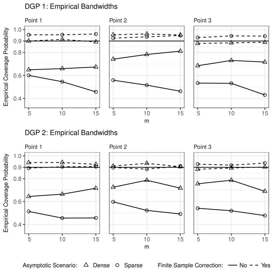
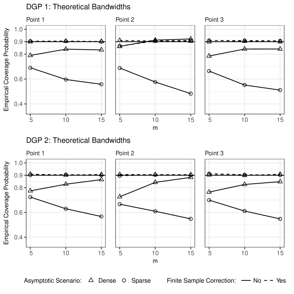
The two top panels in Figure 1 show the empirical coverage probabilities of the feasible confidence intervals with plugged-in estimates $\hat{h}^{S}_{\mu,U}$, $\hat{h}^{S}_{\mu,Z}$, $\hat{h}^{D}_{\mu,U}$, $\hat{h}^{D}_{\mu,Z}$, $\hat{B}_{\mu}$, $\hat{B}^{D}_{\mu}$, $\hat{V}^{I}_{\mu}$, and $\hat{V}^{II}_{\mu}$ from Sections 5.1 and 5.2. The two bottom panels show the empirical coverage probabilities of the infeasible theoretical confidence intervals based on the theoretical bandwidth, bias, and variance expressions. The infeasible confidence intervals serve as validating benchmarks, since they allow us to abstract from the additional estimation errors that are due to the plug-in estimates. We use $(1-\alpha/2)=0.9$ as our nominal coverage probability.

Let us first consider the feasible version of the sparse confidence interval $\operatorname{CI}^{S}$. This is an interesting special case, since essentially the same confidence interval would be used by a practitioner who takes the asymptotic normality result in Theorem 3.2 of Jiang and Wang (2010) as a theoretical basis. This confidence interval shows a very poor performance with far to small coverage probabilities. The problem occurs in our sparse data scenario with sample sizes $m=5$ and $n=100$ and – as expected – becomes worse as $m$ increases.

By contrast, the feasible version of the dense confidence interval $\operatorname{CI}^{D}$ performs quite satisfactorily. Though, the best and most stable results are achieved by the feasible versions of the confidence intervals with finite-sample corrections, $\operatorname{CI}^{S}_{C}$ and $\operatorname{CI}^{D}_{C}$, both showing an almost equally good performance. All of our results on the feasible confidence intervals are essentially equivalent to those for the infeasible theoretical benchmark confidence intervals shown in the two bottom panels in Figure 2. This comparison serves as a validation of our simulation results, since it shows that the results are not driven by bad and too imprecise plug-in estimates.

Table 1: Empirical versus theoretical variances. The figures in the upper panel are based on the sparse bandwidths, $\hat{h}^{S}_{\mu,U}$ and $\hat{h}^{S}_{\mu,Z}$, from Eq.s (16) and (17); those of the lower panel are based on the dense bandwidths, $\hat{h}^{D}_{\mu,U}$ and $\hat{h}^{D}_{\mu,Z}$, from Eq.s (20) and (21).
DGP-1 DGP-2
Point 1: $(u,z)=(0.25,0.75)$ m=5 m=10 m=15 m=5 m=10 m=15
$\widehat{\text{Var}}\big{(}\hat{\mu}(u,z)\big{)}$/ $V^{I}_{\mu}(u,z)$ 2.9 3.3 6.7 3.1 3.5 4.1
$\widehat{\text{Var}}\big{(}\hat{\mu}(u,z)\big{)}$/ $\big{(}V^{I}_{\mu}(u,z)+V^{II}_{\mu}(u,z)\big{)}$ 1.2 1.3 1.5 1.0 0.9 0.9
$\widehat{\text{Var}}\big{(}\hat{\mu}(u,z)\big{)}$/ $V^{II}_{\mu}(u,z)$ 1.7 1.3 1.6 1.8 1.3 1.5
$\widehat{\text{Var}}\big{(}\hat{\mu}(u,z)\big{)}$/ $\big{(}V^{I}_{\mu}(u,z)+V^{II}_{\mu}(u,z)\big{)}$ 0.9 1.1 1.1 1.0 0.9 1.0

The reason for the poor performance of the confidence interval $\operatorname{CI}^{S}$ is shown in the first row of Table 1. The variance term $V_{\mu}^{I}=V^{I}_{\mu}(u,z)$ used to construct $\operatorname{CI}^{S}$, severely underestimates the finite-sample variance $\widehat{\text{Var}}(\hat{\mu})=\widehat{\text{Var}}(\hat{\mu}(u,z))$ of the LLK estimator $\hat{\mu}(u,z)$, where $\widehat{\text{Var}}(\hat{\mu})$ is computed from the 5000 Monte Carlo replications. For $m=5$, the first variance term, $V^{I}_{\mu}$, is $2.9$ and $3.1$ times smaller than the actual finite-sample variance $\widehat{\text{Var}}(\hat{\mu})$ and – as expected – the ratio becomes worse as $m$ increases. This leads to too narrow confidence intervals $\operatorname{CI}^{S}$ and hence to too small coverage probabilities. This observation is in line with the relatively small $\theta=1/5$ threshold for differentiating between sparse and dense functional data. The small $\theta=1/5$ threshold implies that the functional-data-specific second variance term $V_{\mu}^{II}$ will be non-negligible in real data scenarios where $m$ is relatively small in comparison to $n^{1/5}$. Therefore, including the second variance terms $V^{II}_{\mu}(u,z)$ leads to strongly improved approximations of the finite-sample variances of $\hat{\mu}$; see the second and fourth row in Table 1. This explains the superior performances of the confidence intervals, $\operatorname{CI}^{S}_{C}$ and $\operatorname{CI}^{D}_{C}$, incorporating our finite-sample corrections.

For evaluating the estimation results with respect to the covariance function, we consider the average integrated squared error $\int_{0}^{1}\int_{0}^{1}\int_{0}^{1}\big{(}\hat{\gamma}(u_{1},u_{2},z)-\gamma(u_{1},u_{2},z)\big{)}^{2}du_{1}du_{2}dz$ based on 100 Monte Carlo simulations using the sparse and dense rule-of-thumb bandwidth approximations of Section 5. Table 2 shows that the sparse and dense bandwidths perform both comparably well. The performance of the sparse bandwidths gets slightly worse as $m$ increases and the performance of the dense bandwidths slightly improve as $m$ increases.

Table 2: Average integrated squared error $\int_{0}^{1}\int_{0}^{1}\int_{0}^{1}\big{(}\hat{\gamma}(u_{1},u_{2},z)-\gamma(u_{1},u_{2},z)\big{)}^{2}du_{1}du_{2}dz$.
Bandwidths $m=5$ $m=10$ $m=15$
DGP1 Sparse 0.0012 0.0015 0.0020
Dense 0.0015 0.0012 0.0007
DGP2 Sparse 0.0015 0.0016 0.0022
Dense 0.0019 0.0017 0.0012

5 Bandwidth, bias and variance approximations

5.1 Rule-of-thumb bandwidth approximations

Our above bandwidth expressions are infeasible as they depend on the unknown quantities $\mathcal{I}_{\mu,UU}$, $\mathcal{I}_{\mu,UZ}$, $\mathcal{I}_{\mu,ZZ}$, $Q_{\mu,1}$, $Q_{\mu,2}$, $\mathcal{I}_{\gamma,U_{(1)}U_{(1)}}$, $\mathcal{I}_{\gamma,U_{(1)}Z}$, $\mathcal{I}_{\gamma,ZZ}$, $Q_{\gamma,1}$, and $Q_{\gamma,2}$. Following Fan and Gijbels (1996), we suggest approximating them using global polynomial regression models. In the following we list our rule-of-thumb approximations for the bandwidths in Eq.s (7)-(14):
Sparse rule-of-thumb bandwidths for $\hat{\mu}$:

$\displaystyle\hat{h}^{S}_{\mu,U}$ $\displaystyle=\left(\frac{R(K_{\mu})\,Q_{\mu,1}\,\hat{\mathcal{I}}_{\mu_{\text{poly}},ZZ}^{3/4}}{nm\,\left(\nu_{2}(K_{\mu})\right)^{2}\,\left[\hat{\mathcal{I}}_{\mu_{\text{poly}},UU}^{1/2}\,\hat{\mathcal{I}}_{\mu,ZZ}^{1/2}+\hat{\mathcal{I}}_{\mu_{\text{poly}},UZ}\right]\hat{\mathcal{I}}_{\mu_{\text{poly}},UU}^{3/4}}\right)^{1/6}$ (16)
$\displaystyle\hat{h}^{S}_{\mu,Z}$ $\displaystyle=\left(\frac{\hat{\mathcal{I}}_{\mu_{\text{poly}},UU}}{\hat{\mathcal{I}}_{\mu_{\text{poly}},ZZ}}\right)^{1/4}\hat{h}^{S}_{\mu,U}$ (17)

Sparse rule-of-thumb bandwidths for $\hat{\gamma}$:

$\displaystyle\hat{h}^{S}_{\gamma,U}$ $\displaystyle=\left(\frac{R(K_{\gamma})\;\hat{Q}_{\gamma_{\text{poly}},1}\;4\;\sqrt{2}\;\hat{\mathcal{I}}_{\gamma_{\text{poly}},ZZ}^{3/2}}{nM\,\left(\nu_{2}(K_{\gamma})\right)^{2}\,\left(2\,\left(\nu_{2}(K_{\gamma})\right)^{2}\,\hat{\mathcal{I}}_{\gamma_{\text{poly}},U_{(1)}Z}+\hat{C}_{\mathcal{I}}\right)\,\left(\hat{C}_{\mathcal{I}}-\hat{\mathcal{I}}_{\gamma_{\text{poly}},U_{(1)}Z}\right)^{3/2}}\right)^{1/7}$ (18)
$\displaystyle\hat{h}^{S}_{\gamma,Z}$ $\displaystyle=\left(\frac{\hat{C}_{\mathcal{I}}-\hat{\mathcal{I}}_{\gamma_{\text{poly}},U_{(1)}Z}}{2\,\hat{\mathcal{I}}_{\gamma,ZZ}}\right)^{1/2}\hat{h}^{S}_{\gamma,U},\;\text{where}$ (19)
$\displaystyle\hat{C}_{\mathcal{I}}$ $\displaystyle=(\hat{\mathcal{I}}_{\gamma_{\text{poly}},U_{(1)}Z}^{2}+4\,(\hat{\mathcal{I}}_{\gamma_{\text{poly}},U_{(1)}U_{(1)}}+\hat{\mathcal{I}}_{\gamma_{\text{poly}},U_{(1)}U_{(2)}})\,\hat{\mathcal{I}}_{\gamma_{\text{poly}},ZZ})^{1/2}.$

Dense rule-of-thumb bandwidths for $\hat{\mu}$:

$\displaystyle\hat{h}^{D}_{\mu,Z}$ $\displaystyle=\left(\frac{R(\kappa)\,\hat{Q}_{\mu_{\text{poly}},2}}{n\,\left(\nu_{2}(K_{\mu})\right)^{2}\,\hat{\mathcal{I}}_{\mu_{\text{poly}},ZZ}}\right)^{1/5}$ (20)
$\displaystyle\hat{h}^{D}_{\mu,U}$ $\displaystyle=\left(\frac{R(K_{\mu})\,\hat{Q}_{\mu_{\text{poly}},1}}{nm\,\left(\nu_{2}(K_{\mu})\right)^{2}\,\hat{\mathcal{I}}_{\mu_{\text{poly}},UZ}}\right)^{1/3}\left(\hat{h}^{D}_{\mu,Z}\right)^{-1}$ (21)

Dense rule-of-thumb bandwidths for $\hat{\gamma}$:

$\displaystyle\hat{h}^{D}_{\gamma,Z}$ $\displaystyle=\left(\frac{R(\kappa)\,\hat{Q}_{\gamma_{\text{poly}},2}}{n\,\left(\nu_{2}(K_{\gamma})\right)^{2}\,\hat{\mathcal{I}}_{\gamma_{\text{poly}},ZZ}}\right)^{1/5}$ (22)
$\displaystyle\hat{h}^{D}_{\gamma,U}$ $\displaystyle=\left(\frac{R(K_{\gamma})\,\hat{Q}_{\gamma_{\text{poly}},1}}{nM\,\left(\nu_{2}(K_{\gamma})\right)^{2}\,\hat{\mathcal{I}}_{\gamma_{\text{poly}},U_{(1)}Z}}\right)^{1/4}\left(\hat{h}^{D}_{\gamma_{\text{poly}},Z}\right)^{-3/4}$ (23)

The above rule-of-thumb bandwidth expressions are based on the following estimates for the sparse rule-of-thumb bandwidths:

$$\begin{array}[]{rcl}\hat{\mathcal{I}}_{\mu_{\text{poly}},UU}&=&\int_{\operatorname{supp}(f_{UZ})}(\hat{\mu}_{\text{poly}}^{(2,0)}(u,z))^{2}\,\hat{f}_{UZ}(u,z)\,d(u,z),\\[4.30554pt] \hat{\mathcal{I}}_{\mu_{\text{poly}},UZ}&=&\int_{\operatorname{supp}(f_{UZ})}\hat{\mu}_{\text{poly}}^{(2,0)}(u,z)\hat{\mu}_{\text{poly}}^{(0,2)}(u,z)\,\hat{f}_{UZ}(u,z)\,d(u,z),\\[4.30554pt] \hat{\mathcal{I}}_{\mu_{\text{poly}},ZZ}&=&\int_{\operatorname{supp}(f_{UZ})}(\hat{\mu}_{\text{poly}}^{(0,2)}(u,z))^{2}\,\hat{f}_{UZ}(u,z)\,d(u,z),\\[4.30554pt] \hat{Q}_{\mu_{\text{poly}},1}&=&\int_{\operatorname{supp}(f_{UZ})}\hat{\gamma}^{\text{ND}}_{\text{poly}}(u,u,z)\,d(u,z),\\[4.30554pt] \hat{Q}_{\mu_{\text{poly}},2}&=&\int_{\operatorname{supp}(f_{UZ})}\hat{\gamma}_{\text{poly}}(u,u,z)\,\hat{f}_{U}(u)\,d(u,z),\end{array}$$

and for the dense rule-of-thumb bandwidths:

$$\begin{array}[]{rcl}\hat{\mathcal{I}}_{\gamma_{\text{poly}},U_{(1)}U_{(1)}}&=&\int_{\operatorname{supp}(f_{UZ})}(\hat{\gamma}_{\text{poly}}^{(2,0,0)}(u,u,z))^{2}\,\hat{f}_{UZ}(u,z)\,d(u,z),\\[4.30554pt] \hat{\mathcal{I}}_{\gamma_{\text{poly}},U_{(1)}Z}&=&\int_{\operatorname{supp}(f_{UUZ})}\hat{\gamma}_{\text{poly}}^{(2,0,0)}(u,u,z)\hat{\gamma}_{\text{poly}}^{(0,0,2)}(u,u,z)\,\hat{f}_{UUZ}(u,u,z)\,d(u,u,z),\\[4.30554pt] \hat{\mathcal{I}}_{\gamma_{\text{poly}},ZZ}&=&\int_{\operatorname{supp}(f_{UUZ})}(\hat{\gamma}_{\text{poly}}^{(0,0,2)}(u,u,z))^{2}\,\hat{f}_{UUZ}(u,u,z)\,d(u,u,z),\\[4.30554pt] \hat{Q}_{\gamma_{\text{poly}},1}&=&\int_{\operatorname{supp}(f_{UUZ})}\hat{\tilde{\gamma}}^{\text{ND}}_{\text{poly}}((u_{1},u_{2}),(u_{1},u_{2}),z)\,d(u_{1},u_{2},z),\quad\text{and}\\[4.30554pt] \hat{Q}_{\gamma_{\text{poly}},2}&=&\int_{\operatorname{supp}(f_{UUZ})}\hat{\tilde{\gamma}}_{\text{poly}}((u_{1},u_{2}),(u_{1},u_{2}),z)\;\hat{f}_{UU}(u_{1},u_{2})\,d(u_{1},u_{2},z).\end{array}$$

The estimates $\hat{\mu}_{\text{poly}}$, $\hat{\gamma}^{\text{ND}}_{\text{poly}}$, $\hat{\gamma}_{\text{poly}}$, $\hat{\tilde{\gamma}}^{\text{ND}}_{\text{poly}}$, $\hat{\tilde{\gamma}}_{\text{poly}}$, $\hat{\mu}_{\text{poly}}^{(2,0)}$, $\hat{\mu}_{\text{poly}}^{(0,2)}$, $\hat{\gamma}_{\text{poly}}^{(2,0,0)}$, and $\hat{\gamma}_{\text{poly}}^{(0,0,2)}$ are the ordinary least squares estimates (and their derivatives) of the following polynomial regression models:


$\boldsymbol{\mu}_{\textbf{poly}}\textbf{:}$ The model $\mu_{\text{poly}}(u,z)$ is fitted via regressing $Y_{ij}$ on powers (each up to the fourth power) of $U_{ij}$, $Z_{i}$, and $U_{ij}\cdot Z_{i}$ for all $i\in\{1,\dots,n\}$ and $j\in\{1,\dots,m\}$, i.e., $Y_{ij}=\mu_{\text{poly}}(U_{ij},Z_{i})+\text{error}_{ij}$, where $\mu_{\text{poly}}(U_{ij},Z_{i})=\beta_{0}+\sum_{q=1}^{4}\left(\beta^{U}_{q}U_{ij}^{q}+\beta^{Z}_{q}Z_{ij}^{q}+\beta^{UZ}_{q}(U_{ij}Z_{i})^{q}\right).$


$\boldsymbol{\gamma}_{\textbf{poly}}$: The model $\gamma_{\text{poly}}(u_{1},u_{2},z)$ is fitted via regressing $C^{\text{poly}}_{ijk}$ on powers (each up to the fourth power) of $U_{ij}$, $U_{ik}$, $Z_{i}$, $U_{ij}\cdot Z_{i}$, and $U_{ik}\cdot Z_{i}$ for all $i\in\{1,\dots,n\}$ and all $j,k\in\{1,\dots,m\}$ with $j\neq k$, i.e., $C^{\text{poly}}_{ijk}=\gamma_{\text{poly}}(U_{ij},U_{ik},Z_{i})+\text{error}_{ijk}$, where $C^{\text{poly}}_{ijk}=(Y_{ij}-\mu_{\text{poly}}(U_{ij},Z_{i}))(Y_{jt}-\mu_{\text{poly}}(U_{ik},Z_{i}))$ and
$\gamma_{\text{poly}}(U_{ij},U_{ik},Z_{i})=\beta_{0}+\sum_{q=1}^{4}\big{(}\beta^{U,1}_{q}U_{ij}^{q}+\beta^{U,2}_{q}U_{ik}^{q}+\beta^{Z}_{q}Z_{i}^{q}+\beta^{UZ,1}_{q}(U_{ij}Z_{i})^{q}+\beta^{UZ,2}_{q}(U_{ik}Z_{i})^{q}\big{)}.$


$\boldsymbol{\tilde{\gamma}}_{\textbf{poly}}$: The model $\tilde{\gamma}_{\text{poly}}((u_{1},u_{2}),(u_{3},u_{4}),z)$ is fitted via regressing $\mathbb{C}^{\text{poly}}_{ijk\ell m}$ on powers (each up to the fourth power) of $U_{ij}$, $U_{ik}$, $U_{i\ell}$, $U_{im}$, and $Z_{i}$ for all $i\in\{1,\dots,n\}$ and all $j,k,\ell,m\in\{1,\dots,m\}$ such that ($j\neq\ell$ AND $k\neq m$), i.e., $\mathbb{C}^{\text{poly}}_{ijk\ell m}=\tilde{\gamma}_{\text{poly}}((U_{ij},U_{ik}),(U_{i\ell},U_{im}),Z_{i})+\text{error}_{ijk\ell m}$, where $\mathbb{C}^{\text{poly}}_{ijk\ell m}=(C^{\text{poly}}_{ijk}-\gamma_{\text{poly}}(U_{ij},U_{ik},Z_{i}))(C^{\text{poly}}_{i\ell m}-\gamma_{\text{poly}}(U_{i\ell},U_{im},Z_{i}))$ and
$\tilde{\gamma}_{\text{poly}}((U_{ij},U_{ik}),(U_{i\ell},U_{im}),Z_{i})=\beta_{0}+\sum_{q=1}^{4}\left(\beta_{q}^{U,1}U_{ij}^{q}+\beta_{q}^{U,2}U_{ik}^{q}+\beta_{q}^{U,3}U_{i\ell}^{q}+\beta_{q}^{U,4}U_{im}^{q}+\beta_{q}^{Z}Z_{i}^{q}+\right.$ $\left.+\beta_{q}^{UZ,1}(U_{ij}Z_{i})^{q}+\beta_{q}^{UZ,2}(U_{ik}Z_{i})^{q}+\beta_{q}^{UZ,3}(U_{i\ell}Z_{i})^{q}+\beta_{q}^{UZ,4}(U_{im}Z_{i})^{q}\right).$


$\boldsymbol{\gamma}^{\textbf{S}}_{\textbf{poly}}$: The model $\gamma^{\text{ND}}_{\text{poly}}(u,u,z)$ is fitted via regressing the noise-contaminated diagonal values $C^{\text{poly}}_{ij}$ on powers (each up to the fourth power) of $U_{ij}$, and $Z_{i}$ for all $i\in\{1,\dots,n\}$ and $j\in\{1,\dots,m\}$, i.e., $C^{\text{poly}}_{ij}=\gamma^{\text{ND}}_{\text{poly}}(U_{ij},U_{ij},Z_{i})+\text{error}_{ij}$, where $C^{\text{poly}}_{ij}=(Y_{ij}-\mu_{\text{poly}}(U_{ij},Z_{i}))^{2}$ and $\gamma^{\text{ND}}_{\text{poly}}(U_{ij},U_{ij},Z_{i})=\beta_{0}+\sum_{q=1}^{4}\left(\beta^{U}_{q}U_{ij}^{q}+\beta^{Z}_{q}Z_{i}^{q}+\beta^{UZ}_{q}(U_{ij}Z_{i})^{q}\right).$ The ND in $\gamma^{\text{ND}}_{\text{poly}}$ suggest that we are estimating the noise-contaminated diagonal values $\gamma(u,u,z)+\sigma_{\epsilon}$.


$\boldsymbol{\tilde{\gamma}}^{\textbf{S}}_{\textbf{poly}}$: The model $\tilde{\gamma}^{\text{ND}}_{\text{poly}}(u_{1},u_{2},z)$ is fitted via regressing the noise-contaminated diagonal values $\mathbb{C}_{ijk}^{\text{poly}}$ on powers (each up to the fourth power) of $U_{ij}$, $U_{ik}$, and $Z_{i}$ for all $i\in\{1,\dots,n\}$, and $j,k\in\{1,\dots,m\}$, i.e., $\mathbb{C}^{\text{poly}}_{ijk}=\tilde{\gamma}^{\text{ND}}_{\text{poly}}(U_{ij},U_{ik},Z_{i})+\text{error}_{ijk}$, where $\mathbb{C}^{\text{poly}}_{ijk}=(C^{\text{poly}}_{ijk}-\gamma_{\text{poly}}(U_{ij},U_{ik},Z_{i}))^{2}$ and $\tilde{\gamma}^{\text{ND}}_{\text{poly}}(U_{ij},U_{ik},Z_{i})=\beta_{0}+\sum_{q=1}^{4}\left(\beta_{q}^{U,1}U_{ij}^{q}+\beta_{q}^{U,2}U_{ik}^{q}+\beta_{q}^{Z}Z_{i}^{q}\right).$ The ND in $\tilde{\gamma}^{\text{ND}}_{\text{poly}}$ suggest that we are estimating the noise-contaminated diagonal values $\tilde{\gamma}((u_{1},u_{2}),(u_{1},u_{2}),z)+\sigma_{\varepsilon}(u_{1},u_{2},z)$.

Estimates of the densities $f_{UZ}$ and $f_{UUZ}$ are computed as kernel density estimates using Gaussian kernels and bandwidth determined by cross-validation.

Remark

It is important to specify the models $\boldsymbol{\mu_{\text{poly}}}$ and $\boldsymbol{\gamma_{\text{poly}}}$ using interaction terms, since otherwise their partial derivatives $\hat{\mu}_{\text{poly}}^{(2,0)}$, $\hat{\mu}_{\text{poly}}^{(0,2)}$, $\hat{\gamma}_{\text{poly}}^{(2,0,0)}$, and $\hat{\gamma}_{\text{poly}}^{(0,0,2)}$ would degenerate.

5.2 Bias and variance estimates

Following Härdle and Bowman (1988), we approximate the unknown second derivatives $\mu^{(2,0)}$ and $\mu^{(0,2)}$ in $B_{\mu}$ and $B^{D}_{\mu}$ using local polynomial estimators. That is, we approximate $B_{\mu}(u,z;h_{\mu,U},h_{\mu,Z})$ and $B^{D}_{\mu}(u,z;h_{\mu,Z})$ by

$$\begin{array}[]{rcl}\hat{B}_{\mu}(u,z;h_{\mu,U},h_{\mu,Z})&=&\frac{\nu_{2}(K_{\mu})}{2}\Big{(}h_{\mu,U}^{2}\hat{\mu}^{(2,0)}\big{(}u,z;g_{\mu,U},g_{\mu,Z}\big{)}+h_{\mu,Z}^{2}\hat{\mu}^{(0,2)}\big{(}u,z;g_{\mu,U},g_{\mu,Z}\big{)}\Big{)}\\[8.61108pt] \text{and}\quad\hat{B}^{D}_{\mu}(u,z;h_{\mu,Z})&=&\frac{\nu_{2}(K_{\mu})}{2}h_{\mu,Z}^{2}\hat{\mu}^{(0,2)}\big{(}u,z;g_{\mu,U},g_{\mu,Z}\big{)}\end{array}$$

where $\hat{\mu}^{(2,0)}$ and $\hat{\mu}^{(0,2)}$ are local polynomial (order $3$) kernel estimators of $\mu^{(2,0)}$ and $\mu^{(0,2)}$:

$$\begin{array}[]{l}\hat{\mu}^{(2,0)}(u,z;g_{\mu,U},g_{\mu,Z})=2!\,e_{3}^{\top}\left([\mathbf{1},\mathbf{U}_{u}^{1:3},\mathbf{Z}_{z}^{1:3}]^{\top}\mathbf{W}_{\mu,uz}[\mathbf{1},\mathbf{U}_{u}^{1:3},\mathbf{Z}_{z}^{1:3}]\right)^{-1}[\mathbf{1},\mathbf{U}_{u}^{1:3},\mathbf{Z}_{z}^{1:3}]^{\top}\mathbf{W}_{\mu,uz}\mathbf{Y}\\ \hat{\mu}^{(0,2)}(u,z;g_{\mu,U},g_{\mu,Z})=2!\,e_{6}^{\top}\left([\mathbf{1},\mathbf{U}_{u}^{1:3},\mathbf{Z}_{z}^{1:3}]^{\top}\mathbf{W}_{\mu,uz}[\mathbf{1},\mathbf{U}_{u}^{1:3},\mathbf{Z}_{z}^{1:3}]\right)^{-1}[\mathbf{1},\mathbf{U}_{u}^{1:3},\mathbf{Z}_{z}^{1:3}]^{\top}\mathbf{W}_{\mu,uz}\mathbf{Y},\end{array}$$

with $e_{3}^{\top}=(0,0,1,0,0,0,0)$, $e_{6}^{\top}=(0,0,0,0,0,1,0)$, $\mathbf{U}_{u}^{1:3}=[\mathbf{U}_{u},\mathbf{U}_{u}^{2},\mathbf{U}_{u}^{3}]$, $\mathbf{Z}_{z}^{1:3}=[\mathbf{Z}_{z},\mathbf{Z}_{z}^{2},\mathbf{Z}_{z}^{3}]$, and $\mathbf{W}_{\mu,uz}=\operatorname{diag}(\dots,g^{-1}_{\mu,U}\,\kappa(g^{-1}_{\mu,U}(U_{ij}-u))\;g^{-1}_{\mu,Z}\,\kappa(g^{-1}_{\mu,Z}(Z_{i}-z)),\dots)$.

For estimating the bandwidths $g_{\mu,U}$ and $g_{\mu,Z}$ we use bivariate GCV based on second-order differences. We follow the procedure of Charnigo and Srinivasan (2015), but use a GCV-penalty instead of their proposed (asymptotically equivalent) $C_{p}$-penalty.

For approximating the unknown noise-contaminated diagonal of the covariance function, $\gamma(u,u,z)+\sigma_{\epsilon}^{2}$, contained in $V_{\mu}^{I}$, we propose to use a LLK estimator. That is, we approximate $V_{\mu}^{I}$ by

$\displaystyle\hat{V}_{\mu}^{I}(u,z;h_{\mu,U},h_{\mu,Z},h_{\gamma,U},h_{\gamma,Z})$ $\displaystyle=(nm)^{-1}\left[(h_{\mu,U}h_{\mu,Z})^{-1}R(K_{\mu})\frac{\hat{\gamma}^{\text{ND}}(u,u,z;h_{\gamma,U},h_{\gamma,Z})}{\hat{f}_{UZ}(u,z)}\,\right]$

where the estimator of the Noisy Diagonal (ND), $\hat{\gamma}^{\text{ND}}(u,u,z;h_{\gamma,U},h_{\gamma,Z})\approx\{\gamma(u,u,z)+\sigma_{\epsilon}^{2}\}$, is defined as the following LLK estimator:

$\displaystyle\hat{\gamma}^{\text{ND}}(u,u,z;h_{\gamma,U},h_{\gamma,Z})=e_{1}^{\top}\left([\mathbf{1},\mathbf{U}_{u},\mathbf{Z}_{z}]^{\top}\mathbf{W}_{\gamma,uz}[\mathbf{1},\mathbf{U}_{u},\mathbf{Z}_{z}]\right)^{-1}[\mathbf{1},\mathbf{U}_{u},\mathbf{Z}_{z}]^{\top}\mathbf{W}_{\gamma,uz}\hat{\mathbf{C}},$

where $\hat{\mathbf{C}}=(\hat{C}_{111},\dots,C_{ijj}\dots,\hat{C}_{nmm})^{\top}$ consists only of the diagonal raw-covariances, i.e., $\hat{C}_{ijj}=(Y_{ij}-\hat{\mu}(U_{ij},Z_{i};h_{\mu,U},h_{\mu,Z}))^{2}$. Note that $\hat{\gamma}^{\text{ND}}$ is equivalent to the LLK estimator $\hat{V}$ in Jiang and Wang (2010).

Finally, for estimating the unknown quantity $\gamma(u,u,z)$ in $V_{\mu}^{II}$ we can use our LLK estimator $\hat{\gamma}(u,u,z;h_{\gamma,U},h_{\gamma,Z})$ as defined in (6). That is we estimate $V_{\mu}^{II}$ by

$\displaystyle\hat{V}_{\mu}^{II}(u,z;h_{\mu,Z},h_{\gamma,U},h_{\gamma,Z})$ $\displaystyle=n^{-1}\left[\left(\frac{m-1}{m}\right)(h_{\mu,Z})^{-1}\,R(\kappa)\frac{\hat{\gamma}(u,u,z;h_{\gamma,U},h_{\gamma,Z})}{\hat{f}_{Z}(z)}\right].$

The bandwidths for the LLK estimators $\hat{\gamma}$ and $\hat{\gamma}^{\text{ND}}$ are selected according to our Rule-of-thumb bandwidth approximations in Eq.s (18), (19), (22), and (23). An alternative approach to the above proposed rule-of-thumb approximations might be to completely adapt the bootstrap procedure of Härdle and Bowman (1988), which is, however, computationally more demanding.

6 Application

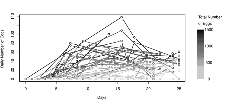
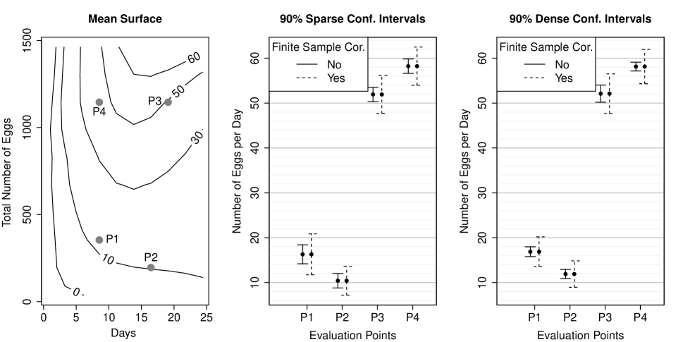
We consider the well-known reproductive data for Mediterranean fruit flies (Ceratitis capitata) as provided in the R-package fdapace of Dai et al. (2017). This is a subsample of the data previously analyzed in Carey et al. (1998) containing the daily numbers of eggs laid from 789 medflies during the first 25 days of their lives. As Jiang and Wang (2010), we construct a sparse data set by randomly selecting without replacement $m=10$ observations from the 25 measurements of each fruit fly. Random selections of $m=5$ or $m=15$ observations lead to qualitatively equivalent results. Following the original analysis in Carey et al. (1998), we analyze the relationship between the daily reproduction $Y_{ij}$, measured at day $U_{ij}$, and the total reproduction $Z_{i}$. Figure 3 shows the data, where we only display a subset of 50 randomly selected trajectories to prevent an overcrowded and unclear plot. The left panel in Figure 4 shows the contour plot of the surface of the estimated mean function using our sparse bandwidths and essentially replicates Figure 7 of the original analysis in Carey et al. (1998). The contour lines clearly indicate a dependency between the daily mean reproduction and the total mean reproduction of medflies.

Refer to caption
Figure 3: Mediterranean fruit flies data originally analyzed by Carey et al. (1998).

In order to showcase the relevance of our theoretical results, we select four points, P1, P2, P3, and P4, and compare their confidence intervals based on the sparse ($\operatorname{CI}^{S}_{C}$ and $\operatorname{CI}^{S}$) and dense ($\operatorname{CI}^{D}_{C}$ and $\operatorname{CI}^{D}$) asymptotic scenarios with and without finite sample correction (see middle and right panel of Figure 4). A Bonferroni correction is used to adjust for the multiple testing. From our simulation study we know that the variance components of the confidence intervals without finite sample corrections tend to underestimate the actual variance of the nonparametric mean estimator. That is, inference based on the confidence intervals without finite sample corrections will have a tendency for over-rejection of the null-hypotheses of equal means, due to an under-estimated pointwise variance component in finite samples.

This adverse effect can be seen when using the confidence intervals in order to check for significant differences between P1 vs. P2 and P3 vs. P4. The confidence intervals without finite sample corrections ($\operatorname{CI}^{S}$ and $\operatorname{CI}^{D}$) are extremely narrow and suggest significant differences between the means at P1 vs. P2 and P3 vs. P4. These significant differences are quite implausible, since the points P1 and P2 as well as P3 and P4 lie almost at the same contour lines. By contrast, the confidence intervals with our finite sample corrections ($\operatorname{CI}_{C}^{S}$ and $\operatorname{CI}_{C}^{D}$) are considerably wider and do not indicate such implausibly significant differences. Qualitatively similar results can be showcased, e.g., for $m=5$ and $m=15$; however, their display is omitted in order not to unnecessarily prolong the manuscript.

Refer to caption
Figure 4: Left Panel: Contour plot of the estimated mean function. Middle and Right Panel: 90% sparse and dense confidence intervals without finite sample correction (solid lines) and with finite sample correction (dashed line).

Acknowledgements

I want to thank Alois Kneip (University of Bonn) and Piotr Kokoszka (Colorado State University) for fruitful discussions and valuable comments which helped to improve this research work. Additionally, I want to thank Irène Gijbels (KU Leuven) and Jane-Ling Wang (UC Davis) for valuable comments on my talk at the CMStatistics in 2015 where I presented an earlier version of this manuscript. Many thanks go to the student assistants of the Institute of Financial Economics and Statistics of the University of Bonn for coding assistance.

Appendix A Proofs

A.1 Proof of Theorem 3.1

Proof of Theorem 3.1, part (i): For simplicity, consider a second-order kernel function $\kappa$ with compact support such as the Epanechnikov kernel. This is, of course, without loss of generality, but allows for a more compact proof. Define $\mathbf{H}_{\mu}=\operatorname{diag}(h^{2}_{\mu,U},h^{2}_{\mu,Z})$, $\mathbf{U}=(U_{11},\dots,U_{nm})^{\top}$, and $\mathbf{Z}=(Z_{1},\dots,Z_{n})^{\top}$. Using a Taylor-expansion of $\mu$ around $(u,z)$, the conditional bias of the estimator $\hat{\mu}(u,z;\mathbf{H})$ can be written as

$\displaystyle\operatorname{\mathbb{E}}(\hat{\mu}(u,z;\mathbf{H}_{\mu})-\mu(u,z)|\mathbf{U},\mathbf{Z})=\frac{1}{2}e_{1}^{\top}\left((nm)^{-1}[\mathbf{1},\mathbf{U}_{u},\mathbf{Z}_{z}]^{\top}\mathbf{W}_{\mu,uz}[\mathbf{1},\mathbf{U}_{u},\mathbf{Z}_{z}]\right)^{-1}\times$ (24)
$\displaystyle\times(nm)^{-1}[\mathbf{1},\mathbf{U}_{u},\mathbf{Z}_{z}]^{\top}\mathbf{W}_{\mu,uz}\left(\boldsymbol{\mathcal{Q}}_{\mu}(u,z)+\mathbf{R}_{\mu}(u,z)\right),$

where $\boldsymbol{\mathcal{Q}}_{\mu}(u,z)$ is a $nm\times 1$ vector with typical elements

$\displaystyle(U_{ij}-u,Z_{i}-z)\boldsymbol{\mathcal{H}}_{\mu}(u,z)(U_{ij}-u,Z_{i}-z)^{\top}\in\mathbb{R}$

with $\boldsymbol{\mathcal{H}}_{\mu}(u,z)$ being the Hessian matrix of the regression function $\mu(u,z)$. The $nm\times 1$ vector $\mathbf{R}_{\mu}(u,z)$ holds the remainder terms as in Ruppert and Wand (1994).

Next we derive asymptotic approximations for the $3\times 3$ matrix
$\left((nm)^{-1}[\mathbf{1},\mathbf{U}_{u},\mathbf{Z}_{z}]^{\top}\mathbf{W}_{\mu,uz}[\mathbf{1},\mathbf{U}_{u},\mathbf{Z}_{z}]\right)^{-1}$ and the $3\times 1$ matrix $(nm)^{-1}[\mathbf{1},\mathbf{U}_{u},\mathbf{Z}_{z}]^{\top}\mathbf{W}_{\mu,uz}\boldsymbol{\mathcal{Q}}_{\mu}(u,z)$ of the right hand side of Eq. (24). Using standard procedures from kernel density estimation it is easy to derive that
$(nm)^{-1}[\mathbf{1},\mathbf{U}_{u},\mathbf{Z}_{z}]^{\top}\mathbf{W}_{\mu,uz}[\mathbf{1},\mathbf{U}_{u},\mathbf{Z}_{z}]=$

$\displaystyle\left(\begin{matrix}f_{UZ}(u,z)+o_{p}(1)&\quad\nu_{2}(K_{\mu})\mathbf{D}_{f_{UZ}}(u,z)^{\top}\mathbf{H}_{\mu}+o_{p}(\mathbf{1}^{\top}\mathbf{H}_{\mu})\\ \nu_{2}(K_{\mu})\mathbf{H}_{\mu}\mathbf{D}_{f_{UZ}}(u,z)+o_{p}(\mathbf{H}_{\mu}\mathbf{1})&\quad\nu_{2}(K_{\mu})\mathbf{H}_{\mu}f_{UZ}(u,z)+o_{p}(\mathbf{H}_{\mu})\\ \end{matrix}\right),$

where $\mathbf{1}=(1,1)^{\top}$ and $\mathbf{D}_{f_{UZ}}(u,z)$ is the vector of first order partial derivatives (i.e., the gradient) of the pdf $f_{UZ}$ at $(u,z)$. Inversion of the above block matrix yields

$\displaystyle\left((nm)^{-1}[\mathbf{1},\mathbf{U}_{u},\mathbf{Z}_{z}]^{\top}\mathbf{W}_{\mu,uz}[\mathbf{1},\mathbf{U}_{u},\mathbf{Z}_{z}]\right)^{-1}=$ (25)
$\displaystyle\left(\begin{matrix}\left(f_{UZ}(u,z)\right)^{-1}+o_{p}(1)&\quad-\mathbf{D}_{f_{UZ}}(u,z)^{\top}\left(f_{UZ}(u,z)\right)^{-2}+o_{p}(\mathbf{1}^{\top})\\ -\mathbf{D}_{f_{UZ}}(u,z)\left(f_{UZ}(u,z)\right)^{-2}+o_{p}(\mathbf{1})&\quad\left(\nu_{2}(K_{\mu})\mathbf{H}_{\mu}f_{UZ}(u,z)\right)^{-1}+o_{p}(\mathbf{H}_{\mu})\\ \end{matrix}\right).$

The $3\times 1$ matrix $(nm)^{-1}[\mathbf{1},\mathbf{U}_{u},\mathbf{Z}_{z}]^{\top}\mathbf{W}_{\mu,uz}\boldsymbol{\mathcal{Q}}_{\mu}(u,z)$ can be partitioned as following:

$\displaystyle(nm)^{-1}[\mathbf{1},\mathbf{U}_{u},\mathbf{Z}_{z}]^{\top}\mathbf{W}_{\mu,uz}\boldsymbol{\mathcal{Q}}_{\mu}(u,z)$ $\displaystyle=$ $\displaystyle\left(\begin{matrix}\texttt{upper element}\\ \texttt{lower bloc}\end{matrix}\right),$

where the $1\times 1$ dimensional upper element can be approximated by

$\displaystyle(nm)^{-1}\sum_{ij}K_{\mu,h}(U_{ij}-u,Z_{i}-z)(U_{ij}-u,Z_{i}-z)\boldsymbol{\mathcal{H}}_{\mu}(u,z)(U_{ij}-u,Z_{i}-z)^{\top}$ (26)
$\displaystyle=$ $\displaystyle\left(\nu_{2}(\kappa)\right)^{2}tr\left\{\mathbf{H}_{\mu}\boldsymbol{\mathcal{H}}_{\mu}(u,z)\right\}f_{UZ}(u,z)+o_{p}(tr(\mathbf{H}_{\mu}))$

and the $2\times 1$ dimensional lower bloc is equal to

$\displaystyle(nm)^{-1}\sum_{ij}\left\{K_{\mu,h}(U_{ij}-u,Z_{i}-z)(U_{ij}-u,Z_{i}-z)\boldsymbol{\mathcal{H}}_{\mu}(u,z)(U_{ij}-u,Z_{i}-z)^{\top}\right\}\times$ (27)
$\displaystyle\times(U_{ij}-u,Z_{i}-z)^{\top}=O_{p}(\mathbf{H}_{\mu}^{3/2}\mathbf{1}).$

Plugging the approximations of Eqs. (25)-(27) into the first summand of the conditional bias expression in Eq. (24) leads to the following expression

$\displaystyle\frac{1}{2}e_{1}^{\top}((nm)^{-1}[\mathbf{1},\mathbf{U}_{u},\mathbf{Z}_{z}]^{\top}\mathbf{W}_{\mu,uz}[\mathbf{1},\mathbf{U}_{u},\mathbf{Z}_{z}])^{-1}(nm)^{-1}[\mathbf{1},\mathbf{U}_{u},\mathbf{Z}_{z}]^{\top}\mathbf{W}_{\mu,uz}\boldsymbol{\mathcal{Q}}_{\mu}(u,z)=$
$\displaystyle=\frac{1}{2}\left(\nu_{2}(\kappa)\right)^{2}tr\left\{\mathbf{H}_{\mu}\boldsymbol{\mathcal{H}}_{\mu}(u,z)\right\}+o_{p}(tr(\mathbf{H}_{\mu})).$

Furthermore, it is easily seen that the second summand of the conditional bias expression in Eq. (24), which holds the remainder term, is given by

$\displaystyle\frac{1}{2}e_{1}^{\top}((nm)^{-1}[\mathbf{1},\mathbf{U}_{u},\mathbf{Z}_{z}]^{\top}\mathbf{W}_{\mu,uz}[\mathbf{1},\mathbf{U}_{u},\mathbf{Z}_{z}])^{-1}(nm)^{-1}[\mathbf{1},\mathbf{U}_{u},\mathbf{Z}_{z}]^{\top}\mathbf{W}_{\mu,uz}\mathbf{R}_{\mu}(u,z)=o_{p}(tr(\mathbf{H}_{\mu})).$

Summation of the two latter expressions yields the asymptotic approximation of the conditional bias

$\displaystyle\operatorname{\mathbb{E}}(\hat{\mu}(u,z;\mathbf{H}_{\mu})-\mu(u,z)|\mathbf{U},\mathbf{Z})=\frac{1}{2}\left(\nu_{2}(\kappa)\right)^{2}tr\left\{\mathbf{H}_{\mu}\boldsymbol{\mathcal{H}}_{\mu}(u,z)\right\}+o_{p}(tr(\mathbf{H}_{\mu})).$

This is our bias statement of Theorem 3.1 part (i).


Proof of Theorem 3.1, part (ii): In the following we derive the conditional variance of the local linear estimator $\operatorname{\mathbb{V}}(\hat{\mu}(u,z;\mathbf{H}_{\mu})|\mathbf{U},\mathbf{Z})=$

$\displaystyle=$ $\displaystyle e_{1}^{\top}([\mathbf{1},\mathbf{U}_{u},\mathbf{Z}_{z}]^{\top}\mathbf{W}_{\mu,uz}[\mathbf{1},\mathbf{U}_{u},\mathbf{Z}_{z}])^{-1}\,[\mathbf{1},\mathbf{U}_{u},\mathbf{Z}_{z}]^{\top}\mathbf{W}_{\mu,uz}\,\mathrm{Cov}(\mathbf{Y}|\mathbf{U},\mathbf{Z})\,\mathbf{W}_{\mu,uz}[\mathbf{1},\mathbf{U}_{u},\mathbf{Z}_{z}]\times$
$\displaystyle\times([\mathbf{1},\mathbf{U}_{u},\mathbf{Z}_{z}]^{\top}\mathbf{W}_{\mu,uz}[\mathbf{1},\mathbf{U}_{u},\mathbf{Z}_{z}])^{-1}u_{1}$
$\displaystyle=$ $\displaystyle e_{1}^{\top}((nm)^{-1}[\mathbf{1},\mathbf{U}_{u},\mathbf{Z}_{z}]^{\top}\mathbf{W}_{\mu,uz}[\mathbf{1},\mathbf{U}_{u},\mathbf{Z}_{z}])^{-1}\times\,$
$\displaystyle\times((nm)^{-2}[\mathbf{1},\mathbf{U}_{u},\mathbf{Z}_{z}]^{\top}\mathbf{W}_{\mu,uz}\,\mathrm{Cov}(\mathbf{Y}|\mathbf{U},\mathbf{Z})\,\mathbf{W}_{\mu,uz}[\mathbf{1},\mathbf{U}_{u},\mathbf{Z}_{z}])\times$
$\displaystyle\times((nm)^{-1}[\mathbf{1},\mathbf{U}_{u},\mathbf{Z}_{z}]^{\top}\mathbf{W}_{\mu,uz}[\mathbf{1},\mathbf{U}_{u},\mathbf{Z}_{z}])^{-1}u_{1},$

where $\mathrm{Cov}(\mathbf{Y}|\mathbf{U},\mathbf{Z})$ is the $nm\times nm$ matrix with typical elements

$\displaystyle\mathrm{Cov}(Y_{ij},Y_{\ell k}|U_{ij},U_{\ell k},Z_{i},Z_{\ell})=\gamma_{|i-\ell|}((U_{ij},Z_{i}),(U_{\ell k},Z_{\ell}))+\sigma_{\epsilon}^{2}\mathbbm{1}{\left(i=\ell\text{ and }j=k\right)}$

with $\mathbbm{1}(.)$ being the indicator function.

We begin with analyzing the $3\times 3$ matrix

$\displaystyle(nm)^{-2}[\mathbf{1},\mathbf{U}_{u},\mathbf{Z}_{z}]^{\top}\mathbf{W}_{\mu,uz}\,\mathrm{Cov}(\mathbf{Y}|\mathbf{U},\mathbf{Z})\,\mathbf{W}_{\mu,uz}[\mathbf{1},\mathbf{U}_{u},\mathbf{Z}_{z}]$

using the following three Lemmas A.1-A.3.

Lemma A.1

The upper-left scalar (block) of the matrix
$(nm)^{-2}[\mathbf{1},\mathbf{U}_{u},\mathbf{Z}_{z}]^{\top}\mathbf{W}_{\mu,uz}\mathrm{Cov}(\mathbf{Y}|\mathbf{U},\mathbf{Z})\mathbf{W}_{\mu,uz}[\mathbf{1},\mathbf{U}_{u},\mathbf{Z}_{z}]$ is given by

$\displaystyle(nm)^{-2}\mathbf{1}^{\top}\mathbf{W}_{\mu,uz}\mathrm{Cov}(\mathbf{Y}|\mathbf{U},\mathbf{Z})\mathbf{W}_{\mu,uz}\mathbf{1}$
$\displaystyle=$ $\displaystyle(nm)^{-1}f_{UZ}(u,z)|\mathbf{H}_{\mu}|^{-1/2}R(K_{\mu})\left(\gamma(u,u,z)+\sigma^{2}_{\epsilon}\right)(1+O_{p}(tr(\mathbf{H}_{\mu}^{1/2})))$
$\displaystyle+$ $\displaystyle n^{-1}(f_{UZ}(u,z))^{2}\left[\left(\frac{m-1}{m}\right)h_{\mu,Z}^{-1}R(\kappa)\frac{\gamma(u,u,z)}{f_{Z}(z)}\right](1+O_{p}(tr(H^{1/2})))$
$\displaystyle=$ $\displaystyle O_{p}((nm)^{-1}|\mathbf{H}_{\mu}|^{-1/2})+O_{p}(n^{-1}h_{\mu,Z}^{-1}).$
Lemma A.2

The $1\times 2$ dimensional upper-right block of the matrix
$(nm)^{-2}[\mathbf{1},\mathbf{U}_{u},\mathbf{Z}_{z}]^{\top}\mathbf{W}_{\mu,uz}\mathrm{Cov}(\mathbf{Y}|\mathbf{U},\mathbf{Z})\mathbf{W}_{\mu,uz}[\mathbf{1},\mathbf{U}_{u},\mathbf{Z}_{z}]$ is given by

$\displaystyle(nm)^{-2}\mathbf{1}^{\top}\mathbf{W}_{\mu,uz}\mathrm{Cov}(\mathbf{Y}|\mathbf{U},\mathbf{Z})\mathbf{W}_{\mu,uz}\left(\begin{matrix}(U_{11}-u,Z_{1}-z)\\ \vdots\\ (U_{nm}-u,Z_{n}-z)\end{matrix}\right)$
$\displaystyle=$ $\displaystyle(nm)^{-1}f_{UZ}(u,z)|\mathbf{H}_{\mu}|^{-1/2}(\mathbf{1}^{\top}\mathbf{H}_{\mu}^{1/2})R(K_{\mu})\left(\gamma(u,u,z)+\sigma^{2}_{\epsilon}\right)(1+O_{p}(tr(\mathbf{H}_{\mu}^{1/2})))$
$\displaystyle+$ $\displaystyle n^{-1}(f_{UZ}(u,z))^{2}(\mathbf{1}^{\top}\mathbf{H}_{\mu}^{1/2})\left[\left(\frac{m-1}{m}\right)h_{\mu,Z}^{-1}R(\kappa)\frac{\gamma(u,u,z)}{f_{Z}(z)}\right](1+O_{p}(tr(\mathbf{H}_{\mu}^{1/2})))$
$\displaystyle=$ $\displaystyle O_{p}((nm)^{-1}|\mathbf{H}_{\mu}|^{-1/2}(\mathbf{1}^{\top}\mathbf{H}_{\mu}^{1/2}))+O_{p}(n^{-1}(\mathbf{1}^{\top}\mathbf{H}_{\mu}^{1/2})h_{\mu,Z}^{-1}).$

The $2\times 1$ dimensional lower-left block of the matrix
$(nm)^{-2}[\mathbf{1},\mathbf{U}_{u},\mathbf{Z}_{z}]^{\top}\mathbf{W}_{\mu,uz}\mathrm{Cov}(\mathbf{Y}|\mathbf{U},\mathbf{Z})\mathbf{W}_{\mu,uz}[\mathbf{1},\mathbf{U}_{u},\mathbf{Z}_{z}]$
is simply the transposed version of this result.

Lemma A.3

The $2\times 2$ lower-right block of the matrix
$(nm)^{-2}[\mathbf{1},\mathbf{U}_{u},\mathbf{Z}_{z}]^{\top}\mathbf{W}_{\mu,uz}\mathrm{Cov}(\mathbf{Y}|\mathbf{U},\mathbf{Z})\mathbf{W}_{\mu,uz}[\mathbf{1},\mathbf{U}_{u},\mathbf{Z}_{z}]$ is given by

$\displaystyle(nm)^{-2}\left(((U_{11}-u),(Z_{1}-z))^{\top},\dots,((U_{nm}-u),(Z_{n}-z)^{\top})\right)\times$
$\displaystyle\times\mathbf{W}_{\mu,uz}\mathrm{Cov}(\mathbf{Y}|\mathbf{U},\mathbf{Z})\mathbf{W}_{\mu,uz}\left(\begin{matrix}(U_{11}-u,Z_{1}-z)\\ \vdots\\ (U_{nm}-u,Z_{n}-z)\end{matrix}\right)$
$\displaystyle=$ $\displaystyle(nm)^{-1}f_{UZ}(u,z)|\mathbf{H}_{\mu}|^{-1/2}\mathbf{H}_{\mu}R(K_{\mu})\left(\gamma(u,u,z)+\sigma^{2}_{\epsilon}\right)(1+O_{p}(tr(\mathbf{H}_{\mu}^{1/2})))$
$\displaystyle+$ $\displaystyle n^{-1}(f_{UZ}(u,z))^{2}\mathbf{H}_{\mu}\left[\left(\frac{m-1}{m}\right)h_{\mu,Z}^{-1}R(\kappa)\frac{\gamma(u,u,z)}{f_{Z}(z)}\right](1+O_{p}(tr(\mathbf{H}_{\mu}^{1/2})))$
$\displaystyle=$ $\displaystyle O_{p}((nm)^{-1}|\mathbf{H}_{\mu}|^{-1/2}\mathbf{H}_{\mu})+O_{p}(n^{-1}\mathbf{H}_{\mu}h_{\mu,Z}^{-1}).$

Using the approximations for the bloc-elements of the matrix
$(nm)^{-2}[\mathbf{1},\mathbf{U}_{u},\mathbf{Z}_{z}]^{\top}\mathbf{W}_{\mu,uz}\mathrm{Cov}(\mathbf{Y}|\mathbf{U},\mathbf{Z})\mathbf{W}_{\mu,uz}[\mathbf{1},\mathbf{U}_{u},\mathbf{Z}_{z}]$, given by the Lemmas A.1-A.3, and the approximation for the matrix $\left((nm)^{-1}[\mathbf{1},\mathbf{U}_{u},\mathbf{Z}_{z}]^{\top}\mathbf{W}_{\mu,uz}[\mathbf{1},\mathbf{U}_{u},\mathbf{Z}_{z}]\right)^{-1}$, given in (25), we can approximate the conditional variance of the bivariate local linear estimator, given in (LABEL:Varexpr). Some tedious yet straightforward matrix algebra leads to $\operatorname{\mathbb{V}}(\hat{\mu}(u,z;\mathbf{H}_{\mu})|\mathbf{U},\mathbf{Z})=$

$\displaystyle(nm)^{-1}|\mathbf{H}_{\mu}|^{-1/2}\left\{\frac{R(K_{\mu})\left(\gamma(u,u,z)+\sigma^{2}_{\epsilon}\right)}{f_{UZ}(u,z)}\right\}\left(1+o_{p}(1)\right)$
$\displaystyle+n^{-1}\left[\left(\frac{m-1}{m}\right)h_{\mu,Z}^{-1}R(\kappa)\frac{\gamma(u,u,z)}{f_{Z}(z)}\right]\left(1+o_{p}(1)\right),$

which is asymptotically equivalent to our variance statement of Theorem 3.1 part (ii).

Next we prove Lemma A.1; the proofs of Lemmas A.2 and A.3 are equivalent. To show Lemma A.1 it will be convenient to split the sum such that
$(nm)^{-2}\mathbf{1}^{\top}\mathbf{W}_{\mu,uz}\mathrm{Cov}(\mathbf{Y}|\mathbf{U},\mathbf{Z})\mathbf{W}_{\mu,uz}\mathbf{1}=s_{1}+s_{2}$. Using standard procedures from kernel density estimation leads to

$\displaystyle s_{1}$ $\displaystyle=(nm)^{-2}\sum_{ij}(K_{\mu,h}(U_{ij}-u,Z_{i}-z))^{2}\operatorname{\mathbb{V}}(Y_{ij}|\mathbf{U},\mathbf{Z})$ (29)
$\displaystyle=(nm)^{-1}|\mathbf{H}_{\mu}|^{-1/2}f_{UZ}(u,z)R(K_{\mu})\left(\gamma(u,u,z)+\sigma^{2}_{\epsilon}\right)+O((nm)^{-1}|\mathbf{H}_{\mu}|^{-1/2}\;tr(\mathbf{H}_{\mu}^{1/2})),$
$\displaystyle s_{2}$ $\displaystyle=(nm)^{-2}\underset{j\neq k}{\sum_{jk}}\sum_{i}h_{\mu,U}^{-1}\kappa(h_{\mu,U}^{-1}(U_{ij}-u))(h_{\mu,Z}^{-1}\kappa(h_{\mu,Z}^{-1}(Z_{i}-z)))^{2}\,\mathrm{Cov}(Y_{ij},Y_{ik}|\mathbf{U},\mathbf{Z})\times$ (30)
$\displaystyle\times h_{\mu,U}^{-1}\kappa(h_{\mu,U}^{-1}(U_{ik}-x))$
$\displaystyle=n^{-1}(f_{UZ}(u,z))^{2}\left[\left(\frac{m-1}{m}\right)h_{\mu,Z}^{-1}R(\kappa)\frac{\gamma(u,u,z)}{f_{Z}(z)}\right]+O_{p}(n^{-1}tr(\mathbf{H}_{\mu}^{1/2})),$

Summing up (29)-(30) leads to the result in Lemma A.1. Lemmas A.2 and A.3 differ from Lemma A.1 only with respect to the additional factors $\mathbf{1}^{\top}\mathbf{H}_{\mu}^{1/2}$ and $\mathbf{H}_{\mu}$ which occur due to the usual substitution step for the additional data parts $(U_{ij}-u,Z_{i}-z)$.

A.2 Proof of Theorem 3.2

When neglecting the estimation error in the raw covariances $C_{ijk}$ that is due to estimating the mean function $\mu$, the proof of Theorem 3.2 follows exactly the same arguments as in the proof of Theorem 3.1 and therefore is omitted. The justification for doing so, follows from the arguments in Jiang and Wang (2010) (see their proofs of Theorems 3.3 and 3.4.).

A.3 Proofs of the results in Section 3.1

A.3.1 Proof of Theorem 3.3

The $\operatorname{AMISE}$ function (i.e., the AMISE function with leading $V_{\mu}^{I}$ variance term) for the local linear estimator $\hat{\mu}$ is given by

$\displaystyle\operatorname{AMISE}_{\hat{\mu}}\left(h_{\mu,U},h_{\mu,Z}\right)=(nm)^{-1}\,h^{-1}_{\mu,U}\,h^{-1}_{\mu,Z}\,R(K_{\mu})\,Q_{\mu,1}+$ (31)
$\displaystyle+\frac{1}{4}\,\left(\nu_{2}(K_{\mu})\right)^{2}\,\left[h_{\mu,U}^{4}\,\mathcal{I}_{\mu,UU}+2\,h_{\mu,U}^{2}\,h_{\mu,Z}^{2}\,\mathcal{I}_{\mu,UZ}+h_{\mu,Z}^{4}\,\mathcal{I}_{\mu,ZZ}\right],$
$$\begin{array}[]{rcl}\text{where \quad\quad}Q_{\mu,1}&=&\int\left(\gamma(u,u,z)+\sigma^{2}_{\epsilon}\right)\,d(u,z),\\ \mathcal{I}_{\mu,UU}&=&\int\left(\mu^{(2,0)}(u,z)\right)^{2}\,f_{UZ}(u,z)\,d(u,z),\\ \mathcal{I}_{\mu,ZZ}&=&\int\left(\mu^{(0,2)}(u,z)\right)^{2}\,f_{UZ}(u,z)\,d(u,z),\quad\text{and}\\ \mathcal{I}_{\mu,UZ}&=&\int\mu^{(2,0)}(u,z)\mu^{(0,2)}(u,z)\,f_{UZ}(u,z)\,d(u,z).\end{array}$$

This is a known expression for the AMISE function of a two-dimensional local linear estimator with a diagonal bandwidth matrix (see, e.g., Herrmann et al., 1995) and follows from the formulas in Wand and Jones (1994). Minimizing the above AMISE function with respect to $h_{\mu,U}$ and $h_{\mu,Z}$ leads to the optimal bandwidth expressions in Theorem 3.3 which correspond to the results in Herrmann et al. (1995).

It follows directly from Theorem 3.1 that the first variance summand $V_{\mu}^{I}$ is the leading variance term if the following order relation holds:

$\displaystyle n^{-1}\,h_{\mu,Z}^{-1}$ $\displaystyle=o\left(n^{-(1+{\theta})}\,h_{\mu,U}^{-1}\,h_{\mu,Z}^{-1}\right),$ (32)

where we used that by Assumption A-AS $nm\asymp n^{1+\theta}$. Plugging the AMISE optimal bandwidth rates of Theorem 3.3 into the order relation of Eq. (32) leads to the corresponding $\theta$ values of $0\leq\theta<1/5$ which describe the case we consider here as sparse functional data.

A.3.2 Proof of Theorem 3.4

The corresponding $\operatorname{AMISE}$ function (i.e., the AMISE function with leading $V_{\gamma}^{I}$ variance term) for the local linear estimator $\hat{\gamma}$ is given by

$\displaystyle\operatorname{AMISE}_{\hat{\gamma}}\left(h_{\gamma,U},h_{\gamma,Z}\right)=(nM)^{-1}\,h^{-2}_{\gamma,U}\,h^{-1}_{\gamma,Z}\,R(K_{\gamma})\,Q_{\gamma,1}+$ (33)
$\displaystyle+\frac{1}{4}\,(\nu_{2}(K_{\gamma}$ $\displaystyle))^{2}\,\left[2\,h_{\gamma,U}^{4}\,(\mathcal{I}_{\gamma,U_{(1)}U_{(2)}}+\mathcal{I}_{\gamma,U_{(1)}U_{(2)}})+4\,h_{\gamma,U}^{2}\,h_{\gamma,Z}^{2}\,\mathcal{I}_{\gamma,U_{(1)}Z}+h_{\gamma,Z}^{4}\,\mathcal{I}_{\gamma,ZZ}\right],$
$$\begin{array}[]{rcl}\text{where \quad}Q_{\gamma,1}&=&\int\left(\tilde{\gamma}((u_{1},u_{2}),(u_{1},u_{2}),z)+\sigma^{2}_{\varepsilon}(u_{1},u_{2},z)\right)\,d(u_{1},u_{2},z)\\ \mathcal{I}_{\gamma,U_{(1)}U_{(1)}}&=&\int\left(\gamma^{(2,0,0)}(u_{1},u_{2},z)\right)^{2}\,f_{UUZ}(u_{1},u_{2},z)\,d(u_{1},u_{2},z),\\ \mathcal{I}_{\gamma,U_{(1)}U_{(2)}}&=&\int\left(\gamma^{(2,0,0)}(u_{1},u_{2},z)\gamma^{(0,2,0)}(u_{1},u_{2},z)\right)\,f_{UUZ}(u_{1},u_{2},z)\,d(u_{1},u_{2},z),\\ \mathcal{I}_{\gamma,U_{(1)}Z}&=&\int\gamma^{(2,0,0)}(u_{1},u_{2},z)\gamma^{(0,0,2)}(u_{1},u_{2},z)\,f_{UUZ}(u_{1},u_{2},z)\,d(u_{1},u_{2},z),\quad\text{and}\\ \mathcal{I}_{\gamma,ZZ}&=&\int\left(\gamma^{(0,0,2)}(u_{1},u_{2},z)\right)^{2}\,f_{UUZ}(u_{1},u_{2},z)\,d(u_{1},u_{2},z).\end{array}$$

Equation (33) again follows from the formulas in Wand and Jones (1994) and additionally by using the following equalities:
$\mathcal{I}_{\gamma,U_{(1)}U_{(1)}}=\mathcal{I}_{\gamma,U_{(2)}U_{(2)}}$, $\mathcal{I}_{\gamma,U_{(1)}U_{(2)}}=\mathcal{I}_{\gamma,U_{(2)}U_{(1)}}$, and $\mathcal{I}_{\gamma,U_{(1)}Z}=\mathcal{I}_{\gamma,U_{(2)}Z}$ due to the symmetry of the covariance function, where the expressions $\mathcal{I}_{\gamma,U_{(2)}U_{(2)}}$, $\mathcal{I}_{\gamma,U_{(2)}U_{(1)}}$, and $\mathcal{I}_{\gamma,U_{(2)}Z}$ are defined equivalently to their above defined counterparts.

Minimizing the AMISE function above with respect to $h_{\gamma,U}$ and $h_{\gamma,Z}$ leads to the optimal bandwidth expressions in Theorem 3.4. This is much more cumbersome than for the case of the mean function $\mu$, but can easily done using, e.g., a computer algebra system.

It follows directly from the Theorem 3.2 that the first variance term $V_{\gamma}^{I}$ is the leading variance term if the following order relation holds:

$\displaystyle n^{-1}\,h_{\gamma,Z}^{-1}=o\left(n^{-(1+{2\theta})}\,h_{\gamma,U}^{-2}\,h_{\gamma,Z}^{-1}\right),$ (34)

where we used that by Assumption A-AS $nM\asymp n^{1+2\theta}$. Plugging the AMISE optimal bandwidth rates of Theorem 3.4 into the order relation of Eq. (34) leads to the corresponding $\theta$ values of $0\leq\theta<1/5$ which describe the case considered here as sparse functional data. Observe that the same $\theta$-threshold value of $1/5$ applies to both estimators $\hat{\mu}$ and $\hat{\gamma}$.

A.3.3 Proofs of Corollaries 3.1 and 3.2

Corollaries 3.1 and 3.2 follow directly from Theorems 3.1, 3.2, 3.3, and 3.4 and from applying a standard central limit theorem for iid data.

A.4 Proofs of the results in Section 3.2

A.4.1 Proof of Theorem 3.5

The AMISE function of $\hat{\mu}$ including both variance terms $V_{\mu}^{I}$ and $V_{\mu}^{II}$ is given by

$\displaystyle\operatorname{AMISE}_{\hat{\mu}}\left(h_{\mu,U},h_{\mu,Z}\right)=\underbrace{\overbrace{(nm)^{-1}\,h^{-1}_{\mu,U}\,h^{-1}_{\mu,Z}\,R(K_{\mu})\,Q_{\mu,1}}^{\int V_{\mu}^{I}(u,z)f_{UZ}(u,z)d(u,z)}}_{\text{2nd Order}}+\underbrace{\overbrace{n^{-1}\,h^{-1}_{\mu,Z}\,R(\kappa)\,Q_{\mu,2}}^{\int V_{\mu}^{II}(u,z)f_{UZ}(u,z)d(u,z)}}_{\text{1st Order}}+$ (35)
$\displaystyle+\frac{1}{4}\,\left(\nu_{2}(K_{\mu})\right)^{2}\,\left[\underbrace{h_{\mu,U}^{4}\,\mathcal{I}_{\mu,UU}}_{\text{3rd Order}}+\underbrace{2\,h_{\mu,U}^{2}\,h_{\mu,Z}^{2}\,\mathcal{I}_{\mu,UZ}}_{\text{2nd Order}}+\underbrace{h_{\mu,Z}^{4}\,\mathcal{I}_{\mu,ZZ}}_{\text{1st Order}}\right],$
$$\begin{array}[]{rcl}\text{where \quad}\mathcal{I}_{\mu,UU}&=&\int(\mu^{(2,0)}(u,z))^{2}\,f_{UZ}(u,z)\,d(u,z),\\ \mathcal{I}_{\mu,ZZ}&=&\int(\mu^{(0,2)}(u,z))^{2}\,f_{UZ}(u,z)\,d(u,z),\\ \mathcal{I}_{\mu,UZ}&=&\int\mu^{(2,0)}(u,z)\mu^{(0,2)}(u,z)\,f_{UZ}(u,z)\,d(u,z),\\ Q_{\mu,1}&=&\int\left(\gamma(u,u,z)+\sigma^{2}_{\epsilon}\right)\,d(u,z),\quad\text{and}\\ Q_{\mu,2}&=&\int\gamma(u,u,z)\,f_{U}(u)\,d(u,z).\end{array}$$

Note that it is impossible to derive explicit AMISE optimal $U$- and $Z$-bandwidth expressions through minimizing Eq. (35) simultaneously for both bandwidths. If the second variance term $V_{\mu}^{II}$ is the leading variance term, the lowest possible AMISE value can be achieved if there exists a $U$-bandwidth which, first, allows us to profit from the (partial) annulment of the $U$-related bias-variance trade-off, but, second, assures that the second variance term $V_{\gamma}^{II}$ remains the leading variance term.

The first requirement is achieved if the $U$-bandwidth is of a smaller order of magnitude than the $Z$-bandwidth, i.e., if $h_{\mu,U}=o(h_{\mu,Z})$. This restriction makes those bias components that depend on $h_{\mu,U}$ asymptotically negligible, since it implies that $h_{\mu,U}^{2}\,h_{\mu,Z}^{2}=o(h_{\mu,Z}^{4})$ and therefore that $h_{\mu,U}^{4}=o(h_{\mu,U}^{2}\,h_{\mu,Z}^{2})$. The latter two strict inequalities lead to the order relations between the three bias terms as indicated in Eq. (35). The second requirement is achieved if the $U$-bandwidth does not converge to zero too fast, namely if $mh_{\mu,U}\to\infty$, which implies the order relation between the two variance terms as indicated in Eq. (35).

Let us initially assume that it is possible to find an $U$-bandwidth that fulfills both the above requirements, namely $h_{\mu,U}=o(h_{\mu,Z})$ and $nh_{\mu,U}\to\infty$. With such an $U$-bandwidth we can make use of the order relations indicated in Eq. (35). That is, instead of minimizing the $\operatorname{AMISE}$ function in Eq. (35) over both bandwidths, we can minimize the following simpler and asymptotically equivalent AMISE function, which depends only on the $Z$-bandwidth:

$\displaystyle\operatorname{AMISE}^{1\text{st Order}}_{\hat{\mu}}\left(h_{\mu,Z}\right)=n^{-1}\,h^{-1}_{\mu,Z}\,R(\kappa)\,Q_{\mu,2}+\frac{1}{4}\,\left(\nu_{2}(K_{\mu})\right)^{2}\,h_{\mu,Z}^{4}\,\mathcal{I}_{\mu,ZZ}.$

The above equation is minimized by the following $Z$-bandwidth:

$\displaystyle h_{\mu,Z}^{D}$ $\displaystyle=\left(\frac{R(\kappa)\,Q_{\mu,2}}{n\,\left(\nu_{2}(K_{\mu})\right)^{2}\,\mathcal{I}_{\mu,ZZ}}\right)^{1/5},$

which is that of Eq. (11) in Theorem 3.5.

We still need to find $U$-bandwidth that fulfills the postulated requirements. To do so we suggest plugging the above optimal $Z$-bandwidth into the $\operatorname{AMISE}$ function in Eq. (35) and minimizing the (then classical) bias-variance trade-off between the asymptotic second order terms, which leads to the following expression for the $U$-bandwidths:

$\displaystyle h_{\mu,U}^{D}$ $\displaystyle=\left(\frac{R(K_{\mu})\,Q_{\mu,1}}{nm\,\left(\nu_{2}(K_{\mu})\right)^{2}\,\mathcal{I}_{\mu,UZ}}\right)^{1/3}\left(h_{\mu,Z}^{D}\right)^{-1},$

which is that of Eq. (12) in Theorem 3.5.

In order to check whether this $U$-bandwidth actually fulfills the two necessary requirements, we apply some rearrangements. Using that by Assumption AS $m\asymp n^{\theta}$, leads to the following more transparent presentation of the bandwidth rates:

$\displaystyle h_{\mu,Z}^{D}\asymp m^{-1/(5\,\theta)}\quad\text{and}\quad h_{\mu,U}^{D}\asymp m^{-\eta_{\mu}(\theta)}$ $\displaystyle\quad\text{with}\quad\eta_{\mu}(\theta)=\frac{1}{3}+\frac{2}{15\,\theta}$ (36)

With Eq. (36) it is easily verified that the necessary requirements ($h_{\mu,U,\operatorname{AMISE}}=o(h_{\mu,Z}^{D})$ and $mh_{\mu,U}^{D}\to\infty$) are fulfilled iff $\theta>1/5$.

A.4.2 Proof of Theorem 3.6

The $\operatorname{AMISE}$ expression of $\hat{\gamma}$ including both variance terms $V_{\gamma}^{I}$ and $V_{\gamma}^{II}$ is given by

$\displaystyle\operatorname{AMISE}_{\hat{\gamma}}\left(h_{\gamma,U},h_{\gamma,Z}\right)=\overbrace{(nM)^{-1}\,h^{-2}_{\gamma,U}\,h^{-1}_{\gamma,Z}\,R(K_{\gamma})\,Q_{\gamma,1}}^{\text{2nd Order}}+\overbrace{n^{-1}\,h^{-1}_{\gamma,Z}\,R(\kappa)\,Q_{\gamma,2}}^{\text{1st Order}}+$ (37)
$\displaystyle+\frac{1}{4}\,(\nu_{2}(K_{\gamma}$ $\displaystyle))^{2}\,\left[\underbrace{2\,h_{\gamma,U}^{4}\,(\mathcal{I}_{\gamma,U_{(1)}U_{(1)}}+\mathcal{I}_{U_{(1)}U_{(2)}})}_{\text{3rd Order}}+\underbrace{4\,h_{\gamma,U}^{2}\,h_{\gamma,Z}^{2}\,\mathcal{I}_{\gamma,U_{(1)}Z}}_{\text{2nd Order}}+\underbrace{h_{\gamma,Z}^{4}\,\mathcal{I}_{\gamma,ZZ}}_{\text{1st Order}}\right],$
$$\begin{array}[]{rcl}\text{where \quad}\mathcal{I}_{\gamma,U_{(1)}U_{(1)}}&=&\int\left(\gamma^{(2,0,0)}(u_{1},u_{2},z)\right)^{2}\,f_{UUZ}(u_{1},u_{2},z)\,d(u_{1},u_{2},z),\\ \mathcal{I}_{\gamma,U_{(1)}U_{(2)}}&=&\int\left(\gamma^{(2,0,0)}(u_{1},u_{2},z)\gamma^{(0,2,0)}(u_{1},u_{2},z)\right)\,f_{UUZ}(u_{1},u_{2},z)\,d(u_{1},u_{2},z),\\ \mathcal{I}_{\gamma,U_{(1)}Z}&=&\int\gamma^{(2,0,0)}(u_{1},u_{2},z)\gamma^{(0,0,2)}(u_{1},u_{2},z)\,f_{UUZ}(u_{1},u_{2},z)\,d(u_{1},u_{2},z),\\ \mathcal{I}_{\gamma,ZZ}&=&\int\left(\gamma^{(0,0,2)}(u_{1},u_{2},z)\right)^{2}\,f_{UUZ}(u_{1},u_{2},z)\,d(u_{1},u_{2},z),\\ Q_{\gamma,1}&=&\int\left(\tilde{\gamma}((u_{1},u_{2}),(u_{1},u_{2}),z)+\sigma^{2}_{\varepsilon}(u_{1},u_{2},z)\right)\,d(u_{1},u_{2},z),\quad\text{and}\\ Q_{\gamma,2}&=&\int\tilde{\gamma}((u_{1},u_{2}),(u_{1},u_{2}),z)\,f_{UU}(u_{1},u_{2})\,d(u_{1},u_{2},z)\end{array}$$

By the same reasoning as in the preceding section, we initially determine requirements on the $U$-bandwidth that maintain the order relation between the two variance terms as indicated in Eq. (37). The first requirement is that $h_{\gamma,U}=o(h_{\gamma,Z})$. This restriction makes those bias components that depend on $h_{\gamma,U}$ asymptotically negligible, since it implies that $h_{\gamma,U}^{2}\,h_{\gamma,Z}^{2}=o(h_{\gamma,Z}^{4})$ and therefore that $h_{\gamma,U}^{4}=o(h_{\gamma,U}^{2}\,h_{\gamma,Z}^{2})$. The latter leads to the order relations between the three bias terms as indicated in Eq. (37). The second requirement is that the $U$-bandwidth does not converge to zero too fast, namely that $Mh_{\gamma,U}^{2}\to\infty$, which implies the order relation between the first two variance terms as indicated in Eq. (37).

Under these requirements on the $U$-bandwidths, we can minimize the following simpler and asymptotically equivalent AMISE function, which depends only on the $Z$-bandwidth:

$\displaystyle\operatorname{AMISE}^{1\text{st Order}}_{\hat{\gamma}}\left(h_{\gamma,Z}\right)=n^{-1}\,h^{-1}_{\gamma,Z}\,R(\kappa)\,Q_{\gamma,2}+\frac{1}{4}\,(\nu_{2}(K_{\gamma}))^{2}\,h_{\gamma,Z}^{4}\,\mathcal{I}_{\gamma,ZZ}.$

The above equation is minimized by the following $Z$-bandwidth

$\displaystyle h_{\gamma,Z}^{D}$ $\displaystyle=\left(\frac{R(\kappa)\,Q_{\gamma,2}}{n\,\left(\nu_{2}(K_{\gamma})\right)^{2}\,\mathcal{I}_{\gamma,ZZ}}\right)^{1/5},$

which is that of Eq. (13) in Theorem 3.6.

Parallel to the preceding section, we determine the $U$-bandwidth by plugging the above optimal $Z$-bandwidth into the $\operatorname{AMISE}$ function in Eq. (37) and by minimizing the (then classical) bias-variance trade-off between the asymptotic second order terms, which leads to the following expression for the $U$-bandwidths:

$\displaystyle h_{\gamma,U}^{D}$ $\displaystyle=\left(\frac{R(K_{\gamma})\,Q_{\gamma,1}}{nM\,\left(\nu_{2}(K_{\gamma})\right)^{2}\,\mathcal{I}_{\gamma,U_{(1)}Z}}\right)^{1/4}\left(h_{\gamma,Z}^{D}\right)^{-3/4},$

which is that of Eq. (14) in Theorem 3.6.

In order to check whether this $U$-bandwidth actually fulfills the two necessary requirements, we apply some rearrangements. Using that by Assumption AS $m\asymp n^{\theta}$ and that by construction $M\asymp m^{2}$, leads to the following more transparent presentation of the bandwidth rates:

$\displaystyle h_{\gamma,Z}^{D}\asymp M^{-1/(10\,\theta)}\quad\text{and}\quad h_{\gamma,U}^{D}\asymp M^{-\eta_{\gamma}(\theta)}$ $\displaystyle\quad\text{with}\quad\eta_{\gamma}(\theta)=\frac{1}{4}+\frac{1}{20\,\theta}.$ (38)

With Eq. (38) it is easily verified that the necessary requirements, i.e., that $h_{\gamma,U,\operatorname{AMISE}}=o(h_{\gamma,Z,\operatorname{AMISE}})$ and $Mh_{\gamma,U,\operatorname{AMISE}}^{2}\to\infty$, are fulfilled iff $\theta>1/5$.

A.4.3 Proofs of Corollaries 3.3 and 3.4

Corollaries 3.3 and 3.4 follow directly from Theorems 3.1 and 3.2 and from applying a standard central limit theorem for iid data.

References

  • Aneiros and Vieu (2016) Aneiros, G. and P. Vieu (2016). Comments on: Probability enhanced effective dimension reduction for classifying sparse functional data. TEST 25(1), 27–32.
  • Benko et al. (2009) Benko, M., W. Härdle, and A. Kneip (2009). Common functional principal components. The Annals of Statistics 37(1), 1–34.
  • Cao et al. (2012) Cao, G., L. Yang, and D. Todem (2012). Simultaneous inference for the mean function based on dense functional data. Journal of Nonparametric Statistics 24(2), 359–377.
  • Cardot (2007) Cardot, H. (2007). Conditional functional principal components analysis. Scandinavian Journal of Statistics 34(2), 317–335.
  • Carey et al. (1998) Carey, J. R., P. Liedo, H.-G. Müller, J.-L. Wang, and J.-M. Chiou (1998). Relationship of age patterns of fecundity to mortality, longevity, and lifetime reproduction in a large cohort of mediterranean fruit fly females. The Journals of Gerontology: Series A 53A(4), 245–251.
  • Charnigo and Srinivasan (2015) Charnigo, R. and C. Srinivasan (2015). A multivariate generalized cp and surface estimation. Biostatistics 16(2), 311–325.
  • Cuevas (2014) Cuevas, A. (2014). A partial overview of the theory of statistics with functional data. Journal of Statistical Planning and Inference 147, 1–23.
  • Dai et al. (2017) Dai, X., P. Z. Hadjipantelis, H. Ji, H.-G. Mueller, and J.-L. Wang (2017). fdapace: Functional data analysis and empirical dynamics. R package version 0.3.0.
  • Fan and Gijbels (1996) Fan, J. and I. Gijbels (1996). Local Polynomial Modelling and its Applications (1. ed.), Volume 66 of Monographs on Statistics and Applied Probability. Chapman & Hall/CRC.
  • Ferraty et al. (2010) Ferraty, F., I. v. Keilegom, and P. Vieu (2010). On the validity of the bootstrap in non-parametric functional regression. Scandinavian Journal of Statistics 37(2), 286–306.
  • Ferraty et al. (2007) Ferraty, F., A. Mas, and P. Vieu (2007). Nonparametric regression on functional data: inference and practical aspects. Australian & New Zealand Journal of Statistics 49(3), 267–286.
  • Ferraty and Vieu (2006) Ferraty, F. and P. Vieu (2006). Nonparametric Functional Data Analysis: Theory and Practice (1. ed.). Springer Series in Statistics. Springer.
  • Goia and Vieu (2016) Goia, A. and P. Vieu (2016). An introduction to recent advances in high/infinite dimensional statistics. Journal of Multivariate Analysis 146(Supplement C), 1–6.
  • Gromenko and Kokoszka (2012) Gromenko, O. and P. Kokoszka (2012). Testing the equality of mean functions of ionospheric critical frequency curves. Journal of the Royal Statistical Society: Series C (Applied Statistics) 61(5), 715–731.
  • Hall and Van Keilegom (2007) Hall, P. and I. Van Keilegom (2007). Two-sample tests in functional data analysis starting from discrete data. Statistica Sinica 17(4), 1511–1531.
  • Hansen (2008) Hansen, B. E. (2008). Uniform convergence rates for kernel estimation with dependent data. Econometric Theory 24(3), 726–748.
  • Härdle and Bowman (1988) Härdle, W. and A. W. Bowman (1988). Bootstrapping in nonparametric regression: local adaptive smoothing and confidence bands. Journal of the American Statistical Association 83(401), 102–110.
  • Herrmann et al. (1995) Herrmann, E., J. Engel, M. Wand, and T. Gasser (1995). A bandwidth selector for bivariate kernel regression. Journal of the Royal Statistical Society. Series B (Methodological) 57(1), 171–180.
  • Horváth and Kokoszka (2012) Horváth, L. and P. Kokoszka (2012). Inference for Functional Data with Applications, Volume 200. Springer.
  • Horváth et al. (2013) Horváth, L., P. Kokoszka, and R. Reeder (2013). Estimation of the mean of functional time series and a two-sample problem. Journal of the Royal Statistical Society: Series B (Statistical Methodology) 75(1), 103–122.
  • Hsing and Eubank (2015) Hsing, T. and R. Eubank (2015). Theoretical Foundations of Functional Data Analysis, with an Introduction to Linear Operators. John Wiley & Sons.
  • Jiang and Wang (2010) Jiang, C.-R. and J.-L. Wang (2010). Covariate adjusted functional principal components analysis for longitudinal data. The Annals of Statistics 38(2), 1194–1226.
  • Kokoszka and Reimherr (2017) Kokoszka, P. and M. Reimherr (2017). Introduction to Functional Data Analysis (1. ed.). Texts in Statistical Science. Chapman & Hall/CRC.
  • Li et al. (2015) Li, M., A.-M. Staicu, and H. D. Bondell (2015). Incorporating covariates in skewed functional data models. Biostatistics 16(3), 413–426.
  • Liebl (2013) Liebl, D. (2013). Contributions to Functional Data Analysis with Applications to Modeling Time Series and Panel Data. Dissertation. University of Cologne.
  • Ramsay and Silverman (2005) Ramsay, J. O. and B. W. Silverman (2005). Functional Data Analysis (2. ed.). Springer Series in Statistics. Springer.
  • Rana et al. (2016) Rana, P., G. Aneiros, J. Vilar, and P. Vieu (2016). Bootstrap confidence intervals in functional nonparametric regression under dependence. Electronic Journal of Statistics 10(2), 1973–1999.
  • Ruppert and Wand (1994) Ruppert, D. and M. Wand (1994). Multivariate locally weighted least squares regression. The Annals of Statistics 22(3), 1346–1370.
  • Wand and Jones (1994) Wand, M. and M. Jones (1994). Multivariate plug-in bandwidth selection. Computational Statistics 9(2), 97–116.
  • Wang et al. (2016) Wang, J.-L., J.-M. Chiou, and H.-G. Müller (2016). Functional data analysis. Annual Review of Statistics and Its Application 3, 257–295.
  • Yao et al. (2005) Yao, F., H. G. Müller, and J. L. Wang (2005). Functional data analysis for sparse longitudinal data. Journal of the American Statistical Association 100(470), 577–590.
  • Zhang and Chen (2007) Zhang, J.-T. and J. Chen (2007). Statistical inferences for functional data. The Annals of Statistics 35(3), 1052–1079.
  • Zhang and Wei (2015) Zhang, W. and Y. Wei (2015). Regression based principal component analysis for sparse functional data with applications to screening growth paths. The Annals of Applied Statistics 9(2), 597–620.
  • Zhang and Wang (2016) Zhang, X. and J.-L. Wang (2016). From sparse to dense functional data and beyond. The Annals of Statistics 44(5), 2281–2321.