In this paper, we discuss the new hard pole contribution to the $P_{h\perp}$-weighted single-transverse spin asymmetry in semi-inclusive deep inelastic scattering. We perform the complete next-to-leading order calculation of the $P_{h\perp}$-weighted cross section and show that the new hard pole contribution is required in order to obtain the complete evolution equation for the Qiu-Sterman function derived by different approaches.

1 Introduction

The origin of the single transverse-spin asymmetries(SSAs) in various hard processes has been a longstanding problem for almost 40 years since the unexpected large asymmetries were observed in mid-1970s [1, 2]. Many theoretical works in recent decades found that twist-3 framework in collinear factorization approach is a possible extended framework which can provide a systematic description of the large SSA in perturbative QCD. The twist-3 framework has been well developed in leading-order(LO) accuracy [3-17] in recent decades. Started with the pioneering work by Efremov and Teryaev [3], the more systematic calculation was presented by Qiu and Sterman [4-6]. While the formalism was applied to SSAs in other processes [7, 8, 9], the solid foundation was finally provided in [11] to provide the gauge-invariant twist-3 cross section formula in terms of the complete set of the twist-3 distribution functions. The phenomenological analysis  [10, 18] showed that the twist-3 distribution effect of the transversely polarized proton can give a reasonable description of the experimental data and therefore it is widely believed that this effect is one of possible sources of the large SSA.

In usual perturbative QCD calculation, higher-order corrections are often not negligible compared to a leading order contribution. Those corrections bring the logarithmic energy-scale dependence of nonperturbative function which is described by the evolution equation. Systematic treatment of the scale dependence of the twist-3 functions is essential to a quantitative description of the SSA. The twist-3 distribution effect of the transversely polarized proton is embodied as the so-called Qiu-Sterman (QS) function in the spin-dependent cross section formula. The scale evolution equation of the QS function was discussed by using several different approaches so far [19-26]. One of the approaches is the next-to-leading-order (NLO) calculation of the transverse momentum $P_{h\perp}$-weighted cross section. Based on this approach, some part of the evolution equation was first derived in the study of the Drell-Yan process [21]. Subsequently the authors of [26] examined the so-called hard-pole (HP) contribution in the semi-inclusive deep inelastic scattering (SIDIS) and identified an extra term in the evolution equation which had been derived by other approaches [22, 23, 24, 25], while the complete agreement for the whole evolution equation was not yet achieved. In the meanwhile the authors of [27] found the new HP contribution in the study of the $P_{h\perp}$-differential cross section for SSA in SIDIS. In this paper, we include this new HP contribution for the NLO $P_{h}$-weighted cross section. We shall show that this new HP contribution yields extra collinear singularity and its factorization reproduce the correct evolution of the QS function found in [22, 24, 25]. We shall also present the complete NLO cross section for the twist-3 $P_{h}$-weighted cross section for SSA.

The remainder of the paper is organized as follows: in Sec. 2 we introduce the twist-3 distribution functions for the transversely polarized proton. Next, in Sec. 3 we discuss the contribution of the real-emission diagrams in NLO $P_{h\perp}$-weighted cross section. In Sec. 4 we introduce the LO and NLO virtual-correction contributions which were already calculated in the previous work and present the complete NLO cross section formula. Finally, in Sec. 5 we summarize our work.

2 Twist-3 distribution functions for transversely polarized proton

Here we introduce twist-3 functions relevant to our study. The F-type twist-3 functions are defined as

$$M^{\alpha}_{F\,ij}(x_{1},x_{2}) = \int{d\lambda\over 2\pi}\int{d\mu\over 2\pi}e^{i\lambda x_{1}}e^{i\mu(x_{2}-x_{1})}\langle pS_{\perp}|\bar{\psi}_{j}(0)gF^{\alpha n}(\mu n)\psi_{i}(\lambda n)|pS_{\perp}\rangle$$ (1)

$$= {M_{N}\over 4}\epsilon^{\alpha pnS_{\perp}}({\mathchoice{\c@ncel\displaystyle{p}}{\c@ncel\textstyle{p}}{\c@ncel\scriptstyle{p}}{\c@ncel\scriptscriptstyle{p}}})_{ij}G_{F}(x_{1},x_{2})+i{M_{N}\over 4}S^{\alpha}_{\perp}(\gamma_{5}{\mathchoice{\c@ncel\displaystyle{p}}{\c@ncel\textstyle{p}}{\c@ncel\scriptstyle{p}}{\c@ncel\scriptscriptstyle{p}}})_{ij}\tilde{G}_{F}(x_{1},x_{2})\cdots,$$

where $F^{\alpha n}$ is a gluon’s field strength tensor and we used the simplified notation $F^{\alpha\beta}n_{\beta}$ and $\epsilon^{\alpha\beta pn}\equiv\epsilon^{\alpha\beta\rho\sigma}p_{\rho}n_{\sigma}$. The anti-symmetric tensor is defined as $\epsilon^{0123}=-1$. We introduced the nucleon mass $M_{N}$ in order to define the dimensionless functions. From the Hermiticity and $PT$-invariance, one can show the following symmetry properties:

$$G_{F}(x_{1},x_{2})=G_{F}(x_{2},x_{1}),\hskip 14.22636pt\tilde{G}_{F}(x_{1},x_{2})=-\tilde{G}_{F}(x_{2},x_{1}).$$ (2)

In this paper, we discuss the evolution equation of the QS function $G_{F}(x_{1},x_{2})$ at $x_{1}=x_{2}$.

3 Contribution of real-emission diagrams to next-leading order cross section

We consider the SSA for light-hadron production in SIDIS,

$$e(\ell)+p(p,S_{\perp})\to e(\ell^{\prime})+h(P_{h})+X.$$ (3)

Within the collinear factorization framework, the SSA can be described by the twist-3 effects. In this process, the SSA receives two types of twist-3 contributions, the distribution effect of the transversely polarized proton and the fragmentation effect of the light-hadron. We focus on the former contribution in this study to derive the evolution equation of the Qiu-Sterman function $G_{F}(x,x)$. In the case of SIDIS, the cross section formula can be expressed in terms of the following Lorentz invariant variables,

$$S_{ep}=(p+\ell)^{2},\hskip 14.22636ptQ^{2}=-q^{2},\hskip 14.22636ptx_{B}={Q^{2}\over 2p\cdot q},\hskip 14.22636ptz_{h}={p\cdot P_{h}\over p\cdot q},$$ (4)

where $q=(\ell-\ell^{\prime})$ is the momentum of the virtual photon. We choose the hadron frame [17] for the calculation,

$$\ell = {Q\over 2}(\cosh\psi,\sinh\psi\cos\phi,\sinh\psi\sin\phi,-1),$$ (5)

$$q = (0,0,0,-Q),\hskip 14.22636ptp^{\mu}=\Bigl{(}{Q\over 2x_{B}},0,0,{Q\over 2x_{B}}\Bigr{)},\hskip 14.22636ptS^{\mu}_{\perp}=(0,\cos\Phi_{S},\sin\Phi_{S},0)$$ (6)

$$P_{h} = {z_{h}Q\over 2}\Bigl{(}1+{P^{2}_{h\perp}\over z_{h}^{2}Q^{2}},{2P_{h\perp}\over z_{h}Q}\cos\chi,{2P_{h\perp}\over z_{h}Q}\sin\chi,{P^{2}_{h\perp}\over z_{h}^{2}Q^{2}}-1\Bigr{)},$$ (7)

where $\cosh\psi={2x_{B}S_{ep}\over Q^{2}}-1$. In this paper, we discuss the NLO $P_{h\perp}$-weighted polarized cross section defined as

$${d^{4}\langle P_{h\perp}\Delta\sigma\rangle\over dx_{B}dQ^{2}dz_{h}d\phi}\equiv\int d^{2}P_{h\perp}\epsilon^{S_{\perp}P_{h\perp}pn}\Bigl{(}{d^{6}\Delta\sigma\over dx_{B}dQ^{2}dz_{h}dP_{h\perp}^{2}d\phi d\chi}\Bigr{)}.$$ (8)

First we consider the real-emission diagrams in NLO contribution. The NLO real-emission diagrams in $P_{h\perp}$-weighted cross section are the same as the LO diagrams in $P_{h\perp}$-differential case [11, 27]. The calculation technique to derive a twist-3 cross section for $2\to 2$ scattering has been well developed in recent decades and a systematic way to derive the gauge-invariant cross section was established in [11]. We briefly discuss the derivation below. The cross section for SIDIS was presented in [17, 28] as

$${d^{6}\Delta\sigma\over dx_{B}dQ^{2}dz_{h}dP_{h\perp}^{2}d\phi d\chi} = {\alpha^{2}_{em}\over 128\pi^{4}z_{h}x_{B}^{2}S^{2}_{ep}Q^{2}}L_{\mu\nu}W^{\mu\nu}.$$ (9)

where $\alpha_{em}={e^{2}\over 4\pi}$ is the QED coupling constant and $L_{\mu\nu}=2(\ell_{\mu}\ell^{\prime}_{\nu}+\ell_{\nu}\ell^{\prime}_{\mu})-Q^{2}g_{\mu\nu}$ is the leptonic tensor. Since we are interested in the twist-3 effect of the transversely polarized proton, we introduce the usual twist-2 fragmentation function $D(z)$ for fragmentation part as

$$W^{\mu\nu} = \int{{dz\over z^{2}}}D(z)w^{\mu\nu}$$ (10)

The hadronic tensor $w^{\mu\nu}$ describes a scattering of the virtual photon and the transversely polarized proton. We consider a “general” diagram given by

$$w^{\mu\nu} = \int d^{4}\xi\int d^{4}\eta\int{d^{4}k_{1}\over(2\pi)^{4}}\int{d^{4}k_{2}\over(2\pi)^{4}}e^{ik_{1}\cdot\xi}e^{i\eta\cdot(k_{2}-k_{1})}\langle PS_{\perp}|\bar{\psi}_{j}(0)gA_{\alpha}(\eta)\psi_{i}(\xi)|PS_{\perp}\rangle$$ (11)

$$\times\Bigl{(}S^{\alpha}_{ji}(k_{1},k_{2})+\tilde{S}^{\alpha}_{ji}(k_{1},k_{2})\Bigr{)},$$

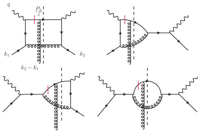
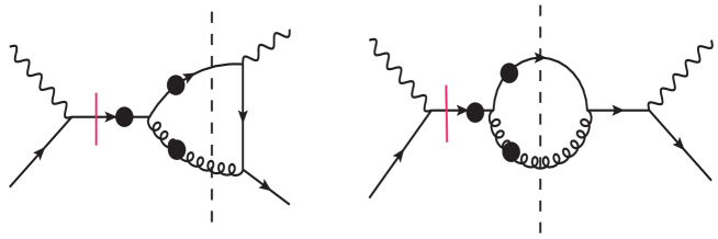
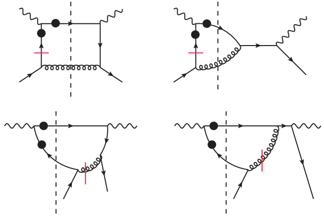
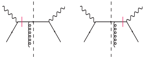
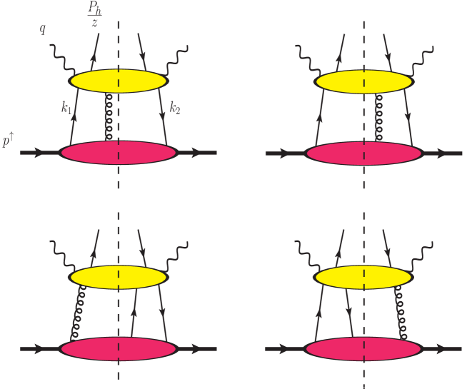
which represents the scattering of the virtual photon and the polarized proton graphically shown in Fig.1. We suppressed the Lorentz indices $\mu$ and $\nu$ of the hard parts $S^{\alpha}_{ji}(k_{1},k_{2})$ and $\tilde{S}^{\alpha}_{ji}(k_{1},k_{2})$ for simplicity. Within the collinear factorization framework, a complex phase required for the naively $T$-odd SSA can be provided by a pole contribution associated with a internal propagator. In SIDIS case, the pole contributions can be classified into four types as soft-gluon-pole(SGP), soft-fermion-pole(SFP), hard-pole(HP) and another hard-pole(HP2) which are respectively shown in Fig. 2-5. We would like to emphasize that the HP2 contribution was not considered in previous studies for the $P_{h\perp}$-weighted cross section and this contribution is essential to obtain the consistent evolution equation of $G_{F}(x_{1},x_{2})$ with the results in different approaches [22, 24, 25].

Figure 1: Diagrammatic description for the hadronic tensor $w^{\mu\nu}$. The upper diagrams and the lower diagrams respectively represent $S^{\alpha}_{ji}(k_{1},k_{2})$ and $\tilde{S}^{\alpha}_{ji}(k_{1},k_{2})$.

Figure 2: Diagrammatic description for SGP diagrams $H^{\rm SGP\,\alpha}_{Lji}(k_{1},k_{2})$. Barred propagators provide the pole contribution.

Figure 3: Diagrammatic description for HP diagrams $H^{\rm HP\,\alpha}_{Lji}(k_{1},k_{2})$. The third gluon line with momentum $k_{2}-k_{1}$ which comes from the transversely polarized proton attaches to one of the black dots in each diagram.

Figure 4: Diagrammatic description for SFP diagrams. The upper diagrams and the lower diagrams respectively represent $H^{{\rm SFP}\,\alpha}_{ji}(k_{1},k_{2})$ and $\tilde{H}^{{\rm SFP}\,\alpha}_{ji}(k_{1},k_{2})$.

Figure 5: Diagrammatic description for HP2 diagrams $H^{\rm HP2\,\alpha}_{Lji}(k_{1},k_{2})$. These diagrams were first found in [27] in the study of $P_{h\perp}$-differential SSA but was not considered in previous studies of the $P_{h\perp}$-weighted SSA.

We can check that the hard part $S^{\alpha}_{ji}(k_{1},k_{2})$ with the pole contribution satisfies the Ward identity

$$(k_{2}-k_{1})_{\alpha}S^{{\rm pole}\ \alpha}_{ji}(k_{1},k_{2}) = 0,$$ (12)

and associated relations

$$(x_{2}-x_{1}){\partial\over\partial k_{2}^{\alpha}}S^{{\rm pole}\ p}_{ji}(k_{1},k_{2})\Bigr{|}_{k_{i}=x_{i}p} = -S^{{\rm pole}\ \alpha}_{ji}(x_{1}p,x_{2}p),$$ (13)

$$(x_{2}-x_{1}){\partial\over\partial k_{1}^{\alpha}}S^{{\rm pole}\ p}_{ji}(k_{1},k_{2})\Bigr{|}_{k_{i}=x_{i}p} = S^{{\rm pole}\ \alpha}_{ji}(x_{1}p,x_{2}p).$$ (14)

For SFP and HP contributions, the above relations give

$${\partial\over\partial k_{2}^{\alpha}}S^{{\rm pole}\ p}_{ji}(k_{1},k_{2})\Bigr{|}_{k_{i}=x_{i}p}=-{\partial\over\partial k_{1}^{\alpha}}S^{{\rm pole}\ p}_{ji}(k_{1},k_{2})\Bigr{|}_{k_{i}=x_{i}p},$$ (15)

and we can find the same relation for SGP contribution with a direct inspection. Another hard part $\tilde{S}^{{\rm pole}\ p}_{ji}(k_{1},k_{2})$ also has the same relations. To extract the twist-3 $O(k_{\perp})$ contribution from the general contribution (11), we perform the collinear expansion for the hard parts as

$$S^{{\rm pole}\ \alpha}_{ji}(k_{1},k_{2}) = S^{{\rm pole}\ \alpha}_{ji}((k_{1}\cdot n)p,(k_{2}\cdot n)p)+{\partial\over\partial k_{1}^{\alpha}}S^{{\rm pole}\ p}_{ji}(k_{1},k_{2})\Bigr{|}_{k_{i}=(k_{i}\cdot n)p}\omega^{\alpha}_{\ \beta}k_{1}^{\beta}$$ (16)

$$+{\partial\over\partial k_{2}^{\alpha}}S^{{\rm pole}\ p}_{ji}(k_{1},k_{2})\Bigr{|}_{k_{i}=(k_{i}\cdot n)p}\omega^{\alpha}_{\ \beta}k_{2}^{\beta}$$

$$= S^{{\rm pole}\ \alpha}_{ji}((k_{1}\cdot n)p,(k_{2}\cdot n)p)+{\partial\over\partial k_{2}^{\alpha}}S^{{\rm pole}\ p}_{ji}(k_{1},k_{2})\Bigr{|}_{k_{i}=(k_{i}\cdot n)p}\omega^{\alpha}_{\ \beta}(k_{2}^{\beta}-k_{1}^{\beta}),\hskip 14.22636pt$$

where $\omega^{\alpha}_{\ \beta}=g^{\alpha}_{\ \beta}-p^{\alpha}n_{\beta}$ and we used the relation (15). And we separate the Lorentz components of the gluon field,

$$A^{\alpha}=A^{n}p^{\alpha}+\omega^{\alpha}_{\ \beta}A^{\beta}.$$ (17)

Then we pick up subleading contributions in (11) and construct the F-type correlator (1) as

$$w^{\mu\nu} = \int d^{4}\xi\int d^{4}\eta\int{d^{4}k_{1}\over(2\pi)^{4}}\int{d^{4}k_{2}\over(2\pi)^{4}}e^{ik_{1}\cdot\xi}e^{i\eta\cdot(k_{2}-k_{1})}\langle PS_{\perp}|\bar{\psi}_{j}(0)gA^{n}(\eta)\psi_{i}(\xi)|PS_{\perp}\rangle$$ (18)

$$\times{\partial\over\partial k_{2}^{\alpha}}\Bigl{(}S^{{\rm pole}\ p}_{ji}(k_{1},k_{2})+\tilde{S}^{{\rm pole}\ p}_{ji}(k_{1},k_{2})\Bigr{)}\Bigr{|}_{k_{i}=(k_{i}\cdot n)p}\omega^{\alpha}_{\ \beta}(k_{2}^{\beta}-k_{1}^{\beta})$$

$$+\int d^{4}\xi\int d^{4}\eta\int{d^{4}k_{1}\over(2\pi)^{4}}\int{d^{4}k_{2}\over(2\pi)^{4}}e^{ik_{1}\cdot\xi}e^{i\eta\cdot(k_{2}-k_{1})}\langle PS_{\perp}|\bar{\psi}_{j}(0)g\omega_{\alpha}^{\ \beta}A_{\beta}(\eta)\psi_{i}(\xi)|PS_{\perp}\rangle$$

$$\times\Bigl{(}S^{{\rm pole}\ p}_{ji}((k_{1}\cdot n)p,(k_{2}\cdot n)p)+\tilde{S}^{{\rm pole}\ p}_{ji}((k_{1}\cdot n)p,(k_{2}\cdot n)p)\Bigr{)}$$

$$= i\omega_{\alpha}^{\ \beta}\int dx_{1}\int dx_{2}M^{\alpha}_{ij\,F}(x_{1},x_{2}){\partial\over\partial k_{2}^{\beta}}\Bigl{(}S^{{\rm pole}\ p}_{ji}(k_{1},k_{2})+\tilde{S}^{{\rm pole}\ p}_{ji}(k_{1},k_{2})\Bigr{)}\Bigr{|}_{k_{i}=x_{i}p}$$

We express the hard parts in terms of each pole contribution as

$$S^{{\rm pole}\,\alpha}_{ji}(k_{1},k_{2}) = H^{{\rm SGP}\,\alpha}_{L\,ji}(k_{1},k_{2})\Bigl{\{}-i\pi\delta\Bigl{(}({P_{h}\over z}-(k_{2}-k_{1}))^{2}\Bigr{)}\Bigr{\}}(2\pi)\delta\Bigl{(}(k_{2}+q-{P_{h}\over z})^{2}\Bigr{)}$$ (19)

$$+H^{{\rm HP}\,\alpha}_{L\,ji}(k_{1},k_{2})\Bigl{\{}-i\pi\delta\Bigl{(}(k_{1}+q)^{2}\Bigr{)}\Bigr{\}}(2\pi)\delta\Bigl{(}(k_{2}+q-{P_{h}\over z})^{2}\Bigr{)}$$

$$+H^{{\rm SFP}\,\alpha}_{L\,ji}(k_{1},k_{2})\Bigl{\{}-i\pi\delta\Bigl{(}({P_{h}\over z}-(k_{2}-k_{1})-q)^{2}\Bigr{)}\Bigr{\}}(2\pi)\delta\Bigl{(}(k_{2}+q-{P_{h}\over z})^{2}\Bigr{)}$$

$$+{\rm mirror\ diagrams}$$

$$\tilde{S}^{{\rm pole}\,\alpha}_{ji}(k_{1},k_{2}) = \tilde{H}^{{\rm HP2}\,\alpha}_{L\,ji}(k_{1},k_{2})\Bigl{\{}i\pi\delta\Bigl{(}(k_{2}+q)^{2}\Bigr{)}\Bigr{\}}(2\pi)\delta\Bigl{(}(k_{2}-k_{1}+q-{P_{h}\over z})^{2}\Bigr{)}$$ (20)

$$+\tilde{H}^{{\rm SFP}\,\alpha}_{L\,ji}(k_{1},k_{2})\Bigl{\{}i\pi\delta\Bigl{(}({P_{h}\over z}-k_{2}-q)^{2}\Bigr{)}\Bigr{\}}(2\pi)\delta\Bigl{(}(k_{2}-k_{1}+q-{P_{h}\over z})^{2}\Bigr{)}$$

$$+{\rm mirror\ diagrams}$$

We can find that the SFP contributions $H^{{\rm SFP}\ p}_{ji}(k_{1},k_{2})$ and $\tilde{H}^{{\rm SFP}\ p}_{ji}(k_{1},k_{2})$ are the topologically same and then exactly cancel each other. After a little computation, we can obtain the formula for the hadronic tensor $W^{\mu\nu}$ as follows.

$$W^{\mu\nu} = {M_{N}\pi^{2}\over 2}\int{dz\over z^{2}}D(z)\int{dx\over x}\delta\Bigl{(}(xp+q-{P_{h}\over z})^{2}\Bigr{)}\Bigl{[}-2\epsilon^{p_{c}pnS_{\perp}}{d\over dx}G_{F}(x,x){\hat{s}+Q^{2}\over\hat{t}\hat{u}}{\rm Tr}[x{\mathchoice{\c@ncel\displaystyle{p}}{\c@ncel\textstyle{p}}{\c@ncel\scriptstyle{p}}{\c@ncel\scriptscriptstyle{p}}}H(xp)]$$ (21)

$$-2\epsilon^{p_{c}pnS_{\perp}}G_{F}(x,x){\hat{s}+Q^{2}\over\hat{t}\hat{u}}\Bigl{\{}Q^{2}\Bigl{(}{\partial\over\partial\hat{s}}-{\partial\over\partial Q^{2}}\Bigr{)}{\rm Tr}[x{\mathchoice{\c@ncel\displaystyle{p}}{\c@ncel\textstyle{p}}{\c@ncel\scriptstyle{p}}{\c@ncel\scriptscriptstyle{p}}}H(xp)]\Bigr{\}}$$

$$+G_{F}(x,x_{B}){1\over\hat{x}-1}{\hat{x}\over Q^{2}}\epsilon_{\alpha}^{\ pnS_{\perp}}\Bigl{(}{\rm Tr}[x{\mathchoice{\c@ncel\displaystyle{p}}{\c@ncel\textstyle{p}}{\c@ncel\scriptstyle{p}}{\c@ncel\scriptscriptstyle{p}}}H_{L}^{{\rm HP}\,\alpha}(x_{B}p,xp)]+{\rm Tr}[x{\mathchoice{\c@ncel\displaystyle{p}}{\c@ncel\textstyle{p}}{\c@ncel\scriptstyle{p}}{\c@ncel\scriptscriptstyle{p}}}H_{R}^{{\rm HP}\,\alpha}(xp,x_{B}p)]\Bigr{)}$$

$$-\tilde{G}_{F}(x,x_{B}){1\over\hat{x}-1}{\hat{x}\over Q^{2}}iS_{\perp\alpha}\Bigl{(}{\rm Tr}[\gamma_{5}x{\mathchoice{\c@ncel\displaystyle{p}}{\c@ncel\textstyle{p}}{\c@ncel\scriptstyle{p}}{\c@ncel\scriptscriptstyle{p}}}\tilde{H}_{L}^{{\rm HP}\,\alpha}(x_{B}p,xp)]-{\rm Tr}[\gamma_{5}x{\mathchoice{\c@ncel\displaystyle{p}}{\c@ncel\textstyle{p}}{\c@ncel\scriptstyle{p}}{\c@ncel\scriptscriptstyle{p}}}\tilde{H}_{R}^{{\rm HP}\,\alpha}(xp,x_{B}p)]$$

$$+G_{F}(x_{B},x_{B}-x){\hat{x}\over Q^{2}}\epsilon_{\alpha}^{\ pnS_{\perp}}\Bigl{(}{\rm Tr}[x{\mathchoice{\c@ncel\displaystyle{p}}{\c@ncel\textstyle{p}}{\c@ncel\scriptstyle{p}}{\c@ncel\scriptscriptstyle{p}}}H_{L}^{{\rm HP2}\,\alpha}((x_{B}-x)p,x_{B}p)]$$

$$+{\rm Tr}[x{\mathchoice{\c@ncel\displaystyle{p}}{\c@ncel\textstyle{p}}{\c@ncel\scriptstyle{p}}{\c@ncel\scriptscriptstyle{p}}}H_{R}^{{\rm HP2}\,\alpha}(x_{B}p,(x_{B}-x)p)]\Bigr{)}$$

$$-\tilde{G}_{F}(x_{B},x_{B}-x){\hat{x}\over Q^{2}}iS_{\perp\alpha}\Bigl{(}{\rm Tr}[\gamma_{5}x{\mathchoice{\c@ncel\displaystyle{p}}{\c@ncel\textstyle{p}}{\c@ncel\scriptstyle{p}}{\c@ncel\scriptscriptstyle{p}}}\tilde{H}_{L}^{{\rm HP2}\,\alpha}((x_{B}-x)p,x_{B}p)]$$

$$-{\rm Tr}[\gamma_{5}x{\mathchoice{\c@ncel\displaystyle{p}}{\c@ncel\textstyle{p}}{\c@ncel\scriptstyle{p}}{\c@ncel\scriptscriptstyle{p}}}\tilde{H}_{R}^{{\rm HP2}\,\alpha}(x_{B}p,(x_{B}-x)p)]\Bigr{]},$$

where we used the Mandelstam variables

$$\hat{s} = (xp+q)^{2}={1-\hat{x}\over\hat{x}}Q^{2},$$ (22)

$$\hat{t} = (p_{c}-q)^{2}=-{1-\hat{z}\over\hat{x}}Q^{2},$$ (23)

$$\hat{u} = (xp-p_{c})^{2}=-{\hat{z}\over\hat{x}}Q^{2},$$ (24)

where $p_{c}={P_{h}\over z}$. We used the Ward identity (13) for hard-pole contributions. For the SGP contribution, we used master formula [28, 29]

$${\partial\over\partial k_{2}^{\beta}}{\rm Tr}[x_{1}{\mathchoice{\c@ncel\displaystyle{p}}{\c@ncel\textstyle{p}}{\c@ncel\scriptstyle{p}}{\c@ncel\scriptscriptstyle{p}}}S^{{\rm SGP}\ p}_{ji}(k_{1},k_{2})]\Bigr{|}_{k_{i}=x_{i}p} = -i\pi\delta(x_{1}-x_{2}){d\over dp^{\beta}_{c}}{\rm Tr}[x_{1}{\mathchoice{\c@ncel\displaystyle{p}}{\c@ncel\textstyle{p}}{\c@ncel\scriptstyle{p}}{\c@ncel\scriptscriptstyle{p}}}S(x_{1}p)]$$ (25)

$$= 2i\pi\delta(x_{1}-x_{2}){\hat{s}+Q^{2}\over\hat{u}}p^{\beta}_{c}{\partial\over\partial\hat{t}}{\rm Tr}[x_{1}{\mathchoice{\c@ncel\displaystyle{p}}{\c@ncel\textstyle{p}}{\c@ncel\scriptstyle{p}}{\c@ncel\scriptscriptstyle{p}}}S(x_{1}p)],$$

where $S(xp)$ is the $2\to 2$ scattering cross section without the third gluon line comes from the transversely polarized proton (but the color factor is the same as $S^{SGP\,p}_{ji}$). In this paper, we consider the metric contribution,

$$L_{\mu\nu}W^{\mu\nu}\to(-g_{\mu\nu}W^{\mu\nu}),$$ (26)

$${d^{4}\langle P_{h\perp}\Delta\sigma\rangle^{\rm real}\over dx_{B}dQ^{2}dz_{h}d\phi}={\alpha^{2}_{em}\over 32\pi^{2}z_{h}x_{B}^{2}S^{2}_{ep}Q^{2}}\int{dz}zD(z)\int{d^{2}p_{c\perp}\over(2\pi)^{2}}\epsilon^{S_{\perp}p_{c\perp}pn}\Bigl{(}-g_{\mu\nu}w^{\mu\nu}\Bigr{)},$$ (27)

and the metric should be normalized as $\displaystyle g_{\mu\nu}\to{1\over 1-\epsilon}g_{\mu\nu}$ with $\epsilon=2-D/2$ in $D$-dimensional calculation. We can compute the $P_{h\perp}$-weighted cross section for NLO real-emission diagrams in $D$-dimension as follows.

$${d^{4}\langle P_{h\perp}\Delta\sigma\rangle^{\rm real}\over dx_{B}dQ^{2}dz_{h}d\phi}$$ (28)

$$= -{\pi M_{N}\alpha^{2}_{em}\alpha_{s}\over 2x_{B}^{2}S^{2}_{ep}Q^{2}}\sum_{q}e^{2}_{q}\int{dz}D^{q}(z)\mu^{2\epsilon}\int{d^{2-2\epsilon}p_{c\perp}\over(2\pi)^{2-2\epsilon}}\Bigl{[}\int{dx\over x}\delta\Bigl{(}p^{2}_{c\perp}-{(1-\hat{x})(1-\hat{z})\hat{z}\over\hat{x}}Q^{2}\Bigr{)}$$

$$\times{1\over 1-\epsilon}\Bigl{[}{d\over dx}G^{q}_{F}(x,x)H_{D}+G^{q}_{F}(x,x)H_{ND}+G^{q}_{F}(x,x_{B})H_{HP}+\tilde{G}^{q}_{F}(x,x_{B})H_{HPT}$$

$$+G^{q}_{F}(x_{B},x_{B}-x)H_{HP2}+\tilde{G}^{q}_{F}(x_{B},x_{B}-x)H_{HPT2}\Bigr{]},$$

where $q$ denotes the quark flavor, $\alpha_{s}$ is the QCD coupling constant and we used the symmetry for $p_{c\perp}$-integral

$$\int d^{2-2\epsilon}p_{c\perp}\,p_{c\perp\alpha}p_{c\perp\beta}\epsilon^{S_{\perp}\alpha pn}\epsilon^{\beta pnS_{\perp}} = -\int d^{2-2\epsilon}p_{c\perp}\,{1\over 2(1-\epsilon)}p^{2}_{c\perp}g_{\perp\alpha\beta}\epsilon^{S_{\perp}\alpha pn}\epsilon^{\beta pnS_{\perp}}$$ (29)

$$= -\int d^{2-2\epsilon}p_{c\perp}\,{1\over 2(1-\epsilon)}{(1-\hat{x})(1-\hat{z})\hat{z}\over\hat{x}}Q^{2},$$

and the hard cross sections can be computed as

$$H_{D} = {1\over 2N}\Bigl{\{}1-2\hat{x}-\hat{z}+\epsilon(1-2\hat{x}+\hat{z})+{1+\hat{x}^{2}-\epsilon(1-\hat{x})^{2}\over 1-\hat{z}}\Bigr{\}}$$ (30)

$$H_{ND} = {1\over 2N}\Bigl{[}-{2\over(1-\hat{x})(1-\hat{z})}+{1+\hat{z}+\epsilon(1-\hat{z})\over 1-\hat{x}}$$ (31)

$$+{(1-\hat{x})(1+2\hat{x})-\epsilon(1-\hat{x})(2\hat{x}-1)\over 1-\hat{z}}-2(1+\epsilon)(1-\hat{x})\Bigr{]}$$

$$H_{HP} = \Bigl{(}\hat{z}C_{F}+{1\over 2N}\Bigr{)}\Bigl{[}{2\over(1-\hat{x})(1-\hat{z})}-{1+\hat{z}+\epsilon(1-\hat{z})\over 1-\hat{x}}-{1\over 1-\hat{z}}+(1+\hat{z}+\epsilon)\Bigr{]}$$ (32)

$$H_{HPT} = {1\over 1-\epsilon}\Bigl{(}\hat{z}C_{F}+{1\over 2N}\Bigr{)}\Bigl{[}-{1+\hat{z}-2\epsilon+\epsilon^{2}(1-\hat{z})\over 1-\hat{x}}-{1+\epsilon\over 1-\hat{z}}+(1+\hat{z}+\epsilon\hat{z}+\epsilon^{2})\Bigr{]}$$ (33)

$$H_{HP2} = {1\over 2N}\Bigl{[}{1-2\hat{x}\over 1-\hat{z}}-(1-2\hat{x})(1+\hat{z}+\epsilon)\Bigr{]}+{1\over 1-\epsilon}{1\over 2}\Bigl{[}(1-2\hat{x})(2\hat{z}^{2}-2\hat{z}+1-\epsilon)\Bigr{]}$$ (34)

$$H_{HPT2} = {1\over 1-\epsilon}{1\over 2N}\Bigl{[}{1+\epsilon\over 1-\hat{z}}-(1+\hat{z}+\epsilon\hat{z}+\epsilon^{2})\Bigr{]}-{1\over 1-\epsilon}{1\over 2}\Bigl{[}1-2\hat{z}-\epsilon\Bigr{]},$$ (35)

where $N=3$ is a number of colors and $C_{F}={N^{2}-1\over 2N}$. The $p_{c\perp}$-integral can be calculated in $D$-dimension as

$$\int{d^{2-2\epsilon}p_{c}\over(2\pi)^{2-2\epsilon}}\delta\Bigl{(}p^{2}_{c\perp}-{(1-\hat{x})(1-\hat{z})\hat{z}\over\hat{x}}Q^{2}\Bigr{)}$$ (36)

$$= {1\over(2\pi)^{2-2\epsilon}}\int{dp_{c\perp}}\int d\Omega_{2-2\epsilon}(p_{c\perp})^{1-2\epsilon}\delta\Bigl{(}p^{2}_{c\perp}-{(1-\hat{x})(1-\hat{z})\hat{z}\over\hat{x}}Q^{2}\Bigr{)}$$

$$= {1\over 4\pi}\Bigl{(}{4\pi\over Q^{2}}\Bigr{)}^{\epsilon}{1\over\Gamma(1-\epsilon)}\Bigl{(}{(1-\hat{x})(1-\hat{z})\hat{z}\over\hat{x}}\Bigr{)}^{-\epsilon},$$

where $\Omega_{2-2\epsilon}$ is a solid angle

$$\int d\Omega_{2-2\epsilon}={2\pi^{1-\epsilon}\over\Gamma(1-\epsilon)}.$$ (37)

We carry out the $\epsilon$-expansion for the phase-space integral as follows.

$$\hat{z}^{-\epsilon} \simeq 1-\epsilon\ln\hat{z},\hskip 28.45274pt\hat{x}^{\epsilon}\simeq 1+\epsilon\ln\hat{z},$$ (38)

$$(1-\hat{z})^{-1-\epsilon} \simeq -{1\over\epsilon}\delta(1-\hat{z})+{1\over(1-\hat{z})_{+}}-\epsilon\Bigl{(}{\ln(1-\hat{z})\over 1-\hat{z}}\Bigr{)}_{+},$$ (39)

$$(1-\hat{x})^{-1-\epsilon} \simeq -{1\over\epsilon}\delta(1-\hat{x})+{1\over(1-\hat{x})_{+}}-\epsilon\Bigl{(}{\ln(1-\hat{x})\over 1-\hat{x}}\Bigr{)}_{+},$$ (40)

Then the cross section formula reads

$${d^{4}\langle P_{h\perp}\Delta\sigma\rangle^{\rm real}\over dx_{B}dQ^{2}dz_{h}d\phi}$$

$$= -{\pi M_{N}\alpha^{2}_{em}\over 4x_{B}^{2}S^{2}_{ep}Q^{2}}{\alpha_{s}\over 2\pi}\Bigl{(}{4\pi\mu^{2}\over Q^{2}}\Bigr{)}^{\epsilon}{1\over\Gamma(1-\epsilon)}\sum_{q}e_{q}^{2}\Bigl{[}\int dzD^{q}(z)\int{dx\over x}\Bigl{[}{d\over dx}G^{q}_{F}(x,x)\hat{\sigma}_{D}+G^{q}_{F}(x,x)\hat{\sigma}_{ND}$$

$$+G^{q}_{F}(x,x_{B})\hat{\sigma}_{HP}+\tilde{G}^{q}_{F}(x,x_{B})\hat{\sigma}_{HPT}+G^{q}_{F}(x_{B},x_{B}-x)\hat{\sigma}_{HP2}+\tilde{G}^{q}_{F}(x_{B},x_{B}-x)\hat{\sigma}_{HPT2}\Bigr{]},$$

$$\hat{\sigma}_{D} = {1\over 2N}\Bigl{[}(-{1\over\epsilon})(1+\hat{x}^{2})\delta(1-\hat{z})+(1-\hat{z})+{(1-\hat{x})^{2}+2\hat{x}\hat{z}\over(1-\hat{z})_{+}}$$ (42)

$$-\delta(1-\hat{z})\Bigl{(}(1+\hat{x}^{2})\ln{\hat{x}\over 1-\hat{x}}+2\hat{x}\Bigr{)}\Bigr{]}$$

$$\hat{\sigma}_{ND} = {1\over 2N}\Bigl{[}(-{2\over\epsilon^{2}})\delta(1-\hat{x})\delta(1-\hat{z})+(-{1\over\epsilon})\Bigl{(}2\delta(1-\hat{x})\delta(1-\hat{z})-{1+\hat{z}^{2}\over(1-\hat{z})_{+}}\delta(1-\hat{x})$$ (43)

$$+{2\hat{x}^{3}-3\hat{x}^{2}-1\over(1-\hat{x})_{+}}\delta(1-\hat{z})\Bigr{)}-2\delta(1-\hat{x})\delta(1-\hat{z})+{2\hat{x}^{3}-3\hat{x}^{2}-1\over(1-\hat{x})_{+}(1-\hat{z})_{+}}$$

$$+{1+\hat{z}\over(1-\hat{x})_{+}}-2(1-\hat{x})+\delta(1-\hat{z})\Bigl{(}-(1-\hat{x})(1+2\hat{x})\log{\hat{x}\over 1-\hat{x}}-2\Bigl{(}{\ln(1-\hat{x})\over 1-\hat{x}}\Bigr{)}_{+}$$

$$+{2\over(1-\hat{x})_{+}}-2(1-\hat{x})+2{\ln\hat{x}\over(1-\hat{x})_{+}}\Bigr{)}+\delta(1-\hat{x})\Bigl{(}(1+\hat{z})\ln\hat{z}(1-\hat{z})-2{\ln\hat{z}\over(1-\hat{z})_{+}}$$

$$-2\Bigl{(}{\ln(1-\hat{z})\over 1-\hat{z}}\Bigr{)}_{+}+{2\hat{z}\over(1-\hat{z})_{+}}\Bigr{)}\Bigr{]}$$

$$\hat{\sigma}_{HP} = \Bigl{(}\hat{z}C_{F}+{1\over 2N}\Bigr{)}\Bigl{[}{2\over\epsilon^{2}}\delta(1-\hat{x})\delta(1-\hat{z})+{1\over\epsilon}\Bigl{(}2\delta(1-\hat{x})\delta(1-\hat{z})-{1+\hat{z}^{2}\over(1-\hat{z})_{+}}\delta(1-\hat{x})$$ (44)

$$-{1+\hat{x}\over(1-\hat{x})_{+}}\delta(1-\hat{z})\Bigr{)}+2\delta(1-\hat{x})\delta(1-\hat{z})+{1+\hat{x}\hat{z}^{2}\over(1-\hat{x})_{+}(1-\hat{z})_{+}}$$

$$+\delta(1-\hat{z})\Bigl{(}\log{\hat{x}\over 1-\hat{x}}+2\Bigl{(}{\ln(1-\hat{x})\over 1-\hat{x}}\Bigr{)}_{+}-2{\ln\hat{x}\over(1-\hat{x})_{+}}-{1+\hat{x}\over(1-\hat{x})_{+}}\Bigr{)}$$

$$+\delta(1-\hat{x})\Bigl{(}-(1+\hat{z})\ln\hat{z}(1-\hat{z})+2\Bigl{(}{\ln(1-\hat{z})\over 1-\hat{z}}\Bigr{)}_{+}+2{\ln\hat{z}\over(1-\hat{z})_{+}}-{2\hat{z}\over(1-\hat{z})_{+}}\Bigr{)}\Bigr{]}$$

$$\hat{\sigma}_{HPT} = \Bigl{(}\hat{z}C_{F}+{1\over 2N}\Bigr{)}\Bigl{[}{1\over\epsilon}\delta(1-\hat{z})-{1-\hat{x}\hat{z}^{2}\over(1-\hat{x})_{+}(1-\hat{z})_{+}}+\delta(1-\hat{z})\Bigl{(}\ln{\hat{x}\over 1-\hat{x}}+3\Bigr{)}\Bigr{]}$$ (45)

$$\hat{\sigma}_{HP2} = {1\over 2N}\Bigl{[}-{1\over\epsilon}(1-2\hat{x})\delta(1-\hat{z})+{(1-2\hat{x})\hat{z}^{2}\over(1-\hat{z})_{+}}-\delta(1-\hat{z})(1-2\hat{x})(\ln{\hat{x}\over 1-\hat{x}}+1)\Bigr{]}$$ (46)

$$+{1\over 2}(1-2\hat{x})((1-\hat{z})^{2}+\hat{z}^{2})$$

$$\hat{\sigma}_{HPT2} = {1\over 2N}\Bigl{[}-{1\over\epsilon}\delta(1-\hat{z})+{\hat{z}^{2}\over(1-\hat{z})_{+}}-\delta(1-\hat{z})(\ln{\hat{x}\over 1-\hat{x}}+3)\Bigr{]}-{1\over 2}(1-2\hat{z}),$$ (47)

where we used the antisymmetric property $\tilde{G}_{F}(x,x_{B})\delta(1-\hat{x})=\tilde{G}_{F}(x,x)\delta(1-\hat{x})=0$. Finally we can derive the contribution of real-emission diagrams as

$${d^{4}\langle P_{h\perp}\Delta\sigma\rangle^{\rm real}\over dx_{B}dQ^{2}dz_{h}d\phi}$$ (48)

$$= -{z_{h}\pi M_{N}\alpha^{2}_{em}\over 4x_{B}^{2}S^{2}_{ep}Q^{2}}{\alpha_{s}\over 2\pi}\Bigl{(}{4\pi\mu^{2}\over Q^{2}}\Bigr{)}^{\epsilon}{1\over\Gamma(1-\epsilon)}\sum_{q}e_{q}^{2}\Biggl{[}C_{F}{2\over\epsilon^{2}}G^{q}_{F}(x_{B},x_{B})D^{q}(z_{h})$$

$$+\Bigl{(}-{1\over\epsilon}\Bigr{)}\Biggl{\{}D^{q}(z_{h})\Bigl{\{}\int^{1}_{x_{B}}{dx\over x}\Bigl{[}C_{F}{1+\hat{x}^{2}\over(1-\hat{x})_{+}}G^{q}_{F}(x,x)+{N\over 2}\Bigl{(}{(1+\hat{x})G^{q}_{F}(x_{B},x)-(1+\hat{x}^{2})G^{q}_{F}(x,x)\over(1-\hat{x})_{+}}$$

$$+\tilde{G}^{q}_{F}(x_{B},x)\Bigr{)}\Bigr{]}-NG^{q}_{F}(x_{B},x_{B})+{1\over 2N}\int^{1}_{x_{B}}{dx\over x}\Bigl{(}(1-2\hat{x})G^{q}_{F}(x_{B},x_{B}-x)+\tilde{G}^{q}_{F}(x_{B},x_{B}-x)\Bigr{)}\Bigr{\}}$$

$$+G^{q}_{F}(x_{B},x_{B})C_{F}\int^{1}_{z_{h}}{dz\over z}{1+\hat{z}^{2}\over(1-\hat{z})_{+}}D^{q}(z)\Biggr{\}}$$

$$+\int^{1}_{x_{B}}{dx\over x}\int^{1}_{z_{h}}{dz\over z}\Biggl{\{}x{dx\over x}G^{q}_{F}(x,x)D^{q}(z){1\over 2N\hat{z}}\Bigl{[}1-\hat{z}+{(1-\hat{x})^{2}+2\hat{x}\hat{z}\over(1-\hat{z})_{+}}$$

$$-\delta(1-\hat{z})\Bigl{(}(1+\hat{x}^{2})\ln{\hat{x}\over 1-\hat{x}}+2\hat{x}\Bigr{)}\Bigr{]}+G^{q}_{F}(x,x)D^{q}(z){1\over 2N\hat{z}}\Bigl{[}-2\delta(1-\hat{x})\delta(1-\hat{z})$$

$$+{2\hat{x}^{3}-3\hat{x}^{2}-1\over(1-\hat{x})_{+}(1-\hat{z})_{+}}+{1+\hat{z}\over(1-\hat{x})_{+}}-2(1-\hat{x})+\delta(1-\hat{z})\Bigl{(}-(1-\hat{x})(1+2\hat{x})\log{\hat{x}\over 1-\hat{x}}$$

$$-2\Bigl{(}{\ln(1-\hat{x})\over 1-\hat{x}}\Bigr{)}_{+}+{2\over(1-\hat{x})_{+}}-2(1-\hat{x})+2{\ln\hat{x}\over(1-\hat{x})_{+}}\Bigr{)}+\delta(1-\hat{x})\Bigl{(}(1+\hat{z})\ln\hat{z}(1-\hat{z})$$

$$-2{\ln\hat{z}\over(1-\hat{z})_{+}}-2\Bigl{(}{\ln(1-\hat{z})\over 1-\hat{z}}\Bigr{)}_{+}+{2\hat{z}\over(1-\hat{z})_{+}}\Bigr{)}\Bigr{]}+G^{q}_{F}(x,x_{B})D^{q}(z)\Bigl{(}C_{F}+{1\over 2N\hat{z}}\Bigr{)}\Bigl{[}2\delta(1-\hat{x})\delta(1-\hat{z})$$

$$+{1+\hat{x}\hat{z}^{2}\over(1-\hat{x})_{+}(1-\hat{z})_{+}}+\delta(1-\hat{z})\Bigl{(}\log{\hat{x}\over 1-\hat{x}}+2\Bigl{(}{\ln(1-\hat{x})\over 1-\hat{x}}\Bigr{)}_{+}-2{\ln\hat{x}\over(1-\hat{x})_{+}}-{1+\hat{x}\over(1-\hat{x})_{+}}\Bigr{)}$$

$$+\delta(1-\hat{x})\Bigl{(}-(1+\hat{z})\ln\hat{z}(1-\hat{z})+2\Bigl{(}{\ln(1-\hat{z})\over 1-\hat{z}}\Bigr{)}_{+}+2{\ln\hat{z}\over(1-\hat{z})_{+}}-{2\hat{z}\over(1-\hat{z})_{+}}\Bigr{)}\Bigr{]}$$

$$+\tilde{G}^{q}_{F}(x,x_{B})D^{q}(z)\Bigl{(}C_{F}+{1\over 2N\hat{z}}\Bigr{)}\Bigl{[}-{1-\hat{x}\hat{z}^{2}\over(1-\hat{x})_{+}(1-\hat{z})_{+}}+\delta(1-\hat{z})\Bigl{(}\ln{\hat{x}\over 1-\hat{x}}+3\Bigr{)}\Bigr{]}$$

$$+G^{q}_{F}(x_{B},x_{B}-x)D^{q}(z)\Bigl{[}{1\over 2N\hat{z}}\Bigl{(}{(1-2\hat{x})\hat{z}^{2}\over(1-\hat{z})_{+}}-\delta(1-\hat{z})(1-2\hat{x})(\ln{\hat{x}\over 1-\hat{x}}+1)\Bigr{)}$$

$$+{1\over 2\hat{z}}(1-2\hat{x})\{(1-\hat{z})^{2}+\hat{z}^{2}\}\Bigr{]}+\tilde{G}^{q}_{F}(x_{B},x_{B}-x)D^{q}(z)\Bigl{[}{1\over 2N\hat{z}}\Bigl{(}{\hat{z}^{2}\over(1-\hat{z})_{+}}$$

$$-\delta(1-\hat{z})(\ln{\hat{x}\over 1-\hat{x}}+3)\Bigr{)}-{1\over 2\hat{z}}(1-2\hat{x})\Bigr{]}\Biggr{\}}\Biggr{]},$$

where we performed partial integral,

$$\int^{1}_{x_{B}}dx{d\over dx}G_{F}(x,x)(1+\hat{x}^{2})=\int^{1}_{x_{B}}{dx\over x}G_{F}(x,x)(2\hat{x}^{2}-2\delta(1-\hat{x})),$$ (49)

and we used $G_{F}(x,x_{B})\delta(1-\hat{x})=G_{F}(x,x)\delta(1-\hat{x})$. The boundary condition of the integrals is determined by the condition $0<P_{h\perp}=\sqrt{{z^{2}(1-\hat{x})(1-\hat{z})\hat{z}\over\hat{x}}Q^{2}}<P^{\rm max}_{h\perp}$. The hard cross sections (45)-(47) associated with $\tilde{G}(x,x_{B})$, $G(x_{B},x_{B}-x)$ and $\tilde{G}(x_{B},x_{B}-x)$ are new results derived in this study and, in particular, the latter two contributions came from the HP2 contribution [27] which was not discussed in previous studies of the $P_{h\perp}$-weighted SSA. We should not neglect these new contributions to demonstrate the cancellation of the collinear singularities. Other contributions (42)-(44) agree with those derived in the previous study [26].

4 LO cross section and virtual-correction contribution in NLO cross section

In this section, we introduce the results of the LO cross section and virtual-correction contribution in NLO cross section already derived in [26]. Both contributions can be represented with $2\to 1$ scattering cross section.

Figure 6: Leading order diagram for the $P_{h\perp}$-weighted cross section. Left(Right) figure represents $S_{L(R)\gamma}(k_{1},k_{2})$.

The phase-space integral should be changed from $2\to 2$ scattering as follows.

$${d^{3}p_{c}\over(2\pi)^{3}2p^{0}_{c}}{d^{3}p_{d}\over(2\pi)^{3}2p^{0}_{d}}(2\pi)^{4}\delta^{4}(xp+q-p_{c}-p_{d})$$ (50)

$$= {d^{3}p_{c}\over(2\pi)^{3}2p^{0}_{c}}(2\pi)\delta\Bigl{(}(xp+q-p_{c})^{2}\Bigr{)}$$

$$\to {d^{3}p_{c}\over(2\pi)^{3}2p^{0}_{c}}(2\pi)^{4}\delta^{4}(xp+q-p_{c})$$

In this case, we perform $P_{h\perp}$-integration before the collinear expansion as

$$\int d^{2}P_{h\perp}\epsilon^{\alpha\beta pn}S_{\perp\alpha}P_{h\perp\beta}\Bigl{(}S_{L\gamma}(k_{1},k_{2})\delta^{2}(k_{2\perp}-{P_{h\perp}\over z})+S_{R\gamma}(k_{1},k_{2})\delta^{2}(k_{1\perp}-{P_{h\perp}\over z})\Bigr{)}$$ (51)

$$= \epsilon^{\alpha\beta pn}S_{\perp\alpha}z^{3}\Bigl{(}k_{2\perp\beta}S_{L\gamma}(k_{1},k_{2})+k_{1\perp\beta}S_{R\gamma}(k_{1},k_{2})\Bigr{)},$$

where we used the fact the virtual photon doesn’t have transverse momentum in hadron frame. We can find the following relation for LO diagram shown in Fig.6.

$$S_{Lp}(x_{1}p,x_{2}p)=-S_{Rp}(x_{1}p,x_{2}p)\equiv S_{p}(x_{1}p,x_{2}p).$$ (52)

Since the $P_{h\perp}$-integration brought $O(k_{\perp})$ term, the leading term of the collinear expansion gives twist-3 contribution. We can construct the gluon’s field strength tensor as follows.

$$\int{d^{4}k_{1}\over(2\pi)^{4}}\int{d^{4}k_{2}\over(2\pi)^{4}}e^{ik_{1}\cdot\xi}e^{i(k_{2}-k_{1})\cdot\eta}A^{n}(\eta)(k_{2\perp\beta}-k_{1\perp\beta})S_{p}((k_{1}\cdot n)p,(k_{2}\cdot n)p)$$ (53)

$$= i\int{d^{4}k_{1}\over(2\pi)^{4}}\int{d^{4}k_{2}\over(2\pi)^{4}}e^{ik_{1}\cdot\xi}e^{i(k_{2}-k_{1})\cdot\eta}F_{\beta}^{\ n}(\eta)S_{p}((k_{1}\cdot n)p,(k_{2}\cdot n)p)$$

$$+\int{d^{4}k_{1}\over(2\pi)^{4}}\int{d^{4}k_{2}\over(2\pi)^{4}}e^{ik_{1}\cdot\xi}e^{i(k_{2}-k_{1})\cdot\eta}A^{\perp}_{\beta}(\eta)(k_{2}\cdot n-k_{1}\cdot n)S_{p}((k_{1}\cdot n)p,(k_{2}\cdot n)p).$$

The last term vanishes due to the SGP delta function. Then we can use the following formula for LO contribution

$${d^{4}\langle P_{h\perp}\Delta\sigma\rangle^{\rm LO}\over dx_{B}dQ^{2}dz_{h}d\phi} = {\alpha^{2}_{em}\over 8z_{h}x_{B}^{2}S^{2}_{ep}Q^{2}}\int dzzD(z)\int dx_{1}\int dx_{2}\epsilon^{S_{\perp}\alpha pn}iM_{Fij\,\alpha}(x_{1},x_{2})$$ (54)

$$\times\Bigl{(}-g_{\mu\nu}H_{ij\,p}^{\mu\nu}(x_{1}p,x_{2}p)\Bigr{)}\Bigl{(}{-2x\hat{x}\over\hat{u}Q^{2}}\Bigr{)}\delta(x_{1}-x_{2})\delta(1-\hat{x})\delta(1-\hat{z}),$$

which agrees with the corresponding formula in [21, 26]. LO and NLO contributions in SIDIS were already calculated in previous work [26]. We just introduce their results in our notation below.

$${d^{4}\langle P_{h\perp}\Delta\sigma\rangle^{\rm LO}\over dx_{B}dQ^{2}dz_{h}d\phi}=-{z_{h}\pi M_{N}\alpha^{2}_{em}\over 4x_{B}^{2}S^{2}_{ep}Q^{2}}\sum_{q}e^{2}_{q}G^{q}(x_{B},x_{B})D^{q}(z_{h})$$ (55)

$${d^{4}\langle P_{h\perp}\Delta\sigma\rangle^{\rm virtual}\over dx_{B}dQ^{2}dz_{h}d\phi} = -{z_{h}\pi M_{N}\alpha^{2}_{em}\over 4x_{B}^{2}S^{2}_{ep}Q^{2}}{\alpha_{s}\over 2\pi}\sum_{q}e_{q}^{2}G^{q}(x_{B},x_{B})D^{q}(z_{h})$$ (56)

$$\times\Bigl{[}C_{F}\Bigr{(}{4\pi\mu^{2}\over Q^{2}}\Bigr{)}^{\epsilon}{1\over\Gamma(1-\epsilon)}\Bigl{(}-{2\over\epsilon^{2}}-{3\over\epsilon}-8\Bigr{)}\Bigr{]}$$

Combining (48), (55) and (56), we obtain the following complete formula for NLO $P_{h\perp}$-weighted cross section.

$${d^{4}\langle P_{h\perp}\Delta\sigma\rangle^{\rm LO+NLO}\over dx_{B}dQ^{2}dz_{h}d\phi}$$ (57)

$$= -{\pi z_{h}M_{N}\alpha^{2}_{em}\over 4x_{B}^{2}S^{2}_{ep}Q^{2}}\sum_{q}e_{q}^{2}\Biggl{[}G^{q}_{F}(x_{B},x_{B})D^{q}(z_{h})+{\alpha_{s}\over 2\pi}\Bigl{(}{4\pi\mu^{2}\over Q^{2}}\Bigr{)}^{\epsilon}{1\over\Gamma(1-\epsilon)}\Bigl{(}-{1\over\epsilon}\Bigr{)}$$

$$\times\Biggl{\{}D^{q}(z_{h})\Bigl{\{}\int^{1}_{x_{B}}{dx\over x}\Bigl{[}P_{qq}(\hat{x})G^{q}_{F}(x,x)+{N\over 2}\Bigl{(}{(1+\hat{x})G^{q}_{F}(x_{B},x)-(1+\hat{x}^{2})G^{q}_{F}(x,x)\over(1-\hat{x})_{+}}+\tilde{G}^{q}_{F}(x_{B},x)\Bigr{)}\Bigr{]}$$

$$-NG^{q}_{F}(x_{B},x_{B})+{1\over 2N}\int^{1}_{x_{B}}{dx\over x}\Bigl{(}(1-2\hat{x})G^{q}_{F}(x_{B},x_{B}-x)+\tilde{G}^{q}_{F}(x_{B},x_{B}-x)\Bigr{)}\Bigr{\}}$$

$$+G^{q}_{F}(x_{B},x_{B})\int^{1}_{z_{h}}{dz\over z}P_{qq}(\hat{z})D^{q}(z)\Biggr{\}}$$

$$+{\alpha_{s}\over 2\pi}\Bigl{(}{4\pi\mu^{2}\over Q^{2}}\Bigr{)}^{\epsilon}{1\over\Gamma(1-\epsilon)}\int^{1}_{x_{B}}{dx\over x}\int^{1}_{z_{h}}{dz\over z}\Biggl{\{}x{dx\over x}G^{q}_{F}(x,x)D^{q}(z){1\over 2N\hat{z}}\Bigl{[}1-\hat{z}+{(1-\hat{x})^{2}+2\hat{x}\hat{z}\over(1-\hat{z})_{+}}$$

$$-\delta(1-\hat{z})\Bigl{(}(1+\hat{x}^{2})\ln{\hat{x}\over 1-\hat{x}}+2\hat{x}\Bigr{)}\Bigr{]}+G^{q}_{F}(x,x)D^{q}(z){1\over 2N\hat{z}}\Bigl{[}-2\delta(1-\hat{x})\delta(1-\hat{z})$$

$$+{2\hat{x}^{3}-3\hat{x}^{2}-1\over(1-\hat{x})_{+}(1-\hat{z})_{+}}+{1+\hat{z}\over(1-\hat{x})_{+}}-2(1-\hat{x})+\delta(1-\hat{z})\Bigl{(}-(1-\hat{x})(1+2\hat{x})\log{\hat{x}\over 1-\hat{x}}$$

$$-2\Bigl{(}{\ln(1-\hat{x})\over 1-\hat{x}}\Bigr{)}_{+}+{2\over(1-\hat{x})_{+}}-2(1-\hat{x})+2{\ln\hat{x}\over(1-\hat{x})_{+}}\Bigr{)}+\delta(1-\hat{x})\Bigl{(}(1+\hat{z})\ln\hat{z}(1-\hat{z})$$

$$-2{\ln\hat{z}\over(1-\hat{z})_{+}}-2\Bigl{(}{\ln(1-\hat{z})\over 1-\hat{z}}\Bigr{)}_{+}+{2\hat{z}\over(1-\hat{z})_{+}}\Bigr{)}\Bigr{]}+G^{q}_{F}(x,x_{B})D^{q}(z)\Bigl{(}C_{F}+{1\over 2N\hat{z}}\Bigr{)}\Bigl{[}2\delta(1-\hat{x})\delta(1-\hat{z})$$

$$+{1+\hat{x}\hat{z}^{2}\over(1-\hat{x})_{+}(1-\hat{z})_{+}}+\delta(1-\hat{z})\Bigl{(}\log{\hat{x}\over 1-\hat{x}}+2\Bigl{(}{\ln(1-\hat{x})\over 1-\hat{x}}\Bigr{)}_{+}-2{\ln\hat{x}\over(1-\hat{x})_{+}}-{1+\hat{x}\over(1-\hat{x})_{+}}\Bigr{)}$$

$$+\delta(1-\hat{x})\Bigl{(}-(1+\hat{z})\ln\hat{z}(1-\hat{z})+2\Bigl{(}{\ln(1-\hat{z})\over 1-\hat{z}}\Bigr{)}_{+}+2{\ln\hat{z}\over(1-\hat{z})_{+}}-{2\hat{z}\over(1-\hat{z})_{+}}\Bigr{)}\Bigr{]}$$

$$+\tilde{G}^{q}_{F}(x,x_{B})D^{q}(z)\Bigl{(}C_{F}+{1\over 2N\hat{z}}\Bigr{)}\Bigl{[}-{1-\hat{x}\hat{z}^{2}\over(1-\hat{x})_{+}(1-\hat{z})_{+}}+\delta(1-\hat{z})\Bigl{(}\ln{\hat{x}\over 1-\hat{x}}+3\Bigr{)}\Bigr{]}$$

$$+G^{q}_{F}(x_{B},x_{B}-x)D^{q}(z)\Bigl{[}{1\over 2N\hat{z}}\Bigl{(}{(1-2\hat{x})\hat{z}^{2}\over(1-\hat{z})_{+}}-\delta(1-\hat{z})(1-2\hat{x})(\ln{\hat{x}\over 1-\hat{x}}+1)\Bigr{)}$$

$$+{1\over 2\hat{z}}(1-2\hat{x})\{(1-\hat{z})^{2}+\hat{z}^{2}\}\Bigr{]}+\tilde{G}^{q}_{F}(x_{B},x_{B}-x)D^{q}(z)\Bigl{[}{1\over 2N\hat{z}}\Bigl{(}{\hat{z}^{2}\over(1-\hat{z})_{+}}$$

$$-\delta(1-\hat{z})(\ln{\hat{x}\over 1-\hat{x}}+3)\Bigr{)}-{1\over 2\hat{z}}(1-2\hat{x})\Bigr{]}-8C_{F}\delta(1-\hat{x})\delta(1-\hat{z})\Biggr{\}}\Biggr{]},$$

where $P_{qq}(x)$ is the splitting function

$$P_{qq}(x)=C_{F}\Bigl{[}{1+x^{2}\over(1-x)_{+}}+{3\over 2}\delta(1-x)\Bigr{]}.$$ (58)

The double pole terms ${2\over\epsilon^{2}}\delta(1-\hat{x})\delta(1-\hat{z})$ are cancelled between the real cross section and the virtual cross section. The single pole term in virtual cross section $2\times{3\over 2}\delta(1-\hat{x})\delta(1-\hat{z})$ is incorporated into the splitting functions. The collinear singularities associated with the twist-3 functions can be subtracted with the following renormalization.

$$G_{F}(x_{B},x_{B})$$ (59)

$$= G^{(0)}_{F}(x_{B},x_{B})+{\alpha_{s}\over 2\pi}\Bigr{(}-{1\over\hat{\epsilon}}\Bigr{)}\Bigl{\{}\int^{1}_{x_{B}}{dx\over x}\Bigl{[}P_{qq}(\hat{x})G_{F}(x,x)$$

$$+{N\over 2}\Bigl{(}{(1+\hat{x})G_{F}(x_{B},x)-(1+\hat{x}^{2})G_{F}(x,x)\over(1-\hat{x})_{+}}+\tilde{G}_{F}(x_{B},x)\Bigr{)}\Bigr{]}-NG_{F}(x_{B},x_{B})$$

$$+{1\over 2N}\int^{1}_{x_{B}}{dx\over x}\Bigl{(}(1-2\hat{x})G_{F}(x_{B},x_{B}-x)+\tilde{G}_{F}(x_{B},x_{B}-x)\Bigr{)}\Bigr{\}},$$

where we adopted the $\overline{{\rm MS}}$-scheme

$${1\over\hat{\epsilon}}={1\over\epsilon}-\gamma_{E}+\ln 4\pi.$$ (60)

These collinear singularities are the same as those in F-type correlator (1) at 1-loop order [22, 24, 25]. Then the collinear singularities are consistently subtracted and we can obtain the infrared-safe NLO cross section as follows.

$${d^{4}\langle P_{h\perp}\Delta\sigma\rangle^{\rm LO+NLO}\over dx_{B}dQ^{2}dz_{h}d\phi}$$ (61)

$$= -{\pi z_{h}M_{N}\alpha^{2}_{em}\over 4x_{B}^{2}S^{2}_{ep}Q^{2}}\sum_{q}e_{q}^{2}\Biggl{[}G^{q}_{F}(x_{B},x_{B},\mu)D^{q}(z_{h},\mu)$$

$$+{\alpha_{s}\over 2\pi}\ln\Bigl{(}{Q^{2}\over\mu^{2}}\Bigr{)}\Biggl{\{}D^{q}(z_{h},\mu)\Bigl{\{}\int^{1}_{x_{B}}{dx\over x}\Bigl{[}P_{qq}(\hat{x})G^{q}_{F}(x,x,\mu)$$

$$+{N\over 2}\Bigl{(}{(1+\hat{x})G^{q}_{F}(x_{B},x,\mu)-(1+\hat{x}^{2})G^{q}_{F}(x,x,\mu)\over(1-\hat{x})_{+}}+\tilde{G}^{q}_{F}(x_{B},x,\mu)\Bigr{)}\Bigr{]}$$

$$-NG^{q}_{F}(x_{B},x_{B},\mu)+{1\over 2N}\int^{1}_{x_{B}}{dx\over x}\Bigl{(}(1-2\hat{x})G^{q}_{F}(x_{B},x_{B}-x,\mu)+\tilde{G}^{q}_{F}(x_{B},x_{B}-x,\mu)\Bigr{)}\Bigr{\}}$$

$$+G^{q}_{F}(x_{B},x_{B},\mu)\int^{1}_{z_{h}}{dz\over z}P_{qq}(\hat{z})D^{q}(z,\mu)\Biggr{\}}$$

$$+{\alpha_{s}\over 2\pi}\int^{1}_{x_{B}}{dx\over x}\int^{1}_{z_{h}}{dz\over z}\Biggl{\{}x{dx\over x}G^{q}_{F}(x,x,\mu)D^{q}(z,\mu){1\over 2N\hat{z}}\Bigl{[}1-\hat{z}+{(1-\hat{x})^{2}+2\hat{x}\hat{z}\over(1-\hat{z})_{+}}$$

$$-\delta(1-\hat{z})\Bigl{(}(1+\hat{x}^{2})\ln{\hat{x}\over 1-\hat{x}}+2\hat{x}\Bigr{)}\Bigr{]}+G^{q}_{F}(x,x,\mu)D^{q}(z,\mu){1\over 2N\hat{z}}\Bigl{[}-2\delta(1-\hat{x})\delta(1-\hat{z})$$

$$+{2\hat{x}^{3}-3\hat{x}^{2}-1\over(1-\hat{x})_{+}(1-\hat{z})_{+}}+{1+\hat{z}\over(1-\hat{x})_{+}}-2(1-\hat{x})+\delta(1-\hat{z})\Bigl{(}-(1-\hat{x})(1+2\hat{x})\log{\hat{x}\over 1-\hat{x}}$$

$$-2\Bigl{(}{\ln(1-\hat{x})\over 1-\hat{x}}\Bigr{)}_{+}+{2\over(1-\hat{x})_{+}}-2(1-\hat{x})+2{\ln\hat{x}\over(1-\hat{x})_{+}}\Bigr{)}+\delta(1-\hat{x})\Bigl{(}(1+\hat{z})\ln\hat{z}(1-\hat{z})$$

$$-2{\ln\hat{z}\over(1-\hat{z})_{+}}-2\Bigl{(}{\ln(1-\hat{z})\over 1-\hat{z}}\Bigr{)}_{+}+{2\hat{z}\over(1-\hat{z})_{+}}\Bigr{)}\Bigr{]}$$

$$+G^{q}_{F}(x,x_{B},\mu)D^{q}(z,\mu)\Bigl{(}C_{F}+{1\over 2N\hat{z}}\Bigr{)}\Bigl{[}2\delta(1-\hat{x})\delta(1-\hat{z})+{1+\hat{x}\hat{z}^{2}\over(1-\hat{x})_{+}(1-\hat{z})_{+}}$$

$$+\delta(1-\hat{z})\Bigl{(}\log{\hat{x}\over 1-\hat{x}}+2\Bigl{(}{\ln(1-\hat{x})\over 1-\hat{x}}\Bigr{)}_{+}-2{\ln\hat{x}\over(1-\hat{x})_{+}}-{1+\hat{x}\over(1-\hat{x})_{+}}\Bigr{)}$$

$$+\delta(1-\hat{x})\Bigl{(}-(1+\hat{z})\ln\hat{z}(1-\hat{z})+2\Bigl{(}{\ln(1-\hat{z})\over 1-\hat{z}}\Bigr{)}_{+}+2{\ln\hat{z}\over(1-\hat{z})_{+}}-{2\hat{z}\over(1-\hat{z})_{+}}\Bigr{)}\Bigr{]}$$

$$+\tilde{G}^{q}_{F}(x,x_{B},\mu)D^{q}(z,\mu)\Bigl{(}C_{F}+{1\over 2N\hat{z}}\Bigr{)}\Bigl{[}-{1-\hat{x}\hat{z}^{2}\over(1-\hat{x})_{+}(1-\hat{z})_{+}}+\delta(1-\hat{z})\Bigl{(}\ln{\hat{x}\over 1-\hat{x}}+3\Bigr{)}\Bigr{]}$$

$$+G^{q}_{F}(x_{B},x_{B}-x,\mu)D^{q}(z,\mu)\Bigl{[}{1\over 2N\hat{z}}\Bigl{(}{(1-2\hat{x})\hat{z}^{2}\over(1-\hat{z})_{+}}-\delta(1-\hat{z})(1-2\hat{x})(\ln{\hat{x}\over 1-\hat{x}}+1)\Bigr{)}$$

$$+{1\over 2\hat{z}}(1-2\hat{x})\{(1-\hat{z})^{2}+\hat{z}^{2}\}\Bigr{]}+\tilde{G}^{q}_{F}(x_{B},x_{B}-x,\mu)D^{q}(z,\mu)\Bigl{[}{1\over 2N\hat{z}}\Bigl{(}{\hat{z}^{2}\over(1-\hat{z})_{+}}$$

$$-\delta(1-\hat{z})(\ln{\hat{x}\over 1-\hat{x}}+3)\Bigr{)}-{1\over 2\hat{z}}(1-2\hat{x})\Bigr{]}-8C_{F}\delta(1-\hat{x})\delta(1-\hat{z})\Biggr{\}}\Biggr{]}+O(\alpha^{2}_{s}),$$

where the scale dependence of $G_{F}(x,x,\mu^{2})$ was introduced so that the cross section doesn’t depend on the artificial scale $\mu$. Then we can derive the scale evolution equation of $G_{F}(x,x,\mu^{2})$ as

$${\partial\over\partial\ln\mu^{2}}{d^{4}\langle P_{h\perp}\Delta\sigma\rangle^{\rm LO+NLO}\over dx_{B}dQ^{2}dz_{h}d\phi}=0$$

$$\to{\partial\over\partial\ln\mu^{2}}G_{F}(x_{B},x_{B},\mu^{2})={\alpha_{s}\over 2\pi}\Bigl{\{}\int^{1}_{x_{B}}{dx\over x}\Bigl{[}P_{qq}(\hat{x})G_{F}(x,x,\mu^{2})$$

$$+{N\over 2}\Bigl{(}{(1+\hat{x})G_{F}(x_{B},x,\mu^{2})-(1+\hat{x}^{2})G_{F}(x,x,\mu^{2})\over(1-\hat{x})_{+}}+\tilde{G}_{F}(x_{B},x,\mu^{2})\Bigr{)}\Bigr{]}-NG_{F}(x_{B},x_{B},\mu^{2})$$

$$+{1\over 2N}\int^{1}_{x_{B}}{dx\over x}\Bigl{(}(1-2\hat{x})G_{F}(x_{B},x_{B}-x,\mu^{2})+\tilde{G}_{F}(x_{B},x_{B}-x,\mu^{2})\Bigr{)}\Bigr{\}}+O(\alpha^{2}_{s}),$$ (62)

which completely agrees with the results in [22, 24, 25].

5 Summary

We added the new hard pole contribution to the $P_{h\perp}$-weighted single-spin asymmetry in semi-inclusive deep inelastic scattering. Since the new pole contribution brings some collinear singularities at one-loop order, we should not neglect it for the exact cancellation of the collinear singularities. Our result showed that the NLO $P_{h\perp}$-weighted cross section has the same collinear singularities with the F-type correlator at one-loop order and then the singularities can be subtracted consistently. In addition, our calculation provided the scale evolution equation of the Qiu-Sterman function which completely agrees with the corresponding results in different approaches.

References

• [1] R. D. Klem, J. E. Bowers, H. W. Courant, H. Kagan, M. L. Marshak, E. A. Peterson, K. Ruddick and W. H. Dragoset et al., Phys. Rev. Lett.  36, 929 (1976).
• [2] G. Bunce et al., Phys. Rev. Lett.  36, 1113 (1976).
• [3] A. V. Efremov and O. V. Teryaev, Sov. J. Nucl. Phys.  36, 140 (1982) [Yad. Fiz.  36, 242 (1982)]; Phys. Lett. B 150, 383 (1985).
• [4] J.-w. Qiu and G. F. Sterman, Phys. Rev. Lett.  67, 2264 (1991).
• [5] J.-w. Qiu and G. F. Sterman, Nucl. Phys. B 378, 52 (1992).
• [6] J.-w. Qiu and G. F. Sterman, Phys. Rev. D 59, 014004 (1999) [hep-ph/9806356].
• [7] Y. Kanazawa and Y. Koike, Phys. Rev. D 64, 034019 (2001) [hep-ph/0012225].
• [8] X. Ji, J.-w. Qiu, W. Vogelsang and F. Yuan, Phys. Rev. D 73, 094017 (2006) [hep-ph/0604023].
• [9] X. Ji, J.-w. Qiu, W. Vogelsang and F. Yuan, Phys. Lett. B 638, 178 (2006) [hep-ph/0604128].
• [10] C. Kouvaris, J. W. Qiu, W. Vogelsang and F. Yuan, Phys. Rev.  D 74, 114013 (2006) [arXiv:hep-ph/0609238].
• [11] H. Eguchi, Y. Koike and K. Tanaka, Nucl. Phys. B 763, 198-227 (2007) [arXiv:hep-ph/0610314].
• [12] Z. B. Kang and J. W. Qiu, Phys. Rev. D 78, 034005 (2008) [arXiv:hep-ph/0806.1970]: Z. B. Kang, J. W. Qiu, W. Vogelsang and F. Yuan, Phys. Rev. D 78, 114013 (2008) [arXiv:hep-ph/0810.3333]
• [13] F. Yuan and J. Zhou, Phys. Rev. Lett.  103, 052001 (2009) [arXiv:0903.4680 [hep-ph]].
• [14] Z. B. Kang, F. Yuan and J. Zhou, Phys. Lett. B 691, 243 (2010) [arXiv:1002.0399 [hep-ph]].
• [15] H. Beppu, Y. Koike, K. Tanaka and S. Yoshida, Phys. Rev. D 82, 054005 (2010) [arXiv:1007.2034 [hep-ph]].
• [16] A. Metz and D. Pitonyak, Phys. Lett. B 723, 365 (2013) [arXiv:1212.5037 [hep-ph]].
• [17] K. Kanazawa and Y. Koike, Phys. Rev. D 88, 074022 (2013) [arXiv:1309.1215 [hep-ph]].
• [18] K. Kanazawa and Y. Koike, Phys. Rev. D 82, 034009 (2010) [arXiv:1005.1468 [hep-ph]]; Phys. Rev. D 83, 114024 (2011) [arXiv:1104.0117 [hep-ph]].
• [19] Z. B. Kang and J. W. Qiu, Phys. Rev. D 79, 016003 (2009) [arXiv:0811.3101 [hep-ph]].
• [20] J. Zhou, F. Yuan and Z. T. Liang, Phys. Rev. D 79, 114022 (2009) [arXiv:0812.4484 [hep-ph]].
• [21] W. Vogelsang and F. Yuan, Phys. Rev. D 79, 094010 (2009) [arXiv:0904.0410 [hep-ph]].
• [22] V. M. Braun, A. N. Manashov and B. Pirnay, Phys. Rev. D 80, 114002 (2009) [arXiv:0909.3410 [hep-ph]].
• [23] A. Schafer and J. Zhou, Phys. Rev. D 85, 117501 (2012) [arXiv:1203.5293 [hep-ph]].
• [24] J. P. Ma and Q. Wang, Phys. Lett. B 715, 157 (2012) [arXiv:1205.0611 [hep-ph]].
• [25] Z. B. Kang and J. W. Qiu, Phys. Lett. B 713, 273 (2012) [arXiv:1205.1019 [hep-ph]].
• [26] Z. B. Kang, I. Vitev and H. Xing, Phys. Rev. D 87, 034024 (2013) [arXiv:1212.1221 [hep-ph]].
• [27] Y. Koike and K. Tanaka, arXiv:0907.2797 [hep-ph].
• [28] Y. Koike, K. Tanaka and S. Yoshida, Phys. Rev. D 83, 114014 (2011) [arXiv:1104.0798 [hep-ph]].
• [29] Y. Koike and K. Tanaka, Phys. Lett. B 646, 232 (2007) [Erratum-ibid. B 668, 458 (2008)] [hep-ph/0612117].