A conjugate gradient method for electronic structure calculations

Abstract

In this paper, we study a conjugate gradient method for electronic structure calculations. We propose a Hessian based step size strategy, which together with three orthogonality approaches yields three algorithms for computing the ground state energy of atomic and molecular systems. Under some mild assumptions, we prove that our algorithms converge locally. It is shown by our numerical experiments that the conjugate gradient method is efficient.

mmsxxxxxxxx–x

1 Introduction

Kohn-Sham density functional theory (DFT) [15, 18, 22] is widely used in electronic structure calculations. It is often formulated as a nonlinear eigenvalue problem or a direct minimization problem under orthogonality constraint [5, 21, 26].

The nonlinear eigenvalue problem is usually solved by using the self consistent field (SCF) iterations, by which the central computation in solving such nonlinear eigenvalue problems is the repeated solution of some algebraic eigenvalue problems. However, the convergence of SCF is not guaranteed, especially for large scale systems with small band gaps, for which the performance of the SCF iterations is unpredictable [41, 42].

Therefore, people turn to investigate constrained minimization approaches for the Kohn-Sham direct energy minimization models, see e.g. [11, 12, 27, 34, 35, 38, 39, 41, 42] and references therein. In [41], the authors constructed the search direction from the subspace spanned by the current orbital approximations, the associated preconditioned gradient, and the previous search direction. The optimal search direction and step size are computed by solving a smaller scale nonlinear eigenvalue problem, which is complicated for large systems. While the authors in [39, 42] applied gradient type methods to the minimization problem, in which the gradient is chosen as the search direction. It has been shown in [42] that the gradient type methods are quite efficient and can outperform the SCF iterations on many practical systems.

We should point out that there are also several works using some conjugate gradient (CG) methods to the electronic structure calculations, see e.g., [23, 31, 33]. However, in these works, their starting points are to solve the nonlinear eigenvalue problems other than the minimization problems, the CG methods are used to find the subspaces by updating each orbital along its corresponding conjugate gradient direction, and these orbitals are updated successively. After all the orbitals are updated, a subspace diagonalization (Rayleigh-Ritz) procedure is then carried out. As pointed out in [41], due to the “band-by-band” nature, the algorithms are not very efficient.

In this paper, following [39, 42], we apply the similar idea to construct some novel conjugate gradient method, where the search direction is replaced by the conjugate gradient direction. We utilize the so-called WY [39] and QR strategies to keep the orthogonality of the Kohn-Sham orbitals, which were also employed in [42]. In addition, we also apply the polar decomposition (PD) [2] based approach to do the orthogonalization.

We understand that an important issue in a conjugate gradient method is the choice of step size. To set up the step size in our conjugate gradient method, we introduce a Hessian based strategy, which is based on the local second order Taylor expansion of the total energy functional. We prove the convergence of the WY, QR, and PD based conjugate gradient algorithms, and observe that the QR based conjugate gradient algorithm usually performs best in our numerical experiments. Although we need some energy descent property, which is widely used in many optimization algorithms, to prove the convergence of the algorithms theoretically (see Theorem 16), our algorithms perform well without using any backtracking procedure. We compare our algorithms with the algorithm OptM-QR recently proposed in [42] which is a gradient type method with Barzilai-Borwein (BB) step sizes, and observe from our numerical experiments that our algorithms need less iterations and less computational time to obtain the results with same accuracy. In addition, it is shown by our numerical experiments that the algorithm OptM-QR is less stable than our algorithms, which may be caused by the nonmonotonic behavior of the BB step size [6].

We see that the standard Armijo and the exact line search strategies are applied to the geometric CG method on matrix manifold (see Algorithm 13 of [2]). However, the exact line search is not recommended to the Kohn-Sham total energy minimization problem due to its high computational cost. Note that the Armijo line search method uses a fixed initial value and performs a backtracking procedure to ensure some energy decent property. We believe that our Hessian based strategy is more efficient in providing a good initial value for the step size and reducing the times of backtracking. In particular, there is no convergence analysis for Algorithm 13 given in [2]. We point out that Smith [29, 30] has also proposed a CG algorithm on the Riemannian manifold, where the orthogonality was preserved by using the Riemannian exponential map, whose computational cost is larger than the WY, QR, and PD strategies.

We should mention that the convergence of SCF iteration was proved in [19, 20, 40] under the assumptions that the gap between the occupied states and unoccupied states is sufficiently large and the second-order derivatives of the exchange correlation functional are uniformly bounded from above. Anyway, such investigations are theoretically significant.

The rest of this paper is organized as follows: in Section 2, we provide a brief introduction to the Kohn-Sham model and the associated Grassmann manifold. We then propose our conjugate gradient algorithms in Section 3 and prove the convergence of the three algorithms in Section 4. In Section 5, we present some restarted versions of our algorithms. We report several numerical experiments in Section 6 that demonstrate the accuracy and efficiency of our algorithms. After that, we give some concluding remarks in Section 7. Finally, we provide the proof of Lemma 6 in Appendix A and present several numerical tests using different step sizes and different calculation formulas for the Hessian in Appendix B that lead to our recommendations.

2 Preliminaries

2.1 Kohn-Sham model

By Kohn-Sham density functional theory, the ground state of a system consisting of $M$ nuclei of charges and $N$ electrons can be obtained by solving the following constrained optimization problem

(1) $$\begin{split}&\inf_{U=(u_{1},\dots,u_{N})\in(H^{1}(\mathbb{R}^{3}))^{N}}\ \ \ \ \ \ \ E(U)\\ s.t.&\int_{\mathbb{R}^{3}}u_{i}u_{j}=\delta_{ij},1\leq i,j\leq N,\end{split}$$

where the Kohn-Sham total energy $E(U)$ is defined by

(2) $$E(U) = \frac{1}{2}\int_{\mathbb{R}^{3}}\sum_{i=1}^{N}|\nabla u_{i}(r)|^{2}dr+\frac{1}{2}\int_{\mathbb{R}^{3}}\int_{\mathbb{R}^{3}}\frac{\rho(r)\rho(r^{\prime})}{|r-r^{\prime}|}drdr^{\prime}$$

$$+\int_{\mathbb{R}^{3}}\sum_{i=1}^{N}u_{i}(r)V_{ext}(r)u_{i}(r)dr+\int_{\mathbb{R}^{3}}\varepsilon_{xc}(\rho)(r)\rho(r)dr,$$

and $u_{i}\in H^{1}(\mathbb{R}^{3}),i=1,\cdots,N$ are the Kohn-Sham orbitals. Here $\rho(r)=\sum\limits_{i=1}^{N}|u_{i}(r)|^{2}$ is the electronic density, $V_{ext}(r)$ is the external potential generated by the nuclei: for full potential calculations, $V_{ext}(r)=-\sum\limits_{I=1}^{M}\frac{Z_{I}}{|r-R_{I}|}$, $Z_{I}$ and $R_{I}$ are the nuclei charge and position of the $I$-th nuclei respectively; while for pseudo potential approximations, the formula for the energy is still (2.2) but $V_{ext}u_{i}(r)$ is replaced by

$$\sum\limits_{I=1}^{M}(V^{I}_{loc}u_{i})(r)+(V^{I}_{nloc}u_{i})(r),$$

where $(V^{I}_{loc}u_{i})(r)$ is the local part and $(V_{nloc}u_{i})(r)$ is the nonlocal part, which usually have the following form

$$(V^{I}_{nloc}u_{i})(r)=\sum_{l}\int_{\mathbb{R}^{3}}\xi_{l}^{I}(r^{\prime})u_{i}(r^{\prime})dr^{\prime}\xi_{l}^{I}(r),$$

with $\xi_{l}^{I}\in L^{2}(\mathbb{R}^{3})$ [21]. For convenience, the following analysis formally focuses on the full potential case. In fact, the results in this paper hold true for any kind of finite-dimensional functional that satisfies the assumptions in Section 2.3, of course including the pseudo-potential case, for which the energy functional has higher regularity than that for the full potential case. The $\varepsilon_{xc}(\rho)(r)$ in the forth term is the exchange-correlation functional, describing the many-body effects of exchange and correlation, which is not known explicitly, and some approximation (such as local density approximation (LDA), generalized gradient approximation (GGA)) has to be used [21].

2.2 Gradient and Hessian on Grassmann manifold

We first introduce some notation. Let $\Psi=(\psi_{1},\cdots,\psi_{N})\in(L^{2}(\mathbb{R}^{3}))^{N}$, $\Phi=(\phi_{1},\cdots,\phi_{N})\in(L^{2}(\mathbb{R}^{3}))^{N}$. Define

$$\Psi^{T}\Phi=(\langle\psi_{i},\phi_{j}\rangle)_{i,j=1}^{N}\in\mathbb{R}^{N\times N},$$

where $\langle\psi_{i},\phi_{j}\rangle=\displaystyle\int_{\mathbb{R}^{3}}\psi_{i}(r)\phi_{j}(r)dr$ is the usual $L^{2}$ inner product in $L^{2}(\mathbb{R}^{3})$. For $\Psi=(\psi_{1},\cdots,\psi_{N})\in(L^{2}(\mathbb{R}^{3}))^{N}$, we define its norm as

(3) $${|\kern-1.07639pt|\kern-1.07639pt|}\Psi{|\kern-1.07639pt|\kern-1.07639pt|}=\left(\text{tr}(\Psi^{T}\Psi)\right)^{\frac{1}{2}}.$$

For a matrix $A=(a_{ij})_{i,j=1}^{N}\in\mathbb{R}^{N\times N}$, the Frobenius norm is defined as $\|A\|_{F}=\left(\sum\limits_{i,j=1}^{N}|a_{ij}|^{2}\right)^{1/2}$, and the 2-norm is defined as $\|A\|_{2}=\sigma_{1}$, where $\sigma_{1}$ is the largest singular value of $A$.

Now we introduce two lemmas that will be used in our analysis without proof. The proof of Lemma 1 can refer to [13, 16] and Lemma 2 can be obtained by a standard analysis. For convenience, we denote $\mathcal{O}^{N\times N}$ the set of orthogonal matrices of order $N$.

Lemma 1.

(1) The Frobenius norm of $A\in\mathbb{R}^{N\times N}$ is orthogonal invariant, that is, if $P,Q\in\mathcal{O}^{N\times N}$, then

(4) $$\|PAQ\|_{F}=\|A\|_{F}.$$

(2) Suppose $A\in\mathbb{R}^{N\times N}$ is symmetric, if there exists $P\in\mathbb{R}^{N\times N}$ reversible such that $B=P^{-1}AP$ is also symmetric, then

(5) $$\|B\|_{F}=\|P^{-1}AP\|_{F}=\|A\|_{F}.$$

(3) Suppose $A,B\in\mathbb{R}^{N\times N}$, then

(6) $$\|AB\|_{F}\leq\|A\|_{2}\|B\|_{F}.$$

Lemma 2.

Let $\Psi=(\psi_{1},\cdots,\psi_{N})\in(L^{2}(\mathbb{R}^{3}))^{N}$, $\Phi=(\phi_{1},\cdots,\phi_{N})\in(L^{2}(\mathbb{R}^{3}))^{N}$, and matrix $A\in\mathbb{R}^{N\times N}$. There hold

(7) $$\|\Psi^{T}\Phi\|_{F}\leq{|\kern-1.07639pt|\kern-1.07639pt|}\Psi{|\kern-1.07639pt|\kern-1.07639pt|}{|\kern-1.07639pt|\kern-1.07639pt|}\Phi{|\kern-1.07639pt|\kern-1.07639pt|},$$

(8) $${|\kern-1.07639pt|\kern-1.07639pt|}\Psi A{|\kern-1.07639pt|\kern-1.07639pt|}\leq{|\kern-1.07639pt|\kern-1.07639pt|}\Psi{|\kern-1.07639pt|\kern-1.07639pt|}\|A\|_{F},$$

which mean that the norms for orbitals and matrices are compatible. In further, if $\Phi^{T}\Phi=I_{N}$, then

(9) $${|\kern-1.07639pt|\kern-1.07639pt|}\Phi A{|\kern-1.07639pt|\kern-1.07639pt|}=||A||_{F}.$$

The feasible set of constrained problem (1) is a Stiefel manifold, which is defined as

(10) $$\mathcal{M}^{N}=\{U=(u_{i})_{i=1}^{N}|u_{i}\in H^{1}(\mathbb{R}^{3}),U^{T}U=I_{N}\}.$$

We see from (2) that $E(U)=E(UP)$ for any $P\in\mathcal{O}^{N\times N}$. To get rid of the non-uniqueness, we consider the problem on the Grassmann manifold, which is the quotient of the Stiefel manifold and is defined as follows

$$\mathcal{G}^{N}=\mathcal{M}^{N}/\sim.$$

Here, $\sim$ denotes the equivalence relation and is defined as: we say $\hat{U}\sim U$, if there exists $P\in\mathcal{O}^{N\times N}$, such that $\hat{U}=UP$. For any $U\in\mathcal{M}^{N}$, we denote the equivalence class by $[U]$, that is,

$$[U]=\{UP:P\in\mathcal{O}^{N\times N}\}.$$

Then the problem (1) on the Grassmann manifold is

(11) $$\inf_{[U]\in\mathcal{G}^{N}}\ \ \ E(U),$$

where $E(U)$ is defined by (2).

Now, we define the distance on the Grassmann manifold $\mathcal{G}^{N}$, which will be used in our analysis. Let $[\Psi],[\Phi]\in\mathcal{G}^{N}$, with $\Psi=(\psi_{1},\cdots,\psi_{N})\in\mathcal{M}^{N}$, and $\Phi=(\phi_{1},\cdots,\phi_{N})\in\mathcal{M}^{N}$, we define the distance between $[\Psi]$ and $[\Phi]$ on $\mathcal{G}^{N}$ by

(12) $$\text{dist}([\Psi],[\Phi])=\min_{P\in\mathcal{O}^{N\times N}}{|\kern-1.07639pt|\kern-1.07639pt|}\Psi-\Phi P{|\kern-1.07639pt|\kern-1.07639pt|}.$$

The following result tells us how to get $P$ such that the right-hand side of (12) achieves its minimum, which is in principle shown in [8], but without proof. For completeness, we present a proof here.

Lemma 3.

Let $ASB^{T}$ be the singular value decomposition(SVD) of the matrix $\Psi^{T}\Phi$. Then $P_{0}=BA^{T}$ minimizes the right-hand side of (12).

Proof.

For any $P\in\mathcal{O}^{N\times N}$, we derive from (3) and $\Psi,\Phi\in\mathcal{M}^{N}$ that

$$\begin{split}{|\kern-1.07639pt|\kern-1.07639pt|}\Psi-\Phi P{|\kern-1.07639pt|\kern-1.07639pt|}^{2}&=2N-\text{tr}((\Psi^{T}\Phi)P)-\text{tr}(P^{T}(\Phi^{T}\Psi))\\ &=2N-\text{tr}(ASB^{T}P)-\text{tr}(P^{T}BSA^{T})\\ &=2N-\text{tr}(SC)-\text{tr}(C^{T}S),\end{split}$$

where $C=B^{T}PA\in\mathcal{O}^{N\times N}$. It is easy to verify that the minimum will achieve at $C=I_{N}$, which means that $P_{0}=BA^{T}$ minimizes the right-hand side of (12). ∎

For $[U]\in\mathcal{G}^{N}$, the tangent space on the Grassmann manifold is defined as the following set [27]

(13) $$\mathcal{T}_{[U]}\mathcal{G}^{N}=\{W\in(H^{1}(\mathbb{R}^{3}))^{N}|W^{T}U=0\in\mathbb{R}^{N\times N}\}=(\text{span}\{u_{1},\cdots,u_{N}\}^{\bot})^{N}.$$

We understand that $E(U)$ is differentiable (as a functional in $(H^{1}(\mathbb{R}^{3}))^{N}$) when the exact exchange-correction functional is replaced by some approximation. In such a case, we denote $\nabla E(U)$ the gradient of $E(U)$. We have that $\nabla E(U)=(E_{u_{1}},\cdots,E_{u_{N}})\in(H^{-1}(\mathbb{R}^{3}))^{N}$, where $E_{u_{i}}$ is the derivative of $E(U)$ to the $i$-th orbital. It is easy to see that

(14) $$E_{u_{i}}=\mathcal{H}(\rho)u_{i}.$$

Here,

$$\mathcal{H}(\rho)=-\frac{1}{2}\Delta+V_{ext}+\int_{\mathbb{R}^{3}}\frac{\rho(r^{\prime})}{|r-r^{\prime}|}dr^{\prime}+v_{xc}(\rho)$$

is the Kohn-Sham Hamiltonian operator which is from $H^{1}(\mathbb{R}^{3})$ to $H^{-1}(\mathbb{R}^{3})$ with the exchange correlation potential

$$v_{xc}(\rho)=\frac{\delta(\rho\varepsilon_{xc}(\rho))}{\delta\rho}.$$

For convenience, we may view $\nabla E(U)$ as an element in $(H^{1}(\mathbb{R}^{3}))^{N}$ in our following analysis.

We see from [8] that the gradient $\nabla_{G}E(U)$ at $[U]$ on the Grassmann manifold $\mathcal{G}^{N}$ is

$$\begin{split}\nabla_{G}E(U)&=(I-UU^{T})\nabla E(U)\\ &=\nabla E(U)-U(U^{T}\nabla E(U)),\end{split}$$

and therefore

(15) $$\nabla_{G}E(U)=\nabla E(U)-U\Sigma=\mathcal{H}(\rho)U-U\Sigma,$$

where $\Sigma=U^{T}\nabla E(U)=U^{T}(\mathcal{H}(\rho)U)$ is symmetric since $\mathcal{H}(\rho)$ is a symmetric operator.

The Hessian of $E(U)$ on the Grassmann manifold is defined as [8]

$$\text{Hess}_{G}E(U)[V,W]=\text{tr}(V^{T}E^{\prime\prime}(U)W)-\text{tr}(V^{T}W\Sigma),\forall\ W,V\in\mathcal{T}_{[U]}\mathcal{G}^{N},$$

where $(E^{\prime\prime}(U)W)_{i}=\sum\limits_{j}(E_{u_{i}})_{u_{j}}w_{j}$. Therefore,

(16) $$\begin{split}\text{Hess}_{G}E(U)[V,W]&=\text{tr}(V^{T}\mathcal{H}(\rho)W)-\text{tr}(V^{T}W\Sigma)\\ &+2\int_{\mathbb{R}^{3}}\int_{\mathbb{R}^{3}}\frac{(\sum_{i}u_{i}(r)v_{i}(r))(\sum_{j}u_{j}(r^{\prime})w_{j}(r^{\prime}))}{|r-r^{\prime}|}drdr^{\prime}\\ &+2\int_{\mathbb{R}^{3}}\frac{\delta^{2}(\varepsilon_{xc}(\rho)\rho)}{\delta\rho^{2}}(r)(\sum_{i}u_{i}(r)v_{i}(r))(\sum_{j}u_{j}(r)w_{j}(r))dr\end{split}$$

provided that the approximated exchange-correlation functional is second order differentiable. The LDA, which satisfies the smoothness conditions when $\rho>0$, is used in our implementation. We will see from the numerical results in Appendix B that the last two terms in (16) are small compared with the whole term, which means that they can be neglected. Therefore, we can use the approximate Hessian to replace the exact Hessian, that is,

(17) $$\text{Hess}_{G}E(U)[V,W]\approx\text{tr}(V^{T}\mathcal{H}(\rho)W)-\text{tr}(V^{T}W\Sigma).$$

2.3 The discretized Kohn-Sham model

The finite dimensional discretizations for the Kohn-Sham model can be divided into three classes: the plane wave method, the local basis set method, and the real space method [4, 5]. Our approaches in this paper can be applied to any given discretization method among these three classes. For completeness, we give a brief introduction of the discretized Kohn-Sham model here.

Let $\{\varphi_{s}\}_{s=1}^{N_{g}}$ be the basis for a finite dimensional space $V_{N_{g}}\subset H^{1}(\mathbb{R}^{3})$, where $N_{g}$ is the dimension of $V_{N_{g}}$. Then each discrete Kohn-Sham orbital $u_{i}$ can be expressed as

$$u_{i}(r)=\sum_{s=1}^{N_{g}}c_{i,s}\varphi_{s}(r)$$

while density $\rho(r)=\sum\limits_{i=1}^{N}\sum\limits_{s,t=1}^{N_{g}}c_{i,s}c_{i,t}\varphi_{s}(r)\varphi_{t}(r)$ and the Kohn-Sham total energy

$$E(U) =\frac{1}{2}\sum_{i=1}^{N}\sum_{s,t=1}^{N_{g}}c_{i,s}c_{i,t}\int_{\mathbb{R}^{3}}\nabla\varphi_{s}(r)\nabla\varphi_{t}(r)dr$$

$$+\frac{1}{2}\sum_{i=1}^{N}\sum_{s,t=1}^{N_{g}}c_{i,s}c_{i,t}\int_{\mathbb{R}^{3}}\int_{\mathbb{R}^{3}}\frac{\varphi_{s}(r)\varphi_{t}(r)\rho(r^{\prime})}{|r-r^{\prime}|}drdr^{\prime}$$

$$+\sum_{i=1}^{N}\sum_{s,t=1}^{N_{g}}c_{i,s}c_{i,t}\int_{\mathbb{R}^{3}}\varphi_{s}(r)V_{ext}(r)\varphi_{t}(r)dr$$

$$+\sum_{i=1}^{N}\sum_{s,t=1}^{N_{g}}c_{i,s}c_{i,t}\int_{\mathbb{R}^{3}}\varepsilon_{xc}(\rho)(r)\varphi_{s}(r)\varphi_{t}(r)dr.$$

If we use the finite difference discretization under a uniform grid, each Kohn-Sham orbital $u_{i}$ can be represented as a vector of length $N_{g}$, where $N_{g}$ is the degree of freedom for the computational domain, and we denote the set of all vectors of length $N_{g}$ by $V_{N_{g}}$. Let $h_{x},h_{y},h_{z}$ be the mesh sizes for the discretization in $x,y$ and $z$ directions, respectively. For simplicity, we also denote the discretized external potential (operator) by $V_{ext}$. The Laplacian can be approximated by a matrix $L\in\mathbb{R}^{N_{g}\times N_{g}}$ under a selected differential stencil. The density $\rho$ is then a vector of length $N_{g}$, and $\rho=\displaystyle\sum_{i=1}^{N}u_{i}\odot u_{i}$, where $\odot$ is the Hadamard product of two matrices (here for two vectors). The Hartree potential $\displaystyle\int_{\mathbb{R}^{3}}\frac{\rho(r^{\prime})}{|r-r^{\prime}|}dr^{\prime}$ can be represented by the product of matrix $L^{\dagger}$ with $\rho$, where $L^{\dagger}$ is the generalized inverse of the discretized Laplace operator. If we define the $L^{2}$ inner product of two vectors $\psi,\phi\in V_{N_{g}}$ as follows

$$\langle\psi,\phi\rangle=h_{x}h_{y}h_{z}\Big{(}\sum_{j=1}^{N_{g}}\psi(j)\phi(j)\Big{)},$$

then the discretized Kohn-Sham total energy can be expressed as

$$E(U)=\frac{1}{2}\text{tr}(U^{T}LU)+\frac{1}{2}\langle\rho,L^{\dagger}\rho\rangle+\text{tr}(U^{T}V_{ext}U)+\langle\rho,\varepsilon_{xc}(\rho)\rangle.$$

Whichever discretization method we use, the minimization problem (1) becomes

(18) $$\begin{split}&\min_{u_{i}\in V_{N_{g}}}\ \ \ E(U)\\ s.t.\ \ &\langle u_{i},u_{j}\rangle=\delta_{ij},\ \ 1\leq i,j\leq N,\end{split}$$

where $V_{N_{g}}$ is some $N_{g}$ dimensional space spanned by either some functions in $H^{1}(\mathbb{R}^{3})$ (for instance, resulted from the finite element discretization) or some vectors in $\mathbb{R}^{N_{g}}$ (for instance, resulted from the finite difference discretization). We then introduce another Stiefel manifold as

$$\mathcal{M}^{N}_{N_{g}}=\{U=(u_{i})_{i=1}^{N}|u_{i}\in V_{N_{g}},U^{T}U=I_{N}\},$$

and the corresponding Grassmann manifold as $\mathcal{G}^{N}_{N_{g}}=\mathcal{M}^{N}_{N_{g}}/\sim$, where $\sim$ is the same as that in the previous subsection. For $[U]\in\mathcal{G}^{N}_{N_{g}}$, the tangent space on the Grassmann manifold $\mathcal{G}^{N}_{N_{g}}$ becomes

(19) $$\mathcal{T}_{[U]}\mathcal{G}^{N}_{N_{g}}=\{W\in(V_{N_{g}})^{N}|W^{T}U=0\}.$$

The gradient $\nabla_{G}E(U)$ and Hessian of $E(U)$ on the Grassmann manifold $\mathcal{G}^{N}_{N_{g}}$ have the same forms as that in (15) and (16) respectively.

Unless stated explicitly, the discussions in the rest of this paper are addressed for the discretized model. For any element in $(V_{N_{g}})^{N}$, we define the corresponding norm ${|\kern-1.07639pt|\kern-1.07639pt|}\cdot{|\kern-1.07639pt|\kern-1.07639pt|}$ as (3) with the inner product $\langle\cdot,\cdot\rangle$ in (3) being replaced by the inner product of $V_{N_{g}}$. It is easy to see that the conclusions in Lemma 2 are valid for elements in $(V_{N_{g}})^{N}$. For simplicity, we also refer to the conclusions in Lemma 2 in our following analysis.

Now, we introduce some assumptions that will be used in our analysis in Section 4. First, we need the following assumption.

Assumption 4.

The gradient $\nabla E(U)$ of the energy functional is Lipschitz continuous. That is, there exists $L_{0}>0$ such that

$${|\kern-1.07639pt|\kern-1.07639pt|}\nabla E(U)-\nabla E(V){|\kern-1.07639pt|\kern-1.07639pt|}\leq L_{0}{|\kern-1.07639pt|\kern-1.07639pt|}U-V{|\kern-1.07639pt|\kern-1.07639pt|},\ \ \forall\ U,V\in\mathcal{M}^{N}_{N_{g}}.$$

Note that the same assumption is used and discussed, for instance, in [19, 35].

From Assumption 4, there is a constant $C_{0}>0$, such that

(20) $${|\kern-1.07639pt|\kern-1.07639pt|}\nabla E(\Psi){|\kern-1.07639pt|\kern-1.07639pt|}\leq C_{0},\ \ \forall\ \Psi\in\mathcal{M}^{N}_{N_{g}},$$

which implies

(21) $${|\kern-1.07639pt|\kern-1.07639pt|}\nabla_{G}E(U)-\nabla_{G}E(V){|\kern-1.07639pt|\kern-1.07639pt|}\leq L_{1}{|\kern-1.07639pt|\kern-1.07639pt|}U-V{|\kern-1.07639pt|\kern-1.07639pt|},\ \ \forall\ U,V\in\mathcal{M}^{N}_{N_{g}},$$

where $L_{1}=2L_{0}+2\sqrt{N}C_{0}$. That is, the gradient of the energy functional on the Grassmann manifold is $L_{1}$-Lipschitz continuous, too.

We assume that there exists a local minimizer $[U^{*}]$ of (18), on which the following assumption will be imposed.

Assumption 5.

There exists $\delta_{1}>0$, such that

(22) $$\nu_{1}{|\kern-1.07639pt|\kern-1.07639pt|}D{|\kern-1.07639pt|\kern-1.07639pt|}^{2}\leq\textup{Hess}_{G}E(U)[D,D]\leq\nu_{2}{|\kern-1.07639pt|\kern-1.07639pt|}D{|\kern-1.07639pt|\kern-1.07639pt|}^{2},\ \forall\ [U]\in B([U^{*}],\delta_{1}),\forall\ D\in\mathcal{T}_{[U]}\mathcal{G}^{N}_{N_{g}},$$

where $[U^{*}]$ is a local minimizer of (18), $\nu_{1},\nu_{2}>0$ are constants, and

$$B([U],\delta):=\{[V]\in\mathcal{G}_{N_{g}}^{N}:\textup{dist}([V],[U])\leq\delta\}.$$

We see that the first inequality in (22) is nothing but the coercivity assumption and has been introduced in [27] at the minimizer of (18). Here we require that it is true in a neighbourhood of the minimizer; while we refer to Assumption 4.1 and Lemma 4.2 in [37] for a discussion of the second inequality in (22). Due to Assumption 5, we will see that the convergence we obtain in Section 4 is local (c.f., also, Section 7). Besides, the uniqueness of the local minimizer is guaranteed by Assumption 4 and Assumption 5. We describe it as the following lemma and refer to Appendix A for its proof.

Lemma 6.

If Assumptions 4 and 5 hold true, then there exists only one stationary point in $B([U^{*}],\delta_{1})$, which is $[U^{*}]$. Furthermore, if $[V_{n}]\in B([U^{*}],\delta_{1})$ $(n=1,2,\cdots)$ satisfies $\lim\limits_{n\to\infty}E(V_{n})=E(U^{*})$, then

(23) $$\lim_{n\to\infty}\textup{dist}([V_{n}],[U^{*}])=0.$$

3 A conjugate gradient method

In general, there are two main issues in a line search based optimization method, one is a search direction, the other is a step size. For the unconstrained conjugate gradient methods, the conjugate gradient direction is used as the search direction, which is a linear combination of the negative gradient direction and the previous search direction. For the manifold constrained optimization problem (18), we need to keep each iterative point on the constrained manifold. Consequently, we have to introduce our orthogonality preserving strategies.

3.1 Orthogonality preserving strategies

Let $U\in\mathcal{M}^{N}_{N_{g}}$, $\tau\in\mathbb{R}$ and $D\in\mathcal{T}_{[U]}\mathcal{G}^{N}_{N_{g}}$ be the step size and search direction, respectively. Note that $\widetilde{U}(\tau)=U+\tau D$ may not be on the Stiefel manifold $\mathcal{M}^{N}_{N_{g}}$. We resort to some orthogonalization strategies to deal with this problem. Here, we choose the following three strategies: the WY strategy, the QR strategy, and the PD strategy, since the QR and PD strategies are the well-known and commonly used orthogonalization strategies, while the WY strategy is a recently proposed strategy and is proved to be very efficient [39, 42]. We will give some brief introduction to the three strategies.

We first see the WY strategy. Note that WY strategy does not preserve the subspace spanned by the column vectors of $\widetilde{U}(\tau)$. First, we define

(24) $$\mathcal{W}=DU^{T}-UD^{T}.$$

Since $D\in\mathcal{T}_{[U]}\mathcal{G}^{N}_{N_{g}}$, we have $\mathcal{W}U=D$. We choose the next iterative point to be

(25) $$U_{WY}(\tau)=U+\tau\mathcal{W}\Big{(}\frac{U+U_{WY}(\tau)}{2}\Big{)}.$$

Equation (25) is an implicit definition of $U_{WY}(\tau)$. Since $\mathcal{W}$ is antisymmetric, we have that the real parts of all the eigenvalues of $I-\frac{\tau}{2}\mathcal{W}$ are equal to 1. As a result, $I-\frac{\tau}{2}\mathcal{W}$ is invertible. Then we can rewrite $U_{WY}$ explicitly as

(26) $$U_{WY}(\tau)=\Big{(}I-\frac{\tau}{2}\mathcal{W}\Big{)}^{-1}\Big{(}I+\frac{\tau}{2}\mathcal{W}\Big{)}U.$$

We see that $U_{WY}(\tau)^{T}U_{WY}(\tau)=I_{N}$ and $U_{WY}^{\prime}(0)=D$. The formula (26) is not easy to implement due to the inversion of $I-\frac{\tau}{2}\mathcal{W}$. Fortunately, we have the following helpful property for $U_{WY}(\tau)$.

Lemma 7.

$U_{WY}(\tau)$ has the low rank expression

(27) $$U_{WY}(\tau)=U+\tau D\Big{(}I_{N}+\frac{\tau^{2}}{4}D^{T}D\Big{)}^{-1}-\frac{\tau^{2}}{2}U\Big{(}I_{N}+\frac{\tau^{2}}{4}D^{T}D\Big{)}^{-1}(D^{T}D).$$

Proof.

Let $X=(D,U)$, $Y=(U,-D)$. Then $\mathcal{W}=XY^{T}$. We see from Lemma 4 in [39] that

(28) $$U_{WY}(\tau) = U+\tau X\Big{(}I_{2N}-\frac{\tau}{2}Y^{T}X\Big{)}^{-1}Y^{T}U.$$

In addition, since $U\in\mathcal{M}^{N}_{N_{g}}$ and $D\in\mathcal{T}_{[U]}\mathcal{G}^{N}_{N_{g}}$, we have $U^{T}U=I_{N}$ and $D^{T}U=U^{T}D=0$. Therefore, the matrix $I_{2N}-\frac{\tau}{2}Y^{T}X$ is invertible and

$$\Big{(}I_{2N}-\frac{\tau}{2}Y^{T}X\Big{)}^{-1}=\left(\begin{array}[]{cc}I_{N}&-\frac{\tau}{2}I_{N}\\ \frac{\tau}{2}D^{T}D&I_{N}\end{array}\right)^{-1}$$

$$= \left(\begin{array}[]{cc}(I_{N}+\frac{\tau^{2}}{4}D^{T}D)^{-1}&\frac{\tau}{2}(I_{N}+\frac{\tau^{2}}{4}D^{T}D)^{-1}\\ -\frac{\tau}{2}(I_{N}+\frac{\tau^{2}}{4}D^{T}D)^{-1}(D^{T}D)&(I_{N}+\frac{\tau^{2}}{4}D^{T}D)^{-1}\end{array}\right).$$

Thus, we have

$$U_{WY}(\tau)=U+\tau D\Big{(}I_{N}+\frac{\tau^{2}}{4}D^{T}D\Big{)}^{-1}-\frac{\tau^{2}}{2}U\Big{(}I_{N}+\frac{\tau^{2}}{4}D^{T}D\Big{)}^{-1}(D^{T}D).$$

This completes the proof. ∎

We should point out that (27) is more stable than (28) in computation, since $I_{N}+\frac{\tau^{2}}{4}D^{T}D$ is symmetric positive definite, its inversion is stable by using the Cholesky factorization. Our numerical experiments also show that formula (27) preserves the orthogonality of the orbitals very well and there is no need to perform the reorthogonalization of the orbitals in application.

Different from the WY strategy, the QR and PD strategies are to orthogonalize $\widetilde{U}(\tau)=U+\tau D$ directly. First, we have the following lemma.

Lemma 8.

Let $\sigma\left(\widetilde{U}(\tau)^{T}\widetilde{U}(\tau)\right)$ be the set of eigenvalues of $\widetilde{U}(\tau)^{T}\widetilde{U}(\tau)$. Then

(31) $$\sigma\left(\widetilde{U}(\tau)^{T}\widetilde{U}(\tau)\right)\subset[1,1+\tau^{2}{|\kern-1.07639pt|\kern-1.07639pt|}D{|\kern-1.07639pt|\kern-1.07639pt|}^{2}].$$

Proof.

Since $D\in\mathcal{T}_{[U]}\mathcal{G}^{N}_{N_{g}}$, we have

(32) $$\widetilde{U}(\tau)^{T}\widetilde{U}(\tau)=I_{N}+\tau^{2}D^{T}D.$$

Note that $D^{T}D$ is symmetric semi-positive definite, the smallest eigenvalue of $\widetilde{U}(\tau)^{T}\widetilde{U}(\tau)$ is larger than 1. On the other hand, the largest eigenvalue of $D^{T}D$ is not larger than its Frobenius norm $\|D^{T}D\|_{F}$, we get the second inequality by (7). ∎

Due to (31), the matrix $\widetilde{U}(\tau)^{T}\widetilde{U}(\tau)$ is well conditioned under a suitable step size $\tau$, which means that it is easy to perform the orthogonalization of the matrix.

We now see the QR strategy, which performs the orthogonalization by the QR factorization,

$$\widetilde{U}(\tau)=Q(\tau)R(\tau),$$

and then set $U_{QR}(\tau)$ to be the column-orthogonal orbitals $Q$, that is,

$$U_{QR}(\tau)=Q(\tau)=\widetilde{U}(\tau)R(\tau)^{-1}.$$

In other words, $\widetilde{U}(\tau)=U_{QR}(\tau)R(\tau)$ and hence

$$R(\tau)^{T}R(\tau)=\widetilde{U}(\tau)^{T}\widetilde{U}(\tau)=I+\tau^{2}D^{T}D.$$

We can carry out the orthogonalization by the Cholesky factorization. Suppose lower triangular matrix $L(\tau)$ with positive diagonal elements satisfies

(33) $$L(\tau)L(\tau)^{T}=\widetilde{U}(\tau)^{T}\widetilde{U}(\tau),$$

then we have $R(\tau)=L(\tau)^{T}$ and

(34) $$U_{QR}(\tau)=\widetilde{U}(\tau)L(\tau)^{-T}.$$

At last, we turn to see the PD strategy, which performs the orthogonalization by the polar decomposition. Since $\widetilde{U}(\tau)^{T}\widetilde{U}(\tau)$ is positive definite, $\big{(}\widetilde{U}(\tau)^{T}\widetilde{U}(\tau)\big{)}^{-\frac{1}{2}}$ is well defined, and

(35) $$U_{PD}(\tau)=\widetilde{U}(\tau)\big{(}\widetilde{U}(\tau)^{T}\widetilde{U}(\tau)\big{)}^{-\frac{1}{2}}=\widetilde{U}(\tau)\big{(}I_{N}+\tau^{2}D^{T}D\big{)}^{-\frac{1}{2}}.$$

Here, $\big{(}\widetilde{U}(\tau)^{T}\widetilde{U}(\tau)\big{)}^{-\frac{1}{2}}$ can be calculated by the eigen-decomposition of $\widetilde{U}(\tau)^{T}\widetilde{U}(\tau)$. That is, suppose $\widetilde{U}(\tau)^{T}\widetilde{U}(\tau)=P\Lambda P^{T}$, where $P\in\mathcal{O}^{N\times N}$, $\Lambda$ is diagonal, we get $\big{(}\widetilde{U}(\tau)^{T}\widetilde{U}(\tau)\big{)}^{-\frac{1}{2}}=P\Lambda^{-\frac{1}{2}}P^{T}$.

It is easy to see that

(36) $$U^{\prime}_{QR}(0)=D,\ U^{\prime}_{PD}(0)=D.$$

For convenience, we introduce a macro $\text{ortho}(U,D,\tau)$ to denote one step starting from point $U\in\mathcal{M}^{N}_{N_{g}}$ with search direction $D$ and step size $\tau$ to next point, which is also in $\mathcal{M}^{N}_{N_{g}}$. For the three strategies introduced above, the definition for $\text{ortho}(U,D,\tau)$ is as follows:

• for WY:

  $$\text{ortho}(U,D,\tau) = U+\tau D\Big{(}I_{N}+\frac{\tau^{2}}{4}D^{T}D\Big{)}^{-1}$$

  $$-\frac{\tau^{2}}{2}U\Big{(}I_{N}+\frac{\tau^{2}}{4}D^{T}D\Big{)}^{-1}(D^{T}D);$$

• for QR:

  $$\text{ortho}(U,D,\tau)=(U+\tau D)L^{-T},$$

  where $L$ is the lower triangular matrix such that

  $$LL^{T}=I_{N}+\tau^{2}D^{T}D;$$

• for PD:

  $$\text{ortho}(U,D,\tau)=(U+\tau D)\big{(}I_{N}+\tau^{2}D^{T}D\big{)}^{-\frac{1}{2}}.$$

  
  

3.2 The step size strategy

Note that it is too expensive to use the exact line search in electronic structure calculations, we introduce our step size strategy in this subsection, in which the Hessian of the energy functional will be used. Suppose we have $U_{n}\in\mathcal{M}^{N}_{N_{g}}$, step size $\tau\in\mathbb{R}$, and search direction $D_{n}\in\mathcal{T}_{[U_{n}]}\mathcal{G}^{N}_{N_{g}}$, satisfying $\text{tr}(\nabla_{G}E(U_{n})^{T}D_{n})\leq 0$. Expanding $E(U_{n}+\tau D_{n})$ at $U_{n}$ approximately, we obtain

(37) $$\begin{split}E(U_{n}+\tau D_{n})\approx\ &E(U_{n})+\tau\text{tr}(\nabla_{G}E(U_{n})^{T}D_{n})\\ &+\frac{\tau^{2}}{2}\text{Hess}_{G}E(U_{n})[D_{n},D_{n}].\end{split}$$

To ensure the reliability of (37), we should do some restrictions to the step size $\tau_{n}$, for example, we may restrict the step size $\tau_{n}$ to satisfy $\tau_{n}{|\kern-1.07639pt|\kern-1.07639pt|}D_{n}{|\kern-1.07639pt|\kern-1.07639pt|}\leq\theta$, where $0<\theta<1$ is a given parameter. Note that the right hand side of (37) is a quadratic function of $\tau$, we choose $\tilde{\tau}_{n}$ to be the minimizer of the quadratic function in the interval $(0,\theta/{|\kern-1.07639pt|\kern-1.07639pt|}D_{n}{|\kern-1.07639pt|\kern-1.07639pt|}]$, which can be divided into two cases based on whether the following condition is satisfied or not

(38) $$\text{Hess}_{G}E(U_{n})[D_{n},D_{n}]>0.$$

A simple calculation shows that

(39) $$\tilde{\tau}_{n}=\begin{cases}\min\left(-\frac{\text{tr}(\nabla_{G}E(U_{n})^{T}D_{n})}{\text{Hess}_{G}E(U_{n})[D_{n},D_{n}]},\frac{\theta}{{|\kern-0.75346pt|\kern-0.75346pt|}D_{n}{|\kern-0.75346pt|\kern-0.75346pt|}}\right),&\mbox{if \eqref{pos-hess} holds},\\ \frac{\theta}{{|\kern-0.75346pt|\kern-0.75346pt|}D_{n}{|\kern-0.75346pt|\kern-0.75346pt|}},&\mbox{otherwise}.\end{cases}$$

In our analysis, to ensure the energy reduction, we need the backtracking for the step size, that is

(40) $$\tau_{n}=t^{m_{n}}\tilde{\tau}_{n},$$

where $t\in(0,1)$ is a given parameter, $m_{n}$ is the smallest nonnegative integer to satisfy

(41) $$E(U_{n+1}(\tau_{n}))\leq\ E(U_{n})+\eta\tau_{n}(\nabla_{G}E(U_{n})^{T}D_{n}),$$

where $0<\eta<1$ is a constant parameter. We see that (41) will be satisfied when $\tau_{n}$ is sufficiently small, which implies the existence of such $m_{n}$. In a word, we define our step size strategy, the Hessian based strategy, as follows

Hessian based strategy$(\theta,t,\eta)$ 1. Choose $\tilde{\tau}_{n}$ by (39). 2. Calculate the step size $$\tau_{n}=t^{m_{n}}\tilde{\tau}_{n},$$ where $m_{n}\in\mathbb{N}$ is the smallest nonnegative integer to satisfy (41).

Remark 9.

Note that (38) is the second order optimality condition, for an algebraic eigenvalue problem, we understand that (38) is satisfied if there is a gap between the $N$-th and $(N+1)$-th eigenvalues [27]. Under Assumption 5, (38) is satisfied if $[U_{n}]\in B([U^{*}],\delta_{1})$, and we will show how to ensure this property in Section 4. In application, the condition $\text{Hess}_{G}E(U_{n})[D_{n},D_{n}]>0$ is satisfied for all examples in Section 6 for the CG algorithms with the Hessian (16) or the approximate Hessian (17).

3.3 The choice of conjugate gradient parameter

As is well known, the conjugate gradient direction is a linear combination of the negative gradient direction and the previous search direction. Therefore, another important issue is to decide $\beta$, the coefficient of the previous search direction (see step 3 of our algorithms in Section 3.4), which we call conjugate gradient parameter here. For a pure quadratic objective function, $\beta$ is fixed. However, for a non-quadratic objective function, there are many different options. Here, we list some famous choices as follows:

$$\beta_{n}=\frac{{|\kern-1.07639pt|\kern-1.07639pt|}\nabla_{G}E(U_{n}){|\kern-1.07639pt|\kern-1.07639pt|}^{2}}{{|\kern-1.07639pt|\kern-1.07639pt|}\nabla_{G}E(U_{n-1}){|\kern-1.07639pt|\kern-1.07639pt|}^{2}},$$

$$\beta_{n}=\frac{\text{tr}((\nabla_{G}E(U_{n})-\nabla_{G}E(U_{n-1}))^{T}\nabla_{G}E(U_{n}))}{{|\kern-1.07639pt|\kern-1.07639pt|}\nabla_{G}E(U_{n-1}){|\kern-1.07639pt|\kern-1.07639pt|}^{2}},$$

$$\beta_{n}=\frac{\text{tr}((\nabla_{G}E(U_{n})-\nabla_{G}E(U_{n-1}))^{T}\nabla_{G}E(U_{n}))}{\text{tr}({F_{n-1}}^{T}(\nabla_{G}E(U_{n})-\nabla_{G}E(U_{n-1})))},$$

$$\beta_{n}=\frac{{|\kern-1.07639pt|\kern-1.07639pt|}\nabla_{G}E(U_{n}){|\kern-1.07639pt|\kern-1.07639pt|}^{2}}{\text{tr}({F_{n-1}}^{T}(\nabla_{G}E(U_{n})-\nabla_{G}E(U_{n-1})))},$$

where $F_{n-1}$ is the previous conjugate gradient direction (see the algorithms in Section 3.4). They are called Fletcher-Reeves (FR) formula, Polak-Ribiére-Polyak (PRP) formula, Hestenes-Stiefel (HS) formula and Dai-Yuan (DY) formula [7], respectively. We choose the PRP formula in this paper, that is

(42) $$\beta_{n}=\frac{\text{tr}((\nabla_{G}E(U_{n})-\nabla_{G}E(U_{n-1}))^{T}\nabla_{G}E(U_{n}))}{{|\kern-1.07639pt|\kern-1.07639pt|}\nabla_{G}E(U_{n-1}){|\kern-1.07639pt|\kern-1.07639pt|}^{2}}.$$

In fact, we have tested some other choices, and find that there is no obvious difference for the performance of using different choices in our numerical experiments.

3.4 The conjugate gradient algorithms

Based on some orthogonality preserving strategy, the Hessian based strategy, and (42), we propose our conjugate gradient algorithm as follows.

1Given $\epsilon,\theta,t,\eta\in(0,1)$, initial data $U_{0},\ s.t.\ U_{0}^{T}U_{0}=I_{N}$, $U_{-1}=U_{0}$, $F_{-1}=0$, calculate the gradient $\nabla_{G}E(U_{0})$, let $n=0$;

2 while ${|\kern-1.07639pt|\kern-1.07639pt|}\nabla_{G}E(U_{n}){|\kern-1.07639pt|\kern-1.07639pt|}>\epsilon$ do

3       Calculate the conjugate gradient parameter $\beta_{n}$ by (42), let $F_{n}=-\nabla_{G}E(U_{n})+\beta_{n}F_{n-1}$;

4       Project the search direction to the tangent space of $U_{n}$: $D_{n}=F_{n}-U_{n}(U_{n}^{T}F_{n})$;

5       Set $F_{n}=-F_{n}\mbox{sign}(\text{tr}(\nabla_{G}E(U_{n})^{T}D_{n}))$,  $D_{n}=-D_{n}\text{sign}(\mbox{tr}(\nabla_{G}E(U_{n})^{T}D_{n}))$;

6       Calculate the step size $\tau_{n}$ by the Hessian based strategy$(\theta,t,\eta)$;

7      Set $U_{n+1}=\text{ortho}(U_{n},D_{n},\tau_{n})$;

8      Let $n=n+1$, calculate the gradient $\nabla_{G}E(U_{n})$;

9      

Algorithm 1 Conjugate gradient method

Step 5 of our conjugate gradient algorithm is to make sure that

(43) $$\text{tr}(\nabla_{G}E(U_{n})^{T}D_{n})\leq 0.$$

By using the WY, QR or PD strategy in step 7, we obtain three different algorithms and denote them as CG-WY, CG-QR and CG-PD, respectively.

4 Convergence analysis

In this section, we prove the convergence of our algorithms. First, we provide two estimations in Propositions 10 and 11 for our orthogonality preserving strategies introduced in Section 3.1.

Proposition 10.

For the WY strategy (26), QR strategy (34), and PD strategy (35), there exists a constant $C_{1}>0$, such that

(44) $${|\kern-1.07639pt|\kern-1.07639pt|}U_{*}(\tau)-U{|\kern-1.07639pt|\kern-1.07639pt|}\leq C_{1}\tau{|\kern-1.07639pt|\kern-1.07639pt|}D{|\kern-1.07639pt|\kern-1.07639pt|},\ \forall\ \tau>0,$$

where $U_{*}(\tau)$ represents $U_{WY}(\tau)$, or $U_{QR}(\tau)$, or $U_{PD}(\tau)$. Here, $C_{1}$ can be chosen as $2$.

Proof.

(1) For the WY strategy, we obtain from (26) that

$${|\kern-1.07639pt|\kern-1.07639pt|}U_{WY}(\tau)-U{|\kern-1.07639pt|\kern-1.07639pt|} = {\Big{|}\kern-1.07639pt\Big{|}\kern-1.07639pt\Big{|}}\Big{(}I-\frac{\tau}{2}\mathcal{W}\Big{)}^{-1}\Big{(}I+\frac{\tau}{2}\mathcal{W}\Big{)}U-U{\Big{|}\kern-1.07639pt\Big{|}\kern-1.07639pt\Big{|}}$$

$$= {\Big{|}\kern-1.07639pt\Big{|}\kern-1.07639pt\Big{|}}\Big{(}I-\frac{\tau}{2}\mathcal{W}\Big{)}^{-1}\tau\mathcal{W}U{\Big{|}\kern-1.07639pt\Big{|}\kern-1.07639pt\Big{|}}$$

$$\leq \tau\Big{\|}\Big{(}I-\frac{\tau}{2}\mathcal{W}\Big{)}^{-1}\Big{\|}_{2}{|\kern-1.07639pt|\kern-1.07639pt|}D{|\kern-1.07639pt|\kern-1.07639pt|}.$$

Since the operator $\mathcal{W}$ is antisymmetric, we have

$$\Big{\|}\Big{(}I-\frac{\tau}{2}\mathcal{W}\Big{)}^{-1}\Big{\|}_{2}^{2} = \lambda_{\max}\left(\Big{(}I-\frac{\tau}{2}\mathcal{W}\Big{)}^{-T}\Big{(}I-\frac{\tau}{2}\mathcal{W}\Big{)}^{-1}\right)$$

$$= \lambda_{\max}\Big{(}(I-\frac{\tau^{2}}{4}\mathcal{W}^{2})^{-1}\Big{)}.$$

Note that the eigenvalues of $\mathcal{W}$ are imaginary numbers. We see that the eigenvalues of $I-\frac{\tau^{2}}{4}\mathcal{W}^{2}$ are not smaller than $1$, and hence the eigenvalues of $(I-\frac{\tau^{2}}{4}\mathcal{W}^{2})^{-1}$ belong to $(0,1]$. Consequently,

(45) $$\Big{\|}\Big{(}I-\frac{\tau}{2}\mathcal{W}\Big{)}^{-1}\Big{\|}_{2}\leq 1$$

and

(46) $${|\kern-1.07639pt|\kern-1.07639pt|}U_{WY}(\tau)-U{|\kern-1.07639pt|\kern-1.07639pt|}\leq\tau{|\kern-1.07639pt|\kern-1.07639pt|}D{|\kern-1.07639pt|\kern-1.07639pt|},\ \forall\ \tau>0.$$

(2) For the QR strategy, we derive from (34) that

$$U_{QR}(\tau)L(\tau)^{T}=\widetilde{U}(\tau)=U+\tau D,$$

from which we have

$$U=U_{QR}(\tau)L(\tau)^{T}-\tau D.$$

Therefore,

$${|\kern-1.07639pt|\kern-1.07639pt|}U_{QR}(\tau)-U{|\kern-1.07639pt|\kern-1.07639pt|}={\Big{|}\kern-1.07639pt\Big{|}\kern-1.07639pt\Big{|}}U_{QR}(\tau)-U_{QR}(\tau)L(\tau)^{T}+\tau D{\Big{|}\kern-1.07639pt\Big{|}\kern-1.07639pt\Big{|}}.$$

By the triangle inequality and (9), we obtain

(47) $${|\kern-1.07639pt|\kern-1.07639pt|}U_{QR}(\tau)-U{|\kern-1.07639pt|\kern-1.07639pt|} \leq {\Big{|}\kern-1.07639pt\Big{|}\kern-1.07639pt\Big{|}}U_{QR}(\tau)(I_{N}-L(\tau)^{T}){\Big{|}\kern-1.07639pt\Big{|}\kern-1.07639pt\Big{|}}+\tau{|\kern-1.07639pt|\kern-1.07639pt|}D{|\kern-1.07639pt|\kern-1.07639pt|}$$

$$= \|L(\tau)^{T}-I_{N}\|_{F}+\tau{|\kern-1.07639pt|\kern-1.07639pt|}D{|\kern-1.07639pt|\kern-1.07639pt|}.$$

We now turn to estimate $\|L(\tau)^{T}-I_{N}\|_{F}$. Let

$$L(\tau)^{T}-I_{N}=B(\tau)\ \text{with}\ B=(b_{ij})_{i,j=1}^{N},$$

then we get from (32) and (33) that

$$L(\tau)L(\tau)^{T}=(I_{N}+B(\tau)^{T})(I_{N}+B(\tau))=I_{N}+\tau^{2}D^{T}D,$$

namely,

$$B(\tau)+B(\tau)^{T}+B(\tau)^{T}B(\tau)=\tau^{2}D^{T}D.$$

Thus we conclude from (3) that

$$\tau^{2}{|\kern-1.07639pt|\kern-1.07639pt|}D{|\kern-1.07639pt|\kern-1.07639pt|}^{2}=\text{tr}(\tau^{2}D^{T}D) = \text{tr}(B(\tau)+B(\tau)^{T}+B(\tau)^{T}B(\tau))$$

$$= 2\sum_{i=1}^{N}b_{ii}+\|B(\tau)\|_{F}^{2}.$$

Let $\{l_{ii}\}_{i=1}^{N}$ be the diagonal elements (i.e. the eigenvalues) of $L(\tau)^{T}$. Then for any $i\in\{1,2,\cdots,N\}$, there exists an eigenvector $\alpha_{i}\in\mathbb{R}^{N\times 1}$, such that

$$L(\tau)^{T}\alpha_{i}=l_{ii}\alpha_{i},\ \alpha_{i}^{T}\alpha_{i}=1.$$

We observe that

$$l_{ii}^{2}=\alpha_{i}^{T}L(\tau)L(\tau)^{T}\alpha_{i}=1+\tau^{2}\alpha_{i}^{T}(D^{T}D)\alpha_{i}\geq 1,\ \forall\ i\in\{1,2,\cdots,N\},$$

which together with $l_{ii}>0$ yields $l_{ii}\geq 1$. Then we see $b_{ii}=l_{ii}-1\geq 0,\ \forall\ i\in\{1,2,\cdots,N\}$, which implies

$$\tau^{2}{|\kern-1.07639pt|\kern-1.07639pt|}D{|\kern-1.07639pt|\kern-1.07639pt|}^{2}=2\sum_{i=1}^{N}b_{ii}+\|B(\tau)\|_{F}^{2}\geq\|B(\tau)\|_{F}^{2}.$$

Consequently, there holds

(48) $$\|L(\tau)^{T}-I_{N}\|_{F}=\|B(\tau)\|_{F}\leq\tau{|\kern-1.07639pt|\kern-1.07639pt|}D{|\kern-1.07639pt|\kern-1.07639pt|}.$$

Combining (47) and (48), we get

(49) $${|\kern-1.07639pt|\kern-1.07639pt|}U_{QR}(\tau)-U{|\kern-1.07639pt|\kern-1.07639pt|}\leq\tau{|\kern-1.07639pt|\kern-1.07639pt|}D{|\kern-1.07639pt|\kern-1.07639pt|}+\tau{|\kern-1.07639pt|\kern-1.07639pt|}D{|\kern-1.07639pt|\kern-1.07639pt|}=2\tau{|\kern-1.07639pt|\kern-1.07639pt|}D{|\kern-1.07639pt|\kern-1.07639pt|},\ \forall\ \tau\geq 0.$$

(3) For the PD strategy, we derive from (35) that

$$U_{PD}(\tau)\big{(}I_{N}+\tau^{2}D^{T}D\big{)}^{\frac{1}{2}}=\widetilde{U}(\tau)=U+\tau D$$

$$U=U_{PD}(\tau)\big{(}I_{N}+\tau^{2}D^{T}D\big{)}^{\frac{1}{2}}-\tau D.$$

As a result, there holds

$${|\kern-1.07639pt|\kern-1.07639pt|}U_{PD}(\tau)-U{|\kern-1.07639pt|\kern-1.07639pt|} = {\Big{|}\kern-1.07639pt\Big{|}\kern-1.07639pt\Big{|}}U_{PD}(\tau)-U_{PD}(\tau)\big{(}I_{N}+\tau^{2}D^{T}D\big{)}^{\frac{1}{2}}+\tau D{\Big{|}\kern-1.07639pt\Big{|}\kern-1.07639pt\Big{|}}.$$

By the triangle inequality and (9), we have

(50) $${|\kern-1.07639pt|\kern-1.07639pt|}U_{PD}(\tau)-U{|\kern-1.07639pt|\kern-1.07639pt|} \leq {\Big{|}\kern-1.07639pt\Big{|}\kern-1.07639pt\Big{|}}U_{PD}(\tau)(I_{N}-\big{(}I_{N}+\tau^{2}D^{T}D\big{)}^{\frac{1}{2}}){\Big{|}\kern-1.07639pt\Big{|}\kern-1.07639pt\Big{|}}+\tau{|\kern-1.07639pt|\kern-1.07639pt|}D{|\kern-1.07639pt|\kern-1.07639pt|}$$

$$= \|\big{(}I_{N}+\tau^{2}D^{T}D\big{)}^{\frac{1}{2}}-I_{N}\|_{F}+\tau{|\kern-1.07639pt|\kern-1.07639pt|}D{|\kern-1.07639pt|\kern-1.07639pt|}.$$

Now we start to estimate $\|\big{(}I_{N}+\tau^{2}D^{T}D\big{)}^{\frac{1}{2}}-I_{N}\|_{F}$. Let

$$\big{(}I_{N}+\tau^{2}D^{T}D\big{)}^{\frac{1}{2}}-I_{N}=\tilde{B}(\tau)\ \text{with}\ \tilde{B}=(\tilde{b}_{ij})_{i,j=1}^{N},$$

then it holds

$$\big{(}I_{N}+\tau^{2}D^{T}D\big{)}=(I_{N}+\tilde{B}(\tau))^{2},$$

namely,

$$\tilde{B}(\tau)^{2}+2\tilde{B}(\tau)=\tau^{2}D^{T}D.$$

Thus we conclude from (3) that

$$\tau^{2}{|\kern-1.07639pt|\kern-1.07639pt|}D{|\kern-1.07639pt|\kern-1.07639pt|}^{2}=\text{tr}(\tau^{2}D^{T}D) = \text{tr}(\tilde{B}(\tau)^{2}+2\tilde{B}(\tau))¡¡=2\sum_{i=1}^{N}\tilde{b}_{ii}+\|\tilde{B}(\tau)\|_{F}^{2}.$$

It is easy to verify that $\tilde{B}(\tau)$ is symmetric semi-positive definite, which means $\displaystyle\sum_{i=1}^{N}\tilde{b}_{ii}\geq 0$, hence

$$\tau^{2}{|\kern-1.07639pt|\kern-1.07639pt|}D{|\kern-1.07639pt|\kern-1.07639pt|}^{2}=2\sum_{i=1}^{N}¡¡\tilde{b}_{ii}+\|\tilde{B}(\tau)\|_{F}^{2}\geq\|\tilde{B}(\tau)\|_{F}^{2}.$$

Consequently, there holds

(51) $$\|\big{(}I_{N}+\tau^{2}D^{T}D\big{)}^{\frac{1}{2}}-I_{N}\|_{F}=\|\tilde{B}(\tau)\|_{F}\leq\tau{|\kern-1.07639pt|\kern-1.07639pt|}D{|\kern-1.07639pt|\kern-1.07639pt|}.$$

From (50) and (51), we obtain

(52) $${|\kern-1.07639pt|\kern-1.07639pt|}U_{PD}(\tau)-U{|\kern-1.07639pt|\kern-1.07639pt|}\leq\tau{|\kern-1.07639pt|\kern-1.07639pt|}D{|\kern-1.07639pt|\kern-1.07639pt|}+\tau{|\kern-1.07639pt|\kern-1.07639pt|}D{|\kern-1.07639pt|\kern-1.07639pt|}=2\tau{|\kern-1.07639pt|\kern-1.07639pt|}D{|\kern-1.07639pt|\kern-1.07639pt|},\ \forall\ \tau\geq 0.$$

Therefore, we get (44) from (46), (49), and (52), ¡¡ where $C_{1}$ can be chosen as $C_{1}=2$. ∎

Proposition 11.

For the WY strategy (26), QR strategy (34) and PD strategy (35), there exists a constant $C_{2}>0$, such that

(53) $$\begin{split}{|\kern-1.07639pt|\kern-1.07639pt|}U_{\ast}^{\prime}(\tau)-U_{\ast}^{\prime}(0){|\kern-1.07639pt|\kern-1.07639pt|}={|\kern-1.07639pt|\kern-1.07639pt|}U_{\ast}^{\prime}(\tau)-D{|\kern-1.07639pt|\kern-1.07639pt|}\leq C_{2}\tau{|\kern-1.07639pt|\kern-1.07639pt|}D{|\kern-1.07639pt|\kern-1.07639pt|}^{2},\ \forall\ \tau>0,\end{split}$$

where $U_{\ast}(\tau)$ represents $U_{WY}(\tau)$, or $U_{QR}(\tau)$, or $U_{PD}(\tau)$, and $U_{\ast}^{\prime}(\tau)$ is the derivative of $U_{\ast}(\tau)$ with respect to $\tau$. Here, $C_{2}$ can be chosen as $1+\sqrt{2}$.

Proof.

(1) For the WY strategy, we obtain from (26) that

$$(I-\frac{\tau}{2}\mathcal{W})U_{WY}(\tau)=(I+\frac{\tau}{2}\mathcal{W})U=U+\frac{\tau}{2}D.$$

Thus,

$$U_{WY}^{\prime}(\tau)=(I-\frac{\tau}{2}\mathcal{W})^{-1}\left(\frac{D+\mathcal{W}U_{WY}(\tau)}{2}\right).$$

So we have

$${|\kern-1.07639pt|\kern-1.07639pt|}U_{WY}^{\prime}(\tau)-D{|\kern-1.07639pt|\kern-1.07639pt|}$$

$$= {|\kern-1.07639pt|\kern-1.07639pt|}(I-\frac{\tau}{2}\mathcal{W})^{-1}\left(\frac{D}{2}+\frac{\mathcal{W}U_{WY}(\tau)}{2}\right)-D{|\kern-1.07639pt|\kern-1.07639pt|}$$

$$= {|\kern-1.07639pt|\kern-1.07639pt|}(I-\frac{\tau}{2}\mathcal{W})^{-1}\left(\frac{D}{2}+\frac{\mathcal{W}U_{WY}(\tau)}{2}-D+\frac{\tau}{2}\mathcal{W}D\right){|\kern-1.07639pt|\kern-1.07639pt|},$$

which together with the fact that $D=\mathcal{W}U$ leads to

$${|\kern-1.07639pt|\kern-1.07639pt|}U_{WY}^{\prime}(\tau)-D{|\kern-1.07639pt|\kern-1.07639pt|}$$

$$= {|\kern-1.07639pt|\kern-1.07639pt|}(I-\frac{\tau}{2}\mathcal{W})^{-1}\left(\frac{\tau}{2}\mathcal{W}D+\frac{1}{2}\mathcal{W}(U_{WY}(\tau)-U)\right){|\kern-1.07639pt|\kern-1.07639pt|}.$$

Since

$$\mathcal{W}D=(DU^{T}-UD^{T})D=-U(D^{T}D)$$

and

$$U_{WY}(\tau)-U=\Big{(}I-\frac{\tau}{2}\mathcal{W}\Big{)}^{-1}\Big{(}I+\frac{\tau}{2}\mathcal{W}\Big{)}U-U=\Big{(}I-\frac{\tau}{2}\mathcal{W}\Big{)}^{-1}\tau\mathcal{W}U,$$

we get

$${|\kern-1.07639pt|\kern-1.07639pt|}U_{WY}^{\prime}(\tau)-D{|\kern-1.07639pt|\kern-1.07639pt|}$$

$$= {|\kern-1.07639pt|\kern-1.07639pt|}(I-\frac{\tau}{2}\mathcal{W})^{-1}\left(-\frac{\tau}{2}U(D^{T}D)+\frac{\tau}{2}\mathcal{W}(I-\frac{\tau}{2}\mathcal{W})^{-1}D\right){|\kern-1.07639pt|\kern-1.07639pt|}$$

$$= {|\kern-1.07639pt|\kern-1.07639pt|}(I-\frac{\tau}{2}\mathcal{W})^{-1}\left(-\frac{\tau}{2}U(D^{T}D)-\frac{\tau}{2}(I-\frac{\tau}{2}\mathcal{W})^{-1}U(D^{T}D)\right){|\kern-1.07639pt|\kern-1.07639pt|}.$$

By the triangle inequality and (7) and (8), we have

$${|\kern-1.07639pt|\kern-1.07639pt|}U_{WY}^{\prime}(\tau)-D{|\kern-1.07639pt|\kern-1.07639pt|} \leq \|(I-\frac{\tau}{2}\mathcal{W})^{-1}\|_{2}\left(\frac{\tau}{2}{|\kern-1.07639pt|\kern-1.07639pt|}U(D^{T}D){|\kern-1.07639pt|\kern-1.07639pt|}+\frac{\tau}{2}\|(I-\frac{\tau}{2}\mathcal{W})^{-1}\|_{2}{|\kern-1.07639pt|\kern-1.07639pt|}U(D^{T}D){|\kern-1.07639pt|\kern-1.07639pt|}\right),$$

which together with (9) yields

$${|\kern-1.07639pt|\kern-1.07639pt|}U_{WY}^{\prime}(\tau)-D{|\kern-1.07639pt|\kern-1.07639pt|} \leq \|(I-\frac{\tau}{2}\mathcal{W})^{-1}\|_{2}\left(\frac{\tau}{2}{|\kern-1.07639pt|\kern-1.07639pt|}D{|\kern-1.07639pt|\kern-1.07639pt|}^{2}+\frac{\tau}{2}\|(I-\frac{\tau}{2}\mathcal{W})^{-1}\|_{2}{|\kern-1.07639pt|\kern-1.07639pt|}D{|\kern-1.07639pt|\kern-1.07639pt|}^{2}\right).$$

We then obtain from (45) that

(54) $${|\kern-1.07639pt|\kern-1.07639pt|}U_{WY}^{\prime}(\tau)-D{|\kern-1.07639pt|\kern-1.07639pt|}\leq\tau{|\kern-1.07639pt|\kern-1.07639pt|}D{|\kern-1.07639pt|\kern-1.07639pt|}^{2}.$$

(2) For the QR strategy, we have from $U_{QR}(\tau)L(\tau)^{T}=U+\tau D$ that

$$U_{QR}^{\prime}(\tau)=(D-U_{QR}(\tau)L^{\prime}(\tau)^{T})L(\tau)^{-T},$$

and hence

(55) $${|\kern-1.07639pt|\kern-1.07639pt|}U_{QR}^{\prime}(\tau)-D{|\kern-1.07639pt|\kern-1.07639pt|}$$

$$= {|\kern-1.07639pt|\kern-1.07639pt|}D(L(\tau)^{-T}-I_{N})-U_{QR}(\tau)L^{\prime}(\tau)^{T}L(\tau)^{-T}{|\kern-1.07639pt|\kern-1.07639pt|}$$

$$= {|\kern-1.07639pt|\kern-1.07639pt|}DL(\tau)^{-T}(I_{N}-L(\tau)^{T})-U_{QR}(\tau)L^{\prime}(\tau)^{T}L(\tau)^{-T}{|\kern-1.07639pt|\kern-1.07639pt|}$$

$$\leq {|\kern-1.07639pt|\kern-1.07639pt|}D{|\kern-1.07639pt|\kern-1.07639pt|}\|L(\tau)^{-T}\|_{2}\|L(\tau)^{T}-I_{N}\|_{F}+\|L^{\prime}(\tau)^{T}L(\tau)^{-T}\|_{F},$$

where (6), (8), and (9) are used in the last line. Let $L(\tau)^{T}=P\Sigma Q^{T}$ be the SVD of $L(\tau)^{T}$. We see from (31) and (33) that $\Sigma$ is a diagonal matrix with diagonal elements larger than 1. Thus, we obtain from the definition of 2-norm that

(56) $$\|L(\tau)^{-T}\|_{2}=\|Q\Sigma^{-1}P^{T}\|_{2}=\|\Sigma^{-1}\|_{2}\leq 1.$$

In further, we get from $L(\tau)L(\tau)^{T}=I+\tau^{2}D^{T}D$ and the fact $L(\tau)$ is invertible that

$$L^{\prime}(\tau)^{T}L(\tau)^{-T}+L^{-1}(\tau)L^{\prime}(\tau)=2\tau L^{-1}(\tau)(D^{T}D)L(\tau)^{-T}$$

and

$$L^{-1}(\tau)=L(\tau)^{T}(I+\tau^{2}D^{T}D)^{-1}.$$

Since $L^{\prime}(\tau)^{T}L(\tau)^{-T}$ is upper triangular and $(L^{\prime}(\tau)^{T}L(\tau)^{-T})^{T}=L^{-1}(\tau)L^{\prime}(\tau)$, we have

$$\sqrt{2}\|L^{\prime}(\tau)^{T}L(\tau)^{-T}\|_{F} \leq \|L^{\prime}(\tau)^{T}L(\tau)^{-T}+L^{-1}(\tau)L^{\prime}(\tau)\|_{F}$$

$$= 2\tau\|L^{-1}(\tau)(D^{T}D)L(\tau)^{-T}\|_{F}$$

$$= 2\tau\|L(\tau)^{T}(I_{N}+\tau^{2}D^{T}D)^{-1}(D^{T}D)L(\tau)^{-T}\|_{F}.$$

Note that $D^{T}D$ and $(I_{N}+\tau^{2}D^{T}D)^{-1}$ are commutable, and both

$$L^{-1}(\tau)(D^{T}D)L(\tau)^{-T}$$

and

$$(I_{N}+\tau^{2}D^{T}D)^{-1}(D^{T}D)$$

are symmetry, we derive from (5), (6), and

$$\|(I+\tau^{2}D^{T}D)^{-1}\|_{2}\leq 1$$

that

(57) $$\|L^{\prime}(\tau)^{T}L(\tau)^{-T}\|_{F} \leq \sqrt{2}\tau\|L(\tau)^{T}(I_{N}+\tau^{2}D^{T}D)^{-1}(D^{T}D)L(\tau)^{-T}\|_{F}$$

$$= \sqrt{2}\tau\|(I+\tau^{2}D^{T}D)^{-1}D^{T}D\|_{F}$$

$$\leq \sqrt{2}\tau\|(I+\tau^{2}D^{T}D)^{-1}\|_{2}\|D^{T}D\|_{F}$$

$$\leq \sqrt{2}\tau{|\kern-1.07639pt|\kern-1.07639pt|}D{|\kern-1.07639pt|\kern-1.07639pt|}^{2}.$$

Combining (48), (55), (56), and (57), we get

(58) $${|\kern-1.07639pt|\kern-1.07639pt|}U_{QR}^{\prime}(\tau)-D{|\kern-1.07639pt|\kern-1.07639pt|}\leq\tau{|\kern-1.07639pt|\kern-1.07639pt|}D{|\kern-1.07639pt|\kern-1.07639pt|}^{2}+\sqrt{2}\tau{|\kern-1.07639pt|\kern-1.07639pt|}D¡¡{|\kern-1.07639pt|\kern-1.07639pt|}^{2}=(1+\sqrt{2})\tau{|\kern-1.07639pt|\kern-1.07639pt|}D¡¡{|\kern-1.07639pt|\kern-1.07639pt|}^{2}.$$

(3) For the PD strategy, we have from $U_{PD}(\tau)\big{(}I_{N}+\tau^{2}D^{T}D\big{)}^{\frac{1}{2}}=U+\tau D$ that

$$U_{PD}^{\prime}(\tau)=\left(D-\tau U_{PD}(\tau)(D^{T}D)\big{(}I_{N}+\tau^{2}D^{T}D\big{)}^{-\frac{1}{2}}\right)\big{(}I_{N}+\tau^{2}D^{T}D\big{)}^{-\frac{1}{2}}.$$

Hence

$${|\kern-1.07639pt|\kern-1.07639pt|}U_{PD}^{\prime}(\tau)-D{|\kern-1.07639pt|\kern-1.07639pt|}$$

$$= {|\kern-1.07639pt|\kern-1.07639pt|}D(\big{(}I_{N}+\tau^{2}D^{T}D\big{)}^{-\frac{1}{2}}-I_{N})-\tau U_{PD}(\tau)(D^{T}D)\big{(}I_{N}+\tau^{2}D^{T}D\big{)}^{-1}{|\kern-1.07639pt|\kern-1.07639pt|}$$

$$= {|\kern-1.07639pt|\kern-1.07639pt|}D(\big{(}I_{N}+\tau^{2}D^{T}D\big{)}^{-\frac{1}{2}}-I_{N})-\tau U_{PD}(\tau)\big{(}I_{N}+\tau^{2}D^{T}D\big{)}^{-1}D^{T}D{|\kern-1.07639pt|\kern-1.07639pt|}$$

$$\leq {|\kern-1.07639pt|\kern-1.07639pt|}D{|\kern-1.07639pt|\kern-1.07639pt|}\|\big{(}I_{N}+\tau^{2}D^{T}D\big{)}^{-\frac{1}{2}}\|_{2}\|\big{(}I_{N}+\tau^{2}D^{T}D\big{)}^{\frac{1}{2}}-I_{N}\|_{F}+$$

$$\tau\|(I_{N}+\tau^{2}D^{T}D\big{)}^{-1}\|_{2}\|D^{T}D\|_{F},$$

where (6), (8), and (9) are used in the last inequality. We see from the definition of 2-norm that $\Big{\|}\Big{(}I_{N}+\tau^{2}D^{T}D\Big{)}^{-\frac{1}{2}}\Big{\|}_{2}\leq 1$ and $\Big{\|}\Big{(}I_{N}+\tau^{2}D^{T}D\Big{)}^{-1}\Big{\|}_{2}\leq 1$. Thus, we get from (51) that

(59) $${|\kern-1.07639pt|\kern-1.07639pt|}U_{PD}^{\prime}(\tau)-D{|\kern-1.07639pt|\kern-1.07639pt|} \leq {|\kern-1.07639pt|\kern-1.07639pt|}D{|\kern-1.07639pt|\kern-1.07639pt|}\|\big{(}I_{N}+\tau^{2}D^{T}D\big{)}^{-\frac{1}{2}}\|_{2}\|\big{(}I_{N}+\tau^{2}D^{T}D\big{)}^{\frac{1}{2}}-I_{N}\|_{F}$$

$$\tau\|(I_{N}+\tau^{2}D^{T}D\big{)}^{-1}\|_{2}\|D^{T}D\|_{F}$$

$$\leq \tau{|\kern-1.07639pt|\kern-1.07639pt|}D{|\kern-1.07639pt|\kern-1.07639pt|}^{2}+\tau{|\kern-1.07639pt|\kern-1.07639pt|}D{|\kern-1.07639pt|\kern-1.07639pt|}^{2}=2\tau{|\kern-1.07639pt|\kern-1.07639pt|}D{|\kern-1.07639pt|\kern-1.07639pt|}^{2}.$$

Therefore, combining (54), (58), and (59), we obtain (53), where $C_{2}$ can be chosen as

$$C_{2}=\max (1,1+\sqrt{2},2)=1+\sqrt{2}.$$

∎

Remark 12.

Similar conclusions as (44) and (53) for the WY strategy are shown in [17], and our conclusions are obtained without using any requirement for $\tau$. We note also that there are no similar estimations for either QR or PD strategy in the literature.

To use Assumption 5 in our convergence proof, we should keep every iteration point $[U_{n}]\in B([U^{*}],\delta_{1})$. We now prove that every iteration point generated by our algorithms is in fact in $B([U^{*}],\delta_{1})$. We obtain from Lemma 6 that for any $\delta_{2}\in(0,\delta_{1}/(1+\frac{C_{1}}{\nu_{1}}L_{1}))$, there exists an $E_{0}$ and the corresponding level set

(60) $$\mathcal{L}=\{[U]\in\mathcal{G}_{N_{g}}^{N}:E(U)\leq E_{0}\},$$

such that

(61) $$\{[U]:[U]\in\mathcal{L}\cap B([U^{*}],\delta_{1})\}\subset B([U^{*}],\delta_{2}).$$

In our following analysis, we use a fixed $\delta_{2}\in(0,\delta_{1}/(1+\frac{C_{1}}{\nu_{1}}L_{1}))$ and the corresponding $E_{0}$. We have the following lemma.

Lemma 13.

Let Assumptions 4 and 5 hold true. For the sequence $\{U_{n}\}_{n\in\mathbb{N}_{0}}$ generated by Algorithm CG-WY, or Algorithm CG-QR, or Algorithm CG-PD, if $[U_{0}]\in B([U^{*}],\delta_{2})\cap\mathcal{L}$, then

$$[U_{n}]\in B([U^{*}],\delta_{2})\cap\mathcal{L},\forall\ n\in\mathbb{N}_{0}.$$

Proof.

Let us prove the conclusion by induction. Since $[U_{0}]\in B([U^{*}],\delta_{2})\cap\mathcal{L}$, we see that the conclusion is true for $n=0$. We assume that $[U_{n}]\in B([U^{*}],\delta_{2})\cap\mathcal{L}$, which implies that $\text{Hess}_{G}E(U_{n})[D_{n},D_{n}]>0$. Then we have from (39) that

$$\tilde{\tau}_{n}\leq-\frac{\text{tr}(\nabla_{G}E(U_{n})^{T}D_{n})}{\text{Hess}_{G}E(U_{n})[D_{n},D_{n}]}.$$

Therefore, from Proposition 10 we have

$${|\kern-1.07639pt|\kern-1.07639pt|}U_{n+1}-U_{n}{|\kern-1.07639pt|\kern-1.07639pt|} \leq C_{1}\tau_{n}{|\kern-1.07639pt|\kern-1.07639pt|}D_{n}{|\kern-1.07639pt|\kern-1.07639pt|}\leq C_{1}\tilde{\tau}_{n}{|\kern-1.07639pt|\kern-1.07639pt|}D_{n}{|\kern-1.07639pt|\kern-1.07639pt|}$$

$$\leq C_{1}\frac{|\text{tr}(\nabla_{G}E(U_{n})^{T}D_{n})|}{\text{Hess}_{G}E(U_{n})[D_{n},D_{n}]}{|\kern-1.07639pt|\kern-1.07639pt|}D_{n}{|\kern-1.07639pt|\kern-1.07639pt|}$$

$$\leq C_{1}\frac{{|\kern-1.07639pt|\kern-1.07639pt|}\nabla_{G}E(U_{n}){|\kern-1.07639pt|\kern-1.07639pt|}{|\kern-1.07639pt|\kern-1.07639pt|}D_{n}{|\kern-1.07639pt|\kern-1.07639pt|}}{\text{Hess}_{G}E(U_{n})[D_{n},D_{n}]}{|\kern-1.07639pt|\kern-1.07639pt|}D_{n}{|\kern-1.07639pt|\kern-1.07639pt|},$$

which together with Assumption 5 leads to

$${|\kern-1.07639pt|\kern-1.07639pt|}U_{n+1}-U_{n}{|\kern-1.07639pt|\kern-1.07639pt|}\leq\frac{C_{1}}{\nu_{1}}{|\kern-1.07639pt|\kern-1.07639pt|}\nabla_{G}E(U_{n}){|\kern-1.07639pt|\kern-1.07639pt|}.$$

We obtain from Lemma 3 that there exists $P_{n}\in\mathcal{O}^{N\times N}$, such that

$$\text{dist}([U_{n}],[U^{*}])={|\kern-1.07639pt|\kern-1.07639pt|}U_{n}-U^{*}P_{n}{|\kern-1.07639pt|\kern-1.07639pt|},$$

which together with $\nabla_{G}E(U^{*})=0$ and Assumption 4 leads to

$${|\kern-1.07639pt|\kern-1.07639pt|}U_{n+1}-U_{n}{|\kern-1.07639pt|\kern-1.07639pt|} \leq \frac{C_{1}}{\nu_{1}}{|\kern-1.07639pt|\kern-1.07639pt|}\nabla_{G}E(U_{n})-\nabla_{G}E(U^{*})P_{n}{|\kern-1.07639pt|\kern-1.07639pt|}$$

$$= \frac{C_{1}}{\nu_{1}}{|\kern-1.07639pt|\kern-1.07639pt|}\nabla_{G}E(U_{n})-\nabla_{G}E(U^{*}P_{n}){|\kern-1.07639pt|\kern-1.07639pt|}$$

$$\leq \frac{C_{1}}{\nu_{1}}L_{1}{|\kern-1.07639pt|\kern-1.07639pt|}U_{n}-U^{*}P_{n}{|\kern-1.07639pt|\kern-1.07639pt|}\leq\frac{C_{1}}{\nu_{1}}L_{1}\delta_{2},$$

where the assumption $[U_{n}]\in B([U^{*}],\delta_{2})\cap\mathcal{L}$ is used in the last inequality. Consequently,

$$\text{dist}([U_{n+1}],[U^{*}]) \leq {|\kern-1.07639pt|\kern-1.07639pt|}U_{n+1}-U^{*}P_{n}{|\kern-1.07639pt|\kern-1.07639pt|}$$

$$\leq {|\kern-1.07639pt|\kern-1.07639pt|}U_{n+1}-U_{n}{|\kern-1.07639pt|\kern-1.07639pt|}+{|\kern-1.07639pt|\kern-1.07639pt|}U_{n}-U^{*}P_{n}{|\kern-1.07639pt|\kern-1.07639pt|}$$

$$\leq {|\kern-1.07639pt|\kern-1.07639pt|}U_{n+1}-U_{n}{|\kern-1.07639pt|\kern-1.07639pt|}+\delta_{2}\leq(1+\frac{C_{1}}{\nu_{1}}L_{1})\delta_{2}\leq\delta_{1}.$$

We see from (41) and the fact $\text{tr}(\nabla_{G}E(U_{n})^{T}D_{n})\leq 0$ (see (43)) that

$$E(U_{n+1}(\tau_{n}))\leq\ E(U_{n})+\eta\tau_{n}\text{tr}(\nabla_{G}E(U_{n})^{T}D_{n})\leq E(U_{n}).$$

Therefore we get $[U_{n+1}]\in B([U^{*}],\delta_{1})\cap\mathcal{L}$. Finally, we obtain from (61) that $[U_{n+1}]\in B([U^{*}],\delta_{2})\cap\mathcal{L}$ and complete the proof. ∎

We now turn to prove the convergence of our algorithms. The basic idea is as follows: We first prove that the step sizes  $\tau_{n}\$ used in our algorithms are bounded from below; then we show that if the limit inferior of ${|\kern-1.07639pt|\kern-1.07639pt|}\nabla_{G}E(U_{n}){|\kern-1.07639pt|\kern-1.07639pt|}$ is larger than 0, then the conjugate gradient parameter $\beta_{n}$ must go down to 0 as $n$ goes up to $\infty$ under our assumptions; we finally reach our convergence result by contradiction.

Lemma 14.

Let $\{U_{n}\}_{n\in\mathbb{N}_{0}}$ be a sequence generated by Algorithm CG-WY, or Algorithm CG-QR, or Algorithm CG-PD. If Assumption 4 holds true, then for the step size $\tau_{n}$, we have

(62) $$\tau_{n}\geq\min\left(\tilde{\tau}_{n},\frac{2t(\eta-1)\text{tr}(\nabla_{G}E(U_{n})^{T}D_{n})}{(C_{0}C_{2}+L_{0}C_{1}){|\kern-1.07639pt|\kern-1.07639pt|}D_{n}{|\kern-1.07639pt|\kern-1.07639pt|}^{2}}\right).$$

Proof.

¡¡ Let $U_{n+1}(s)$ be the update of $U_{n}$ which is generated by our Algorithm CG-WY, or Algorithm CG-QR, or Algorithm CG-PD but with the step size $\tau_{n}$ being replaced by $s$, and $(U_{n+1})^{\prime}(s)$ be the derivative of $U_{n+1}(s)$ with respect to $s$. Then for $s\geq 0$, we obtain from (20) and Proposition 11 that

$$\text{tr}(\nabla E(U_{n+1}(s))^{T}((U_{n+1})^{\prime}(s)-(U_{n+1})^{\prime}(0)))$$

$$\leq {|\kern-1.07639pt|\kern-1.07639pt|}\nabla E(U_{n+1}(s)){|\kern-1.07639pt|\kern-1.07639pt|}{|\kern-1.07639pt|\kern-1.07639pt|}(U_{n+1})^{\prime}(s)-(U_{n+1})^{\prime}(0){|\kern-1.07639pt|\kern-1.07639pt|}\leq C_{0}C_{2}s{|\kern-1.07639pt|\kern-1.07639pt|}D_{n}{|\kern-1.07639pt|\kern-1.07639pt|}^{2},$$

and from Assumption 4 and Proposition 10 that

$$\text{tr}((\nabla E(U_{n+1}(s))-\nabla E(U_{n}))^{T}(U_{n+1})^{\prime}(0))$$

$$\leq {|\kern-1.07639pt|\kern-1.07639pt|}\nabla E(U_{n+1}(s))-\nabla E(U_{n}){|\kern-1.07639pt|\kern-1.07639pt|}{|\kern-1.07639pt|\kern-1.07639pt|}(U_{n+1})^{\prime}(0){|\kern-1.07639pt|\kern-1.07639pt|}$$

$$\leq L_{0}{|\kern-1.07639pt|\kern-1.07639pt|}U_{n+1}(s)-U_{n}{|\kern-1.07639pt|\kern-1.07639pt|}{|\kern-1.07639pt|\kern-1.07639pt|}D_{n}{|\kern-1.07639pt|\kern-1.07639pt|}\leq L_{0}C_{1}s{|\kern-1.07639pt|\kern-1.07639pt|}D_{n}{|\kern-1.07639pt|\kern-1.07639pt|}^{2}.$$

Due to $(U_{n+1})^{\prime}(0)=D_{n}$, we have

$$(\nabla E(U_{n}))^{T}(U_{n+1})^{\prime}(0)=\nabla E(U_{n})^{T}D_{n},$$

which together with the fact ${U_{n}}^{T}D_{n}=0$ leads to

$$\nabla E(U_{n})^{T}(U_{n+1})^{\prime}(0)=\nabla E(U_{n})^{T}\left(\big{(}I-U_{n}{U_{n}}^{T}\big{)}D_{n}\right)$$

$$= \big{(}\big{(}I-U_{n}{U_{n}}^{T}\big{)}\nabla E(U_{n})\big{)}^{T}D_{n}=\nabla_{G}E(U_{n})^{T}D_{n}.$$

Then, for any $\tau>0$,

$$E(U_{n+1}(\tau))-E(U_{n})$$

$$= \int_{0}^{\tau}\text{tr}(\nabla E(U_{n+1}(s))^{T}(U_{n+1})^{\prime}(s))ds$$

$$= \int_{0}^{\tau}\text{tr}\left(\nabla E(U_{n+1}(s))^{T}((U_{n+1})^{\prime}(s)-(U_{n+1})^{\prime}(0))\right)ds$$

$$+\int_{0}^{\tau}\text{tr}((\nabla E(U_{n+1}(s))-\nabla E(U_{n}))^{T}(U_{n+1})^{\prime}(0))ds$$

$$+\int_{0}^{\tau}\text{tr}(\nabla E(U_{n})^{T}(U_{n+1})^{\prime}(0))ds.$$

Hence,

(63) $$\begin{split}&E(U_{n+1}(\tau))-E(U_{n})\\ \leq&\int_{0}^{\tau}(C_{0}C_{2}+L_{0}C_{1})s{|\kern-1.07639pt|\kern-1.07639pt|}D_{n}{|\kern-1.07639pt|\kern-1.07639pt|}^{2}+\text{tr}(\nabla_{G}E(U_{n})^{T}D_{n})ds\\ =&\tau\text{tr}(\nabla_{G}E(U_{n})^{T}D_{n})+\frac{C_{0}C_{2}+L_{0}C_{1}}{2}\tau^{2}{|\kern-1.07639pt|\kern-1.07639pt|}D_{n}{|\kern-1.07639pt|\kern-1.07639pt|}^{2}.\end{split}$$

Therefore, from (63), we have that if

(64) $$\tau\leq\frac{2(\eta-1)\text{tr}(\nabla_{G}E(U_{n})^{T}D_{n})}{(C_{0}C_{2}+L_{0}C_{1}){|\kern-1.07639pt|\kern-1.07639pt|}D_{n}{|\kern-1.07639pt|\kern-1.07639pt|}^{2}},$$

then $\tau$ satisfies (41).

Besides, since $\{U_{n}\}_{n\in\mathbb{N}_{0}}$ are generated by Algorithm CG-WY, or Algorithm CG-QR, or Algorithm CG-PD, we have that $\tau_{n}$ satisfies (41) from the requirement for $\tau_{n}$¡¡ in the Hessian based strategy. ¡¡ We now divide our proof into two cases.

First, we consider the case that $\tilde{\tau}_{n}$ satisfies (41). In this case, $\tau_{n}=\tilde{\tau}_{n}$, and of course we have

$$\tau_{n}\geq\min\left(\tilde{\tau}_{n},\frac{2t(\eta-1)\text{tr}(\nabla_{G}E(U_{n})^{T}D_{n})}{(C_{0}C_{2}+L_{0}C_{1}){|\kern-1.07639pt|\kern-1.07639pt|}D_{n}{|\kern-1.07639pt|\kern-1.07639pt|}^{2}}\right).$$

Then, we consider the case that $\tilde{\tau}_{n}$ does not satisfy (41). In this case, we must do the backtracking which implies the previous step size $\tau_{n}t^{-1}$ does not satisfy (41). And we claim that $\tau_{n}t^{-1}$ also does not satisfy (64), or else $\tau_{n}t^{-1}$ will satisfy (41) and hence a contradiction. As a result

$$\tau_{n}t^{-1}\geq\frac{2(\eta-1)\text{tr}(\nabla_{G}E(U_{n})^{T}D_{n})}{(C_{0}C_{2}+L_{0}C_{1}){|\kern-1.07639pt|\kern-1.07639pt|}D_{n}{|\kern-1.07639pt|\kern-1.07639pt|}^{2}},$$

which indicates that

$$\tau_{n}\geq\frac{2t(\eta-1)\text{tr}(\nabla_{G}E(U_{n})^{T}D_{n})}{(C_{0}C_{2}+L_{0}C_{1}){|\kern-1.07639pt|\kern-1.07639pt|}D_{n}{|\kern-1.07639pt|\kern-1.07639pt|}^{2}}.$$

Therefore,

$$\tau_{n}\geq\min\left(\tilde{\tau}_{n},\frac{2t(\eta-1)\text{tr}(\nabla_{G}E(U_{n})^{T}D_{n})}{(C_{0}C_{2}+L_{0}C_{1}){|\kern-1.07639pt|\kern-1.07639pt|}D_{n}{|\kern-1.07639pt|\kern-1.07639pt|}^{2}}\right).$$

This completes the proof.

∎

Lemma 15.

Let Assumptions 4 and 5 hold true. Assume that $\{U_{n}\}_{n\in\mathbb{N}_{0}}$ is a sequence generated by Algorithm CG-WY, or Algorithm CG-QR, or Algorithm CG-PD. If $[U_{0}]\in B([U^{*}],\delta_{2})\cap\mathcal{L}$ and

$$\liminf_{n\to\infty}{|\kern-1.07639pt|\kern-1.07639pt|}\nabla_{G}E(U_{n}){|\kern-1.07639pt|\kern-1.07639pt|}>0,$$

then

$$\lim_{n\to\infty}\beta_{n}=0.$$

Proof.

We first show that

(65) $$\sum_{n,D_{n}\neq 0}\eta\tau_{n}(-\text{tr}(\nabla_{G}E(U_{n})^{T}D_{n}))<\infty.$$

We obtain from (41) that

$$E(U_{n})-E(U_{n+1})\geq\eta\tau_{n}(-\text{tr}(\nabla_{G}E(U_{n})^{T}D_{n})).$$

Since $[U^{*}]$ is the minimizer of (18) in $B([U^{*}],\delta_{1})$, $[U_{n}]\in B([U^{*}],\delta_{1})$ and the energy is non-increasing during the iteration, we have

$$\sum_{n,D_{n}\neq 0}\eta\tau_{n}(-\text{tr}(\nabla_{G}E(U_{n})^{T}D_{n}))$$

$$\leq \ E(U_{0})-\lim_{n\to\infty}E(U_{n})\leq E(U_{0})-E(U^{*})<\infty.$$

We get from Proposition 10 that

$$\sum_{n=1}^{\infty}{|\kern-1.07639pt|\kern-1.07639pt|}U_{n+1}-U_{n}{|\kern-1.07639pt|\kern-1.07639pt|}^{2}\leq C_{1}^{2}\sum_{n=1}^{\infty}(\tau_{n})^{2}{|\kern-1.07639pt|\kern-1.07639pt|}D_{n}{|\kern-1.07639pt|\kern-1.07639pt|}^{2}\leq C_{1}^{2}\sum_{n,D_{n}\neq 0}\tilde{\tau}_{n}{|\kern-1.07639pt|\kern-1.07639pt|}D_{n}{|\kern-1.07639pt|\kern-1.07639pt|}^{2}\tau_{n}.$$

Note that Assumption 5 indicates that for $D_{n}\neq 0$,

$$\tilde{\tau}_{n}{|\kern-1.07639pt|\kern-1.07639pt|}D_{n}{|\kern-1.07639pt|\kern-1.07639pt|}^{2} \leq -\frac{\text{tr}(\nabla_{G}E(U_{n})^{T}D_{n})}{\text{Hess}_{G}E(U_{n})[D_{n},D_{n}]}{|\kern-1.07639pt|\kern-1.07639pt|}D_{n}{|\kern-1.07639pt|\kern-1.07639pt|}^{2}$$

$$\leq \frac{1}{\nu_{1}}(-\text{tr}(\nabla_{G}E(U_{n})^{T}D_{n})),$$

which together with (65) leads to

$$\begin{split}&\sum_{n=1}^{\infty}{|\kern-1.07639pt|\kern-1.07639pt|}U_{n+1}-U_{n}{|\kern-1.07639pt|\kern-1.07639pt|}^{2}\\ \leq&\frac{C_{1}^{2}}{\nu_{1}}\sum_{n,D_{n}\neq 0}(-\text{tr}(\nabla_{G}E(U_{n})^{T}D_{n}))\tau_{n}\\ \leq&\frac{C_{1}^{2}}{\nu_{1}\eta}\sum_{n,D_{n}\neq 0}(-\text{tr}(\nabla_{G}E(U_{n})^{T}D_{n}))\eta\tau_{n}<\infty.\end{split}$$

Thus we arrive at

(66) $$\lim_{n\to\infty}{|\kern-1.07639pt|\kern-1.07639pt|}U_{n+1}-U_{n}{|\kern-1.07639pt|\kern-1.07639pt|}^{2}=0.$$

We also see from Assumption 4 that ${|\kern-1.07639pt|\kern-1.07639pt|}\nabla_{G}E(U_{n}){|\kern-1.07639pt|\kern-1.07639pt|}$ are bounded. Hence we get from (21) that

$$\lim_{n\to\infty}\text{tr}\left((\nabla_{G}E(U_{n})-\nabla_{G}E(U_{n-1}))^{T}\nabla_{G}E(U_{n})\right)=0.$$

If $\liminf\limits_{n\to\infty}{|\kern-1.07639pt|\kern-1.07639pt|}\nabla_{G}E(U_{n}){|\kern-1.07639pt|\kern-1.07639pt|}>0$, then there exits $\delta>0$, such that

$${|\kern-1.07639pt|\kern-1.07639pt|}\nabla_{G}E(U_{n}){|\kern-1.07639pt|\kern-1.07639pt|}>\delta,\ \ \forall\ \ n.$$

Consequently, using the definition of $\beta_{n}$ (42), we obtain

$$|\text{tr}\left((\nabla_{G}E(U_{n})-\nabla_{G}E(U_{n-1}))^{T}\nabla_{G}E(U_{n})\right)|$$

$$= {|\kern-1.07639pt|\kern-1.07639pt|}\nabla_{G}E(U_{n-1}){|\kern-1.07639pt|\kern-1.07639pt|}^{2}|\beta_{n}|\geq|\beta_{n}|\delta^{2}$$

and conclude that $\lim\limits_{n\to\infty}\beta_{n}=0$. ∎

Now, we state and prove our main theorem.

Theorem 16.

Let Assumptions 4 and 5 hold true. For the sequence $\{U_{n}\}_{n\in\mathbb{N}_{0}}$ generated by Algorithm CG-WY, or Algorithm CG-QR, or Algorithm CG-PD. If $[U_{0}]\in B([U^{*}],\delta_{2})\cap\mathcal{L}$, then

(67) $$\lim_{n\to\infty}\textup{dist}([U_{n}],[U^{*}])=0,$$

which means that $[U_{n}]$ converge to $[U^{*}]$ on the Grassmann manifold $\mathcal{G}^{N}_{N_{g}}$.

Consequently,

(68) $$\lim_{n\to\infty}{|\kern-1.07639pt|\kern-1.07639pt|}\nabla_{G}E(U_{n}){|\kern-1.07639pt|\kern-1.07639pt|}=0.$$

Proof.

We prove our conclusions by two steps.

(1) First, we prove that under our conditions, there holds

(69) $$\liminf_{n\to\infty}{|\kern-1.07639pt|\kern-1.07639pt|}\nabla_{G}E(U_{n}){|\kern-1.07639pt|\kern-1.07639pt|}=0.$$

We prove (69) by contradiction. Assume that ${|\kern-1.07639pt|\kern-1.07639pt|}\nabla_{G}E(U_{n}){|\kern-1.07639pt|\kern-1.07639pt|}\geq\delta,\forall\ n$ for some $\delta>0$. We get from Lemma 15 that

$$\lim_{n\to\infty}\beta_{n}=0.$$

Since

$${|\kern-1.07639pt|\kern-1.07639pt|}F_{n}{|\kern-1.07639pt|\kern-1.07639pt|}\leq{|\kern-1.07639pt|\kern-1.07639pt|}\nabla_{G}E(U_{n}){|\kern-1.07639pt|\kern-1.07639pt|}+|\beta_{n}|{|\kern-1.07639pt|\kern-1.07639pt|}F_{n-1}{|\kern-1.07639pt|\kern-1.07639pt|},$$

we obtain that ${|\kern-1.07639pt|\kern-1.07639pt|}F_{n}{|\kern-1.07639pt|\kern-1.07639pt|}$ are bounded from the fact that ${|\kern-1.07639pt|\kern-1.07639pt|}\nabla_{G}E(U_{n}){|\kern-1.07639pt|\kern-1.07639pt|}$ are bounded. Due to ${U_{n}}^{T}\nabla_{G}E(U_{n})=0$, we have

$$D_{n} = (I-U_{n}{U_{n}}^{T})F_{n}$$

$$= (I-U_{n}{U_{n}}^{T})(-\nabla_{G}E(U_{n})+\beta_{n}F_{n-1})$$

$$= -\nabla_{G}E(U_{n})+\beta_{n}(F_{n-1}-U_{n}({U_{n}}^{T}F_{n-1})),$$

thus

$$\begin{split}&|\text{tr}(\nabla_{G}E(U_{n})^{T}D_{n})|\\ =&|\text{tr}(\nabla_{G}E(U_{n})^{T}(-\nabla_{G}E(U_{n})+\beta_{n}(F_{n-1}-U_{n}({U_{n}}^{T}F_{n-1}))))|\\ \geq&{|\kern-1.07639pt|\kern-1.07639pt|}\nabla_{G}E(U_{n}){|\kern-1.07639pt|\kern-1.07639pt|}^{2}-|\beta_{n}|{|\kern-1.07639pt|\kern-1.07639pt|}\nabla_{G}E(U_{n}){|\kern-1.07639pt|\kern-1.07639pt|}{|\kern-1.07639pt|\kern-1.07639pt|}F_{n-1}-U_{n}({U_{n}}^{T}F_{n-1}){|\kern-1.07639pt|\kern-1.07639pt|}.\end{split}$$

Note that ${U_{n}}^{T}U_{n}=I_{N}$ implies

$${|\kern-1.07639pt|\kern-1.07639pt|}F_{n-1}{|\kern-1.07639pt|\kern-1.07639pt|}^{2} ={|\kern-1.07639pt|\kern-1.07639pt|}F_{n-1}-U_{n}({U_{n}}^{T}F_{n-1})+U_{n}({U_{n}}^{T}F_{n-1}){|\kern-1.07639pt|\kern-1.07639pt|}^{2}$$

$$={|\kern-1.07639pt|\kern-1.07639pt|}F_{n-1}-U_{n}({U_{n}}^{T}F_{n-1}){|\kern-1.07639pt|\kern-1.07639pt|}^{2}+{|\kern-1.07639pt|\kern-1.07639pt|}U_{n}({U_{n}}^{T}F_{n-1}){|\kern-1.07639pt|\kern-1.07639pt|}^{2},$$

we obtain ${|\kern-1.07639pt|\kern-1.07639pt|}F_{n-1}-U_{n}({U_{n}}^{T}F_{n-1}){|\kern-1.07639pt|\kern-1.07639pt|}\leq{|\kern-1.07639pt|\kern-1.07639pt|}F_{n-1}{|\kern-1.07639pt|\kern-1.07639pt|}$ and arrive at

$$|\text{tr}(\nabla_{G}E(U_{n})^{T}D_{n})|\geq{|\kern-1.07639pt|\kern-1.07639pt|}\nabla_{G}E(U_{n}){|\kern-1.07639pt|\kern-1.07639pt|}^{2}-|\beta_{n}|{|\kern-1.07639pt|\kern-1.07639pt|}\nabla_{G}E(U_{n}){|\kern-1.07639pt|\kern-1.07639pt|}{|\kern-1.07639pt|\kern-1.07639pt|}F_{n-1}{|\kern-1.07639pt|\kern-1.07639pt|}.$$

Furthermore, since $\lim\limits_{n\to\infty}\beta_{n}=0$, ${|\kern-1.07639pt|\kern-1.07639pt|}\nabla_{G}E(U_{n}){|\kern-1.07639pt|\kern-1.07639pt|}$ and ${|\kern-1.07639pt|\kern-1.07639pt|}F_{n-1}{|\kern-1.07639pt|\kern-1.07639pt|}$ are bounded, we get

(70) $$|\text{tr}(\nabla_{G}E(U_{n})^{T}D_{n})|\geq{|\kern-1.07639pt|\kern-1.07639pt|}\nabla_{G}E(U_{n}){|\kern-1.07639pt|\kern-1.07639pt|}^{2}/2\geq\delta^{2}/2$$

provided $n\gg 1$. Since ${|\kern-1.07639pt|\kern-1.07639pt|}F_{n}{|\kern-1.07639pt|\kern-1.07639pt|}$ are bounded, we see that ${|\kern-1.07639pt|\kern-1.07639pt|}D_{n}{|\kern-1.07639pt|\kern-1.07639pt|}$ are bounded. We conclude from Assumption 5 that there is a constant $C_{3}$, such that

(71) $$\text{Hess}_{G}E(U_{n})[D_{n},D_{n}]\leq\nu_{2}{|\kern-1.07639pt|\kern-1.07639pt|}D_{n}{|\kern-1.07639pt|\kern-1.07639pt|}^{2}\leq C_{3}.$$

Combining (70) and (71), we have that for $D_{n}\neq 0$ and $n\gg 1$,

$$\frac{(\text{tr}(\nabla_{G}E(U_{n})^{T}D_{n}))^{2}}{\text{Hess}_{G}E(U_{n})[D_{n},D_{n}]}\geq\frac{\delta^{4}}{4C_{3}}$$

and

$$\frac{\theta}{{|\kern-1.07639pt|\kern-1.07639pt|}D_{n}{|\kern-1.07639pt|\kern-1.07639pt|}}(-\text{tr}(\nabla_{G}E(U_{n})^{T}D_{n}))\geq\frac{\delta^{2}\theta}{2}\sqrt{\frac{\nu_{2}}{C_{3}}}.$$

From the definition of $\tilde{\tau}_{n}$ (39), for $D_{n}\neq 0$ and $n\gg 1$, there holds

$$\tilde{\tau}_{n}(-\text{tr}(\nabla_{G}E(U_{n})^{T}D_{n}))\geq\min\left(\frac{\delta^{4}}{4C_{3}},\frac{\delta^{2}\theta}{2}\sqrt{\frac{\nu_{2}}{C_{3}}}\right).$$

Thus we get from (62) that

$$\tau_{n}(-\text{tr}(\nabla_{G}E(U_{n})^{T}D_{n}))\geq\min\left(\frac{\delta^{4}}{4C_{3}},\frac{\delta^{2}\theta}{2}\sqrt{\frac{\nu_{2}}{C_{3}}},\frac{t(1-\eta)\delta^{4}\nu_{2}}{2(C_{0}C_{2}+L_{0}C_{1})C_{3}}\right),$$

which leads to

$$\sum_{n,D_{n}\neq 0}\eta\tau_{n}(-\text{tr}(\nabla_{G}E(U_{n})^{T}D_{n}))=\infty.$$

This contradicts with (65). Therefore, we arrive at

$$\liminf_{n\to\infty}{|\kern-1.07639pt|\kern-1.07639pt|}\nabla_{G}E(U_{n}){|\kern-1.07639pt|\kern-1.07639pt|}=0.$$

(2) Then, we turn to prove our main conclusion (67).

We obtain from (69) that there exists a subsequence $\{U_{n_{k}}\}_{k=1}^{\infty}$ of $\{U_{n}\}_{n=1}^{\infty}$, such that

(72) $$\lim_{k\to\infty}{|\kern-1.07639pt|\kern-1.07639pt|}\nabla_{G}E(U_{n_{k}}){|\kern-1.07639pt|\kern-1.07639pt|}=0.$$

Furthermore, we can prove

(73) $$\lim_{k\to\infty}\text{dist}([U_{n_{k}}],[U^{*}])=0.$$

Let us prove (73) by contradiction. Assume that $\lim\limits_{k\to\infty}\text{dist}([U_{n_{k}}],[U^{*}])\neq 0$, then there exists $\tilde{\delta}>0$ and a subsequence $\{U_{n_{k_{j}}}\}_{j=1}^{\infty}$ of $\{U_{n_{k}}\}_{k=1}^{\infty}$, such that

$$\text{dist}([U_{n_{k_{j}}}],[U^{*}])\geq\tilde{\delta},\ \forall\ j\geq 0.$$

We obtain from Lemma 3 that for each $j$, there exists $P_{n_{k_{j}}}\in\mathcal{O}^{N\times N}$, such that

$${|\kern-1.07639pt|\kern-1.07639pt|}U_{n_{k_{j}}}P_{n_{k_{j}}}-U^{*}{|\kern-1.07639pt|\kern-1.07639pt|}=\text{dist}([U_{n_{k_{j}}}],[U^{*}])\geq\tilde{\delta}.$$

Since $\{U_{n_{k_{j}}}P_{n_{k_{j}}}\}_{j=1}^{\infty}$ are bounded and $\mathcal{M}^{N}_{N_{g}}$ is compact, we get that there exists a $\bar{U}$, and a subsequence of $\{U_{n_{k_{j}}}P_{n_{k_{j}}}\}_{j=1}^{\infty}$, for simplicity of notation, we denote the subsequence also by $\{U_{n_{k_{j}}}P_{n_{k_{j}}}\}_{j=1}^{\infty}$, such that $\lim\limits_{j\to\infty}{|\kern-1.07639pt|\kern-1.07639pt|}U_{n_{k_{j}}}P_{n_{k_{j}}}-\bar{U}{|\kern-1.07639pt|\kern-1.07639pt|}=0$. Then we obtain from (72) that

$$\begin{split}\lim_{j\to\infty}{|\kern-1.07639pt|\kern-1.07639pt|}\nabla_{G}E(U_{n_{k_{j}}}P_{n_{k_{j}}}){|\kern-1.07639pt|\kern-1.07639pt|}&=\lim_{j\to\infty}{|\kern-1.07639pt|\kern-1.07639pt|}\nabla_{G}E(U_{n_{k_{j}}})P_{n_{k_{j}}}{|\kern-1.07639pt|\kern-1.07639pt|}\\ &=\lim_{j\to\infty}{|\kern-1.07639pt|\kern-1.07639pt|}\nabla_{G}E(U_{n_{k_{j}}}){|\kern-1.07639pt|\kern-1.07639pt|}=0,\end{split}$$

which implies $\nabla_{G}E(\bar{U})=0$ since the Lipschitz continuous condition of the gradient in Assumption 4. We get from $[U_{n_{k_{j}}}P_{n_{k_{j}}}]\in B([U^{*}],\delta_{2})$ that $\bar{U}\in B([U^{*}],\delta_{2})$, and we conclude from Lemma 6 that $[\bar{U}]=[U^{*}]$, this contradicts with $\text{dist}([U_{n_{k_{j}}}],[U^{*}])\geq\tilde{\delta}$. Therefore we have (73), and

$$\lim_{j\to\infty}E(U_{n_{k_{j}}})=\lim_{j\to\infty}E(U_{n_{k_{j}}}P_{n_{k_{j}}})=E(U^{*}).$$

We observe from the proof of Lemma 15 that the energy is non-increasing during the iteration and bounded below, then we get

(74) $$\lim_{n\to\infty}E(U_{n})=E(U^{*}).$$

Finally, we obtain (67) from Lemma 6.

(68) is just a consequence of (67). ∎

5 A restarted version

In iteration methods, restarting approach is a commonly used strategy which may improve the performance of the methods. Here, we also apply this strategy to our conjugate gradient algorithms. In fact, the restarting approach has been used in nonlinear conjugate gradient methods to cure the problem of jamming, refer to [14, 25, 29] and the references therein for more information. The restarting approach is to reset the search direction when it is necessary. For the conjugate gradient type method, the restarting approach means to set the conjugate parameter $\beta_{n}=0$. We now propose an new indicator to tell us when we need to restart the calculation.

We define the relative change of the residual $dg_{n}$ by

(75) $$dg_{n}=\Big{|}\frac{{|\kern-1.07639pt|\kern-1.07639pt|}\nabla_{G}E(U_{n}){|\kern-1.07639pt|\kern-1.07639pt|}-{|\kern-1.07639pt|\kern-1.07639pt|}\nabla_{G}E(U_{n-1}){|\kern-1.07639pt|\kern-1.07639pt|}}{{|\kern-1.07639pt|\kern-1.07639pt|}\nabla_{G}E(U_{n-1}){|\kern-1.07639pt|\kern-1.07639pt|}}\Big{|}.$$

We consider to use the average of $dg_{n}$ in 3 successive iterations as the indicator $\zeta_{n}$, that is,

(76) $$\zeta_{n}=\frac{dg_{n}+dg_{n-1}+dg_{n-2}}{3}.$$

Let $g_{tol}\in(0,1)$ be a given parameter. When $\zeta_{n}<g_{tol}$, we set $\beta_{n}=0$ to restart our conjugate gradient algorithms with initial search direction $F_{n}=-\nabla_{G}E(U_{n})$. Based on this indicator, we propose our restarted algorithm.

1Given $\epsilon,\theta,t,\eta,g_{tol}\in(0,1)$, initial data $U_{0},\ s.t.\ U_{0}^{T}U_{0}=I_{N}$, $F_{-1}=0$, $dg_{-1}=0$, $dg_{0}=0,\zeta_{0}=0$, calculate the gradient $\nabla_{G}E(U_{0})$, let $n=0$;

2 while ${|\kern-1.07639pt|\kern-1.07639pt|}\nabla_{G}E(U_{n}){|\kern-1.07639pt|\kern-1.07639pt|}>\epsilon$ do

3      

Calculate the conjugate gradient parameter

4     $${\beta }_n=\{\begin{array}{c}\hfill \end{array}$$

5      tr((∇GE(Un)-∇GE(Un-1))T∇GE(Un))|||∇GE(Un-1)|||2ζn≥gtol,

6      0ζn<gtol.

7       Let $F_{n}=-\nabla_{G}E(U_{n})+\beta_{n}F_{n-1}$;

8       Project the search direction to the tangent space of $U_{n}$: $D_{n}=F_{n}-U_{n}(U_{n}^{T}F_{n})$;

9       Set $F_{n}=-F_{n}\mbox{sign}(\text{tr}(\nabla_{G}E(U_{n})^{T}D_{n})$,

10       $D_{n}=-D_{n}\text{sign}(\mbox{tr}(\nabla_{G}E(U_{n})^{T}D_{n})$;

11       Calculate the step size $\tau_{n}$ by the Hessian based strategy$(\theta,t,\eta)$;

12      Set $U_{n+1}=\text{ortho}(U_{n},D_{n},\tau_{n})$;

13      Let $n=n+1$, calculate the gradient $\nabla_{G}E(U_{n})$, the relative change of the residual $dg_{n}$ by (75) and the indicator $\zeta_{n}$ by (76);

14      

Algorithm 2 Restarted conjugate gradient method

We denote the restarted version of algorithms CG-WY, CG-QR and CG-PD as rCG-WY, rCG-QR and rCG-PD, respectively.

Note that the only difference between the restarted algorithms and the original ones is the choice of the parameter $\beta_{n}$ while the particular form of $\beta_{n}$ is only used in Lemma 15. We can easily see that every conclusion we get before Lemma 15 also holds true for the restarted algorithms. We see from Lemma 15 and its proof that the restart procedure does not affect the proof and the conclusion of Lemma 15. More specifically, the condition that $|\text{tr}((\nabla_{G}E(U_{n})-\nabla_{G}E(U_{n-1}))^{T}\nabla_{G}E(U_{n}))|\geq|\beta_{n}|\delta^{2}$ in the proof of Lemma 15 always holds true at each iteration for both $\beta_{n}=0$ and

$$\beta_{n}=\frac{\text{tr}((\nabla_{G}E(U_{n})-\nabla_{G}E(U_{n-1}))^{T}\nabla_{G}E(U_{n}))}{{|\kern-1.07639pt|\kern-1.07639pt|}\nabla_{G}E(U_{n-1}){|\kern-1.07639pt|\kern-1.07639pt|}^{2}}.$$

Consequently, we can conclude the convergence result of our restarted algorithms as the following theorem.

Theorem 17.

Let Assumptions 4 and 5 hold true. For the sequence $\{U_{n}\}_{n\in\mathbb{N}_{0}}$ generated by Algorithm rCG-WY, or Algorithm rCG-QR, or Algorithm rCG-PD. If $[U_{0}]\in B([U^{*}],\delta_{2})\cap\mathcal{L}$, then

(77) $$\lim_{n\to\infty}\textup{dist}([U_{n}],[U^{*}])=0,$$

which means that $[U_{n}]$ converge to $[U^{*}]$ on the Grassmann manifold $\mathcal{G}^{N}_{N_{g}}$.

6 Numerical experiments

Our algorithms are implemented on the software package Octopus (version 4.0.1), and all numerical experiments are carried out on LSSC-III in the State Key Laboratory of Scientific and Engineering Computing of the Chinese Academy of Sciences. We choose LDA to approximate $v_{xc}(\rho)$ [24] and use the Troullier-Martins norm conserving pseudopotential [32]. The initial guess of the orbitals is generated by linear combination of the atomic orbits (LCAO) method.

Our examples include several typical molecular systems: benzene ($C_{6}H_{6}$), aspirin ($C_{9}H_{8}O_{4})$, fullerene ($C_{60}$), alanine chain $(C_{33}H_{11}O_{11}N_{11})$, carbon nano-tube ($C_{120}$), carbon clusters $C_{1015}H_{460}$ and $C_{1419}H_{556}$. We compare our results with those obtained by the gradient type optimization algorithm proposed recently in [42], where some numerical results were given to show the advantage of the new optimization method to the traditional SCF iteration for electronic structure calculations. We choose OptM-QR algorithm, the algorithm that performs best in [42], for comparison in our paper. We use the criterion that if ${|\kern-1.07639pt|\kern-1.07639pt|}\nabla_{G}E{|\kern-1.07639pt|\kern-1.07639pt|}$ is small enough to check the convergence. For small systems, the convergence criteria is ${|\kern-1.07639pt|\kern-1.07639pt|}\nabla_{G}E{|\kern-1.07639pt|\kern-1.07639pt|}<1.0\times 10^{-12}$, while for the two large systems $C_{1015}H_{460}$ and $C_{1419}H_{556}$, the convergence criteria is set to be ${|\kern-1.07639pt|\kern-1.07639pt|}\nabla_{G}E{|\kern-1.07639pt|\kern-1.07639pt|}<1.0\times 10^{-11}$ (note that ${|\kern-1.07639pt|\kern-1.07639pt|}\nabla_{G}E{|\kern-1.07639pt|\kern-1.07639pt|}$ is the absolute value, this setting is reasonable). During our numerical tests, we find that it takes too much time to carry out the projection $D_{n}=F_{n}-U_{n}({U_{n}}^{T}F_{n})$ in Algorithm CG-QR and Algorithm CG-PD, and there is no obvious difference between the projected and non-projected algorithms. Therefore, this step is omitted in our numerical tests, that is, we set $D_{n}=F_{n}$. The detailed results are shown in Table 1.

We should point out that the backtracking for the step size is not used by our algorithms in our numerical experiments. Namely, we use $\tau_{n}=\tilde{\tau}_{n}$ for the CG algorithms. Therefore, we do not show how we choose $t$ and $\eta$ in Table 1. We should also point out that for calculating the step size $\tilde{\tau}_{n}$, we use the approximate Hessian (17) other than the exact Hessian (16).

Table 1: The numerical results for systems with different sizes obtained by different algorithms, $\theta=0.8$.

algorithm	energy (a.u.)	iter	${|\kern-0.96873pt|\kern-0.96873pt|}\nabla_{G}E{|\kern-0.96873pt|\kern-0.96873pt|}$	wall clock time (s)
benzene($C_{6}H_{6})\ \ \ N_{g}=102705\ \ \ N=15\ \ \ cores=8$
OptM-QR	-3.74246025E+01	2059	9.81E-13	170.80
CG-WY	-3.74246025E+01	251	9.02E-13	11.54
CG-QR	-3.74246025E+01	251	9.01E-13	10.85
CG-PD	-3.74246025E+01	251	9.00E-13	11.23
aspirin($C_{9}H_{8}O_{4})\ \ \ N_{g}=133828\ \ \ N=34\ \ \ cores=16$
OptM-QR	-1.20214764E+02	1898	8.71E-13	357.47
CG-WY	-1.20214764E+02	246	9.21E-13	30.71
CG-QR	-1.20214764E+02	246	9.21E-13	29.21
CG-PD	-1.20214764E+02	246	9.22E-13	28.81
$C_{60}\ \ \ N_{g}=191805\ \ \ N=120\ \ \ cores=16$
OptM-QR	-3.42875137E+02	2017	9.60E-13	1578.49
CG-WY	-3.42875137E+02	391	9.45E-13	227.60
CG-QR	-3.42875137E+02	391	9.45E-13	201.69
CG-PD	-3.42875137E+02	391	9.50E-13	210.45
alanine chain$(C_{33}H_{11}O_{11}N_{11})\ \ \ N_{g}=293725\ \ \ N=132\ \ \ cores=32$
OptM-QR	-4.78562217E+02	12276	9.93E-13	16028.13
CG-WY	-4.78562217E+02	2133	9.98E-13	1859.13
CG-QR	-4.78562217E+02	2100	9.88E-13	1658.16
CG-PD	-4.78562217E+02	2124	9.89E-13	1745.39
$C_{120}\ \ \ N_{g}=354093\ \ \ N=240\ \ \ cores=32$
OptM-QR	-6.84467048E+02	15000(fail)	9.70E-10	33184.12
CG-WY	-6.84467048E+02	3369	9.99E-13	5679.66
CG-QR	-6.84467048E+02	3518	9.95E-13	5016.26
CG-PD	-6.84467048E+02	3359	9.95E-13	5094.17
$C_{1015}H_{460}\ \ \ N_{g}=1462257\ \ \ N=2260\ \ \ cores=256$
OptM-QR	-6.06369982E+03	1000(fail)	5.28E-08	69805.53
CG-WY	-6.06369982E+03	266	9.15E-12	15550.53
CG-QR	-6.06369982E+03	266	9.17E-12	11180.94
CG-PD	-6.06369982E+03	266	9.29E-12	19138.82
$C_{1419}H_{556}\ \ \ N_{g}=1828847\ \ \ N=3116\ \ \ cores=320$
OptM-QR	-8.43085432E+03	1000 (fail)	1.42E-08	130324.49
CG-WY	-8.43085432E+03	272	9.80E-12	29832.56
CG-QR	-8.43085432E+03	272	9.71E-12	20533.83
CG-PD	-8.43085432E+03	273	9.38E-12	40391.35

We see from Table 1 that the conjugate gradient algorithms proposed in this paper always need less iterations and less computational time than OptM-QR to reach the same accuracy. It is also shown by Table 1 that the numbers of iterations required for the convergence for the three conjugate gradient algorithms are almost the same. When it comes to the computational time, CG-QR usually outperforms the other two algorithms especially for large systems. The reason for the bad performance of Algorithm CG-PD for large systems is that the eigen-decomposition of the matrix $\widetilde{U}(\tau)^{T}\widetilde{U}(\tau)$ is too expensive which becomes the major computation in each iteration. In conclusion, we recommend to use Algorithm CG-QR, especially for large systems.

We should also emphasize that the comparison in Table 1 is between OptM-QR with BB step size and our new CG algorithms, while BB step size is almost the most suitable step size choice for the gradient method. To show this, we list more results in Table 3 in Appendix B, including those obtained by OptM-QR with Hessian based step size (39) and those obtained by CG algorithms with BB step size. The results show that OptM-QR with BB step size performs much better than OptM-QR with the Hessian based step size, while for our CG algorithms, BB step size is less efficient than the Hessian based step size.

Fig. 1: Convergence curves for ${|\kern-1.07639pt|\kern-1.07639pt|}\nabla_{G}E{|\kern-1.07639pt|\kern-1.07639pt|}$ and the error of energy $E(U_{n})-E_{min}$ obtained by OptM-QR, CG-WY, CG-QR and CG-PD for $C_{120}$.

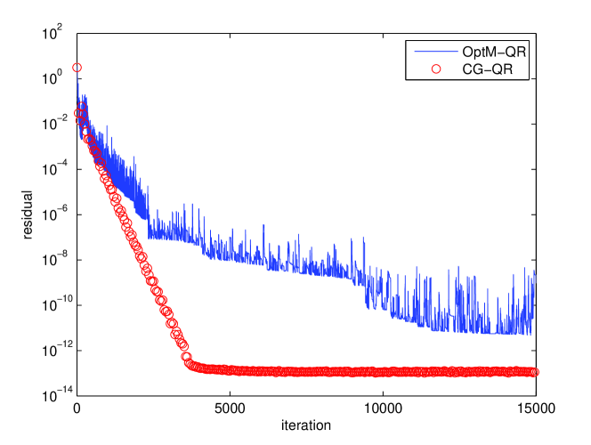
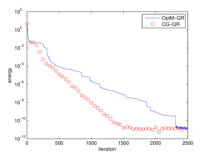
We then see the convergence curves for the residual ${|\kern-1.07639pt|\kern-1.07639pt|}\nabla_{G}E(U_{n}){|\kern-1.07639pt|\kern-1.07639pt|}$ and the error of the total energy. We take $C_{120}$ as an example. We understand from Table 1 that the numbers of iterations required for the convergence for the three conjugate gradient methods are almost the same, namely, they share the similar convergence curves. As a result, we only show the results obtained by CG-QR for illustration. The corresponding results are shown in Figure 1, where the x-axis is the number of iterations, the y-axis for the top part is the residual ${|\kern-1.07639pt|\kern-1.07639pt|}\nabla_{G}E(U_{n}){|\kern-1.07639pt|\kern-1.07639pt|}$, and the y-axis for the bottom part is the error of the energy $E(U_{n})-E_{min}$ ($E_{min}$ is a high-accuracy approximation of the exact total energy). We can see that the curves for both the residual and the error of the total energy obtained by Algorithm CG-QR are smoother than those obtained by Algorithm OptM-QR, which indicates that our algorithms are more stable than Algorithm OptM-QR. We understand that the oscillation of the ${|\kern-1.07639pt|\kern-1.07639pt|}\nabla_{G}E{|\kern-1.07639pt|\kern-1.07639pt|}$ curve for Algorithm OptM-QR is caused by the nonmonotonic behavior of the BB step size [6].

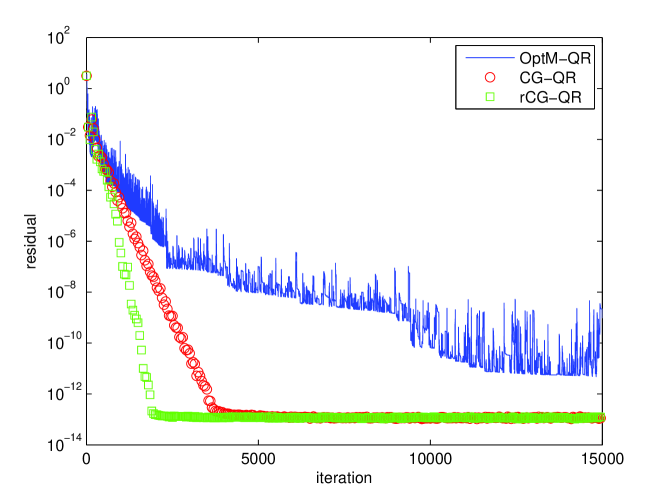
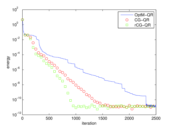
We now turn to illustrate the advantages of our Restarted Algorithms. We choose $g_{tol}=5.0\times 10^{-3}$ in our experiments. Other parameters are the same as those we chose in the previous experiments. We only focus on the algorithm rCG-QR since the QR strategy is better than others from our previous experiments. We observe that rCG-QR outperforms CG-QR much for alanine chain and $C_{120}$ for which plenty of iterations are required, while for other systems, rCG-QR performs similar with CG-QR. Therefore, we only show the detailed results for alanine chain and $C_{120}$ in Table 2. To see the behavior of OptM-QR, CG-QR and rCG-QR more clearly, we also take $C_{120}$ as an example and plot the convergence curves of the residual and the error of total energy for the three algorithms in Figure 2, from which we see that rCG-QR converges faster than CG-QR.

Table 2: The numerical results for alanine chain and $C_{120}$ obtained by different algorithms, $\theta=0.8$.

algorithm	energy (a.u.)	iter	${|\kern-0.96873pt|\kern-0.96873pt|}\nabla_{G}E{|\kern-0.96873pt|\kern-0.96873pt|}$	wall clock time (s)
alanine chain$(C_{33}H_{11}O_{11}N_{11})\ \ \ N_{g}=293725\ \ \ N=132\ \ \ cores=32$
OptM-QR	-4.78562217E+02	12276	9.93E-13	16028.13
CG-QR	-4.78562217E+02	2100	9.88E-13	1658.16
rCG-QR	-4.78562217E+02	1493	9.80E-13	1192.14
$C_{120}\ \ \ N_{g}=354093\ \ \ N=240\ \ \ cores=32$
OptM-QR	-6.84467048E+02	15000(fail)	9.70E-10	33184.12
CG-QR	-6.84467048E+02	3518	9.95E-13	5016.26
rCG-QR	-6.84467048E+02	1846	9.68E-13	2946.68

Fig. 2: Convergence curves for ${|\kern-1.07639pt|\kern-1.07639pt|}\nabla_{G}E{|\kern-1.07639pt|\kern-1.07639pt|}$ and the error of energy $E(U_{n})-E_{min}$ obtained by OptM-QR, CG-QR and rCG-QR for $C_{120}$.

7 Concluding remarks

We have proposed a conjugate gradient method for electronic structure calculations in this paper. Under some reasonable assumptions, we have proved the local convergence of our algorithms. It is shown by our numerical experiments that our algorithms are efficient. We believe these conjugate gradient algorithms can be further improved by using some preconditioners, which is indeed our on-going project. We should also point out that the choice in the Hessian based strategy may not be good when (38) fails, there should be a better strategy, which is also our on-going work.

Our algorithms can be naturally applied to extreme eigenvalue calculations for large scale symmetric matrices, where the smallest or largest $N$ eigenvalues and corresponding eigenvectors need to be computed. For matrix eigenvalue problems, Assumption 4 is always satisfied, and Assumption 5 is satisfied when there is a gap between the $N$-th and $(N+1)$-th eigenvalues [27], and thus our convergence result also holds. Our algorithms are simpler to implement than the projected preconditioned conjugate gradient algorithm proposed in [36], where several practical issues should be taken into account so as to achieve good performance and some choices of parameters are problems based.

In addition, our method can also be applied to other orthogonality constrained optimization problems which satisfy our assumptions, for instance, the low rank nearest correlation estimation [28], the quadratic assignment problem [3, 39], etc. For these nonlinear problems where the calculations of Hessian are not easy, some quasi-Newton method may be used to update the Hessian. Anyway, our method should be a quite general approach for optimization problems with orthogonality constraint.

Finally, we should mention that the algorithm OptM-QR proposed in [42] needs less memories at each iteration since it is a gradient type method with BB step sizes. Besides, although the conjugate gradient method is superior in terms of asymptotic performance, the BB method gives reasonable results for relatively high tolerances, which makes the BB method useful in some applications. We also understand from [9] that the BB method may outperform the conjugate gradient method in some other cases.

Appendix A A Proof of Lemma 6

To prove Lemma 6, we first introduce some notation and a lemma. For a diagonal matrix $\mathcal{D}=\text{diag}(d_{1},d_{2},\cdots,d_{N})$, we use $\sin{\mathcal{D}}$ to denote $\text{diag}(\sin{d_{1}},\sin{d_{2}},\cdots,\sin{d_{N}})$, with similar notation for $\cos{\mathcal{D}}$, $\arcsin{\mathcal{D}}$ and $\arccos{\mathcal{D}}$.

Lemma 18.

For $\Psi=(\psi_{1},\cdots,\psi_{N})\in\mathcal{M}_{N_{g}}^{N}$ and $\Phi=(\phi_{1},\cdots,\phi_{N})\in\mathcal{M}_{N_{g}}^{N}$, $[\Psi]\neq[\Phi]$, there exists a curve $\Gamma(t)\in\mathcal{M}_{N_{g}}^{N},\ t\in[0,1]$, such that $[\Gamma(0)]=[\Psi]$, $[\Gamma(1)]=[\Phi]$, $\textup{dist}([\Gamma(t)],[\Psi])\leq\textup{dist}([\Phi],[\Psi])$, and

(78) $$\Gamma(t)^{T}\Gamma^{\prime}(t)=0.$$

Proof.

Let $\Psi^{T}\Phi=ASB^{T}$ be the SVD of $\Psi^{T}\Phi$. We obtain from $\Psi\in\mathcal{M}_{N_{g}}^{N}$ and $\Phi\in\mathcal{M}_{N_{g}}^{N}$ that $S=\text{diag}(s_{1},s_{2},\cdots,s_{N})$ is a diagonal matrix with $s_{i}\in[0,1]$, and hence we denote the diagonal matrix $\arccos S$ by $\Theta$, which means that $\Theta=\text{diag}(\theta_{1},\theta_{2},\cdots,\theta_{N})$ with $\theta_{i}=\arccos s_{i}$. Let $A_{2}S_{2}B_{2}^{T}$ be the SVD of $\Phi-\Psi(\Psi^{T}\Phi)$, where $A_{2}\in\mathcal{M}_{N_{g}}^{N}$, $S_{2}$ is a diagonal matrix containing the singular values, and $B_{2}\in\mathcal{O}^{N\times N}$. Then there holds

$$B_{2}S_{2}^{2}B_{2}^{T} = (\Phi-\Psi(\Psi^{T}\Phi))^{T}(\Phi-\Psi(\Psi^{T}\Phi))$$

$$= I_{N}-(\Psi^{T}\Phi)^{T}(\Psi^{T}\Phi)=I_{N}-BS^{2}B^{T}=B(\sin\Theta)^{2}B^{T}.$$

As a result, we may choose $S_{2}=\sin\Theta$, $B_{2}=B$, and obtain $\Phi-\Psi(\Psi^{T}\Phi)=A_{2}\sin\Theta B^{T}$. Let

(79) $$\Gamma(t)=\Psi A\cos\Theta t+A_{2}\sin\Theta t.$$

It is easy to verify that $\Gamma(t)\in\mathcal{M}_{N_{g}}^{N}$, $[\Gamma(0)]=[\Psi]$, $[\Gamma(1)]=[\Phi]$, and $\Gamma(t)^{T}\Gamma^{\prime}(t)=0$. Furthermore,

$${|\kern-1.07639pt|\kern-1.07639pt|}\Gamma(t)-\Psi A{|\kern-1.07639pt|\kern-1.07639pt|}^{2} = {|\kern-1.07639pt|\kern-1.07639pt|}\Psi A(\cos\Theta t-I_{N})+A_{2}\sin\Theta t{|\kern-1.07639pt|\kern-1.07639pt|}^{2}$$

$$= \text{tr}((\cos\Theta t-I_{N})^{2}+(\sin\Theta t)^{2})$$

$$= \text{tr}(2I_{N}-2\cos\Theta t).$$

We understand from $s_{i}\in[0,1]$ that $\theta_{i}\in[0,\frac{\pi}{2}]$, which implies that ${|\kern-1.07639pt|\kern-1.07639pt|}\Gamma(t)-\Psi A{|\kern-1.07639pt|\kern-1.07639pt|}^{2}$ is monotonically non-decreasing for $t\in[0,1]$. We then get from the proof of Lemma 3 that

$${|\kern-1.07639pt|\kern-1.07639pt|}\Gamma(t)-\Psi A{|\kern-1.07639pt|\kern-1.07639pt|}^{2}\leq{|\kern-1.07639pt|\kern-1.07639pt|}\Gamma(1)-\Psi A{|\kern-1.07639pt|\kern-1.07639pt|}^{2}=\text{tr}(2I_{N}-2\cos\Theta)=\text{dist}([\Phi],[\Psi]).$$

Hence we have $\text{dist}([\Gamma(t)],[\Psi])\leq\text{dist}([\Phi],[\Psi])$. This completes the proof. ∎

We should point out that our proof here is inspired by the geodesic formula on page 11 of [1], where the invertibility of $\Psi^{T}\Phi$ is required. However, we do not need this condition to get $\Gamma(t)$.

Now we turn to prove Lemma 6.

Proof of Lemma 6:

Proof.

Let us prove the first conclusion by contradiction. Assume that there exists $[V^{*}]\in B([U^{*}],\delta_{1})$, $[V^{*}]\neq[U^{*}]$, such that $\nabla_{G}E(V^{*})=0$. We see from Assumption 5 that $[V^{*}]$ is also a local minimizer of the energy functional. We obtain from Lemma 18 that there exists a curve $\Gamma(t)\in\mathcal{M}_{N_{g}}^{N},\ t\in[0,1]$, such that $[\Gamma(0)]=[U^{*}]$, $[\Gamma(1)]=[V^{*}]$, $[\Gamma(t)]\in B([U^{*}],\delta_{1})$, and

$$(\Gamma(t))^{T}\Gamma^{\prime}(t)=0,$$

which implies that $\Gamma^{\prime}(t)$ is in the tangent space of $\Gamma(t)$ on the Grassmann manifold. Since $E(\Gamma(t))$ is continuous in $[0,1]$, and $[U^{*}]$, $[V^{*}]$ are local minimizers, we have that there is a $t_{0}\in(0,1)$, such that $\Gamma(t_{0})$ is the maximizer of $E(\Gamma(t)),\ t\in[0,1]$. This indicates that

$$\text{tr}(\nabla_{G}E(\Gamma(t_{0}))^{T}\Gamma^{\prime}(t_{0}))=0.$$

Further, since $\Gamma(t_{0})$ is the maximizer of $E(\Gamma(t))$ on this curve, we see that

$$\text{Hess}_{G}E(\Gamma(t_{0}))[\Gamma^{\prime}(t_{0}),\Gamma^{\prime}(t_{0})]\leq 0,$$

which contradicts with the coercivity assumption in Assumptions 5. Namely, there exists only one stationary point $[U^{*}]$ in $B([U^{*}],\delta_{1})$ on the Grassmann manifold.

Now we prove the second conclusion by contradiction too. If (23) is not true, then there exists $\hat{\delta}>0$ and a subsequence $\{V_{n_{k}}\}_{k=1}^{\infty}$ of $\{V_{n}\}_{n=1}^{\infty}$, such that

$$\text{dist}([V_{n_{k}}],[U^{*}])\geq\hat{\delta},\ \forall\ k\geq 0.$$

We obtain from Lemma 3 that for each $k$, there exists $P_{n_{k}}\in\mathcal{O}^{N\times N}$ satisfying

$${|\kern-1.07639pt|\kern-1.07639pt|}V_{n_{k}}P_{n_{k}}-U^{*}{|\kern-1.07639pt|\kern-1.07639pt|}=\text{dist}([V_{n_{k}}],[U^{*}])\geq\hat{\delta}.$$

Since $\{V_{n_{k}}P_{n_{k}}\}_{k=1}^{\infty}$ are bounded and $\mathcal{M}^{N}_{N_{g}}$ is compact, we get that there exists a subsequence $\{V_{n_{k_{j}}}P_{n_{k_{j}}}\}_{j=1}^{\infty}$ and $U_{0}$, such that $\lim\limits_{j\to\infty}{|\kern-1.07639pt|\kern-1.07639pt|}V_{n_{k_{j}}}P_{n_{k_{j}}}-U_{0}{|\kern-1.07639pt|\kern-1.07639pt|}=0$. Then, we obtain from $\lim\limits_{n\to\infty}E(V_{n})=E(U^{*})$ that

(80) $$E(U_{0})=\lim_{j\to\infty}E(V_{n_{k_{j}}}P_{n_{k_{j}}})=\lim_{j\to\infty}E(V_{n_{k_{j}}})=E(U^{*}).$$

Due to $[V_{n_{k_{j}}}P_{n_{k_{j}}}]\in B([U^{*}],\delta_{1})$, we have that $[U_{0}]\in B([U^{*}],\delta_{1})$, which together with (80) yields that $[U_{0}]$ is also a minimizer of the energy functional in $B([U^{*}],\delta_{1})$. Therefore, we obtain $\nabla_{G}E(U_{0})=0$. We conclude from the proof for the first conclusion that $[U_{0}]=[U^{*}]$, which contradicts with $\text{dist}([V_{n_{k_{j}}}],[U^{*}])\geq\hat{\delta}$. This completes the proof. ∎

Appendix B B Numerical tests of the step sizes

In this appendix, we will report some more numerical results for the algorithms using different step sizes and different calculation formulas for the Hessian, which lead to our recommendation. The detailed results are listed in Table 3.

First, we introduce some notation used in Table 3.

• OptM-QR-BB: the OptM-QR method with BB step size proposed in [42];

• OptM-QR-aH: OptM-QR with the Hessian based step size (39), where $D_{n}$ is replaced by $\nabla_{G}E(U_{n})$ and the approximate Hessian (17) is used;

• OptM-QR-H: OptM-QR with the Hessian based step size (39), where $D_{n}$ is replaced by $\nabla_{G}E(U_{n})$, and the exact Hessian (16) is used;

• CG-QR-BB: the CG-QR algorithm with BB step size;

• CG-QR-aH: the CG-QR algorithm with the Hessian based step size (39) and the approximate Hessian (17) being used;

• CG-QR-H: the CG-QR algorithm with the Hessian based step size (39) and the exact Hessian (16) being used.

We should point out that CG-QR-aH here is just CG-QR in the former part of this paper, and OptM-QR-BB here is just OptM-QR in the former part of this paper.

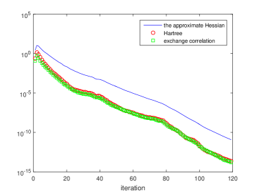
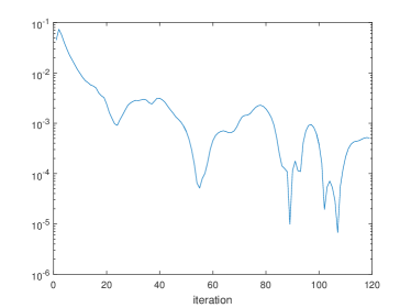
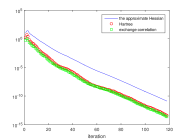
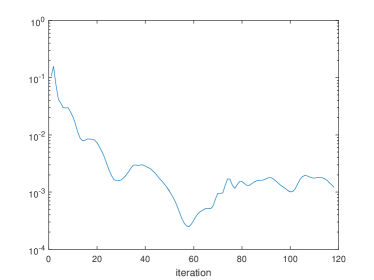
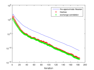
We first take a look at the results obtained by our CG algorithms using the approximate Hessian (17) and the exact Hessian (16), respectively. By the comparison, we can see that the algorithms using the exact Hessian (16) require as much iterations as the algorithms using the approximate Hessian (17), while the former spends of course more time than the latter one. To understand this numerical phenomenon, we show the changes of the approximate Hessian (17), the Hartree term (second line of (16)) and the exchange and correlation term (third line of (16)) as a function of the number of iteration in Figure 3. We can see that in most cases, the last two terms are much smaller than the approximate Hessian term, which means that they contribute little to the exact Hessian and can be neglected. Therefore, taking the cost and the accuracy into account, we recommend to use the approximate Hessian (17) instead of the exact Hessian (16).

We then compare the efficiency of algorithms with different step sizes. We observe from Table 3 that when using the Hessian-based step size, CG algorithms outperform OptM-QR much. Furthermore, based on our numerical experiments, we should point out that the BB step size is almost the most suitable one for the gradient method while it may not be so good for the CG methods.

Table 3: Numerical results for systems with different sizes obtained by different algorithms.

algorithm	energy (a.u.)	iter	${|\kern-0.96873pt|\kern-0.96873pt|}\nabla_{G}E{|\kern-0.96873pt|\kern-0.96873pt|}$	wall clock time (s)
benzene($C_{6}H_{6})\ \ \ N_{g}=102705\ \ \ N=15\ \ \ cores=8$
OptM-QR-BB	-3.74246025E+01	164	7.49E-07	6.63
OptM-QR-aH	-3.74246025E+01	1753	9.92E-07	67.83
OptM-QR-H	-3.74246025E+01	1771	9.92E-07	86.33
CG-QR-BB	-3.74246025E+01	249	9.98E-07	10.41
CG-QR-aH	-3.74246025E+01	118	9.94E-07	5.56
CG-QR-H	-3.74246025E+01	119	9.10E-07	7.26
aspirin($C_{9}H_{8}O_{4})\ \ \ N_{g}=133828\ \ \ N=34\ \ \ cores=16$
OptM-QR-BB	-1.20214764E+02	153	9.89E-07	14.63
OptM-QR-aH	-1.20214764E+02	1271	9.92E-07	137.97
OptM-QR-H	-1.20214764E+02	1275	9.89E-07	165.61
CG-QR-BB	-1.20214764E+02	220	7.94E-07	25.28
CG-QR-aH	-1.20214764E+02	118	9.68E-07	15.15
CG-QR-H	-1.20214764E+02	118	9.50E-07	17.94
$C_{60}\ \ \ N_{g}=191805\ \ \ N=120\ \ \ cores=16$
OptM-QR-BB	-3.42875137E+02	234	7.17E-07	92.17
OptM-QR-aH	-3.42875137E+02	3155	9.90E-07	1617.35
OptM-QR-H	-3.42875137E+02	3096	9.97E-07	1642.80
CG-QR-BB	-3.42875137E+02	332	9.20E-07	152.85
CG-QR-aH	-3.42875137E+02	184	9.78E-07	98.64
CG-QR-H	-3.42875137E+02	184	9.74E-07	104.29
alanine chain$(C_{33}H_{11}O_{11}N_{11})\ \ \ N_{g}=293725\ \ \ N=132\ \ \ cores=32$
OptM-QR-BB	-4.78562217E+02	1558	9.49E-07	906.95
OptM-QR-aH	-4.78562217E+02	30000	4.42E-06	23404.10
OptM-QR-H	-4.78562216E+02	30000	7.54E-05	29684.30
CG-QR-BB	-4.78562217E+02	3190	9.59E-07	2338.59
CG-QR-aH	-4.78562217E+02	1017	9.93E-07	818.32
CG-QR-H	-4.78562217E+02	1232	1.00E-06	1204.82
$C_{120}\ \ \ N_{g}=354093\ \ \ N=240\ \ \ cores=32$
OptM-QR-BB	-6.84467048E+02	2024	9.53E-07	2119.55
OptM-QR-aH	-6.84467047E+02	30000	5.67E-05	41941.88
OptM-QR-H	-6.84467046E+02	30000	5.74E-05	44111.19
CG-QR-BB	-6.84467048E+02	3573	9.88E-07	4426.20
CG-QR-aH	-6.84467048E+02	1490	9.93E-07	2164.48
CG-QR-H	-6.84467048E+02	1324	9.89E-07	2019.65
$C_{1015}H_{460}\ \ \ N_{g}=1462257\ \ \ N=2260\ \ \ cores=256$
OptM-QR-BB	-6.06369982E+03	137	3.38E-05	4813.73
OptM-QR-aH	-6.06369982E+03	1078	7.57E-05	43975.26
OptM-QR-H	-6.06369982E+03	1102	7.58E-05	45701.15
CG-QR-BB	-6.06369982E+03	163	6.36E-05	7511.18
CG-QR-aH	-6.06369982E+03	104	7.03E-05	4640.49
CG-QR-H	-6.06369982E+03	104	7.05E-05	4724.56
$C_{1419}H_{556}\ \ \ N_{g}=1828847\ \ \ N=3116\ \ \ cores=512$
OptM-QR-BB	-8.43085432E+03	151	1.01E-04	7769.35
OptM-QR-aH	-8.43085432E+03	988	1.01E-04	56845.33
OptM-QR-H	-8.43085432E+03	1054	9.99E-05	61326.61
CG-QR-BB	-8.43085432E+03	200	9.16E-05	13495.65
CG-QR-aH	-8.43085432E+03	103	1.00E-04	5568.38
CG-QR-H	-8.43085432E+03	103	1.00E-04	6578.48

Fig. 3: Left: changes of each term in Hessian $\textup{Hess}_{G}E(U_{n})[D_{n},D_{n}]$ with iteration. Right: the quotient of the sum of the Hartree and exchange correlation terms divided by the approximate Hessian. (for algorithm CG-QR-H).

benzene

aspirin

$C_{60}$

alanine chain

$C_{120}$

$C_{1015}H_{460}$

$C_{1419}H_{556}$

References

- [1] P.-A. Absil, R. Mahony, and R. Sepulchre, Riemannian geometry of Grassmann manifolds with a view on algorithmic computation, Acta Appl. Math. 80 (2), (2004), pp. 199-220.
- [2] P.-A. Absil, R. Mahony, and R. Sepulchre, Optimization Algorithms on Matrix Manifolds, Princeton University Press, Princeton, 2008.
- [3] R. E. Burkard, S. E. Karisch, and F. Rendl, QAPLIB-a quadratic assignment problem library, J. Global Optim., 10 (1997), pp. 391-403.
- [4] X. Dai, X. Gong, A. Zhou, and J. Zhu, A parallel orbital-updating approach for electronic structure calculations, arXiv:1405.0260 (2014).
- [5] X. Dai and A. Zhou, Finite element methods for electronic structure calculations, Sci. Sin. Chem., 45 (2015), pp. 800-811 (in Chinese).
- [6] Y. Dai, Alternate step gradient method, Optimization, 52 (2003), pp. 395-415.
- [7] Y. Dai and Y. Yuan, A nonlinear conjugate gradient method with a strong global convergence property, SIAM J. Optim., 10 (1999), pp. 177-182.
- [8] A. Edelman, T. A. Arias, and S. T. Smith, The geometry of algorithms with orthogonality constraints, SIAM J. Matrix Anal. Appl., 20 (1998), pp. 303-353.
- [9] R. Flecher, On the Barzilai-Borwein method, in Optimization and Control with Applications, Appl. Optim. 96, Springer, New York, 2005, pp. 235-256.
- [10] S. Fournais, M. Hoffmann-Ostenhof, T. Hoffmann-Ostenhof AND T. . Srensen, Positivity of the spherically averaged atomic one-electron density, Math. Z., 259(2008), pp. 123-130.
- [11] J. B. Francisco, J. M. Martinez, and L. Martinez, Globally convergent trust-region methods for self-consistent field electronic structure calculations, J. Chem. Phys., 121 (2004), pp. 10863-10878.
- [12] B. Gao, X. Liu, X. Chen, and Y. Yuan, A new first-order framework for orthogonal constrained optimization problems, \urlhttp://www.optimization-online.org/DB_HTML/2016/09/5660.html, 2016.
- [13] G. H. Golub, and C. F. Van Loan, Matrix Computations, The Johns Hopkins University Press, Baltimore, 2013, pp. 75-77.
- [14] W.W. Hager, H. Zhang, A Survey of nonlinear conjugate gradient methods, \urlhttp://people.cs.vt.edu/ asandu/Public/Qual2011/Optim/Hager_2006_CG-survey.pdf, 2006.
- [15] P. Hohenberg and W. Kohn, Inhomogeneous electron gas, Phys. Rev. B., 136 (1964), pp. 864-871.
- [16] R. A. Horn and C. R. Johnson, Matrix Analysis, Cambridge University Press, 2012.
- [17] B. Jiang and Y. Dai, A framework of constraint preserving update schemes for optimization on Stiefel manifold, Math. Program., 153 (2015), pp. 535-575.
- [18] W. Kohn and L. J. Sham, Self-consistent equations including exchange and correlation effects, Phys. Rev. A., 140 (1965), pp. 4743-4754.
- [19] X. Liu, Z. Wen, X. Wang, M. Ulbrich, and Y. Yuan, On the analysis of the discretized Kohn-Sham density functional theory, SIAM J. Numer. Anal., 53 (2015), pp. 1758-1785.
- [20] X. Liu, X. Wang, Z. Wen, and Y. Yuan, On the convergence of the self-consistent field iteration in Kohn-Sham density functional theory, SIAM J. Matrix Anal. Appl., 35 (2014), pp. 546-558.
- [21] R. Martin, Electronic Structure: Basic Theory and Practical Methods, Cambridge university Press, London, 2004.
- [22] R. G. Parr and W. T. Yang, Density-Functional Theory of Atoms and Molecules, Clarendon Press, Oxford, 1994.
- [23] M.C. Payne, M. P. Teter, D.C. Allan, and J.D. Joannopoulos, Iterative minimization techniques for ab initio total-energy calculations: molecular dynamics and conjugate gradients, Rev. Modern Phys., 64 (1992), pp. 1045-1097.
- [24] J. P. Perdew and A. Zunger, Self-interaction correction to density functional approximations for many-electron systems, Phys. Rev. B., 23 (1981), pp. 5048-5079.
- [25] M. J. D. Powell, Restart procedures of the conjugate gradient method, Math. Prog., 2 (1977), pp. 241-254.
- [26] Y. Saad, J. R. Chelikowsky, and S. M. Shontz, Numerical methods for electronic structure calculations of materials, SIAM Review, 52(1) (2010), pp. 3-54.
- [27] R. Schneider, T. Rohwedder, A. Neelov, and J. Blauert, Direct minimization for calculating invariant subspaces in density fuctional computations of the electronic structure, J. Comput. Math., 27 (2009), pp. 360-387.
- [28] D. Simon and J. Abell, A majorization algorithm for constrained correlation matrix approximation, Linear Algebra Appl., 432 (2010), pp. 1152-1164.
- [29] S. T. Smith, Geometric Optimization Methods for Adaptive Filtering, PhD thesis, Harvard University, Cambridge, MA, 1993.
- [30] S. T. Smith, Optimization techniques on Riemannian manifolds, in Fields Institute Communications, Vol. 3, AMS, Providence, RI, 1994, pp. 113-146.
- [31] I. Štich, R. Car, M. Parrinello, and S. Baroni, Conjugate gradient minimization of the energy functional: A new method for electronic structure calculation, Phys. Rev. B, 39 (1989), pp. 4997-5004.
- [32] N. Troullier and J. L. Martins, Efficient pseudopotentials for plane-wave calculations, Phys. Rev. B., 43 (1991), pp. 1993-2006.
- [33] M.P. Teter, M.C. Payne, and D.C. Allan, Solution of Schrödinger’s equation for large systems, Phys. Rev. B, 40 (1989), pp. 12255-12263.
- [34] L. Thøgersen, J. Olsen, D. Yeager, P. Jørgensen, P. Sałek, and T. Helgaker, The trustregion self-consistent field method: Towards a black-box optimization in Hartree-Fock and Kohn-Sham theories, J. Chem. Phys., 121 (2004), pp. 16-27.
- [35] M. Ulbrich, Z. Wen, C. Yang, D. Klöckner, and Z. Lu, A proximal gradient method for ensemble density functional theory, SIAM J. Sci. Comput., 37 (2015), pp. A1975-A2002.
- [36] E. Vecharynski, C. Yang, and J. E. Pask, A projected preconditioned conjugate gradient algorithm for computing a large invariant subspace of a Hermitian matrix, J. Comput. Phys., 290 (2015), pp. 73-89.
- [37] Z. Wen, A. Milzarek, M. Ulbrich, and H. Zhang, Adaptive regularized self-consistent field iteration with exact Hessian for electronic structure calculation, SIAM J. Sci. Comput., 35 (2013), pp. A1299-A1324.
- [38] Z. Wen, C. Yang, X. Liu, and Y. Zhang, Trace penalty minimization for large-scale eigenspace computation, J. Sci. Comput., 66 (2016), pp. 1175-1203.
- [39] Z. Wen and W. Yin, A feasible method for optimization with orthogonality constraints, Math. Program. Ser. A., 142 (2013), pp. 397-434.
- [40] C. Yang, W. Gao, and J. Meza, On the convergence of the self-consistent field iteration for a class of nonlinear eigenvalue problems, SIAM J. Matrix Anal. Appl., 30 (2009), pp. 1773-1788.
- [41] C. Yang, J. C. Meza, and L. Wang, A trust region direct constrained minimization algorithm for the Kohn-Sham equation, SIAM J. Sci. Comput., 29 (2007), pp. 1854-1875.
- [42] X. Zhang, J. Zhu, Z. Wen and A. Zhou, Gradient type optimization methods for electronic structure calculations, SIAM J. Sci. Comput., 36 (2014), pp. 265-289.