Non-Gaussian Component Analysis
with Log-Density Gradient Estimation

Abstract

Non-Gaussian component analysis (NGCA) is aimed at identifying a linear subspace such that the projected data follows a non-Gaussian distribution. In this paper, we propose a novel NGCA algorithm based on log-density gradient estimation. Unlike existing methods, the proposed NGCA algorithm identifies the linear subspace by using the eigenvalue decomposition without any iterative procedures, and thus is computationally reasonable. Furthermore, through theoretical analysis, we prove that the identified subspace converges to the true subspace at the optimal parametric rate. Finally, the practical performance of the proposed algorithm is demonstrated on both artificial and benchmark datasets.

1 Introduction

A popular way to alleviate difficulties of handling high-dimensional data is to reduce the dimensionality of data. Real-world applications imply that a small number of non-Gaussian signal components in data often include “interesting” information, while the remaining Gaussian components are “uninteresting” (Blanchard et al., 2006). This is the fundamental motivation of non-Gaussian-based unsupervised dimension reduction methods.

A well-known method is projection pursuit (PP), which estimates directions on which the projected data is as non-Gaussian as possible (Friedman and Tukey, 1974; Huber, 1985). In practice, PP algorithms maximize a single index function measuring non-Gaussianity of the data projected on a direction. However, some index functions are suitable for measuring super-Gaussianity, while others are good at measuring sub-Gaussianity (Hyvärinen et al., 2001). Thus, PP algorithms might not work well when super- and sub-Gaussian signal components are mixtured in data.

Non-Gaussian component analysis (NGCA) (Blanchard et al., 2006) copes with this problem. NGCA is a semi-parametric framework for unsupervised linear dimension reduction, and aimed at identifying a subspace such that the projected data follows a non-Gaussian distribution. Compared with independent component analysis (ICA) (Comon, 1994; Hyvärinen et al., 2001), NGCA stands on a more general setting: There is no restriction about the number of Gaussian components and non-Gaussian signal components can be dependent of each other, while ICA makes a stronger assumption that at most one Gaussian component is allowed and all the signal components are statistically independent of each other.

To take into account both super- and sub-Gaussian components, the first practical NGCA algorithm called the multi-index projection pursuit (MIPP) heuristically makes use of multiple index functions in PP (Blanchard et al., 2006), but it seems to be unclear whether this heuristic works well in general. To improve the performance of MIPP, iterative metric adaptation for radial kernel functions (IMAK) has been proposed (Kawanabe et al., 2007). IMAK does not rely on index functions, but instead estimates alternative functions from data. However, IMAK involves an iterative optimization procedure, and its computational cost is expensive.

In this paper, based on log-density gradient estimation, we propose a novel NGCA algorithm which we call the least-squares NGCA (LSNGCA). The rationale in LSNGCA is that as we show later, the target subspace contains the log-gradient for the data density subtracted by the log-gradient for a Gaussian density. Thus, the subspace can be identified using the eigenvalue decomposition. Unlike MIPP and IMAK, LSNGCA neither requires index functions nor any iterative procedures, and thus is computationally reasonable.

A technical challenge in LSNGCA is to accurately estimate the gradient of the log-density for data. To overcome it, we employ a direct estimator called the least squares log-density gradients (LSLDG) (Cox, 1985; Sasaki et al., 2014). LSLDG accurately and efficiently estimates log-density gradients in a closed form without going through density estimation. In addition, it includes an automatic parameter tuning method. In this paper, based on LSLDG, we theoretically prove that the subspace identified by LSNGCA converges to the true subspace at the optimal parametric rate, and finally demonstrate that LSNGCA reasonably works well on both artificial and benchmark datasets.

This paper is organized as follows: In Section 2, after stating the problem of NGCA, we review MIPP and IMAK, and discuss their drawbacks. We propose LSNGCA, and then overview LSLDG in Section 3. Section 4 performs a theoretical analysis of LSNGCA. The performance of LSNGCA on artificial datasets is illustrated in Sections 5. Application to binary classification on benchmark datasets is given in Section 6. Section 7 concludes this paper.

2 Review of Existing Algorithms

In this section, we first describe the problem of NGCA, and then review existing NGCA algorithms.

2.1 Problem Setting

Suppose that a number of samples $\mathcal{X}=\{\bm{x}_{i}=(x_{i}^{(1)},x_{i}^{(2)},\dots,x_{i}^{(d_{\bm{\mathrm{x}}})})^{\top}\}_{i=1}^{n}$ are generated according to the following model:

$$\bm{x}=\mathbf{A}\bm{s}+\bm{n},$$ (1)

where $\bm{s}=(s^{(1)},s^{(2)},\dots,s^{(d_{\bm{\mathrm{s}}})})^{\top}$ denotes a random signal vector, $\mathbf{A}$ is a $d_{\bm{\mathrm{x}}}$-by-$d_{\bm{\mathrm{s}}}$ matrix, $\bm{n}$ is a Gaussian noise vector with the mean vector $\bm{0}$ and covariance matrix $\mathbf{C}$. Assume further that the dimensionality of $\bm{s}$ is lower than that of $\bm{x}$, namely $d_{\bm{\mathrm{s}}}<d_{\bm{\mathrm{x}}}$, and $\bm{s}$ and $\bm{n}$ are statistically independent of each other.

Lemma 1 in Blanchard et al. (2006) states that when data samples follow the generative model (1), the probability density $p(\bm{x})$ can be described as a semi-parametric model:

$$p(\bm{x})=f_{\bm{\mathrm{x}}}(\mathbf{B}^{\top}\bm{x})\phi_{\mathbf{C}}(\bm{x}),$$ (2)

where $\mathbf{B}$ is a $d_{\bm{\mathrm{x}}}$-by-$d_{\bm{\mathrm{s}}}$ matrix, $f_{\bm{\mathrm{x}}}$ is a positive function and $\phi_{\mathbf{C}}$ denotes the Gaussian density with the mean $\bm{0}$ and covariance matrix $\mathbf{C}$.

The decomposition in (2) is not unique because $f_{\bm{\mathrm{x}}}$, $\mathbf{B}$ and $\mathbf{C}$ are not identifiable from $p$. However, as shown in Theis and Kawanabe (2006), the following linear $d_{\bm{\mathrm{s}}}$-dimensional subspace is identifiable:

$$\mathcal{L}=\text{Ker}(\mathbf{B}^{\top})^{\perp}=\text{Range}(\mathbf{B}).$$ (3)

$\mathcal{L}$ is called the non-Gaussian index space. Here, the problem is to identify $\mathcal{L}$ from $\mathcal{X}$. In this paper, we assume that $d_{\bm{\mathrm{s}}}$ is known.

2.2 Multi-Index Projection Pursuit

The first algorithm of NGCA called the multi-index projection pursuit (MIPP) was proposed based on the following key result (Blanchard et al., 2006):

Proposition 1.

Let $\bm{x}$ be a random variable whose density $p(\bm{x})$ has the semi-parametric form (2), and suppose that $h(\bm{x})$ is a smooth real function on $\mathbb{R}^{d_{\bm{\mathrm{x}}}}$. Denoting by $\mathbf{I}_{d_{\bm{\mathrm{x}}}}$ the $d_{\bm{\mathrm{x}}}$-by-$d_{\bm{\mathrm{x}}}$ identity matrix, assume further that $E\{\bm{x}\}=\bm{0}$ and $E\{\bm{x}\bm{x}^{\top}\}=\mathbf{I}_{d_{\bm{\mathrm{x}}}}$. Then, under mild regularity conditions on $h$, the following $\bm{\beta}(h)$ belongs to the target space $\mathcal{L}$:

$$\bm{\beta}(h)=E\{\bm{x}h(\bm{x})-\nabla_{\bm{x}}h(\bm{x})\},$$

where $\nabla_{\bm{x}}$ is the differential operator with respect to $\bm{x}$.

The condition that $E\{\bm{x}\bm{x}^{\top}\}=\mathbf{I}_{d_{\bm{\mathrm{x}}}}$ seems to be strong, but in practice it can be satisfied by whitening data. Based on Proposition 1, after whitening data samples as $\bm{y}_{i}=\widehat{\mathbf{\Sigma}}^{-1/2}\bm{x}_{i}$ where $\widehat{\mathbf{\Sigma}}=\frac{1}{n}\sum_{i=1}^{n}\bm{x}_{i}\bm{x}_{i}^{\top}$, for a bunch of functions $\left\{h_{k}\right\}_{k=1}^{K}$, MIPP estimates $\bm{\beta}(h_{k})=\bm{\beta}_{k}$ as

$$\widehat{\bm{\beta}}_{k}=\frac{1}{n}\sum_{i=1}^{n}\bm{y}_{i}h_{k}(\bm{y}_{i})-\nabla_{\bm{y}}h_{k}(\bm{y}_{i}).$$ (4)

Then, MIPP applies PCA to $\{\widehat{\bm{\beta}}_{k}\}_{k=1}^{K}$ and estimates $\mathcal{L}$ by pulling back the $d_{\bm{\mathrm{s}}}$-dimensional space spanned by the first $d_{\bm{\mathrm{s}}}$ principal directions into the original (non-whitened) space.

Although the basic procedure of MIPP is simple, there are two implementation issues: normalization of $\widehat{\bm{\beta}}_{k}$ and choice of functions $h_{k}$. The normalization issue comes from the fact that since (4) is a linear mapping, $\widehat{\bm{\beta}}_{k}$ with larger norm can be dominant in the PCA step, and they are not necessarily informative in practice. To cope with this problem, Blanchard et al. (2006) proposed the following normalization scheme:

$$\frac{\widehat{\bm{\beta}}_{k}}{\sqrt{\sum_{i=1}^{n}\|\bm{y}_{i}h_{k}(\bm{y}_{i})-\nabla_{\bm{y}}h_{k}(\bm{y}_{i})\|^{2}-\|\widehat{\bm{\beta}}_{k}\|^{2}}}.$$ (5)

After normalization, since the squared norm of each vector is proportional to its signal-to-noise ratio, longer vectors are more informative.

MIPP is supported by theoretical analysis (Blanchard et al., 2006, Theorem 3), but the practical performance strongly depends on the choice of $h$. To find an informative $h$, the form of $h$ was restricted as

$$h_{f,\bm{\omega}}(\bm{y})=r(\bm{\omega}^{\top}\bm{y}),$$

where $\bm{\omega}\in\mathbb{R}^{d_{\bm{\mathrm{x}}}}$ denotes a unit-norm vector, and $r$ is a function. As a heuristic, the FastICA algorithm (Hyvärinen, 1999) was employed to find a good $\bm{\omega}$. Although MIPP was numerically demonstrated to outperform PP algorithms, it is unclear whether these heuristic restriction and preprocessing work well in general.

2.3 Iterative Metric Adaptation for Radial Kernel Functions

To improve the performance of MIPP, the iterative metric adaptation for radial kernel functions (IMAK) estimates $h$ by directly maximizing the informative normalization criterion, which is the squared norm of (5) used for normalization in MIPP (Kawanabe et al., 2007). To estimate $h$, a linear-in-parameter model is used as

$$h_{\sigma^{2},\mathbf{M},\bm{\alpha}}(\bm{y}) =\sum_{i=1}^{n}\alpha_{i}\exp\left\{-\frac{1}{2\sigma^{2}}(\bm{y}-\bm{y}_{i})^{\top}\mathbf{M}(\bm{y}-\bm{y}_{i})\right\}$$

$$=\sum_{i=1}^{n}\alpha_{i}k_{\sigma^{2},\mathbf{M}}(\bm{y},\bm{y}_{i}),$$

where $\bm{\alpha}=(\alpha_{1},\dots,\alpha_{n})$ is a vector of parameters to be estimated, $\mathbf{M}$ is a positive semidefinite matrix and $\sigma$ is a fixed scale parameter. This model allows us to represent the squared norm of the informative criterion (5) as

$$\frac{\|\widehat{\bm{\beta}}_{k}\|^{2}}{\sum_{i=1}^{n}\|\bm{y}_{i}h_{k}(\bm{y}_{i})-\nabla_{\bm{y}}h_{k}(\bm{y}_{i})\|^{2}-\|\widehat{\bm{\beta}}_{k}\|^{2}}=\frac{\bm{\alpha}^{\top}\mathbf{F}\bm{\alpha}}{\bm{\alpha}^{\top}\mathbf{G}\bm{\alpha}}.$$ (6)

$\mathbf{F}$ and $\mathbf{G}$ in (6) are given by

$$a \mathbf{F}=\frac{1}{n^{2}}\sum_{r=1}^{d_{\bm{\mathrm{x}}}}\left(\bm{e}_{r}^{\top}\mathbf{Y}\mathbf{K}-\bm{1}_{n}^{\top}\partial_{r}\mathbf{K}\right)^{\top}\left(\bm{e}_{r}^{\top}\mathbf{Y}\mathbf{K}-\bm{1}_{n}^{\top}\partial_{r}\mathbf{K}\right)$$

$$\mathbf{G}+\mathbf{F}$$

$$=\frac{1}{n}\sum_{r=1}^{d_{\bm{\mathrm{x}}}}\left\{\text{diag}(\bm{e}_{r}^{\top}\mathbf{Y})\mathbf{K}-\partial_{r}\mathbf{K}\right\}^{\top}\left\{\text{diag}(\bm{e}_{r}^{\top}\mathbf{Y})\mathbf{K}-\partial_{r}\mathbf{K}\right\},$$

where $\bm{e}_{r}$ denotes the $r$-th basis vector in $\mathbb{R}^{d_{\bm{\mathrm{x}}}}$, $\mathbf{Y}$ is a $d_{\bm{\mathrm{x}}}$-by-$n$ matrix whose column vectors are $\bm{y}_{i}$, $\mathbf{K}$ is the Gram matrix whose $(i,j)$-th element is $[\mathbf{K}]_{ij}=k_{\sigma^{2},\mathbf{M}}\left(\bm{y}_{i},\bm{y}_{j}\right)$, $\partial_{r}$ denotes the partial derivative with respect to the $r$-th coordinate in $\bm{y}$, and

$$[\partial_{r}\mathbf{K}]_{ij} =\frac{1}{\sigma^{2}}\left([\mathbf{M}\bm{y}_{i}]_{r}-[\mathbf{M}\bm{y}_{j}]_{r}\right)$$

$$\times k^{\prime}_{\sigma^{2},\mathbf{M}}\left(-\frac{1}{2\sigma^{2}}(\bm{y}_{i}-\bm{y}_{j})^{\top}\mathbf{M}(\bm{y}_{i}-\bm{y}_{j})\right).$$

The maximizer of (6) can be obtained by solving the following generalized eigenvalue problem:

$$\mathbf{F}\bm{\alpha} =\eta\mathbf{G}\bm{\alpha},$$

where $\eta$ is the generalized eigenvalue. Once $\bm{\alpha}$ is estimated, $\bm{\beta}$ can be also estimated according to (4). Then, the metric $\mathbf{M}$ in $h$ is updated as

$$\mathbf{M}\propto\sum_{k}\widehat{\bm{\beta}}_{k}\widehat{\bm{\beta}}^{\top}_{k},$$

where $\mathbf{M}$ is scaled so that its trace equals to $d_{\bm{\mathrm{x}}}$. IMAK alternately and iteratively updates $\bm{\alpha}$ and $\bm{\beta}$. It was experimentally shown that IMAK improves the performance of MIPP. However, IMAK makes use of the above alternate and iterative procedure to estimate a number of functions $h_{\sigma^{2},\mathbf{M},\bm{\alpha}}$ with different parameter values for $\sigma$. Thus, IMAK is computationally costly.

3 Least-Squares Non-Gaussian Component Analysis (LSNGCA)

In this section, we propose a novel algorithm for NGCA, which is based on the gradients of log-densities. Then, we overview an existing useful estimator for log-density gradients.

3.1 A Log-Density-Gradient-Based Algorithm for NGCA

In contrast to MIPP and IMAK, our algorithm does not rely on Proposition 1, but is derived more directly from the semi-parametric model (2). As stated before, the noise covariance matrix $\mathbf{C}$ in (2) cannot be identified in general. However, after whitening data, the semi-parametric model (2) is significantly simplified by following the proof of Lemma 3 in Sugiyama et al. (2008) as

$$p(\bm{y}) =f_{\bm{\mathrm{y}}}(\mathbf{B}^{\prime\top}\bm{y})\phi_{\mathbf{I}_{d_{\bm{\mathrm{x}}}}}(\bm{y}),$$ (7)

where $\mathbf{B}^{\prime}$ is a $d_{\bm{\mathrm{x}}}$-by-$d_{\bm{\mathrm{s}}}$ matrix such that $\mathbf{B}^{\prime\top}\mathbf{B}^{\prime}=\mathbf{I}_{d_{\bm{\mathrm{s}}}}$, $\bm{y}=\mathbf{\Sigma}^{-1/2}\bm{x}$, $f_{\bm{\mathrm{y}}}$ is a positive function and $\mathbf{\Sigma}=E\{\bm{x}\bm{x}^{\top}\}$. Thus, under (7), the non-Gaussian index subspace can be represented as $\mathcal{L}=\text{Range}(\mathbf{B})=\mathbf{\Sigma}^{-1/2}\text{Range}(\mathbf{B}^{\prime})$.

To estimate $\text{Range}(\mathbf{B}^{\prime})$, we take a novel approach based on the gradients of log-densities. The reason of using the gradients comes from the following equation, which can be easily derived by computing the gradient of the both-hand sides of (7) after taking the logarithm:

$$\nabla_{\bm{y}}[\log p(\bm{y})-\log\phi_{\mathbf{I}_{d_{\bm{\mathrm{x}}}}}(\bm{y})] =\mathbf{B}^{\prime}\nabla_{\bm{z}}\log f_{\bm{\mathrm{y}}}(\bm{z}=\mathbf{B}^{\prime\top}\bm{y}).$$ (8)

Eq.(8) indicates that $\nabla_{\bm{y}}[\log p(\bm{y})-\log\phi_{\mathbf{I}_{d_{\bm{\mathrm{x}}}}}(\bm{y})]=\nabla_{\bm{y}}\log p(\bm{y})+\bm{y}$ is contained in $\text{Range}(\mathbf{B}^{\prime})$. Thus, an orthonormal basis $\{\bm{e}_{i}\}_{i=1}^{d_{\bm{\mathrm{s}}}}$ in $\text{Range}(\mathbf{B}^{\prime})$ is estimated as the minimizer of the following PCA-like problem:

$$E\{\|\bm{\nu}-\sum_{i=1}^{d_{\bm{\mathrm{s}}}}(\bm{\nu}^{\top}\bm{e}_{i})\bm{e}_{i}\|^{2}\} =E\{\|\bm{\nu}\|^{2}\}-\sum_{i=1}^{d_{\bm{\mathrm{s}}}}\bm{e}_{i}^{\top}E\{\bm{\nu}\bm{\nu}^{\top}\}\bm{e}_{i},$$ (9)

where $\bm{\nu}=\nabla_{\bm{y}}\log p(\bm{y})+\bm{y}$, $\|\bm{e}_{i}\|=1$ and $\bm{e}_{i}^{\top}\bm{e}_{j}=0$ for $i\neq j$. Eq.(9) indicates that minimizing the left-hand side with respect to $\bm{e}_{i}$ is equivalent to maximizing the second term in the right-hand side. Thus, an orthonormal basis $\{\bm{e}_{i}\}_{i=1}^{d_{\bm{\mathrm{s}}}}$ can be estimated by applying the eigenvalue decomposition to $E\{\bm{\nu}\bm{\nu}^{\top}\}=E\{(\nabla_{\bm{y}}\log p(\bm{y})+\bm{y})(\nabla_{\bm{y}}\log p(\bm{y})+\bm{y})^{\top}\}$.

The proposed LSNGCA algorithm is summarized in Fig.1. Compared with MIPP and IMAK, LSNGCA estimates $\mathcal{L}$ without specifying or estimating $h$ and any iteration procedures. The key challenge in LSNGCA is to estimate log-density gradients $\nabla_{\bm{y}}\log p(\bm{y})$ in Step 2. To overcome this challenge, we employ a method called the least-squares log-density gradients (LSLDG) (Cox, 1985; Sasaki et al., 2014), which directly estimates log-density gradients without going through density estimation. As overviewed below, with LSLDG, LSNGCA can compute all the solutions in a closed form, and thus would be a computationally efficient algorithm.

Input: Data samples, $\{\bm{x}_{i}\}_{i=1}^{n}$. Step 1 Whiten $\bm{x}_{i}$ after subtracting the empirical mean values from them. Step 2 Estimate the gradient of the log-density for the whitened data $\bm{y}_{i}=\widehat{\mathbf{\Sigma}}^{-1/2}\bm{x}_{i}$. Step 3 Using the estimated gradients $\widehat{\bm{g}}(\bm{y}_{i})$, compute $\widehat{\mathbf{\Gamma}}=\frac{1}{n}\sum_{i=1}^{n}\{\widehat{\bm{g}}(\bm{y}_{i})+\bm{y}_{i}\}\{\widehat{\bm{g}}(\bm{y}_{i})+\bm{y}_{i}\}^{\top}$. Step 4 Perform the eigenvalue decomposition to $\widehat{\mathbf{\Gamma}}$, and let $\widehat{\mathcal{I}}$ be the space spanned by the $d_{\bm{\mathrm{s}}}$ directions corresponding to the largest $d_{\bm{\mathrm{s}}}$ eigenvalues. Output: $\widehat{\mathcal{L}}=\widehat{\mathbf{\Sigma}}^{-1/2}\widehat{\mathcal{I}}$.

Figure 1: The LSNGCA algorithm.

3.2 Least-Squares Log-Density Gradients (LSLDG)

The fundamental idea of LSLDG is to directly fit a gradient model $g^{(j)}(\bm{x})$ to the true log-density gradient under the squared-loss:

$$J(g^{(j)})$$

$$=\int\left\{g^{(j)}(\bm{x})-\partial_{j}\log p(\bm{x})\right\}^{2}p(\bm{x})\mathrm{d}\bm{x}-C^{(j)}$$

$$=\int\left\{g^{(j)}(\bm{x})\right\}^{2}p(\bm{x})\mathrm{d}\bm{x}-2\int g^{(j)}(\bm{x})\partial_{j}p(\bm{x})\mathrm{d}\bm{x}$$

$$=\int\left\{g^{(j)}(\bm{x})\right\}^{2}p(\bm{x})\mathrm{d}\bm{x}+2\int\left\{\partial_{j}g^{(j)}(\bm{x})\right\}p(\bm{x})\mathrm{d}\bm{x},$$

$C^{(j)}=\int\left\{\partial_{j}\log p(\bm{x})\right\}^{2}p(\bm{x})\mathrm{d}\bm{x}$, $\partial_{j}=\frac{\partial}{\partial x^{(j)}}$ and the last equality comes from the integration by parts under a mild assumption that $\lim_{|x^{(j)}|\rightarrow\infty}g^{(j)}(\bm{x})p(\bm{x})=0$. Thus, $J(g^{(j)})$ is empirically approximated as

$$\tilde{J}(g^{(j)}) =\frac{1}{n}\sum_{i=1}^{n}g^{(j)}(\bm{x}_{i})^{2}+2\partial_{j}g^{(j)}(\bm{x}_{i}).$$ (10)

To estimate log-density gradients, we use a linear-in-parameter model as

$$g^{(j)}(\bm{x}) =\sum_{i=1}^{b}\theta_{ij}\psi_{ij}(\bm{x})=\bm{\theta}_{j}^{\top}\bm{\psi}_{j}(\bm{x}),$$

where $\theta_{ij}$ is a parameter to be estimated, $\psi_{ij}(\bm{x})$ is a fixed basis function, and $b$ denotes the number of basis functions and is fixed to $b=\min(n,100)$ in this paper. As in Sasaki et al. (2014), the derivatives of Gaussian functions centered at $\bm{c}_{i}$ are used for $\psi_{ij}(\bm{x})$:

$$\psi_{ij}(\bm{x})=\frac{[\bm{c}_{i}-\bm{x}]^{(j)}}{\sigma_{j}^{2}}\exp\left(-\frac{\|\bm{x}-\bm{c}_{i}\|^{2}}{2\sigma_{j}^{2}}\right),$$

where $[\bm{x}]^{(j)}$ denotes the $j$-th element in $\bm{x}$, $\sigma_{j}$ is the width parameter, and the center point $\bm{c}_{i}$ is randomly selected from data samples $\bm{x}_{i}$. After substituting the linear-in-parameter model and adding the $\ell_{2}$ regularizer into (10), the solution is computed analytically:

$$\widehat{\bm{\theta}}_{j} =\mathop{\rm argmin}\limits_{\bm{\theta}_{j}}\left[\bm{\theta}_{j}^{\top}\widehat{\mathbf{G}}_{j}\bm{\theta}_{j}+2\bm{\theta}_{j}^{\top}\widehat{\bm{h}}_{j}+\lambda_{j}\bm{\theta}_{j}^{\top}\bm{\theta}_{j}\right]$$

$$=-(\widehat{\mathbf{G}}_{j}+\lambda_{j}\mathbf{I}_{b})^{-1}\widehat{\bm{h}}_{j},$$

where $\lambda_{j}$ denotes the regularization parameter,

$$\widehat{\mathbf{G}}_{j}=\frac{1}{n}\sum_{i=1}^{n}\bm{\psi}_{j}(\bm{x}_{i})\bm{\psi}_{j}(\bm{x}_{i})^{\top}\ \text{and}\ \widehat{\bm{h}}_{j}=\frac{1}{n}\sum_{i=1}^{n}\partial_{j}\bm{\psi}_{j}(\bm{x}_{i}).$$

Finally, the estimator is obtained as

$$\widehat{g}^{(j)}(\bm{x}) =\widehat{\bm{\theta}}_{j}^{\top}\bm{\psi}_{j}(\bm{x}).$$

As overviewed, LSLDG does not perform density estimation, but directly estimates log-density gradients. The advantages of LSLDG can be summarized as follows:

• The solutions are efficiently computed in a closed form.

• All the parameters, $\sigma_{j}$ and $\lambda_{j}$, can be automatically determined by cross-validation.

• Experimental results confirmed that LSLDG provides much more accurate estimates for log-density gradients than an estimator based on kernel density estimation especially for higher-dimensional data (Sasaki et al., 2014).

4 Theoretical Analysis

We investigate the convergence rate of LSNGCA in a parametric setting. Recall that

$$\widehat{\mathbf{G}}_{j}=\frac{1}{n}\sum_{i=1}^{n}\bm{\psi}_{j}(\bm{x}_{i})\bm{\psi}_{j}(\bm{x}_{i})^{\top},\quad\widehat{\bm{h}}_{j}=\frac{1}{n}\sum_{i=1}^{n}\partial_{j}\bm{\psi}_{j}(\bm{x}_{i}),$$

and denote their expectations by

$$\mathbf{G}_{j}^{*}=\mathbb{E}\left[\bm{\psi}_{j}(\bm{x})\bm{\psi}_{j}(\bm{x})^{\top}\right],\quad\bm{h}_{j}^{*}=\mathbb{E}\left[\partial_{j}\bm{\psi}_{j}(\bm{x})\right].$$

Subsequently, let

$$\bm{\theta}_{j}^{*} =\mathop{\rm argmin}\limits\nolimits_{\bm{\theta}}\left\{\bm{\theta}^{\top}\mathbf{G}_{j}^{*}\bm{\theta}+2\bm{\theta}^{\top}\bm{h}_{j}^{*}+\lambda_{j}^{*}\bm{\theta}^{\top}\bm{\theta}\right\},$$

$$g^{*(j)}(\bm{x}) =\bm{\theta}_{j}^{*\top}\bm{\psi}_{j}(\bm{x}),$$

$$\mathbf{\Gamma}^{*} =\mathbb{E}\left[(\bm{g}^{*}(\bm{y})+\bm{y})(\bm{g}^{*}(\bm{y})+\bm{y})^{\top}\right],$$

let $\mathcal{I}^{*}$ be the eigen-space of $\mathbf{\Gamma}^{*}$ with its largest $d_{\bm{\mathrm{s}}}$ eigenvalues, and $\mathcal{L}^{*}=\bm{\Sigma}^{-1/2}\mathcal{I}^{*}$ be the optimal estimate.

Theorem 1.

Given the estimated space $\widehat{\mathcal{L}}$ based on a set of data samples of size $n$ and the optimal space $\mathcal{L}^{*}$, denote by $\widehat{\mathbf{E}}\in\mathbb{R}^{d_{\bm{\mathrm{x}}}\times d_{\bm{\mathrm{s}}}}$ the matrix form of an arbitrary orthonormal basis of $\widehat{\mathcal{L}}$ and by $\mathbf{E}^{*}\in\mathbb{R}^{d_{\bm{\mathrm{x}}}\times d_{\bm{\mathrm{s}}}}$ that of $\mathcal{L}^{*}$. Define the distance between spaces $\widehat{\mathcal{L}}$ and $\mathcal{L}^{*}$ as

$$\mathcal{D}(\widehat{\mathcal{L}},\mathcal{L}^{*})=\inf\nolimits_{\widehat{\mathbf{E}},\mathbf{E}^{*}}\|\widehat{\mathbf{E}}-\mathbf{E}^{*}\|_{\mathrm{Fro}},$$

where $\|\cdot\|_{\mathrm{Fro}}$ stands for the Frobenius norm. Then, as $n\to\infty$,

$$\mathcal{D}(\widehat{\mathcal{L}},\mathcal{L}^{*})=\mathcal{O}_{p}\left(n^{-1/2}\right),$$

provided that

1. $\lambda_{j}$ for all $j$ converge in $\mathcal{O}(n^{-1/2})$ to the non-zero limits, i.e., $\lim_{n\to\infty}n^{1/2}|\lambda_{j}-\lambda_{j}^{*}|<\infty$, and there exists $\epsilon_{\lambda}>0$ such that $\lambda_{j}^{*}\geq\epsilon_{\lambda}$;

2. $\psi_{ij}(\bm{x})$ for all $i$ and $j$ have well-chosen centers and widths, such that the first $d_{\bm{\mathrm{s}}}$ eigenvalues of $\mathbf{\Gamma}^{*}$ are neither $0$ nor $+\infty$.

Theorem 1 shows that LSNGCA is consistent, and its convergence rate is $\mathcal{O}_{p}(n^{-1/2})$ under mild conditions. The first is about the limits of $\ell_{2}$-regularizations, and it is easy to control. The second is also reasonable and easy to satisfy, as long as the centers are not located in regions with extremely low densities and the bandwidths are neither too large ($\widehat{\mathbf{\Gamma}}$ might be all-zero) nor too small ($\widehat{\mathbf{\Gamma}}$ might be unbounded).

Our theorem is based on two powerful theories, one is of perturbed optimizations (Bonnans and Cominetti, 1996; Bonnans and Shapiro, 1998), and the other is of matrix approximation of integral operators (Koltchinskii, 1998; Koltchinskii and Giné, 2000) that covers a theory of perturbed eigen-decompositions. According to the former, we can prove that $\widehat{\bm{\theta}}_{j}$ converges to $\bm{\theta}_{j}^{*}$ in $\mathcal{O}_{p}(n^{-1/2})$ and thus $\widehat{\mathbf{\Gamma}}$ to $\mathbf{\Gamma}^{*}$ in $\mathcal{O}_{p}(n^{-1/2})$. According to the latter, we can prove that $\widehat{\mathcal{I}}$ converges to $\mathcal{I}^{*}$ and therefore $\widehat{\mathcal{L}}$ to $\mathcal{L}^{*}$ in $\mathcal{O}_{p}\left(n^{-1/2}\right)$. The full proof can be found in Appendix A.

5 Illustration on Artificial Data

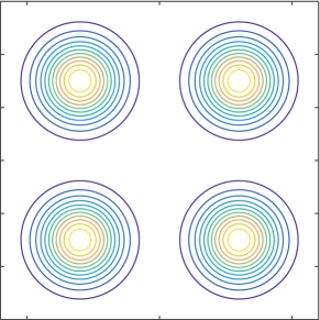
(a) Gaussian mixture

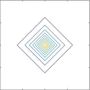
(b) Super-Gaussian

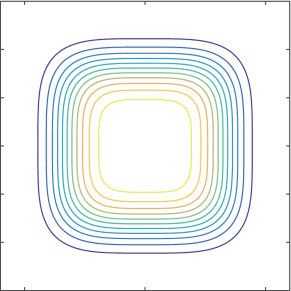
(c) Sub-Gaussian

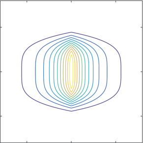
(d) Super- and sub-Gaussian

Figure 2: The two-dimensional distributions of four non-Gaussian densities.

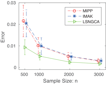
(a) Gaussian mixture

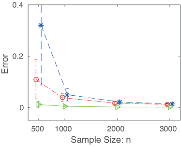
(b) Super-Gaussian

(c) Sub-Gaussian

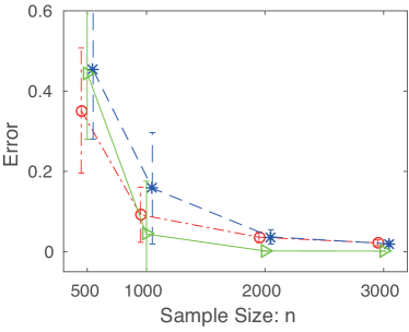
(d) Super- and sub-Gaussian

Figure 3: The average errors over $50$ runs for four kinds of non-Gaussian signal components as the functions of samples size $n$. The error bars denote standard deviations. The horizontal position of the markers for MIPP and IMAK was slightly modified to improve visibility of their error bars.

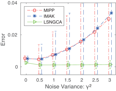
(a) Gaussian mixture

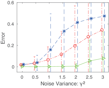
(b) Super-Gaussian

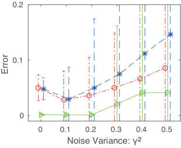
(c) Sub-Gaussian

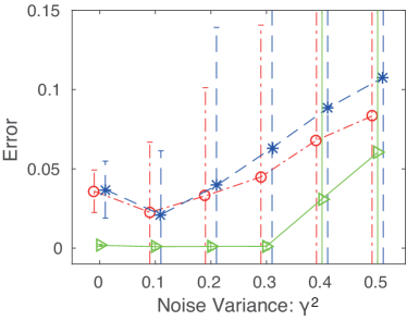
(d) Super- and sub-Gaussian

Figure 4: The average errors over $50$ runs for four kinds of non-Gaussian signal components as the functions of noise variances $\gamma^{2}$ when $n=2,000$. The horizontal position of the markers for MIPP and IMAK was slightly modified to improve visibility of their error bars.

In this section, we experimentally illustrate how LSNGCA works on artificial data, and compare its performance with MIPP and IMAK.

Non-Gaussian signal components $\bm{s}=(s_{1},s_{2})^{\top}$ were sampled from the following distributions:

• Gaussian mixture: $p(s_{1},s_{2})\propto\prod_{i=1}^{2}\exp\{-(s_{i}-3)^{2}/2\}+\exp\{-(s_{i}+3)^{2}/2\}$ (Fig. 2(a)).

• Super-Gaussian: $p(s_{1},s_{2})\propto\prod_{i=1}^{2}\exp\left(-|s_{i}|/\alpha\right)$ where $\alpha$ is determined such that the variances of $s_{1}$ and $s_{2}$ are $3$ (Fig. 2(b)).

• Sub-Gaussian: $p(s_{1},s_{2})\propto\prod_{i=1}^{2}\exp(-s_{i}^{4}/\beta)$ where $\beta$ is determined such that the variances of $s_{1}$ and $s_{2}$ are $3$ (Fig. 2(c)).

• Super- and sub-Gaussian: $p(s_{1},s_{2})=p(s_{1})p(s_{2})$ where $p(s_{1})\propto\exp(-|s_{1}|/\alpha)$ and $p(s_{2})\propto\exp(-s_{2}^{4}/\beta)$. $\alpha$ and $\beta$ is determined such that the variances of $s_{1}$ and $s_{2}$ are $3$ (Fig. 2(d)).

Then, data was generated according to $\bm{x}=(s_{1},s_{2},n_{3},\dots,n_{10})$ where $n_{i}$ for $i=3,\dots,10$ were sampled from the independent standard normal density. The error was measured by

$$\mathcal{E}(\widehat{\mathcal{L}},\mathcal{L})=\frac{1}{d_{\bm{\mathrm{s}}}}\sum_{i=1}^{d_{\bm{\mathrm{s}}}}\|\widehat{\bm{e}}_{i}-\Pi_{\mathcal{L}}\widehat{\bm{e}}_{i}\|^{2},$$

where $\{\widehat{\bm{e}}_{i}\}_{i=1}^{d_{\bm{\mathrm{s}}}}$ is an orthonormal basis of $\widehat{\mathcal{L}}$, and $\Pi_{\mathcal{L}}$ denotes the orthogonal projection on $\mathcal{L}$. For model selection in LSLDG, a five-hold cross-validation was performed with respect to the hold-out error of (10) using the ten candidate values for $\sigma_{j}$ (or $\lambda_{j}$) from $10^{-1}$ (or $10^{-5}$) to $10$ at the regular interval in logarithmic scale .

The results are presented in Fig. 3. For the Gaussian mixture and super-Gaussian cases, LSNGCA always works better than MIPP and IMAK even when the sample size is relatively small (Fig. 3(a) and (b)). On the other hand, when the signal components include sub-Gaussian components and the number of samples is insufficient, the performance of LSNGCA is not good (Fig. 3(c) and (d)). This presumably comes from the fact that estimating the gradients for logarithmic sub-Gaussian densities is more challenging than super-Gaussian densities. However, as long as the number of sample is sufficient, the performance of LSNGCA is comparable to or slightly better than other methods.

Next, we investigate the performance of the three algorithms when the non-Gaussian signal components in data are contaminated by Gaussian noises such that $\bm{x}=(s_{1}+n_{1},s_{2}+n_{2},n_{3},\dots,n_{10})$ where $n_{1}$ and $n_{2}$ are independently sampled from the Gaussian density with the mean $0$ and variance $\gamma^{2}$, while other $n_{i}$ for $i=3,\dots,10$ are sampled as in the last experiment. Fig. 4(a) and (b) show that as $\gamma^{2}$ increases, the estimation errors of LSNGCA for the Gaussian mixture or super-Gaussian distribution more mildly increases than MIPP and IMAK. When the data includes sub-Gaussian components, LSNGCA still works better than MIPP and IMAK for weak noise, but all methods are not robust to stronger noises.

For computational costs, MIPP is the best method, while IMAK consumes much time (Fig.5). MIPP estimates a bunch of $\bm{\beta}_{k}$ by simply computing (4), and FastICA used in MIPP is an iterative method, but its convergence is fast. Therefore, MIPP is a quite efficient method. As reviewed in Section 2.3, because of the alternate and iterative procedure, IMAK is computationally demanding. LSNGCA is less efficient than MIPP, but its computational time is still reasonable.

In short, LSNGCA is advantageous in terms of the sample size and noise tolerance especially when the non-Gaussian signal components follow multi-modal or super-Gaussian distributions. Furthermore, LSNGCA is not the most efficient algorithm, but its computational cost is reasonable.

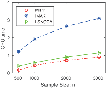
Figure 5: The average CPU time over $50$ runs for the Gaussian mixture as the functions of samples size $n$. The vertical axis is in logarithmic scale.

6 Application to Binary Classification on Benchmark Datasets

In this section, we apply LSNGCA to binary classification on benchmark datasets. For comparison, in addition to MIPP and IMAK, we employed PCA and locality preserving projections (LPP) (He and Niyogi, 2004). For LPP, the nearest-neighbor-based weight matrix were constructed using the heat kernel whose width parameter was fixed to $t_{i}t_{j}$. $t_{i}$ is the Euclidean distance to the $k$-nearest neighbor sample of $\bm{x}_{i}$ and here we set $k=7$ as suggested by Zelnik-Manor and Perona (2005).

We used datasets for binary classification which are available at https://www.csie.ntu.edu.tw/~cjlin/libsvmtools/datasets/. For each dataset, we randomly selected $n$ samples for the training phase. The remaining samples were used for the test phase. For large datasets, we randomly chose $1,000$ samples for the training phase as well as for the test phase. As preprocessing, we separately subtracted the empirical means from the training and test samples. The projection matrix was estimated from the $n$ training samples by each method. Then, the support vector machine (SVM) (Scholkopf and Smola, 2001) was trained using the dimension-reduced training data.

The averages and standard deviations for miss classification rates over $30$ runs are summarized in Table 1. This table shows that LSNGCA overall compares favorably with other algorithms.

Table 1: The averages and standard deviations of misclassification rates for benchmark datasets over $30$ runs. The numbers in the parentheses are standard deviations. The best and comparable methods judged by the unpaired t-test at the significance level $1\%$ are described in boldface. The symbol “-” in the table means that IMAK unexpectedly stopped during the experiments because of a numerical problem.

australian $(d_{\bm{\mathrm{x}}},n)=(14,200)$
	LSNGCA	MIPP	IMAK	PCA	LPP
$d_{\bm{\mathrm{s}}}=2$	20.20(5.09)	21.02(6.66)	33.43(4.99)	17.37(1.30)	17.50(1.08)
$d_{\bm{\mathrm{s}}}=4$	16.23(2.60)	15.90(2.14)	32.53(6.06)	14.92(1.17)	15.07(1.16)
$d_{\bm{\mathrm{s}}}=6$	15.41(2.32)	15.22(2.02)	30.71(5.71)	14.16(1.16)	14.39(1.10)

german.numer $(d_{\bm{\mathrm{x}}},n)=(24,200)$
	LSNGCA	MIPP	IMAK	PCA	LPP
$d_{\bm{\mathrm{s}}}=2$	30.27(0.74)	30.35(0.77)	-	30.63(1.38)	30.82(1.52)
$d_{\bm{\mathrm{s}}}=4$	30.29(0.62)	30.45(0.86)	31.12(1.22)	29.90(1.68)	30.07(1.52)
$d_{\bm{\mathrm{s}}}=6$	30.54(1.01)	30.95(0.90)	31.23(1.12)	29.08(1.43)	29.46(1.09)

liver-disorders $(d_{\bm{\mathrm{x}}},n)=(6,200)$
	LSNGCA	MIPP	IMAK	PCA	LPP
$d_{\bm{\mathrm{s}}}=2$	39.31(3.62)	32.62(3.72)	33.15(5.21)	42.14(2.71)	42.00(2.96)
$d_{\bm{\mathrm{s}}}=4$	32.83(5.15)	32.02(3.67)	35.36(3.32)	42.02(2.64)	42.02(2.71)

SUSY $(d_{\bm{\mathrm{x}}},n)=(18,1000)$
	LSNGCA	MIPP	IMAK	PCA	LPP
$d_{\bm{\mathrm{s}}}=2$	29.58(1.86)	29.42(1.70)	34.37(1.82)	28.71(3.11)	35.26(1.87)
$d_{\bm{\mathrm{s}}}=4$	25.46(2.07)	25.91(1.70)	32.89(2.03)	27.05(1.55)	27.10(2.06)
$d_{\bm{\mathrm{s}}}=6$	23.32(1.73)	24.75(1.61)	31.74(2.16)	25.49(1.50)	25.56(1.56)

shuttle $(d_{\bm{\mathrm{x}}},n)=(9,1000)$
	LSNGCA	MIPP	IMAK	PCA	LPP
$d_{\bm{\mathrm{s}}}=2$	11.29(2.53)	14.39(3.34)	-	16.01(2.20)	11.41(3.53)
$d_{\bm{\mathrm{s}}}=4$	6.04(3.24)	10.45(1.12)	16.84(1.43)	8.18(0.93)	9.36(2.21)
$d_{\bm{\mathrm{s}}}=6$	3.03(1.73)	10.24(1.19)	16.84(1.43)	8.46(1.02)	11.03(2.91)

vehicle $(d_{\bm{\mathrm{x}}},n)=(18,200)$
	LSNGCA	MIPP	IMAK	PCA	LPP
$d_{\bm{\mathrm{s}}}=2$	41.23(4.26)	43.36(3.78)	49.11(2.63)	38.88(2.47)	46.97(2.44)
$d_{\bm{\mathrm{s}}}=4$	35.16(3.76)	34.26(4.13)	50.04(1.42)	38.43(2.16)	45.85(3.11)
$d_{\bm{\mathrm{s}}}=6$	30.72(3.95)	26.60(2.24)	50.33(1.19)	34.30(2.99)	45.47(4.05)

svmguide3 $(d_{\bm{\mathrm{x}}},n)=(21,200)$
	LSNGCA	MIPP	IMAK	PCA	LPP
$d_{\bm{\mathrm{s}}}=2$	22.58(1.55)	23.30(1.38)	-	23.22(1.12)	23.92(0.52)
$d_{\bm{\mathrm{s}}}=4$	22.32(1.59)	21.63(1.28)	23.93(0.52)	21.74(0.92)	23.45(0.75)
$d_{\bm{\mathrm{s}}}=6$	22.20(1.54)	21.29(0.96)	23.92(0.52)	22.06(0.96)	23.53(0.68)

7 Conclusion

In this paper, we proposed a novel algorithm for non-Gaussian component analysis (NGCA) called the least-squares NGCA (LSNGCA). The subspace identification in LSNGCA is performed using the eigenvalue decomposition without any iterative procedures, and thus LSNGCA is computationally reasonable. Through theoretical analysis, we established the optimal convergence rate in a parametric setting for the subspace identification. The experimental results confirmed that LSNGCA performs better than existing algorithms especially for multi-modal or super-Gaussian signal components, and reasonably works on benchmark datasets.

Acknowledgements

Hiroaki Sasaki did most of this work when he was working at the university of Tokyo.

Appendix A Proof of Theorem 1

Our proof can be divided into two parts as mentioned in Section 4.

A.1 Part One: Convergence of LSLDG

A.1.1 Step 1.1

First of all, we establish the growth condition of LSLDG (see Definition 6.1 in Bonnans and Shapiro [1998] for the detailed definition of the growth condition). Denote the expected and empirical objective functions by

$$J_{j}^{*}(\bm{\theta}) =\bm{\theta}^{\top}\mathbf{G}_{j}^{*}\bm{\theta}+2\bm{\theta}^{\top}\bm{h}_{j}^{*}+\lambda_{j}^{*}\bm{\theta}^{\top}\bm{\theta},$$

$$\widehat{J}_{j}(\bm{\theta}) =\bm{\theta}^{\top}\widehat{\mathbf{G}}_{j}\bm{\theta}+2\bm{\theta}^{\top}\widehat{\bm{h}}_{j}+\lambda_{j}\bm{\theta}^{\top}\bm{\theta}.$$

Then $\bm{\theta}_{j}^{*}=\mathop{\rm argmin}\limits\nolimits_{\bm{\theta}}J_{j}^{*}(\bm{\theta})$ and $\widehat{\bm{\theta}}_{j}=\mathop{\rm argmin}\limits\nolimits_{\bm{\theta}}\widehat{J}_{j}(\bm{\theta})$, and we have

Lemma 2.

The following second-order growth condition holds

$$J_{j}^{*}(\bm{\theta})\geq J_{j}^{*}(\bm{\theta}_{j}^{*})+\epsilon_{\lambda}\|\bm{\theta}-\bm{\theta}_{j}^{*}\|_{2}^{2}.$$

Proof.

$J_{j}^{*}(\bm{\theta})$ is strongly convex with parameter at least $2\lambda_{j}^{*}$, since $\mathbf{G}_{j}^{*}$ is symmetric and positive-definite. Hence,

$$J_{j}^{*}(\bm{\theta}) \geq J_{j}^{*}(\bm{\theta}_{j}^{*})+(\nabla J_{j}^{*}(\bm{\theta}_{j}^{*}))^{\top}(\bm{\theta}-\bm{\theta}_{j}^{*})+\lambda_{j}^{*}\|\bm{\theta}-\bm{\theta}_{j}^{*}\|_{2}^{2}$$

$$\geq J_{j}^{*}(\bm{\theta}_{j}^{*})+\epsilon_{\lambda}\|\bm{\theta}-\bm{\theta}_{j}^{*}\|_{2}^{2},$$

where we used the optimality condition $\nabla J_{j}^{*}(\bm{\theta}_{j}^{*})=\bm{0}$ and the first condition $\lambda_{j}^{*}\geq\epsilon_{\lambda}$ of the theorem. ∎

A.1.2 Step 1.2

Second, we study the stability (with respect to perturbation) of $J_{j}^{*}(\bm{\theta})$ at $\bm{\theta}_{j}^{*}$. Let

$$\bm{u}=\{\bm{u}_{G}\in\mathcal{S}_{+}^{b},\bm{u}_{h}\in\mathbb{R}^{b},u_{\lambda}\in\mathbb{R}\}$$

be a set of perturbation parameters, where $b$ is the number of centers in $\psi_{ij}(\bm{x})$ and $\mathcal{S}_{+}^{b}\subset\mathbb{R}^{b\times b}$ is the cone of $b$-by-$b$ symmetric positive semi-definite matrices. Define our perturbed objective function by

$$J_{j}(\bm{\theta},\bm{u})=\bm{\theta}^{\top}(\mathbf{G}_{j}^{*}+\bm{u}_{G})\bm{\theta}+2\bm{\theta}^{\top}(\bm{h}_{j}^{*}+\bm{u}_{h})+(\lambda_{j}^{*}+u_{\lambda})\bm{\theta}^{\top}\bm{\theta}.$$

It is clear that $J_{j}^{*}(\bm{\theta})=J_{j}(\bm{\theta},\bm{0})$, and then the stability of $J_{j}^{*}(\bm{\theta})$ at $\bm{\theta}_{j}^{*}$ can be characterized as follows.

Lemma 3.

The difference function $J_{j}(\cdot,\bm{u})-J_{j}^{*}(\cdot)$ is Lipschitz continuous modulus

$$\omega(\bm{u})=\mathcal{O}(\|\bm{u}_{G}\|_{\mathrm{Fro}}+\|\bm{u}_{h}\|_{2}+|u_{\lambda}|)$$

on a sufficiently small neighborhood of $\bm{\theta}_{j}^{*}$.

Proof.

The difference function is

$$J_{j}(\bm{\theta},\bm{u})-J_{j}^{*}(\bm{\theta})=\bm{\theta}^{\top}\bm{u}_{G}\bm{\theta}+2\bm{\theta}^{\top}\bm{u}_{h}+u_{\lambda}\bm{\theta}^{\top}\bm{\theta},$$

with a partial gradient

$$\frac{\partial}{\partial\bm{\theta}}(J_{j}(\bm{\theta},\bm{u})-J_{j}^{*}(\bm{\theta}))=2\bm{u}_{G}\bm{\theta}+2\bm{u}_{h}+2u_{\lambda}\bm{\theta}.$$

Notice that due to the $\ell_{2}$-regularization in $J_{j}^{*}(\bm{\theta})$, $\exists M>0$ such that $\|\bm{\theta}_{j}^{*}\|_{2}\leq M$. Now given a $\delta$-ball of $\bm{\theta}_{j}^{*}$, i.e., $B_{\delta}(\bm{\theta}_{j}^{*})=\{\bm{\theta}\mid\|\bm{\theta}-\bm{\theta}_{j}^{*}\|_{2}\leq\delta\}$, it is easy to see that $\forall\bm{\theta}\in B_{\delta}(\bm{\theta}_{j}^{*})$,

$$\|\bm{\theta}\|_{2}\leq\|\bm{\theta}-\bm{\theta}_{j}^{*}\|_{2}+\|\bm{\theta}_{j}^{*}\|_{2}\leq\delta+M,$$

and consequently

$$\left\|\frac{\partial}{\partial\bm{\theta}}(J_{j}(\bm{\theta},\bm{u})-J_{j}^{*}(\bm{\theta}))\right\|_{2}\leq 2(\delta+M)(\|\bm{u}_{G}\|_{\mathrm{Fro}}+|u_{\lambda}|)+2\|\bm{u}_{h}\|_{2}.$$

This says that the gradient $\frac{\partial}{\partial\bm{\theta}}(J_{j}(\bm{\theta},\bm{u})-J_{j}^{*}(\bm{\theta}))$ has a bounded norm of order $\mathcal{O}(\|\bm{u}_{G}\|_{\mathrm{Fro}}+\|\bm{u}_{h}\|_{2}+|u_{\lambda}|)$, and proves that the difference function $J_{j}(\bm{\theta},\bm{u})-J_{j}^{*}(\bm{\theta})$ is Lipschitz continuous on the ball $B_{\delta}(\bm{\theta}_{j}^{*})$, with a Lipschitz constant of the same order. ∎

A.1.3 Step 1.3

Intuitively, Lemma 2 guarantees that the unperturbed objective function $J_{j}^{*}(\bm{\theta})$ grows quickly when $\bm{\theta}$ leaves $\bm{\theta}_{j}^{*}$. Lemma 3 guarantees that the perturbed objective function $J_{j}(\bm{\theta},\bm{u})$ changes slowly for $\bm{\theta}$ around $\bm{\theta}_{j}^{*}$, where the slowness is with respect to the perturbation $\bm{u}$ it suffers. Based on Lemma 2, Lemma 3, and Proposition 6.1 in Bonnans and Shapiro [1998],

$$\|\widehat{\bm{\theta}}_{j}-\bm{\theta}_{j}^{*}\|_{2}\leq\frac{\omega(\bm{u})}{\epsilon_{\lambda}}=\mathcal{O}(\|\bm{u}_{G}\|_{\mathrm{Fro}}+\|\bm{u}_{h}\|_{2}+|u_{\lambda}|),$$

since $\widehat{\bm{\theta}}_{j}$ is the exact solution to $\widehat{J}_{j}(\bm{\theta})=J_{j}(\bm{\theta},\bm{u})$ given $\bm{u}_{G}=\widehat{\mathbf{G}}_{j}-\mathbf{G}_{j}^{*}$, $\bm{u}_{h}=\widehat{\mathbf{h}}_{j}-\mathbf{h}_{j}^{*}$, and $u_{\lambda}=\lambda_{j}-\lambda_{j}^{*}$.

According to the central limit theorem (CLT), $\|\bm{u}_{G}\|_{\mathrm{Fro}}=\mathcal{O}_{p}(n^{-1/2})$ and $\|\bm{u}_{h}\|_{2}=\mathcal{O}_{p}(n^{-1/2})$. Furthermore, we have already assumed that $|u_{\lambda}|=\mathcal{O}(n^{-1/2})$ in the first condition of the theorem. Hence, as $n\to\infty$,

$$\|\widehat{\bm{\theta}}_{j}-\bm{\theta}_{j}^{*}\|_{2}=\mathcal{O}_{p}\left(n^{-1/2}\right).$$ (11)

A.1.4 Step 1.4

Considering the empirical estimate of the log-density gradient $\widehat{g}^{(j)}(\bm{x})$ and the optimal estimate of the log-density gradient $g^{*(j)}(\bm{x})$, their gap in terms of the infinity norm is bounded below:

$$\|\widehat{g}^{(j)}-g^{*(j)}\|_{\infty} =\sup\nolimits_{\bm{x}}|\widehat{g}^{(j)}(\bm{x})-g^{*(j)}(\bm{x})|$$

$$=\sup\nolimits_{\bm{x}}|(\widehat{\bm{\theta}}_{j}-\bm{\theta}_{j}^{*})^{\top}\bm{\psi}_{j}(\bm{x})|$$

$$\leq\|\widehat{\bm{\theta}}_{j}-\bm{\theta}_{j}^{*}\|_{2}\cdot\sup\nolimits_{\bm{x}}\|\bm{\psi}_{j}(\bm{x})\|_{2},$$

where the Cauchy-Schwarz inequality is used. Recall that $\bm{c}_{1},\ldots,\bm{c}_{b}$ are the centers, and for any $i$,

$$|\psi_{ij}(\bm{x})|=\frac{|[\bm{c}_{i}-\bm{x}]^{(j)}|}{\sigma_{j}^{2}}\exp\left(-\frac{\|\bm{x}-\bm{c}_{i}\|_{2}^{2}}{2\sigma_{j}^{2}}\right)\leq\frac{|[\bm{c}_{i}-\bm{x}]^{(j)}|}{\sigma_{j}^{2}}\left(-\frac{([\bm{x}-\bm{c}_{i}]^{(j)})^{2}}{2\sigma_{j}^{2}}\right).$$

It is obvious that $|\psi_{ij}(\bm{x})|$ is bounded, since $\exp(-z^{2})$ converges to zero much faster than $|z|$ diverges to infinity. Therefore, $\sup_{\bm{x}}\|\bm{\psi}_{j}(\bm{x})\|_{2}$ is a finite number, and we could know from Eq. (11) that

$$\|\widehat{g}^{(j)}-g^{*(j)}\|_{\infty}\leq\mathcal{O}(\|\widehat{\bm{\theta}}_{j}-\bm{\theta}_{j}^{*}\|_{2})=\mathcal{O}_{p}\left(n^{-1/2}\right).$$ (12)

A.2 Part Two: Convergence of LSNGCA

A.2.1 Step 2.1

To begin with, we focus on the convergence of $\widehat{\mathbf{\Gamma}}$. Given any $\bm{y}$, let $\widehat{\bm{z}}=\widehat{\bm{g}}(\bm{y})$ and $\bm{z}^{*}=\bm{g}^{*}(\bm{y})$, then

$$(\widehat{\bm{z}}+\bm{y})(\widehat{\bm{z}}+\bm{y})^{\top}-(\bm{z}^{*}+\bm{y})(\bm{z}^{*}+\bm{y})^{\top} =\widehat{\bm{z}}\widehat{\bm{z}}^{\top}-\bm{z}^{*}\bm{z}^{*\top}+(\widehat{\bm{z}}-\bm{z}^{*})\bm{y}^{\top}+\bm{y}(\widehat{\bm{z}}-\bm{z}^{*})^{\top}$$

$$=(\widehat{\bm{z}}-\bm{z}^{*})\widehat{\bm{z}}^{\top}+\bm{z}^{*}(\widehat{\bm{z}}-\bm{z}^{*})^{\top}+(\widehat{\bm{z}}-\bm{z}^{*})\bm{y}^{\top}+\bm{y}(\widehat{\bm{z}}-\bm{z}^{*})^{\top}.$$

As a result, based on Eq. (12),

$$\|(\widehat{\bm{z}}+\bm{y})(\widehat{\bm{z}}+\bm{y})^{\top}-(\bm{z}^{*}+\bm{y})(\bm{z}^{*}+\bm{y})^{\top}\|_{\mathrm{Fro}} \leq\|(\widehat{\bm{z}}-\bm{z}^{*})\widehat{\bm{z}}^{\top}\|_{\mathrm{Fro}}+\|\bm{z}^{*}(\widehat{\bm{z}}-\bm{z}^{*})^{\top}\|_{\mathrm{Fro}}$$

$$\quad+\|(\widehat{\bm{z}}-\bm{z}^{*})\bm{y}^{\top}\|_{\mathrm{Fro}}+\|\bm{y}(\widehat{\bm{z}}-\bm{z}^{*})^{\top}\|_{\mathrm{Fro}}$$

$$\leq(\|\widehat{\bm{z}}\|_{2}+\|\bm{z}^{*}\|_{2}+2\|\bm{y}\|)\cdot\|\widehat{\bm{z}}-\bm{z}^{*}\|_{2}$$

$$=\mathcal{O}(\|\widehat{\bm{z}}-\bm{z}^{*}\|_{2})$$

$$=\mathcal{O}_{p}\left(n^{-1/2}\right).$$

This has proved the point-wise convergence from $(\widehat{\bm{g}}(\bm{y})+\bm{y})(\widehat{\bm{g}}(\bm{y})+\bm{y})^{\top}$ to $(\bm{g}^{*}(\bm{y})+\bm{y})(\bm{g}^{*}(\bm{y})+\bm{y})^{\top}$.

Define an intermediate matrix based on $\bm{y}_{1},\ldots,\bm{y}_{n}$ as

$$\widetilde{\mathbf{\Gamma}}=\frac{1}{n}\sum_{i=1}^{n}(\bm{g}^{*}(\bm{y}_{i})+\bm{y}_{i})(\bm{g}^{*}(\bm{y}_{i})+\bm{y}_{i})^{\top}.$$

Subsequently, $\widehat{\mathbf{\Gamma}}$ converges to $\widetilde{\mathbf{\Gamma}}$ in $\mathcal{O}_{p}(n^{-1/2})$ due to the point-wise convergence from $(\widehat{\bm{g}}(\bm{y})+\bm{y})(\widehat{\bm{g}}(\bm{y})+\bm{y})^{\top}$ to $(\bm{g}^{*}(\bm{y})+\bm{y})(\bm{g}^{*}(\bm{y})+\bm{y})^{\top}$ that was just proved, and $\widetilde{\mathbf{\Gamma}}$ converges to $\mathbf{\Gamma}^{*}$ in $\mathcal{O}_{p}(n^{-1/2})$ due to CLT. A combination of these two results gives us

$$\|\widehat{\mathbf{\Gamma}}-\mathbf{\Gamma}^{*}\|_{\mathrm{Fro}}\leq\|\widehat{\mathbf{\Gamma}}-\widetilde{\mathbf{\Gamma}}\|_{\mathrm{Fro}}+\|\widetilde{\mathbf{\Gamma}}-\mathbf{\Gamma}^{*}\|_{\mathrm{Fro}}=\mathcal{O}_{p}\left(n^{-1/2}\right).$$ (13)

A.2.2 Step 2.2

Now let us consider the eigenvalues of $\mathbf{\Gamma}^{*}$. Let $\mu_{1}>\cdots>\mu_{r}>\mu_{r+1}$ be the first $r+1$ eigenvalues of $\mathbf{\Gamma}^{*}$ counted without multiplicity, such that $\mu_{r}$ is the $d_{\bm{\mathrm{s}}}$-th largest eigenvalue of $\mathbf{\Gamma}^{*}$ if counted with multiplicity. Define the eigen-gap by

$$\epsilon_{\mu}=\min_{i=1,\ldots,r}\{\mu_{i}-\mu_{i+1}\}.$$

We have assumed that $\mu_{1}<+\infty$ and $\mu_{r}>0$ in the second condition of the theorem, and thus it must hold that $0<\epsilon_{\mu}<+\infty$. In the case that $\mathbf{\Gamma}^{*}$ has only one eigenvalue, we can simply assign $\epsilon_{\mu}=1$.

According to Lemma 5.2 of Koltchinskii and Giné [2000] as well as the appendix of Koltchinskii [1998], we can derive the stability of the eigen-decomposition of $\mathbf{\Gamma}^{*}$ with respect to some perturbation $\bm{u}_{\Sigma}=\widehat{\mathbf{\Gamma}}-\mathbf{\Gamma}^{*}$. Whenever $\|\bm{u}_{\Sigma}\|_{\mathrm{Fro}}<\epsilon_{\mu}/4$:

• The first $r+1$ eigenvalues $\mu_{1}^{\prime}>\cdots>\mu_{r}^{\prime}>\mu_{r+1}^{\prime}$ of $\widehat{\mathbf{\Gamma}}=\mathbf{\Gamma}^{*}+\bm{u}_{\Sigma}$, counted without multiplicity, satisfy that $|\mu_{i}^{\prime}-\mu_{i}|\leq\|\bm{u}_{\Sigma}\|_{\mathrm{Fro}}$ for $1\leq i\leq r$, and $\mu_{r}-\mu_{r+1}^{\prime}\geq\epsilon_{\mu}-\|\bm{u}_{\Sigma}\|_{\mathrm{Fro}}$;

• Denote by $\Pi_{i}(\mathbf{\Gamma}^{*})$ the orthogonal projection onto the eigen-spaces of $\mathbf{\Gamma}^{*}$ associated with $\mu_{i}$, and by $\Pi_{i}(\widehat{\mathbf{\Gamma}})$ that of $\widehat{\mathbf{\Gamma}}=\mathbf{\Gamma}^{*}+\bm{u}_{\Sigma}$ associated with $\mu_{i}^{\prime}$, then for $1\leq i\leq r$,

  $$\|\Pi_{i}(\widehat{\mathbf{\Gamma}})-\Pi_{i}(\mathbf{\Gamma}^{*})\|_{\mathrm{Fro}}\leq\frac{4}{\epsilon_{\mu}}\|\bm{u}_{\Sigma}\|_{\mathrm{Fro}}.\vspace{-1ex}$$

We have employed simplified notations above to avoid sophisticated names in operator theory. Intuitively, the first item guarantees that the eigenvalues of the perturbed matrix $\widehat{\mathbf{\Gamma}}$ are close to that of $\mathbf{\Gamma}^{*}$, and the second item guarantees that the eigen-spaces of $\widehat{\mathbf{\Gamma}}$ are also close to that of $\mathbf{\Gamma}^{*}$.

By noting that $\|\widehat{\mathbf{\Gamma}}-\mathbf{\Gamma}^{*}\|_{\mathrm{Fro}}$ was shown to have an order of $\mathcal{O}_{p}(n^{-1/2})$ in (13), whereas the eigen-gap $\epsilon_{\mu}$ for fixed $\mathbf{\Gamma}^{*}$ is a constant value, we could obtain that as $n\to\infty$ for all $i$,

$$\|\Pi_{i}(\widehat{\mathbf{\Gamma}})-\Pi_{i}(\mathbf{\Gamma}^{*})\|_{\mathrm{Fro}}=\mathcal{O}_{p}\left(n^{-1/2}\right).$$ (14)

A.2.3 Step 2.3

Finally, we can bound $\mathcal{D}(\widehat{\mathcal{L}},\mathcal{L}^{*})$. The eigenvalues of $\mathbf{\Gamma}^{*}$ and $\widehat{\mathbf{\Gamma}}$ were counted without multiplicity, and hence the bases of $\Pi_{i}(\widehat{\mathbf{\Gamma}})$ and $\Pi_{i}(\mathbf{\Gamma}^{*})$ may not be unique. Nevertheless, let $\mathbf{E}_{\mathcal{I}^{*}}$ be the matrix form of a fixed orthonormal basis of $\mathcal{I}^{*}$, then there exists a sequence of matrices $\{\mathbf{E}_{\widehat{\mathcal{I}},1},\ldots,\mathbf{E}_{\widehat{\mathcal{I}},n},\ldots\}$ such that

• $\mathbf{E}_{\widehat{\mathcal{I}},n}$ is the matrix form of a certain orthonormal basis of $\widehat{\mathcal{I}}$ based on a set of data samples of size $n$;

• The sequence converges to $\mathbf{E}_{\mathcal{I}^{*}}$ in $\mathcal{O}_{p}(n^{-1/2})$, i.e.,

  $$\|\mathbf{E}_{\widehat{\mathcal{I}},n}-\mathbf{E}_{\mathcal{I}^{*}}\|_{\mathrm{Fro}}=\mathcal{O}_{p}\left(n^{-1/2}\right),\vspace{-1ex}$$ (15)

based on Eq. (14). Denote by $\mathbf{E}_{\mathcal{L}^{*}}=\bm{\Sigma}^{-1/2}\mathbf{E}_{\mathcal{I}^{*}}$ and $\mathbf{E}_{\widehat{\mathcal{L}},n}=\widehat{\bm{\Sigma}}^{-1/2}\mathbf{E}_{\widehat{\mathcal{I}},n}$, and then

$$\mathbf{E}_{\widehat{\mathcal{L}},n}-\mathbf{E}_{\mathcal{L}^{*}}=\widehat{\bm{\Sigma}}^{-1/2}\mathbf{E}_{\widehat{\mathcal{I}},n}-\bm{\Sigma}^{-1/2}\mathbf{E}_{\mathcal{I}^{*}}=(\widehat{\bm{\Sigma}}^{-1/2}-\bm{\Sigma}^{-1/2})\mathbf{E}_{\widehat{\mathcal{I}},n}+\bm{\Sigma}^{-1/2}(\mathbf{E}_{\widehat{\mathcal{I}},n}-\mathbf{E}_{\mathcal{I}^{*}}).$$

Therefore, we can prove that

$$\mathcal{D}(\widehat{\mathcal{L}},\mathcal{L}^{*}) =\inf\nolimits_{\widehat{\mathbf{E}},\mathbf{E}^{*}}\|\widehat{\mathbf{E}}-\mathbf{E}^{*}\|_{\mathrm{Fro}}$$

$$\leq\|\mathbf{E}_{\widehat{\mathcal{L}},n}-\mathbf{E}_{\mathcal{L}^{*}}\|_{\mathrm{Fro}}$$

$$\leq\|\mathbf{E}_{\widehat{\mathcal{I}},n}\|_{\mathrm{Fro}}\cdot\|\widehat{\bm{\Sigma}}^{-1/2}-\bm{\Sigma}^{-1/2}\|_{\mathrm{Fro}}+\|\bm{\Sigma}^{-1/2}\|_{\mathrm{Fro}}\cdot\|\mathbf{E}_{\widehat{\mathcal{I}},n}-\mathbf{E}_{\mathcal{I}^{*}}\|_{\mathrm{Fro}}$$

$$=\mathcal{O}(\|\widehat{\bm{\Sigma}}^{-1/2}-\bm{\Sigma}^{-1/2}\|_{\mathrm{Fro}})+\mathcal{O}(\|\mathbf{E}_{\widehat{\mathcal{I}},n}-\mathbf{E}_{\mathcal{I}^{*}}\|_{\mathrm{Fro}})$$

$$=\mathcal{O}_{p}\left(n^{-1/2}\right),$$

according to CLT and Eq. (15). ∎

References

- Blanchard et al. (2006) G. Blanchard, M. Kawanabe, M. Sugiyama, V. Spokoiny, and K. Müller. In search of non-Gaussian components of a high-dimensional distribution. Journal of Machine Learning Research, 7:247–282, 2006.
- Bonnans and Cominetti (1996) F. Bonnans and R. Cominetti. Perturbed optimization in Banach spaces I: A general theory based on a weak directional constraint qualification; II: A theory based on a strong directional qualification condition; III: Semiinfinite optimization. SIAM Journal on Control and Optimization, 34:1151–1171, 1172–1189, and 1555–1567, 1996.
- Bonnans and Shapiro (1998) F. Bonnans and A. Shapiro. Optimization problems with perturbations, a guided tour. SIAM Review, 40(2):228–264, 1998.
- Chang and Lin (2011) C. Chang and C. Lin. LIBSVM: A library for support vector machines. ACM Transactions on Intelligent Systems and Technology, 2:27:1–27:27, 2011. Software available at http://www.csie.ntu.edu.tw/~cjlin/libsvm.
- Comon (1994) P. Comon. Independent component analysis, a new concept? Signal Processing, 36(3):287–314, 1994.
- Cox (1985) D. D. Cox. A penalty method for nonparametric estimation of the logarithmic derivative of a density function. Annals of the Institute of Statistical Mathematics, 37(1):271–288, 1985.
- Friedman and Tukey (1974) J. Friedman and J. Tukey. A projection pursuit algorithm for exploratory data analysis. IEEE Transactions on Computers, 23(9):881–890, 1974.
- He and Niyogi (2004) X. He and P. Niyogi. Locality preserving projections. In Advances in Neural Information Processing Systems, pages 153–160, 2004.
- Huber (1985) P. Huber. Projection pursuit. The Annals of Statistics, 13(2):435–475, 1985.
- Hyvärinen (1999) A. Hyvärinen. Fast and robust fixed-point algorithms for independent component analysis. IEEE Transactions on Neural Networks, 10(3):626–634, 1999.
- Hyvärinen et al. (2001) A. Hyvärinen, J. Karhunen, and E. Oja. Independent component analysis. John Wiley & Sons, 2001.
- Kawanabe et al. (2007) M. Kawanabe, M. Sugiyama, G. Blanchard, and K. Müller. A new algorithm of non-Gaussian component analysis with radial kernel functions. Annals of the Institute of Statistical Mathematics, 59(1):57–75, 2007.
- Koltchinskii (1998) V. Koltchinskii. Asymptotics of spectral projections of some random matrices approximating integral operators. Progress in Probabilty, 43:191–227, 1998.
- Koltchinskii and Giné (2000) V. Koltchinskii and E. Giné. Random matrix approximation of spectra of integral operators. Bernoulli, 6:113–167, 2000.
- Sasaki et al. (2014) H. Sasaki, A. Hyvärinen, and M. Sugiyama. Clustering via mode seeking by direct estimation of the gradient of a log-density. In Machine Learning and Knowledge Discovery in Databases Part III- European Conference, ECML/PKDD 2014, volume 8726, pages 19–34, 2014.
- Scholkopf and Smola (2001) B. Scholkopf and A. Smola. Learning with kernels: support vector machines, regularization, optimization, and beyond. The MIT press, 2001.
- Sugiyama et al. (2008) M. Sugiyama, M. Kawanabe, G. Blanchard, and K. Müller. Approximating the best linear unbiased estimator of non-Gaussian signals with Gaussian noise. IEICE transactions on information and systems, 91(5):1577–1580, 2008.
- Theis and Kawanabe (2006) F. Theis and M. Kawanabe. Uniqueness of non-Gaussian subspace analysis. In Lecture Notes in Computer Science, volume 3889, pages 917–925. Springer-Verlag, 2006.
- Zelnik-Manor and Perona (2005) L. Zelnik-Manor and P. Perona. Self-tuning spectral clustering. In Advances in Neural Information Processing Systems, pages 1601–1608, 2005.