A Grassmannian Graph Approach to Affine Invariant Feature Matching

Abstract

In this work, we present a novel and practical approach to address one of the longstanding problems in computer vision: 2D and 3D affine invariant feature matching. Our Grassmannian Graph (GrassGraph) framework employs a two stage procedure that is capable of robustly recovering correspondences between two unorganized, affinely related feature (point) sets. The first stage maps the feature sets to an affine invariant Grassmannian representation, where the features are mapped into the same subspace. It turns out that coordinate representations extracted from the Grassmannian differ by an arbitrary orthonormal matrix. In the second stage, by approximating the Laplace-Beltrami operator (LBO) on these coordinates, this extra orthonormal factor is nullified, providing true affine-invariant coordinates which we then utilize to recover correspondences via simple nearest neighbor relations. The resulting GrassGraph algorithm is empirically shown to work well in non-ideal scenarios with noise, outliers, and occlusions. Our validation benchmarks use an unprecedented 440,000+ experimental trials performed on 2D and 3D datasets, with a variety of parameter settings and competing methods. State-of-the-art performance in the majority of these extensive evaluations confirm the utility of our method.

1 Introduction

Feature matching has been a vital component of computer vision since Fischler and Elschlager’s seminal work in 1973 [10]. Since that beginning, there have been torrents of work in this area making it almost impossible to characterize or synthesize. Given this voluminous previous work, it’s understandable if one adopts a perspective that the bar is too high for new ideas. Our goal in the present work is to belie that opinion, clearly demonstrating a novel approach which is simultaneously new (to the best of our knowledge) and easy to implement. Graph representations abound in computer vision. The very first matching work featured a relational graph representation [10], invariant under rigid shape transformations. Within this subfield, there again exist innumerable works with extensions, new formulations, algorithms and the like. Graph representations lead to graph matching—which despite being NP-hard [37]—has attracted a huge amount of attention over the decades.

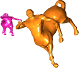
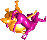
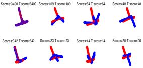
Original Affine Shapes	Grassmannian Representation	LBO Eigenvector Representation with Sign-flips

Figure 1: Visual overview of the GrassGraph algorithm. On the far left, we begin with the original shapes which differ by an affine transform. Moving to the right, the Grassmannian representation stage—constructed via a SVD on the coordinates—removes the affine transformation, leaving only a rotation between the shapes. Next, in our second stage, we approximate the Laplace-Beltrami operator (LBO) on these invariant coordinates and compute its eigenvectors to obtain a set of coordinates that are invariant to isometries (which includes rotations). Finally, we correct for the sign ambiguties that arise from the eigenvector computations. To choose the correct sign flips, a number of mutual nearest neighbor correspondences are computed and the flip combination with the highest score is chosen. The proposed GrassGraph approach is able to recover dense correspondences with the same identical steps applicable to either 2D or 3D data.

Graph representations have also been extended to include invariances under similarity transformations [31] and lately have surfaced in non-rigid matching situations as well [38]. However, in the present work, our focus is on affine invariance. In particular, we introduce both a new Grassmannian Graph representation and an attendant set of affine invariant feature coordinates. We believe this combination to be both novel and useful in feature matching and indexing applications.

Invariants in computer vision have seen better days. While they were the flavor du jour in the early ’90s, with work ranging from geometric hashing [17] to generalized Hough transforms [1], recently this work has not seen much development. Invariants were not robust to missing features and they could not easily be extended to non-rigid matching situations. We speculate, however, that an important additional reason why invariants did not see wide adoption was due to the absence of invariant feature coordinate systems. For example, there were relatively few attempts at creating similarity transformation invariant coordinates from a set of features leading to simpler correspondence finding algorithms (such as nearest neighbor). It is not surprising that it is exactly this aspect of invariance which has seen a resurgence in the past few years [27].

While the idea of constructing new similarity transformation-invariant coordinates dates back earlier, it is only in recent years that it has become commonplace to see new coordinates built out of discrete Laplace-Beltrami Operator (LBO) eigenvectors [16, 28]. The basic idea is extremely straightforward: construct a weighted graph representation from a set of features and then use the principal component eigenvectors of the graph (interpreted as a linear operator) to complete the construction. These new coordinates can then be pressed into service in matching and indexing applications. However, note the fundamental limitation to similarity transformations: can this approach be extended to affine invariance while remaining somewhat robust in the face of noise and outliers?

We answer in the affirmative. In this work, we begin with the original feature set and first construct the Grassmannian. The Grassmannian [3] is a geometric object with the property that all linear combinations of the feature coordinates remain in the same Grassmannian subspace. Therefore a single element of the Grassmannian can be considered to be an affine invariant equivalence class of feature sets. Further, Grassmannians are homeomorphic to orthogonal projection matrices with the latter available for the construction of new affine invariant coordinates. Consequently, the first stage in our construction of affine invariant coordinates is the Grassmannian representation (GR) utilizing orthogonal projection matrices computed from each feature set. Unfortunately, it turns out that two factorizations of projection matrices can differ by an unknown orthonormal matrix. To circumvent this problem, in a second stage, we construct a weighted graph which is invariant to this additional orthonormal factor and then use LBO principal components (as outlined above) to obtain new affine invariant coordinates. Given two sets of features, finding good correspondences is considerably easier in this representation since the affine invariant coordinates lead to efficient nearest neighbor correspondences. The twin strands of research married in our approach are therefore (i) affine invariant Grassmannian representations and (ii) LBO-based weighted graphs resulting in the GrassGraph algorithm for affine invariant feature matching. We believe this combination to be novel and useful and a visual representation of the algorithm is shown in Figure 1.

More than 440,000 experiments conducted in the present work buttress our claims. We take the outlier problems faced by invariant representations very seriously since they derailed previous work (from the early ’90s). We also conduct realistic experiments in the presence of noise, missing points and outliers—on a greater scale than we have seen in comparable related work. Comparisons are conducted against state-of-the-art feature matching algorithms. In this way, we hope to have made the case for the affine invariant representation and new shape coordinates. The ease of implementation and use should pave the way for the Grassmannian Graph representation to be widely used in feature matching and indexing applications.

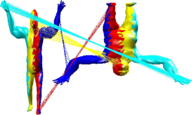
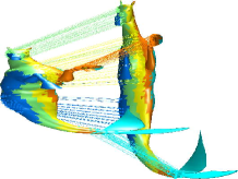
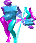
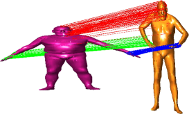
Figure 2: Correspondence recovery on 3D affine shapes and one articulated trial using the proposed GrassGraph algorithm. Note, that we recover dense correspondences but only a subset of the matching points are shown for visualization purposes.

2 Related Work

As mentioned previously the corpus related to affine invariance and graph matching is quite vast, here we highlight the most relevant and early pioneering works that have paved the way for the current method. Umeyama [33] pioneered spectral approaches for the weighted graph matching problem, with several other spectral methods proposed in [4, 6, 20, 22, 30]. After Umeyama, Scott and Longuet-Higgins [29] designed an inter-image proximity matrix between landmarks using Gaussian functions, then solve for correspondences via the singular value decomposition (SVD) to match sets of rigid points. This work was extended by Shapiro [30] to find correspondences on the eigenvectors themselves and overcome the invariance to rotation limitation of the work in [29]. Carcassoni [5, 6] extended the Gaussian kernel to other robust weighting functions and proposed a probabilistic framework for point-to-point matching. In [14], the Laplacian embedding is used to embed 3-D meshes using a global geodesic distance where these embeddings are matched using the ICP algorithm [36]. Mateus [21] used a subset of Laplacian eigenfunctions to perform dense registration between articulated point sets. Once in the eigenspace, the registration was solved using unsupervised clustering and the EM algorithm. All of these previous methods used an eigenvector decomposition to solve the point matching problem under different transformations: translation, rotation, scale and shear, but none are truly affine invariant nor do they produce affine invariant coordinates. In addition, establishing correspondence in the related feature spaces require more complicated methods versus our simple nearest neighbor matching to recover correspondences (even in the presence of noise and outliers).

Another way to address the affine invariance problem is through multi-step approaches which provide invariance to particular transformations at each step. Ha and Moura [11] recovered an intrinsic shape which is invariant to affine-permutation distortions, and use the steps of centering, reshaping, reorientation and sorting. Dalal et al. [8] constructed a rough initial correspondence between two 3D shape surfaces by removing translation, scale, and rotation. They then used a landmark-sliding algorithm based on 3D thin-plate splines (TPS) to model the shape correspondence errors and achieve affine invariance. The methods [8, 11] stepwise construct their affine invariance by targeting individual transformations whereas our subspace method is a true invariant to the entire class of affine transformations. Ho et al. [12] proposed an elegant noniterative algorithm for 2D affine registration by searching for the roots of the associated polynomials. Unfortunately, this method does not generalize to higher dimensions.

Begelfor and Werman [2] popularized the use of Grassmannian subspaces as an affine invariant. Their work focused on developing clustering algorithms on the Grassmann manifold, but they did not utilize this invariance to solve the correspondence problem. A method that did try to address this correspondence problem through subspace invariance was [34]. The robustness of their method was never evaluated, and, moreover, their approach of using QR factorizations of rank-deficient orthogonal projection matrices is quite different from our proposed two-stage approach. Finally, Chellappa et al. have shown the effectiveness of Grassmannian representations for object recognition [32] and their use has expanded to other vision domains [19].

Algorithms that address non-rigid transformations inherently have an advantage over strictly affine methods, here we highlight some notable non-rigid methods that can be used to address the affine correspondence problem. Raviv et al. [26] form an equi-affine (volume preserving) invariant Laplacian for surfaces, with applications in shape matching. Their method, however, requires explicit metric tensor calculations on mesh surfaces which can lead to further complications of singular points on the surfaces. We avoid surfaces parameterization issues, offering an approach that works directly on point sets. Popular non-rigid matching algorithms include CPD [24], gmmreg [15] and TPS-RPM [7]. Graph matching methods have also been quite popular recently. Zhou and de la Torre [37, 38] presented the factorized graph matching (FGM) algorithm in which the affinity matrix is factorized as a Kronecker product of smaller matrices. Although the factorization of affinity matrices makes large graph matching problems more tractable, the method is still computationally expensive.

3 Grassmannians and Affine Invariance

The principal contributions of this work are (i) a Grassmannian representation (GR) of feature vectors and (ii) new affine invariant coordinates in which feature correspondences can be sought. Below, we describe both the intuitive and formal aspects of the new representation.

3.1 Formulation

Let $X\in\mathbb{R}^{N\times D}$ denote a set of $N$ features living in a $D$ dimensional space (with $D=2$ or 3). The application of an affine transformation on the feature set $X$ can be written as

$$\tilde{X}=XA+\mathbf{1}T$$ (1)

where $A\in\mathbb{R}^{D\times D}$ and $T\in\mathbb{R}^{D}$ are the multiplicative and additive aspects of the affine transformation. The matrix $A$ comprises global rotation, scale and shear factors and the vector $T$ contains the global translation factors (while the vector $\mathbf{1}\in\mathbb{R}^{N}$ is the vector of all ones). The new feature set $\tilde{X}$ lives in the same $\mathbb{R}^{N\times D}$ space as $X$. The above notation can be considerably simplified by moving to a homogeneous coordinate representation. $\tilde{X}=XA$ where $X\in\mathbb{R}^{N\times(D+1)}$ has an additional (last) column set to $\mathbf{1}$ and $A\in\mathbb{R}^{(D+1)\times(D+1)}$ now subsumes the translation factors. (The operator $A$ is also constrained to have only $(D+1)\times D$ free parameters. If two feature sets $X$ and $\tilde{X}$ (in the homogeneous representation and of the same cardinality) differ by an affine transformation $A$, the best least-squares estimate of $A$ is

$$\hat{A}=\left(X^{T}X\right)^{-1}X^{T}\tilde{X}.$$ (2)

Two sets of features need not be linked by just an affine transformation. The relations can include noise, occlusion, spurious features, unknown correspondence and non-rigid transformations. In this paper, we are mainly concerned with the group of affine transformations and in using equivalence classes of feature sets (under affine transformations) to construct new invariant coordinate representations. Since unknown correspondence is often the key confounding factor in vision applications, we model the relationship between two feature sets with the inclusion of this factor as $Y=PXA$. Here, $P$ is a permutation matrix (a square binary valued $N\times N$ matrix with rows and columns summing to one) included to model the loss of correspondence between two sets of features $X$ and $Y$. While the inclusion of a permutation matrix does not account for occlusion and spurious features, we show in (numerous) experiments that affine transformation recovery is not adversely hampered provided strong correspondences persist.

Original Shapes	Small Noise	Registered Small Noise	Large Noise	Registered Large Noise

Figure 3: Sample registration results for 2D and 3D affine related shapes in the presence of small and large levels of noise. Even with large amounts of noise, the GrassGraph method is able to recover the transformation accurately with just a simple nearest neighbor correspondence.

We now establish the connection to Grassmannians. This connection is first intuitively shown followed by a formal treatment. The action of the affine transformation clearly results in a new feature set whose columns are linear combinations of the columns in $X$. In other words, if the columns of $X$ span a (two or three dimensional) subspace of $\mathbb{R}^{N}$, then $XA$, by virtue of being a linear combination of the columns, continues to live in the same two or three dimensional subspace as $X$. Therefore, the particular subspace carved out by $X$ can be considered to be an affine invariant equivalence class of feature sets. If we have multiple feature sets which differ from each other by affine transformations, then all the feature sets inhabit the same two or three dimensional subspace of $\mathbb{R}^{N}$. Since Grassmannians are the set of all subspaces of $\mathbb{R}^{N}$, the equivalence class merely picks out one element of the Grassmannian. Or in other words, quotienting out affine transformations from a set of features is tantamount to moving to a linear subspace representation whose dimensionality depends only on the original feature dimensions. We now state the following well known theorem which allows us to move from Grassmannians to orthogonal projection operators.

Theorem 1

[3] Let $\mathrm{Gr}(d,\mathbb{R}^{N})$ denote the Grassmannian of d-dimensional subspaces of $\mathbb{R}^{N}$. Let $M(N,\mathbb{R})$ denote the space of real $N\times N$ matrices. Consider the set of matrices $G(d,N)\subset M(N,\mathbb{R})$ defined by $Q\in G(d,N)$ if and only if the three conditions are satisfied: (i) $Q$ is a projection operator with $Q^{2}=Q$. (ii) $Q$ is symmetric with $Q^{T}=Q$. (iii) $Q$ has a trace with $\mathrm{trace}(Q)=d$. Then $G(d,N)$ and $Gr(d,\mathbb{R}^{N})$ are homeomorphic, with a correspondence established (since each $Q$ is unique) between each element of the Grassmannian and a corresponding $Q$.

Theorem 1 establishes the equivalence between each element of $\mathrm{Gr}(d,\mathbb{R}^{N})$ and a corresponding orthogonal projection matrix $Q$. Given a feature set $X$, the theorem implies that we construct an orthogonal projector $Q_{X}$ which projects vectors into the $d=D+1$ dimensional subspace spanned by the columns of $X$. This can be readily constructed via $Q_{X}=X(X^{T}X)^{-1}X^{T}$ for $X$ and likewise for a feature set $Y$. Provided the relevant matrix inverses exist, two feature sets $X$ and $Y$ with both in $\mathbb{R}^{N\times(D+1)}$ project to the same element $G\in\mathrm{Gr}(d,\mathbb{R}^{N})$ (of the Grassmannian) if and only if $Q_{X}=Q_{Y}$. Orthogonal projectors have a drawback which we now address.

3.2 Grassmannian Graphs

Orthogonal projectors can be represented using the singular value decomposition of $X$. If $X=U_{X}S_{X}V_{X}^{T}$, then $Q_{X}=U_{X}U_{X}^{T}$. If feature sets $X$ and $Y$ project to identical elements of the Grassmannian, then $Q_{X}=U_{X}U_{X}^{T}=U_{Y}U_{Y}^{T}=Q_{Y}$. This suggests that we look for new affine invariant coordinates of $X$ via its SVD decomposition matrix $U$. Unfortunately, this is not straightforward since

$$Q_{X}=Q_{Y}\implies U_{X}U_{X}^{T}=U_{Y}U_{Y}^{T}\implies U_{X}R=U_{Y}$$ (3)

where $R$ is an unknown orthonormal matrix in $\mathbb{O}(D+1)$. Or in intuitive terms, orthonormal matrices $U_{X}$ and $U_{Y}$ differ by an arbitrary rotation (and reflection). If we seek affine invariant coordinate representations, as opposed to affine invariant Grassmannian elements, then we must overcome this rotation problem.

The unknown rotation problem can be overcome by introducing the Grassmannian graph representation. In a nutshell, we (after computing the SVD of $X$), build a rotation invariant weighted graph from the rows of $U$ (treated as points in $\mathbb{R}^{D+1}$). The Euclidean distances between rows of $U$ are invariant under the action of an arbitrary orthonormal matrix $R$. Consequently, weighted graphs constructed from $U$ with each entry depending on the Euclidean distance between rows is an affine invariant of $X$. This Grassmannian graph representation, which we now introduce via the popular Laplace-Beltrami operator approach, is therefore central to the goals of this paper.

The Laplace-Beltrami operator (LBO) generalizes the Laplacian of Euclidean spaces to Riemannian manifolds. For computational applications, one has to discretize the LBO which results in a finite dimensional operator. Though several discretization schemes exist, probably the most widely used is the graph Laplacian [9]. The Laplacian matrix of a graph is a symmetric positive semidefinite matrix given as $L=D-K$, where $K$ is the adjacency matrix and $D$ is the diagonal matrix of vertex degrees. The spectral decomposition of the graph Laplacian is given as $Lv=\lambda v$ where $\lambda$ is an eigenvalue of $L$ with a corresponding eigenvector $v$. The eigenvalues of the graph Laplacian are non-negative and constitute a discrete set. The spectral properties of $L$ are used to embed the feature points into a lower dimensional space, and gain insight into the geometry of the point configurations [13, 23]. (Note: For the LBO, $\lambda=0$ is always an eigenvalue for which its corresponding eigenvector is constant and hence discarded in most applications.)

We can utilize the LBO to realize the Grassmannian graph’s goal to eliminate the arbitrary orthonormal matrix $R$ present in the relationship between $U_{X}$ and $U_{Y}$. To achieve this, we leverage the graph Laplacian approximation described above to construct new coordinates from the Grassmannian graph’s $N\times N$ Laplacian matrix by taking its top $(D+1)$ eigenvectors (with the rows of the eigenvectors serving as coordinates). Since the Grassmannian graph is affine invariant, so are its eigenvectors. We can now conduct feature comparisons in this eigenspace to obtain correspondences, clusters and the like. For our present application of affine invariant matching, we recover the correspondences between point configurations $X$ and $Y$ by representing each in the LBO eigenspace, and then use nearest neighbor (kNN) selection to recover the permutation matrix $P$. The ability to simply use kNN arises from the fact that the affine transformation has been rendered moot in LBO coordinates. Algorithm 1 details the steps in our GrassGraph approach.

Algorithm 1 The GrassGraph Algorithm

  Input: $X,Y\in\mathbb{R}^{N\times(D+1)}$

  Output: Estimated correspondences $\hat{P}$ and affine transformation $\hat{A}$

  1. SVD: $X=U_{X}S_{X}V_{X}^{T}$ and $Y=U_{Y}S_{Y}V_{Y}^{T}$

  2. Graph Laplacian (GL):   Retain the top $D+1$ columns of $U_{X}$ and $U_{Y}\rightarrow\hat{U}_{X}$ and $\hat{U}_{Y}$, respectively.^∗   Build weighted graph $L_{X}$ from the rows of $\hat{U}_{X}$   Build weighted graph $L_{Y}$ from the rows of $\hat{U}_{Y}$

  3. GL Eigenvectors:   Take top 3 eigenvectors^⋆ of $L_{X}$ $(E_{X})$ and $L_{Y}$ $(E_{Y})$

  4. Estimate $P$ and $A$:   $\hat{P}$: Correspondence using rows of $E_{X}$ and $E_{Y}$^†   $\hat{A}:$ Apply $P$ to $X$, then $\hat{A}=(X^{T}X)^{-1}X^{T}Y$ ^∗Treated as points in $\mathbb{R}^{D+1}$. ^⋆Can use any $k$ combinations where $2\leq k\leq N$. ^†Simple mutual nearest neighbor assignment works well.

More specifically, the correspondence algorithm used is a simple mutual nearest neighbor search. Consider a point set $X$ and its target $Y$ in $\mathbb{R}^{D}$. First, $X$ is held fixed and the nearest neighbors in $Y$ are found through the minimum Euclidean distance. Next, $Y$ is held fixed and the nearest neighbors in $X$ are found using the same distance measure. For a pair of points to be in correspondence, they must both be each other’s nearest neighbors. This reduces the chances of assigning a single point in $Y$ to many points in $X$. Although we are afforded a simple nearest neighbor search, we pay a small price due to sign ambiguities of the eigenvectors resulting from the eigendecomposition step.

3.3 Eigenanalysis Sign Ambiguities

As formulated, the GrassGraph algorithm requires two eigendecompositions—one from the SVD to obtain the orthogonal projector and the other to get the eigenvectors of the graph Laplacian. It is well known that numerical procedures for eigenanalysis can introduce arbitrary sign flips on the eigenvectors. Though there have been previous attempts at addressing the sign ambiguity issue [4], they are commonly considered as application specific or highly unreliable. Hence, the only solution remains to evaluate all possible sign flips, i.e. for $k$ eigenvectors we have $2^{k}$ possibilities. In GrassGraph, we have two such decompositions, so one may construe that we require evaluation of $2^{k_{1}+k_{2}}$ sign flips, where $k_{1}$ is the number of eigenvectors selected ($k_{1}=3$ for 2D point sets and $k_{1}=4$ for 3D point sets), and $k_{2}$ is the number of graph Laplacian eigenvectors (typically $k_{2}=3$ for 2D and 3D). It turns out, however, that the graph Laplacian eigendecomposition is invariant to any sign flips induced by the initial SVD. This is due to the fact that in forming the graph we use nearest-neighbor relationships which are determined using the standard Euclidean distance. The proposition below details how the distance metric nullifies the sign ambiguity.

Suppose $u=(u_{1},u_{2},\ldots,u_{k_{1}})$ are coordinates obtained via a numerical eigendecomposition procedure. This introduces the possibility that any coordinate $u_{i}$ may be sign flipped, i.e. $\pm u_{i}$. The calculation of pairwise distances between any two different points $u^{(1)}$ and $u^{(2)}$ in the same coordinate space under the presence of an sign ambiguity is simplified due to the fact that

$$\sum_{i=1}^{k_{1}}\left(\pm u_{i}^{(1)}-\pm u_{i}^{(2)}\right)^{2}=\sum_{i=1}^{k_{1}}\left(u_{i}^{(1)}-u_{i}^{(2)}\right)^{2}$$ (4)

Hence, when we are forming the graph using the GR coordinates, we are invariant to sign flips introduced by the SVD and subsequently only have to resolve the sign ambiguity in the eigenvectors of the graph Laplacian. Since GrassGraph only uses three eigenvectors for the spectral coordinates, this is a low order search space that allows us to easily determine the best eigenvector orientation from the set of eight possibilities. Having addressed the eigenvector sign flipping problem, we now give a comprehensive account of our benchmarking process for GrassGraph.

4 Experimental Results

In this section we detail the 441,000 experiments (2D and 3D combined) performed to benchmark our framework. The goal was to rigorously evaluate the capabilities of the GrassGraph (GG) approach against other well known registration methods: Coherent Point Drift (CPD) [24], Registration using Mixtures of Gaussians (GMM) [15] (note that the affine versions of CPD and GMM were used in the experiments) and Algebraic Affine (AA) [12]. This was done by testing the accuracy of the affine transformation matrix recovered in the presence of simulated artifacts: noise and missing points with outliers (MPO). For 2D experiments, the three previous competing methods were used but only CPD and GMM were used for 3D since AA is strictly for 2D. Open source implementations by the authors of the competing methods were used in the experiments.

In each trial, the target shape was created by applying an affine transformation to the source shape (an “affine shape”) with additional artifacts (noise and MPO) added depending on the experiment. The breakdown of the number of experiments conducted for all cases is given in Table 1. Each experiment measured the ability of the various methods to recover the true affine transformation that generated the target shape—the error metric was the Frobenius norm between the true affine matrix and the recovered affine matrix.

For the numerous affine registration trials, we used 20 2D and 3D shapes from the established GatorBait 100 [25] and SHREC’12 [18] datasets. The GatorBait 100 database consisted of 100 images of individual fishes from 27 different fish families. The images contain unordered contours of the fish including the body, fins, eyes and other interior parts. The SHREC’12 3D shape dataset contains 13 categories with 10 shapes per category in its basic version.

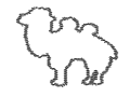
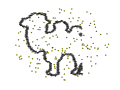
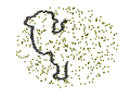
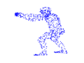
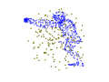
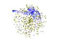
MPO = 0	MPO = 0.2	MPO = 0.5

Figure 4: Examples of 2D and 3D shapes with increasing values of missing point/outliers (mpo). The MPO values used in the experiment ranged from 0 to 0.5.

The number of points in the shapes collected varied between 250 to 10,000 points. This version of the GrassGraph approach focused on equal point-set cardinalities between the source and target shapes. To obtain equal numbers of points, all of the shapes were clustered using the k-means algorithm (using the desired number clusters) where the closest point from the shape to a cluster center was used as the new point. Given the base shape, we now explain how to generate the various noise and MPO artifacts on the shapes.

As mentioned previously, the two standard artifacts that we applied to the clustered shapes were noise and missing points with outliers (MPO). The process of adding noise and MPO artifacts will be referred to as “noise protocol” and “MPO protocol”, respectively. To generate noise in 2D, we uniformly sampled a new point from a circle of radius $r$ around each point. The uniformly sampled point replaced the original point (center of circle) in the shape—the larger the radius of the circle the more noisy the shape became. The same principle applied to 3D shapes, now instead of a circle, we uniformly sampled from a sphere or radius $r$. To generate a noisy shape for experiments, an affine shape was first created, the points are randomly shuffled to remove the correspondence and then the noise protocol is applied.

In the GrassGraph framework, we combine the missing points and outliers into a single artifact. The number of points removed corresponding to the missing point (MP) percentage ($0\leq mp\leq 0.5$) became the same number of points added as outliers. To create outliers, we uniformly draw samples from a circle in 2D and a sphere in 3D of radius $r$ (independent of $r$ for noise generation). To get $r$, the max spread of the points across all coordinate directions was divided by two and multiplied by 1.2. This ensured that the circle or sphere fully encompassed the shape volume, leading to outliers as shown in Figure 4. To generate shapes with MPO for experiments, the artifact was applied to the source shape followed by affine transformation application.

Exp	Dim	#Sh	#NL	#Cases	#Meth	#Aff	#MPO	#Trials
N	2D	20	11	5	4	30	-	132,000
	3D	20	11	5	3	30	-	99,000
MPO	2D	20	-	5	4	30	10	120,000
	3D	20	-	5	3	30	10	90,000
Total Number of Trials								441,000

Table 1: Breakdown of 441,000 experiments used to benchmark the GrassGraph framework. N: Noise; MPO: Missing points with outliers; Dim: Shape dimension; #Sh: No. of base shapes; #NL: No. of noise levels; #Meth: No. of methods; #Aff: No. of affine transformations; #MPO: No. of MPO levels.

To generate affine transformations for 2D and 3D we follow a similar approach taken in [35]. Each transformation is decomposed into a rotation, scale and rotation (in that order) followed by a translation. In 2D, the translation parameters used for the experiments were $\{-30\leq t_{x},t_{y}\leq 30\}$, where $t_{x}$ is the translation in the $x$ direction and $t_{y}$ is the translation in the $y$ direction. The rotation and scale parameters were varied in the following ranges: ${-\pi/2\leq\theta,\sigma\leq\pi/2}$ ,and ${-3\leq s_{x},s_{y}\leq 3}$. Here $\sigma$ is angle of the first 2D rotation matrix, followed by the scaling matrix with $x-$ and $y-$direction parameters $s_{x}$ and $s_{y}$, respectively. The 3D affine transformation matrix is similarly decomposed.

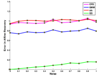
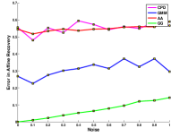
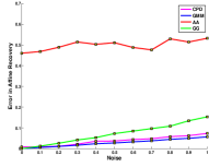
(a) Big-Ang, Big-Sc, No-Trans	(b) Big-Ang, Sm-Sc, Sm-Trans	e) Sm-Ang, Sm-Sc, Sm-Trans
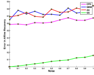
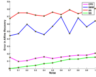
(c) Big-Ang, Med-Sc, Sm-Trans	(d) Med-Ang, Sm-Sc, Sm-Trans

Figure 5: Noise 2D. We outperform the competitors in (a)-(d) as shown above by the green curves and are slightly outperformed in (e) by CPD and GMM. Due to the affine invariance of the proposed GrassGraph (GG) approach, our error curves are consistent across all cases versus the other methods that fluctuate depending on the size of the affine transformation.

	Angle	Scale	Translation
Small	$\pi/6:\pi/6$	$-1:1$	$-10:10$
Medium	$\pi/4:\pi/4$	$-2:2$	$-20:20$
Large	$\pi/2:\pi/2$	$-3:3$	$-30:30$

Table 2: Experimental parameters used to simulate different sizes of affine transformations.

The translations potentially ranged from $\{-30\leq t_{x},t_{y},t_{z}\leq 30\}$, depending on the severity the transformation. The bounds for the three different rotation angles and scale parameters were ${-\pi/2\leq\theta_{x},\theta_{y},\theta_{z},\sigma_{x},\sigma_{y},\sigma_{z}\leq\pi/2}$ and ${-3\leq s_{x},s_{y},s_{z}\leq 3}$. For the experiments, the bounds on the angles, scaling values and translation values were varied to produce different sizes of affine transformations. Table 2 shows the classification of the affine parameters used to simulate the transformations for the experiments.

To perform the experiments, each base shape was transformed with 30 different transformations to form affine shapes. The noise protocol was applied to each of these affine shapes for the eleven values of noise ranging from 0:1 for 2D and 0:5 for 3D. Figure 3 provides examples of noisy shapes in 2D and 3D. All of the affine shapes are evaluated at a single noise level for a particular method—the errors across all the affine shapes are averaged and this error value is assigned to the noise level for that method. For example in Figure 5(a), each marker along a curve represents the average error of the 600 (20 base shapes x 30 affines) affine shapes evaluated at that noise level for the method corresponding to the curve’s color. The results of the noise experiments in 2D and 3D are shown in Figures 5 and 6, respectively. For 2D, across the eleven noise levels with the four methods (GrassGraph and three competitors) we get a total of 132,000 experimental trials and in 3D for the three methods we ran a total of 99,000 trials.

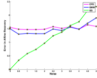
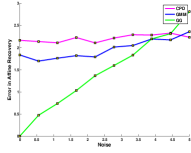
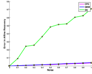
(a) Med-Ang, Sm-Sc, No-Trans	(b) Sm-Ang, Med-Sc, No-Trans	(e) Sm-Ang, Sm-Sc, No-Trans
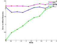
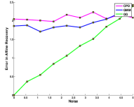
(c) Med-Ang, Med-Sc, No-Trans	(d) Big-Ang, Sm-Sc, No-Trans

Figure 6: Noise 3D. We outperform the competing methods in (a)-(d) at noise levels below 3.5 in (a), 4 in (b), 4.6 in (c) and 4.7 in (d). We trail in (e) in the case of small angles and scale without translation. However, as the sizes of the affines increase, the competing methods are struggle to recover the affine transformation when noise is present whereas our invariant method performs well.

For the 2D noise experiments, the GrassGraph (green) method performed the best across (a)-(d). However, when there was no translation, small angles and small scaling, our method was slightly outperformed by CPD and GMM in (e). Once the affine parameters are increased however, the true utility of our invariant method was highlighted as we outperformed the competing methods. CPD seems to be more susceptible to larger angles and scale whereas GMM is affected more by translations. In case (a), for large affines we see that the competing methods have almost flat curves, this suggests that the correspondences retrieved across all the noise levels are relatively the same, which means that the methods themselves were failing. The Algebraic Affine (AA) method seems to perform the worst across all of the cases, while CPD and GMM fluctuate with the change in affine transformation. Our curve increases gracefully with noise because we are invariant to the affine transformation. We emphasize that only nearest neighbor correspondences were used on the affine invariant coordinates whereas the competing methods required numerical optimization.

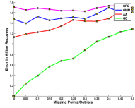
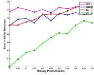
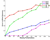
(a) Big-Ang, Med-Sc, Med-Trans	(b) Big-Ang, Med-Sc, Sm-Trans	(e) Sm-Ang, No-Sc, No-Trans
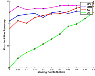
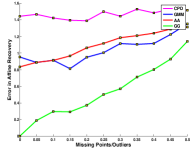
(c) Big-Ang, Big-Sc, No-Trans	(d) Big-Ang, Sm-Sc, No-Trans

Figure 7: MPO 2D. In cases (a)-(d) the GrassGraph approach (green curve) outperforms the competing methods. In case (e) CPD and GMM outperform us but the affine transformation is only a rotation matrix. Once scale and translation are included CPD performs the worst, GMM and AA perform differently depending on the size of the angle and the translation.

In Figure 6, we see that our method outperforms the competing methods at lower noise levels except in case (e) where the affine transformation was very small. The nearest neighbor approach that we employ holds up decently for larger affine transformations versus smaller ones. GMM performs better than CPD in all cases except in (e). The error in our method increases with increasing noise levels due to the affine invariance. This is not the case for the non-affine invariant methods CPD and GMM, which do not fluctuate as much. As we moved up one dimension from 2D to 3D our method still performs well using our simple nearest-neighbor correspondence finding method. This shows that the GrassGraph approach should indeed be the first method considered when recovering correspondences under noisy affine conditions. Now we assess our method’s performance in the presence of missing points and outliers.

The MPO protocol was followed here with the same affine shapes used in the noise experiments, yielding 120,000 trials for 2D and 90,000 for 3D with the results shown in Figures 7 and 8, respectively. In 2D we outperform the competing methods in (a)-(d) and are outperformed by CPD and GMM in (e). Note that the case in (e) has no scale and translation, so it is essentially solving for the rotation. In cases (a)-(d) CPD performs the worst, AA and GMM alternate depending on the scale and translation. When the scale increases between (c) and (d), GMM performs worse than AA. In cases (a) and (b) as the translation changes from small to medium, there is no noticable effect in the competing methods. In 2D, our method proves to be a viable first choice algorithm for correspondence recovery.

Our performance on 3D MPO is somewhat different—the outlier rejection schemes built into the competing methods outperform us in some cases. In cases (a)-(d) we outperform GMM but not CPD. The motion coherence constraint in CPD is able to withstand the increasing outliers and occlusion. As the amount of occlusions and outliers increase, our method has a distinct spike at lower levels and tapers off at higher levels. We attribute this to our simple correspondence finding scheme. In the presence of outliers, the chances of two points being mutual nearest neighbors decreases, hence our error curves flatten out. Although we do not perform better than all the competing methods on 3D MPO, our performance in 2D and 3D still serves as strong evidence that our extremely simple method should be an algorithm of first choice for correspondence recovery.

5 Conclusions

Feature matching is at the heart of many applications in computer vision. Image registration, object recognition, and shape analysis all rely heavily on robust methods for recovery of correspondences and estimation of geometric transformations between domains. As a core need, myriad pioneering efforts and mathematically sophisticated formulations have resulted in a multitude of approaches. However, very few offer the triadic balance of sound theoretical development, ease of implementation, and robust performance as the proposed GrassGraph framework.

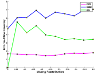
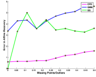
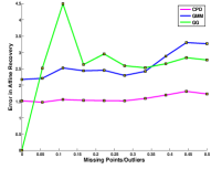
(a) Big-Ang, Sm-Sc, No-Trans	(b) Med-Ang, Sm-Sc, Sm-Trans	(e) Sm-Ang, Sm-Sc, No-Trans
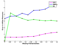
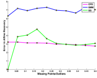
(c) Sm-Ang, Sm-Sc, Sm-Trans	(d) Big-Ang, Sm-Sc, Sm-Trans

Figure 8: MPO 3D. Notice that the GrassGraph approach has a distinct peak at low levels of MPO and it tapers off as the occlusions and outliers increase. This lower performance can be attributed to our simple nearest-neighbor correspondence recovery approach. In cases (a)-(d) we are able to outperform GMM but not CPD because of its coherent motion constraint.

GrassGraph develops a true affine invariant through a two-stage process. First, a Grassmannian representation (GR) is achieved through the use of standard SVD. Secondly, we approximate the Laplace-Beltrami operator (LBO) on the GR domain, whose eigenspace coordinates then free us from an inherent ambiguity present in the coordinates extracted from the GR. Within this true affine invariant setting, establishing correspondences reduces to simple nearest-neighbor selection (though more complex linear assignment solvers can also be used). Correspondences in this new space are bijectively related to the original pair of feature points; hence, we are able to directly recover the affine transformation between them. Our method was evaluated on a broad spectrum of test cases, parameter settings, noise corruption levels, occlusions, and included comparisons to other competing methods. In all, we executed 441,000 experimental trials. Both the number and diversity of test scenarios far exceed other recent efforts. Under such rigorous validation, GrassGraph demonstrated state-of-the-art performance, providing credence to the efficacy of the approach. In the future, we plan to leverage the lessons learned in the present affine matching situation and investigate extensions to the non-rigid case.

References

- [1] D. H. Ballard. Generalized Hough transform to detect arbitrary patterns. IEEE Transactions on Pattern Analysis Machine Intelligence, 13:111–122, 1981.
- [2] E. Begelfor and M. Werman. Affine invariance revisited. In IEEE Conference on Computer Vision and Pattern Recognition, 2006.
- [3] W. M. Boothby. An Introduction to Differentiable Manifolds and Riemannian Geometry. Academic Press, 2002.
- [4] T. Caelli and S. Kosinov. An eigenspace projection clustering method for inexact graph matching. IEEE Transactions on Pattern Analysis and Machine Intelligence, 26:515–519, 2004.
- [5] M. Carcassoni and E. Hancock. Correspondence matching with modal clusters. IEEE Transactions on Pattern Analysis and Machine Intelligence, 25:1609–1615, 2003.
- [6] M. Carcassoni and E. R. Hancock. Spectral correspondence for point pattern matching. Pattern Recognition, 36:193–204, 2003.
- [7] H. Chui and A. Rangarajan. A new point matching algorithm for non-rigid registration. Computer Vision and Image Understanding, 89:114–141, 2003.
- [8] P. Dalal, B. Munsell, S. Wang, J. Tang, K. Oliver, H. Ninomiya, X. Zhou, and H. Fujita. A fast 3D correspondence method for statistical shape modeling. In IEEE Conference on Computer Vision and Pattern Recognition, pages 1–8, 2007.
- [9] C. R. Fan. Spectral Graph Theory. American Mathematical Society, 1997.
- [10] M. A. Fischler and R. A. Elschlager. The representation and matching of pictorial structures. IEEE Transactions on Computers, 22:67–92, 1973.
- [11] V. Ha and J. Moura. Affine-permutation invariance of 2D shapes. IEEE Transactions on Image Processing, 14:1687–1700, 2005.
- [12] J. Ho, M. Yang, A. Rangarajan, and B. Vemuri. A new affine registration algorithm for matching 2D point sets. In IEEE Workshop on Applications of Computer Vision, page 25, 2007.
- [13] J. Isaacs and R. Roberts. Metrics of the Laplace-Beltrami eigenfunctions for 2D shape matching. In IEEE International Conference on Systems, Man and Cybernetics, pages 3347–3352, 2011.
- [14] V. Jain and H. Zhang. Robust 3D shape correspondence in the spectral domain. In IEEE International Conference on Shape Modeling and Applications, pages 19–31, 2006.
- [15] B. Jian and B. C. Vemuri. Robust point set registration using gaussian mixture models. IEEE Transactions on Pattern Analysis and Machine Intelligence, 33:1633–1645, 2011.
- [16] P. W. Jones, M. Maggioni, and R. Schul. Manifold parametrizations by eigenfunctions of the Laplacian and heat kernels. Proceedings of the National Academy of Sciences, 105:1803–1808, 2008.
- [17] Y. Lamdan, J. Schwartz, and H. Wolfson. Affine invariant model-based object recognition. IEEE Transactions on Robotics and Automation, 6:578–589, 1990.
- [18] B. Li, T. Schreck, A. Godil, and et. al. SHREC12 Track: Sketch-Based 3D Shape Retrieval. Eurographics Workshop on 3D Object Retrieval, 2012.
- [19] R. Li, P. Turaga, A. Srivastava, and R. Chellappa. Differential geometric representations and algorithms for some pattern recognition and computer vision problems. Pattern Recognition Letters, 43:3 – 16, 2014.
- [20] B. Luo and E. R. Hancock. Alignment and correspondence using singular value decomposition. In Structural, Syntactic, and Statistical Pattern Recognition, volume 1876, pages 226–235, 2000.
- [21] D. Mateus, F. Cuzzolin, R. Horaud, and E. Boyer. Articulated shape matching using locally linear embedding and orthogonal alignment. In IEEE International Conference on Computer Vision (ICCV), 2007.
- [22] D. Mateus, R. Horaud, D. Knossow, F. Cuzzolin, and E. Boyer. Articulated shape matching using Laplacian eigenfunctions and unsupervised point registration. In IEEE Conference on Computer Vision and Pattern Recognition, 2008.
- [23] M. Moyou, K. E. Ihou, and A. M. Peter. LBO Shape Densities: Efficient 3D shape retrieval using wavelet densities. In IEEE International Conference on Pattern Recognition, 2014.
- [24] A. Myronenko, X. Song, and . Carreira-Perpi n. Non-rigid point set registration: Coherent point drift (CPD). In In Advances in Neural Information Processing Systems 19. MIT Press, 2006.
- [25] A. Peter and A. Rangarajan. The GatorBait 100 shape database. http://www.cise.ufl.edu/~anand/publications.html, 2007.
- [26] D. Raviv, A. M. Bronstein, M. M. Bronstein, D. Waisman, N. A. Sochen, and R. Kimmel. Equi-affine invariant geometry for shape analysis. Journal of Mathematical Imaging and Vision, 50:144–163, 2014.
- [27] M. Reuter, F.-E. Wolter, and N. Peinecke. Laplace-Beltrami spectra as ’Shape-DNA’of surfaces and solids. Computer-Aided Design, 38:342–366, 2006.
- [28] R. M. Rustamov. Laplace-Beltrami eigenfunctions for deformation invariant shape representation. In Proceedings of the fifth Eurographics symposium on Geometry processing, pages 225–233, 2007.
- [29] G. L. Scott and H. C. Longuet-Higgins. An algorithm for associating the features of two images. Proceedings of the Royal Society of London Biological Sciences, 244:21–26, 1991.
- [30] L. S. Shapiro and J. M. Brady. Feature-based correspondence: an eigenvector approach. Image and Vision Computing, 10:283 – 288, 1992.
- [31] K. Siddiqi, A. Shokoufandeh, S. J. Dickinson, and S. W. Zucker. Shock graphs and shape matching. International Journal of Computer Vision, 35:13–32, 1999.
- [32] P. Turaga, A. Veeraraghavan, and R. Chellappa. Statistical analysis on stiefel and grassmann manifolds with applications in computer vision. In IEEE Conference on Computer Vision and Pattern Recognition, pages 1–8, 2008.
- [33] S. Umeyama. An eigendecomposition approach to weighted graph matching problems. IEEE Transactions on Pattern Analysis Machine Intelligence, 10:695–703, 1988.
- [34] Z. Wang and H. Xiao. Dimension-free affine shape matching through subspace invariance. In IEEE Conference on Computer Vision and Pattern Recognition, pages 2482–2487, June 2009.
- [35] J. Zhang and A. Rangarajan. Affine image registration using a new information metric. In IEEE Conference on Computer Vision and Pattern Recognition, pages 848–855, 2004.
- [36] Z. Zhang. Iterative point matching for registration of free-form curves and surfaces. International Journal of Computer Vision, 13:119–152, 1994.
- [37] F. Zhou and F. de la Torre. Factorized graph matching. In IEEE Conference on Computer Vision and Pattern Recognition, pages 127–134, 2012.
- [38] F. Zhou and F. de la Torre. Deformable graph matching. In IEEE Conference on Computer Vision and Pattern Recognition, pages 2922–2929, 2013.