A simple volume-of-fluid reconstruction method for three-dimensional two-phase flows

Abstract

A new PLIC (piecewise linear interface calculation)-type VOF (volume of fluid) method, called APPLIC (approximated PLIC) method, is presented. Although the PLIC method is one of the most accurate VOF methods, the three-dimensional algorithm is complex. Accordingly, it is hard to develop and maintain the computational code. The APPLIC method reduces the complexity using simple approximation formulae. Three numerical tests were performed to compare the accuracy of the SVOF (simplified volume of fluid), VOF/WLIC (weighed line interface calculation), THINC/SW (tangent of hyperbola for interface capturing/slope weighting), THINC/WLIC, PLIC, and APPLIC methods. The results of the tests show that the APPLIC results are as accurate as the PLIC results and are more accurate than the SVOF, VOF/WLIC, THINC/SW, and THINC/WLIC results. It was demonstrated that the APPLIC method is more computationally efficient than the PLIC method.

1 Introduction

Two-phase flows are essential in many research fields; for example, in relation to cloud and precipitation droplets in the atmosphere, water waves, cooling devices, oil and gas pipelines, chemical industrial plants, and thermal power stations. In the recent decades, many interface tracking methods for simulating two-phase flows have been developed. The VOF (volume of fluid) method, originated by Hirt and Nichols [1], is one of the most widely used algorithms. Excellent reviews of the VOF method have been given by Rudman [2], Rider and Kothe [3], Scardovelli and Zaleski [4], and Pilliod and Puckett [5].

The VOF method is based on the spatial discretization of a characteristic function to distinguish between two phases, and the reconstruction of the interfaces for advection. Suppose that we wish to simulate an incompressible two-phase (‘light’ and ‘dark’) flow in the three-dimensional Cartesian space ${\boldsymbol{x}}=(x_{1},x_{2},x_{3})$. The characteristic function for the flow is defined as

$$\chi({\boldsymbol{x}})=\begin{cases}0&\text{if there is light fluid at point ${\boldsymbol{x}}$},\\ 1&\text{if there is dark fluid at point ${\boldsymbol{x}}$}.\end{cases}$$ (1)

The interfaces between the two phases are represented by the discontinuity of the characteristic function. In this paper, we suppose that a computational grid composed of cubic cells of a edge $\Delta x$ is used. Extension of our analysis to general regular grids is straightforward. By descretizing the characteristic function in a computational cell $(i,j,k)$, we can obtain the volume fraction

$$C_{i,j,k} =\frac{1}{(\Delta x)^{3}}\int_{\Omega_{i,j,k}}\chi({\boldsymbol{x}})\,d{\boldsymbol{x}},$$ (2)

where $\Omega_{i,j,k}$ is the domain of the cell. It is obvious from the definition that

$$C_{i,j,k}\begin{cases}=0&\text{if the cell is filled by light fluid},\\ \in(0,1)&\text{if the cell contains both fluids (interface cell)},\\ =1&\text{if the cell is filled by dark fluid}.\end{cases}$$ (3)

The VOF method reconstructs the shape of the interface in each interface cell to evaluate VOF advection fluxes. Various schemes for VOF reconstruction have been presented. The PLIC (piecewise linear interface calculation) method [6, 7] reconstructs an interface in a cell as a plane (in three-dimensional space) or a line (in two-dimensional space) with a given normal vector. The SLIC (simple line interface calculation) method [8] assumes the shape of an interface to be a plane parallel to one of the cell faces. The VOF/WLIC (weighted line interface calculation) method [9] evaluates an advection flux through a cell face as a weighted sum of SLIC fluxes. The SVOF (simplified volume of fluid) method [10] is similar to the VOF/WLIC method, except for the weight formula. In the THINC (tangent of hyperbola for interface capturing) method [11], interfaces are represented by the use of the hyperbolic tangent. Improved THINC methods have also been proposed [9, 12, 13].

Although it is known to be one of the most accurate reconstruction methods, a three-dimensional implementation of the PLIC method is a troublesome task. The PLIC method requires the solution of two geometric problems, as to a cut-volume of a cube by a plane, which are very complicated especially in three-dimensional cases. Scardovelli and Zaleski have provided two sophisticated algorithms (hereafter called the SZ algorithms) to solve these problems [14]. Although the SZ algorithms make the implementation of the PLIC method easier because of their compactness, these are still too complex for quick and easy implementation. Computational routines that implement the SZ algorithms must involve multiple “if” statements, which make it hard to develop and maintain the routines, and potentially inhibit its optimal compilation, especially for processors susceptible to conditional branches, e.g., deeply pipelined processors, processors with SIMD (single instruction multiple data) operations, vector processors, and GPUs (graphics processing units) [15].

In this paper, a PLIC-type VOF method called the APPLIC (approximated PLIC) method is presented. In the APPLIC method, interfaces are reconstructed in a similar manner as in the PLIC method, except that the geometric problems are solved through the use of simple approximation formulae.

This paper is organized as follows. In Section 2, we describe the APPLIC method. Section 3 compares the accuracy and computational efficiency of the APPLIC method with some existing VOF methods. Finally, conclusions are summarized in Section 4.

The following vector notation is used throughout this paper. Bold letters denote three-dimensional vectors and the corresponding non-bold letters with subscripts 1, 2, or 3 denote the vector components. For example, ${\boldsymbol{u}}=(u_{1},u_{2},u_{3})$ and ${\boldsymbol{m}}^{\prime\prime}_{\rm A}=(m^{\prime\prime}_{{\rm A},1},m^{\prime\prime}_{{\rm A},2},m^{\prime\prime}_{{\rm A},3})$. The expression ${\boldsymbol{m}}\geq a$ stands for the condition $m_{1}\geq a$, $m_{2}\geq a$, and $m_{3}\geq a$.

2 Method

2.1 The PLIC method using the SZ algorithms

In this paper, we use directional splitting for advection and a regular staggered grid where velocity components $u_{1}$, $u_{2}$, and $u_{3}$ are stored at the centers of the cell faces $\{(i+1/2,j,k)\}$, $\{(i,j+1/2,k)\}$, and $\{(i,j,k+1/2)\}$, respectively. We assume that the Courant-Friedrichs-Lewy (CFL) condition,

$$\frac{\lvert u_{l}\rvert\Delta t}{\Delta x}<1\quad\text{for all $l\in\{1,2,3\}$},$$ (4)

holds, where $\Delta t$ is the time step size.

Let $\phi$ be the face, and $u_{I}$ ($I=1$, 2, or 3) the velocity component placed on $\phi$. Let $\Omega$ be the donor cell, which is the cell that has $\phi$ as a cell face and lies on the upwind side of $u_{I}$. Let $\phi^{*}$ be the opposite face of the face $\phi$ in the cell $\Omega$. The cell $\Omega$ is partitioned into two subcells by the section $\sigma$ parallel to $\phi$ and laid $\lvert u_{I}\rvert\Delta t$ away from $\phi$. Let $\Omega_{\rm A}$ and $\Omega_{\rm B}$ be the subcells of $\Omega$ between $\phi$ and $\sigma$ and between $\sigma$ and $\phi^{*}$, respectively (see Fig. 1). The section $\sigma$ is always located between $\phi$ and $\phi^{*}$ because of the CFL condition. Let $C_{\rm A}$ and $C_{\rm B}$ be the partial volume fractions in $\Omega_{\rm A}$ and $\Omega_{\rm B}$, respectively, defined as

$$C_{\rm A} =\frac{1}{(\Delta x)^{3}}\int_{\Omega_{\rm A}}\chi({\boldsymbol{x}})\,d{\boldsymbol{x}},$$ (5)

$$C_{\rm B} =\frac{1}{(\Delta x)^{3}}\int_{\Omega_{\rm B}}\chi({\boldsymbol{x}})\,d{\boldsymbol{x}}.$$ (6)

It is obvious that $C_{\rm A}\in[0,1]$ and $C_{\rm B}\in[0,1]$. From the definitions, we have

$$C_{\rm A}+C_{\rm B} =C,$$ (7)

where $C$ is the volume fraction in the donor cell $\Omega$.

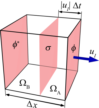
Figure 1: Schematic illustration of a donor cell with respect to a flux through a cell face $\phi$. The cell is divided into two subcells, $\Omega_{\rm A}$ and $\Omega_{\rm B}$, by the section $\sigma$ parallel to $\phi$ and laid $\lvert u_{I}\rvert\Delta t$ away from $\phi$.

The computational advection flux of the volume fraction through the face $\phi$ (i.e., the amount of the volume fraction through the face during $\Delta t$) is obtained via

$$F=C_{\rm A}\operatorname{sgn}u_{I},$$ (8)

where $\operatorname{sgn}$ is the sign function defined as

$$\operatorname{sgn}x =\begin{cases}1&\text{if $x\geq 0$},\\ -1&\text{if $x<0$}.\end{cases}$$ (9)

In some cases, $C_{\rm A}$ is easily determined by

$$C_{\rm A}=\begin{cases}0&\text{if $C=0$ or $\lvert g\rvert=0$},\\ \lvert g\rvert&\text{if $C=1$},\end{cases}$$ (10)

where $\lvert g\rvert$ denote the local CFL number in the cell $\Omega$ with respect to the flux through the face $\phi$:

$$g=\frac{u_{I}\Delta t}{\Delta x}.$$ (11)

Because of the CFL condition, $g$ must be in the range $(-1,1)$. If $C\in(0,1)$ and $\lvert g\rvert>0$, $C_{\rm A}$ is determined through the reconstruction of the interface in the donor cell $\Omega$.

Here, we define the two geometric problems crucial to the PLIC method, which are mutually inverse. Consider a unit cube $U=\{{\boldsymbol{x}}\in[0,1]^{3}\}$ and an oriented plane $P(\alpha,{\boldsymbol{m}})=\{{\boldsymbol{x}}|\,{\boldsymbol{m}}\cdot{\boldsymbol{x}}<\alpha\},$ where ${\boldsymbol{m}}$ is the normal vector of the plane, and $\alpha$ is the plane constant. Note that an oriented plane is not a thin object without volume, but is a solid object with an inside and an outside. Let $V$ be the volume of the intersection between the unit cube and the oriented plane. One of the problems, called the forward problem, is to determine the value of $V$ for given $\alpha$ and ${\boldsymbol{m}}$. The other problem, called the inverse problem, is to determine the value of $\alpha$ for given $V$ and ${\boldsymbol{m}}$. Namely,

$$V(\alpha,{\boldsymbol{m}}) =\int_{U\cap P(\alpha,{\boldsymbol{m}})}d{\boldsymbol{x}},$$ (12)

$$\alpha(V^{\prime},{\boldsymbol{m}}) =\alpha^{\prime}\quad\text{such that\quad$V(\alpha^{\prime},{\boldsymbol{m}})=V^{\prime}$.}$$ (13)

To reduce the complexity of the problems, the SZ algorithms restrict ${\boldsymbol{m}}$ to a vector so that ${\boldsymbol{m}}\geq 0$ and $\|{\boldsymbol{m}}\|_{1}=1$.

The functions $V(\alpha,{\boldsymbol{m}})$ and $\alpha(V,{\boldsymbol{m}})$ have the following properties [4].

1. The value of $V(\alpha,{\boldsymbol{m}})$ is within the range $[0,1]$ and

   $$V(\alpha,{\boldsymbol{m}})=\begin{cases}0&\text{if $\alpha\leq 0$},\\ 1&\text{if $\alpha\geq 1$}.\\ \end{cases}$$ (14)

2. The value of $\alpha(V,{\boldsymbol{m}})$ is within the range $[0,1]$ for $V\in[0,1]$.

3. The functions $V$ and $\alpha$ are invariant with respect to a permutation of $m_{1}$, $m_{2}$, and $m_{3}$.

4. The functions $V$ and $\alpha$ are continuous, one-to-one, and monotonically increasing functions of $\alpha$ and $V$ in the ranges $V\in[0,1]$ and $\alpha\in[0,1]$, respectively.

5. The first derivatives $\partial V/\partial\alpha$ and $\partial\alpha/\partial V$ are continuous and monotonically nondecreasing functions of $\alpha\in(0,1/2]$ and $V\in(0,1/2]$, respectively.

6. The curve $(\alpha,V)$ passes through the points $(0,0)$, $(1/2,1/2)$, and $(1,1)$.

7. If ${\boldsymbol{m}}=(0,0,1)$ and $(0,1/2,1/2)$, the values of $V(\alpha,{\boldsymbol{m}})$ become $\alpha$ and $(2\alpha)^{2}/2$, respectively, for $\alpha\in[0,1/2]$.

8. The curve $(\alpha,V)$ has point symmetry (or odd symmetry) with respect to $(\alpha,V)=(1/2,1/2)$; namely,

   $$V(\alpha,{\boldsymbol{m}}) =1-V(1-\alpha,{\boldsymbol{m}}),$$ (15)

   $$\alpha(V,{\boldsymbol{m}}) =1-\alpha(1-V,{\boldsymbol{m}}).$$ (16)

All the properties except (VII) hold for the arbitrary ${\boldsymbol{m}}$.

Figure 2 shows an example implementation of the SZ algorithms written in Fortran 90. The cbrt function, used in line 44, is an intrinsic function that returns the real cube root of the argument. Although this is not included in the Fortran 90 standard, many Fortran compilers support this. The abs functions in lines and are used to prevent vm2 being negative owing to the numerical error in floating point arithmetic when $\text{vm3}\simeq 1$.

⬇

imodule constants

ii real(8), parameter :: CONST_TINY = 1d-25 ! an extremely small constant

iii real(8), parameter :: CONST_PI = 3.14159265358979323846d0 ! $\pi$

ivend module constants

⬇

1 function calc_v(alpha, vma, vmb, vmc) result(v)

2 ! Preconditions:$\;{\tt vma}\in[0,1],\;{\tt vmb}\in[0,1],\;{\tt vmc}\in[0,1],\;{\tt vma}+{\tt vmb}+{\tt vmc}=1$.

3 use constants

4 real(8), intent(in) :: alpha, vma, vmb, vmc

5 real(8) :: v, a, vm1, vm2, vm3, vm12

6 a = min(alpha, 1d0 - alpha)

7 v = 0d0

8 if (a > 0d0) then

9 vm1 = min(vma, vmb, vmc)       ! Sort $\,{\tt vm1},{\tt vm2},{\tt vm3}$

10 vm3 = max(vma, vmb, vmc)      ! such that $\,{\tt vm1}\leq{\tt vm2}\leq{\tt vm3}\,$.

11 vm2 = abs(1d0 - vm3 - vm1)

12 vm12 = vm1 + vm2

13 if (a < vm1) then

14 v = a ** 3 / (6d0 * vm1 * vm2 * vm3)

15 else if (a < vm2) then

16 v = a * (a - vm1) / (2d0 * vm2 * vm3) + &

17 vm1 ** 2 / (6d0 * vm2 * vm3 + CONST_TINY)

18 else if (a < min(vm12, vm3)) then

19 v = (a ** 2 * (3d0 * vm12 - a) + vm1 ** 2 * (vm1 - 3d0 * a) + &

20 vm2 ** 2 * (vm2 - 3d0 * a)) / (6d0 * vm1 * vm2 * vm3)

21 else if (vm3 < vm12) then

22 v = (a ** 2 * (3d0 - 2d0 * a) + vm1 ** 2 * (vm1 - 3d0 * a) + &

23 vm2 ** 2 * (vm2 - 3d0 * a) + vm3 ** 2 * (vm3 - 3d0 * a)) / &

24 (6d0 * vm1 * vm2 * vm3)

25 else

26 v = (a - 0.5d0 * vm12) / vm3

27 end if

28 end if

29 if (alpha > 0.5d0) v = 1d0 - v

30 end function calc_v

31

32 function calc_alpha(v, vma, vmb, vmc) result(alpha)

33 ! Preconditions:$\;{\tt v}\in(0,1),\;{\tt vma}\in[0,1],\;{\tt vmb}\in[0,1],\;{\tt vmc}\in[0,1],\;{\tt vma}+{\tt vmb}+{\tt vmc}=1$.

34 use constants

35 real(8), intent(in) :: v, vma, vmb, vmc

36 real(8) :: alpha, w, vm1, vm2, vm3, vm12, v1, v3, a0, a1, a2, q0, sp, th

37 w = min(v, 1d0 - v)

38 vm1 = min(vma, vmb, vmc)       ! Sort $\,{\tt vm1},{\tt vm2},{\tt vm3}$

39 vm3 = max(vma, vmb, vmc)      ! such that $\,{\tt vm1}\leq{\tt vm2}\leq{\tt vm3}\,$.

40 vm2 = abs(1d0 - vm3 - vm1)

41 vm12 = vm1 + vm2

42 v1 = vm1 ** 2 / (6d0 * vm2 * vm3 + CONST_TINY)

43 if (w < v1) then

44 alpha = cbrt(6d0 * vm1 * vm2 * vm3 * w)

45 else if (w < v1 + (vm2 - vm1) / (2.0 * vm3)) then

46 alpha = 0.5d0 * (vm1 + sqrt(vm1 ** 2 + 8d0 * vm2 * vm3 * (w - v1)))

47 else

48 alpha = 0d0

49 if (vm3 < vm12) then

50 v3 = (vm3 ** 2 * (3d0 * vm12 - vm3) + vm1 ** 2 * (vm1 - 3d0 * vm3) + &

51 vm2 ** 2 * (vm2 - 3d0 * vm3)) / (6d0 * vm1 * vm2 * vm3)

52 else

53 v3 = 0.5d0 * vm12 / vm3

54 if (v3 <= w) alpha = vm3 * w + 0.5d0 * vm12

55 end if

56 if (alpha == 0.0) then

57 if (w < v3) then

58 a2 = -3d0 * vm12

59 a1 = 3d0 * (vm1 ** 2 + vm2 ** 2)

60 a0 = -(vm1 ** 3 + vm2 ** 3 - 6d0 * vm1 * vm2 * vm3 * w)

61 else

62 a2 = -1.5d0

63 a1 = 1.5d0 * (vm1 ** 2 + vm2 ** 2 + vm3 ** 2)

64 a0 = -0.5d0 * (vm1 ** 3 + vm2 ** 3 + vm3 ** 3 - 6d0 * vm1 * vm2 * vm3 * w)

65 end if

66 q0 = (1d0/6d0) * (a1 * a2 - 3d0 * a0) - a2 ** 3 * (1d0/27d0)

67 sp = sqrt(-1d0/3d0 * a1 + 1d0/9d0 * a2 ** 2)

68 th = 1d0/3d0 * acos(q0 / (sp ** 3))

69 alpha = 2d0 * sp * cos(th + (4d0/3d0 * CONST_PI)) - (1d0/3d0) * a2

70 end if

71 end if

72 if (v > 0.5d0) alpha = 1d0 - alpha

73 end function calc_alpha

Figure 2: Example implementation of the SZ algorithms written in Fortran 90.

the SZ algorithms to evaluate the functions $V(\alpha,{\boldsymbol{m}})$ and $\alpha(V,{\boldsymbol{m}})$, the volume fraction $C_{\rm A}$ for the PLIC method is determined as

$$C_{\rm A}(g,C,{\boldsymbol{n}})=\lvert g\rvert\,V(\alpha^{\prime\prime}_{\rm A},{\boldsymbol{m}}^{\prime\prime}_{\rm A}),$$ (17a)

with

$$\alpha^{\prime\prime}_{\rm A} =\begin{cases}Q^{\prime}_{\rm A}\alpha^{\prime}&\text{if $n_{I}\,g\leq 0$},\\ Q^{\prime}_{\rm A}(\alpha^{\prime}-r_{\rm A})&\text{if $n_{I}\,g>0$},\end{cases}$$ (17b)

$$m^{\prime\prime}_{{\rm A},l} =\begin{cases}Q^{\prime}_{\rm A}m^{\prime}_{l}\lvert g\rvert&\text{if $l=I$},\\ Q^{\prime}_{\rm A}m^{\prime}_{l}&\text{if $l\neq I$},\end{cases}$$ (17c)

$$Q^{\prime}_{\rm A} =\frac{1}{1-r_{\rm A}},$$ (17d)

$$r_{\rm A} =m^{\prime}_{I}(1-\lvert g\rvert),$$ (17e)

$$\alpha^{\prime} =\alpha(C,{\boldsymbol{m}}^{\prime}),$$ (17f)

$$m^{\prime}_{l} =\frac{\lvert n_{l}\rvert}{\|{\boldsymbol{n}}\|_{1}},$$ (17g)

where $l$ is an index running from one to three, and ${\boldsymbol{n}}$ is the normal vector of the interface in the donor cell $\Omega$ oriented from the dark fluid to the light fluid. See Appendix A for the derivation of the equations. The vector ${\boldsymbol{n}}$ is determined as

$${\boldsymbol{n}}=-\nabla C,$$ (18)

where $\nabla C$ is a numerical gradient of the volume fraction. Accurate evaluation of numerical gradients is required for accurate results. Various algorithms to evaluate numerical gradients for the VOF method can be found in the literature [5, 16, 17, 18, 19, 20].

Figure 3 shows an example implementation of the PLIC method written in Fortran 90. Here, the argument vn1 corresponds to $n_{I}$, and vn2 and vn3 correspond to the other components of ${\boldsymbol{n}}$.

⬇

1 function calc_flux_plic(g, c, vn1, vn2, vn3) result(f)

2 ! Preconditions:$\;{\tt g}\in(-1,1),\;{\tt c}\in(0,1).$

3 use constants

4 real(8), intent(in) :: g, c, vn1, vn2, vn3

5 real(8) :: f, absg, alpha, qa, ra, vm1, vm2, vm3

6 absg = abs(g)

7 vm1 = abs(vn1)

8 vm2 = abs(vn2)

9 vm3 = abs(vn3) + CONST_TINY

10 qa = 1d0 / (vm1 + vm2 + vm3)

11 vm1 = vm1 * qa

12 vm2 = vm2 * qa

13 vm3 = vm3 * qa

14 alpha = calc_alpha(c, vm1, vm2, vm3)

15 ra = vm1 * (1d0 - absg)

16 qa = 1d0 / (1d0 - ra)

17 if (g * vn1 > ZERO) alpha = alpha - ra

18 vm1 = vm1 * absg

19 f = calc_v(alpha * qa, vm1 * qa, vm2 * qa, vm3 * qa) * g

20 end function calc_flux_plic

Figure 3: Example implementation of the PLIC algorithm written in Fortran 90.

2.2 Approximation of the forward and the inverse problems

A basic idea of the APPLIC method is to evaluate $V(\alpha,{\boldsymbol{m}})$ and $\alpha(V,{\boldsymbol{m}})$ by use of simple approximation formulae. In the APPLIC method, the function $V(\alpha,{\boldsymbol{m}})$ for $\alpha\in[0,1/2]$ is approximated as

$$\widetilde{V}(\alpha,{\boldsymbol{m}}) =\frac{1}{2}(2\alpha)^{p},$$ (19)

where $p$ is a positive-valued function of ${\boldsymbol{m}}$. The approximation of the function $\alpha(V,{\boldsymbol{m}})$ for $V\in[0,1/2]$ is derived by solving Eq. (19) for $\alpha$:

$$\widetilde{\alpha}(V,{\boldsymbol{m}}) =\frac{1}{2}(2V)^{1/p}.$$ (20)

Here a tilde ($\;\widetilde{\mbox{}}\;$) indicates an approximation. Using Eqs. (16) and (20), we can give the formula of $\widetilde{\alpha}$ for $V\in[0,1]$ as

$$\widetilde{\alpha}(V,{\boldsymbol{m}}) =\begin{cases}\dfrac{1}{2}(2V)^{p}&\text{if $V\leq 1/2$},\\ 1-\dfrac{1}{2}[2(1-V)]^{p}&\text{if $V>1/2$}.\end{cases}$$ (21)

Similarly, using Eqs. (14), (15), and (19), we have

$$\widetilde{V}(\alpha,{\boldsymbol{m}}) =\begin{cases}0&\text{if $\alpha\leq 0$},\\ \dfrac{1}{2}(2\alpha)^{p}&\text{if $0<\alpha\leq 1/2$},\\ 1-\dfrac{1}{2}[2(1-\alpha)]^{p}&\text{if $1/2<\alpha<1$},\\ 1&\text{if $\alpha\geq 1$}.\end{cases}$$ (22)

The functions $\widetilde{V}$ and $\widetilde{\alpha}$ satisfy properties (I), (II), (IV), (V), (VI), and (VIII).

Let us formulate the function $p$. First, we determine the optimal $p$, denoted by $p_{\rm opt}$, that minimizes the square error $D$, defined as

$$D=\int_{0}^{\frac{1}{2}}[\widetilde{V}(\alpha,{\boldsymbol{m}})-V(\alpha,{\boldsymbol{m}})]^{2}d\alpha+\int_{0}^{\frac{1}{2}}[\widetilde{\alpha}(V,{\boldsymbol{m}})-\alpha(V,{\boldsymbol{m}})]^{2}dV.$$ (23)

The function $p_{\rm opt}$ is plotted in Fig. 4.

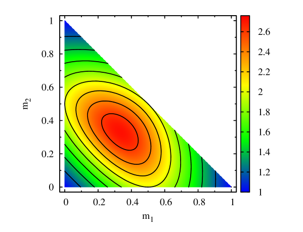
Figure 4: Plot for $p_{\rm opt}$ as a function of ${\boldsymbol{m}}$. The component $m_{3}$ is given by $1-m_{1}-m_{2}$. The contour lines are drawn at $p_{\rm opt}=1$, 1.2, 1.4, $\ldots$, 2.6.

Next, we construct an arithmetic expression of $p$ that approximates $p_{\rm opt}$. We found that $p_{\rm opt}$ can be approximated as

$$p =\frac{c_{2}\xi^{2}+c_{1}\xi+c_{0}}{\xi+c_{0}},$$ (24)

with

$$\xi =(b-m_{1})(b-m_{2})(b-m_{3})-a,$$ (25)

where $c_{0}$, $c_{1}$, $c_{2}$, $a$, and $b$ are constants. To satisfy property (III), Eq. (25) is designed to be symmetric with respect to $m_{1}$, $m_{2}$, and $m_{3}$. We the following relations to satisfy property (VII):

$$c_{0} =\frac{b}{16}(c_{2}b+4c_{1}-8),$$ (26)

$$a =b^{2}(b-1).$$ (27)

The optimal values of $b$, $c1$, and $c2$, shown in Table 1, were determined by a least-square procedure that minimizes the mean square error $\bar{D}$ with respect to ${\boldsymbol{m}}$, defined as

$$\bar{D}=\frac{\displaystyle\iint_{S_{1}}D\left(\frac{{\boldsymbol{n}}}{\|{\boldsymbol{n}}\|_{1}}\right)dS}{\displaystyle\iint_{S_{1}}dS},$$ (28)

where $S_{1}$ is the part of the unit spherical surface in the first octant, namely,

$$S_{1} =\{{\boldsymbol{x}}\,|\,\text{${\boldsymbol{x}}\geq 0$ and $\|{\boldsymbol{x}}\|_{2}=1$}\},$$ (29)

${\boldsymbol{n}}$ is a vector that scans $S_{1}$, and $dS$ is the surface element. Figure 5 shows $p$ given by Eq. (24) with the optimal $b$, $c_{1}$, and $c_{2}$. Here, $p_{\rm opt}$ is also plotted for comparison, denoted by white and dotted contour lines. The function $p$ given by Eq. (24) fits with $p_{\rm opt}$ extremely well.

Table 1: Optimal values of the constants

$b$
$c_{1}$
$c_{2}$

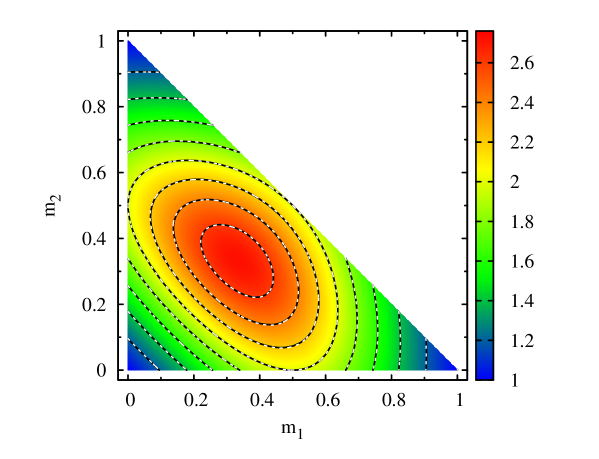
Figure 5: Plot for $p$ (the color image and the black solid contour lines), as obtained by Eq. (24) as a function of ${\boldsymbol{m}}$. The component $m_{3}$ is given by $1-m_{1}-m_{2}$. The contour lines for $p_{\rm opt}$ are also shown as white dotted lines for comparison. The contour lines are drawn at $p=1$, 1.2, 1.4, $\ldots$, 2.6.

The square error $D$ for $p$ obtained by Eq. (24) is plotted in Fig. 6. This figure shows that $D$ becomes the maximum, $D_{\rm max}=2.70\times 10^{-4}$, at ${\boldsymbol{m}}=(0.734,0.133,0.133)$, $(0.133,0.734,0.133)$, and $(0.133,0.133,0.734)$, and becomes zero at ${\boldsymbol{m}}=(1,0,0)$, $(0,1,0)$, $(0,0,1)$, $(0,1/2,1/2)$, $(1/2,0,1/2)$, and $(1/2,1/2,0)$. In Fig. 7, we show $V$ and $\widetilde{V}$ as functions of $\alpha$ for various orientations of ${\boldsymbol{m}}$. In each pane, curves $V(\alpha,{\boldsymbol{m}})$ and $\widetilde{V}(\alpha,{\boldsymbol{m}})$ are plotted for a specific ${\boldsymbol{m}}$. This figure shows that the discrepancy between $V$ and $\widetilde{V}$ is sufficiently small for any ${\boldsymbol{m}}$. Panel (q) indicates the case of ${\boldsymbol{m}}=(0.125,0.125,0,75)$, which has the largest square error ($D=2.68\times 10^{-4}$) among the cases plotted in Fig. 7. Note that $(0.125,0.125,0,75)$ is close to $(0.133,0.133,0.734)$, a case with the maximum square error.

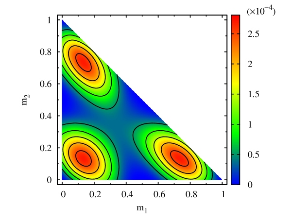
Figure 6: Plot for the square error defined as Eq. (23) as a function of ${\boldsymbol{m}}$. The component $m_{3}$ is given by $1-m_{1}-m_{2}$. The contour lines are drawn at $D=0.5\times 10^{-4}$, $1.0\times 10^{-4}$, $1.5\times 10^{-4}$, $\ldots$, $2.5\times 10^{-4}$.

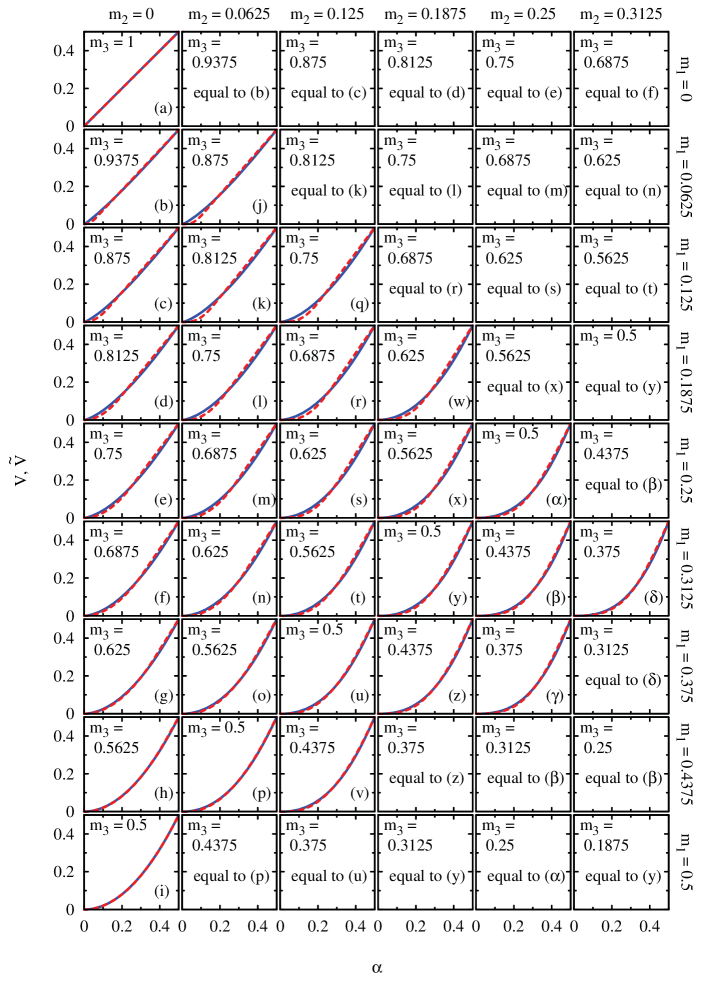
Figure 7: Comparison between the functions $V(\alpha,{\boldsymbol{m}})$ () and $\widetilde{V}(\alpha,{\boldsymbol{m}})$ () as functions of $\alpha$ for various ${\boldsymbol{m}}$.

Figure 8 shows an example implementation of the functions $\widetilde{V}$ and $\widetilde{\alpha}$ written in Fortran 90. In lines and , the expression $\exp(\log(A)*B)$ is used instead of the expression $A\,\mbox{$*\!*$}\,B$. Both the expressions are mathematically equivalent if both $A$ and $B$ are positive. Note that the variables a, p, and invp in Fig. 8 are always positive. However, the former expression requires slightly less computational cost then the latter expression in most computer environments because the evaluation of $A\,\mbox{$*\!*$}\,B$ internally involves multiple conditional branches, e.g., if $A$ is positive/negative, if $B$ is positive/negative, and if $B$ is . If C/C++ is used, the expression ${\rm exp2}({\rm log2}(A)*B)$ may slightly more efficient.

⬇

imodule applic_constants

ii real(8), parameter :: PB = 1.49d0, PC2 = 0.239d0, PC1 = 0.132d0, &

iii PC0 = (PB * (PB * PC2 + 4d0 * PC1 - 8d0) / 16d0), &

iv PA = (PB * PB * (PB - 1d0))

vend module applic_constants

⬇

1 function calc_approx_v(alpha, vma, vmb, vmc) result(v)

2 ! Preconditions:$\;{\tt vma}\in[0,1],\;{\tt vmb}\in[0,1],{\tt vmc}\in[0,1],\;{\tt vma}+{\tt vmb}+{\tt vmc}=1$.

3 use applic_constants

4 real(8), intent(in) :: alpha, vma, vmb, vmc

5 real(8) :: v, a, xi, p

6 a = min(alpha, 1d0 - alpha)

7 v = 0d0

8 if (a > 0d0) then

9 xi = (PB - vma) * (PB - vmb) * (PB - vmc) - PA

10 p = ((PC2 * xi + PC1) * xi + PC0) / (xi + PC0)

11 v = 0.5d0 * exp(log(a + a) * p)

12 end if

13 if (alpha > 0.5d0) v = 1d0 - v

14 end function calc_approx_v

15

16 function calc_approx_alpha(v, vma, vmb, vmc) result(alpha)

17 ! Preconditions:$\;{\tt v}\in(0,1),\;{\tt vma}\in[0,1],\;{\tt vmb}\in[0,1],\;{\tt vmc}\in[0,1],\;{\tt vma}+{\tt vmb}+{\tt vmc}=1$.

18 use applic_constants

19 real(8), intent(in) :: v, vma, vmb, vmc

20 real(8) :: alpha, w, xi, invp

21 w = min(v, ONE - v)

22 xi = (PB - vma) * (PB - vmb) * (PB - vmc) - PA

23 invp = (xi + PC0) / ((PC2 * xi + PC1) * xi + PC0)

24 alpha = 0.5d0 * exp(log(w + w) * invp)

25 if (v > 0.5d0) alpha = 1d0 - alpha

26 end function calc_approx_alpha

Figure 8: Example implementation of the approximation functions $\widetilde{V}$ and $\widetilde{\alpha}$ written in Fortran 90.

2.3 The crude APPLIC method

Using the approximation functions $\widetilde{V}(\alpha,{\boldsymbol{m}})$ and $\widetilde{\alpha}(V,{\boldsymbol{m}})$ instead of functions ${V}(\alpha,{\boldsymbol{m}})$ and ${\alpha}(V,{\boldsymbol{m}})$ in Eq. (17), we can determine computational advection fluxes via Eq. (8). This straightforward method is called the crude APPLIC method.

The crude APPLIC method is not practical because of a defects described below. Let us examine whether fluxes evaluated by the crude APPLIC method have properties which are essential to be satisfied by fluxes of volume fractions. The computational advection flux $F$ should satisfy the followings conditions:

$$F(g,C,{\boldsymbol{n}}) \begin{cases}\geq 0&\text{if $g>0$,}\\ =0&\text{if $g=0$,}\\ \leq 0&\text{if $g<0$,}\end{cases}$$ (30)

$$F[g,C,(n_{1},n_{2},n_{3})] =s_{I}F[s_{I}g,C,(s_{1}n_{1},s_{2}n_{2},s_{3}n_{3})],$$ (31)

$$F[g,C,(n_{1},n_{2},n_{3})] =F[g,C,(n_{1},n_{3},n_{2})],$$ (32)

$$g =F(g,C,{\boldsymbol{n}})+F(g,1-C,-{\boldsymbol{n}}),$$ (33)

$$\lvert F(g,C,{\boldsymbol{n}})\rvert \leq C,$$ (34)

where $s_{i}$ in Eq. (31) is either $1$ or $-1$. In Eq. (32) we suppose that $I=1$ for simplicity. Condition (30) specifies the sign of $F$. Condition (31) from the symmetry of positive and negative directions along the coordinate axes. Conditions (32) from the permutation symmetry between the second- and the third-coordinate axes. As shown in (a) and (b) of Fig. 9, the second term in the right-hand side of Eq. (33) corresponds to the flux of the light fluid. Therefore, condition (33) means that the total flux, given by $g$, is the sum of the light fluid flux and the dark fluid flux. Condition (34) provides the upper limit of $\lvert F\rvert$ under the CFL condition.

A lower limit of $\lvert F\rvert$ is derived from Eqs. (30), (33) and (34) as follows. From Eqs. (30) and (33), we have

$$\lvert F(g,C,{\boldsymbol{n}})\rvert+\lvert F(g,1-C,{\boldsymbol{n}})\rvert =\lvert g\rvert,$$

$$\lvert F(g,1-C,{\boldsymbol{n}})\rvert \leq 1-C.$$ (35)

These leads

$$\lvert F(g,C,n)\rvert\geq\lvert g\rvert-(1-C).$$ (36)

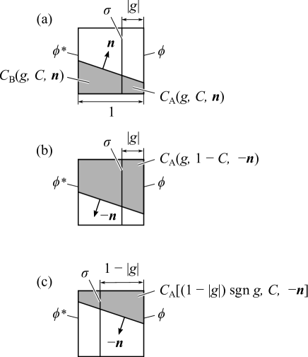
Figure 9: Two-dimensional schematic of the relation among partial volume fractions in a donor cell. The sides of the cells are scaled to be unity.

Although conditions (30), (31), (32), and (33) are always satisfied by the crude APPLIC method, conditions (34) not. To demonstrate this, a set of sample points, ${S}=\{(g^{(l)},C^{(l)},{\boldsymbol{n}}^{(l)})\,|\,l=1,2,\ldots,N\}$ $(N=10,000,000)$, is used. The sample points in the set $S$ were generated such that $\{g^{(l)}\}$, $\{C^{(l)}\}$, and $\{{\boldsymbol{n}}^{(l)}\}$ are uniformly distributed on $[0,1]$, $[0,1]$, and the unit spherical surface, respectively, by use of pseudorandom numbers. Among the sample points in the set $S$, % of the points do not satisfy the condition , where $\widetilde{F}_{\rm CAPPLIC}$ is a flux obtained by the crude APPLIC method. An easy remedy for the defect is to adopt the limiter as follows:

$$\widetilde{F}_{\rm CAPPLIC/L}=\min\{C,\max[\lvert\widetilde{F}_{\rm CAPPLIC}\rvert,\lvert g\rvert-(1-C)]\}\operatorname{sgn}g,$$ (37)

where $\widetilde{F}_{\rm CAPPLIC/L}$ is a flux obtained by the crude APPLIC method with the limiter.

2.4 The APPLIC method

Consider the following relation:

$$\widetilde{C}_{{\rm A}}+\widetilde{C}_{{\rm B}} =C,$$ (38)

where $\widetilde{C}_{{\rm B}}$ is

$$\widetilde{C}_{{\rm B}}(g,C,{\boldsymbol{n}}) =\widetilde{C}_{{\rm A}}[(1-\lvert g\rvert)\operatorname{sgn}g,C,-{\boldsymbol{n}}].$$ (39)

See (a) and (c) of Fig. 9 for a geometric interpretation of Eq. (39). Equation (38) is identical to Eq. (7) except that ${C}_{{\rm A}}$ and ${C}_{{\rm B}}$ are obtained by use of the approximation functions $\widetilde{V}$ and $\widetilde{\alpha}$. Generally, Eq. (38) does not hold because of approximation errors in $\widetilde{V}$ and $\widetilde{\alpha}$.

To improve the crude APPLIC method, we take advantage of the defect that Eq. (38) does not hold. There are two ways to calculate $F$ by use of $\widetilde{V}$ and $\widetilde{\alpha}$:

$$\widetilde{F}_{\rm A}(g,C,{\boldsymbol{n}}) =\widetilde{C}_{\rm A}(g,C,{\boldsymbol{n}})\operatorname{sgn}g,$$ (40)

$$\widetilde{F}_{\rm B}(g,C,{\boldsymbol{n}}) =[C-\widetilde{C}_{\rm B}(g,C,{\boldsymbol{n}})]\operatorname{sgn}g.$$ (41)

In general, $\widetilde{F}_{\rm A}$ and $\widetilde{F}_{\rm B}$ are close but not equal. The crude APPLIC method uses only Eq. (40) to evaluate flux (i.e., $\widetilde{F}_{\rm CAPPLIC}$ is identical to $\widetilde{F}_{\rm A}$), whereas the APPLIC method uses either $\widetilde{F}_{\rm A}$ or $\widetilde{F}_{\rm B}$ as follows:

$$\widetilde{F}_{\rm APPLIC}(g,C,{\boldsymbol{n}}) =\begin{cases}\widetilde{F}_{\rm A}(g,C,{\boldsymbol{n}})&\text{if $\operatorname{pred}(g,C,{\boldsymbol{n}})$ is true},\\ \widetilde{F}_{\rm B}(g,C,{\boldsymbol{n}})&\text{otherwise}.\end{cases}$$ (42)

where $\operatorname{pred}$ is a choice criterion, which is a logical (or Boolean-valued) function that returns either a true or false value. The ideal (i.e., impractical) criterion returns true if $\lvert\widetilde{F}_{\rm A}(g,C,{\boldsymbol{n}})-F_{\rm PLIC}(g,C,{\boldsymbol{n}})\rvert$ is smaller than $\lvert\widetilde{F}_{\rm B}(g,C,{\boldsymbol{n}})-F_{\rm PLIC}(g,C,{\boldsymbol{n}})\rvert$ and false otherwise, where $F_{\rm PLIC}$ denotes the flux obtained by the PLIC method.

Using Eq. (17), we have

$$\widetilde{C}_{\rm A}(g,C,{\boldsymbol{n}}) =\lvert g\rvert\,\widetilde{V}(\widetilde{\alpha}^{\prime\prime}_{\rm A},{\boldsymbol{m}}^{\prime\prime}_{\rm A}),$$ (43a)

$$\widetilde{C}_{\rm B}(g,C,{\boldsymbol{n}}) =(1-\lvert g\rvert)\,\widetilde{V}(\widetilde{\alpha}^{\prime\prime}_{\rm B},{\boldsymbol{m}}^{\prime\prime}_{\rm B}),$$ (43b)

with

$$\widetilde{\alpha}^{\prime\prime}_{\rm A} =\begin{cases}Q^{\prime}_{\rm A}\widetilde{\alpha}^{\prime}&\text{if $n_{I}\,g\leq 0$},\\ Q^{\prime}_{\rm A}(\widetilde{\alpha}^{\prime}-r_{\rm A})&\text{if $n_{I}\,g>0$},\end{cases}$$ (43c)

$$\widetilde{\alpha}^{\prime\prime}_{\rm B} =\begin{cases}Q^{\prime}_{\rm B}(\widetilde{\alpha}^{\prime}-r_{\rm B})&\text{if $n_{I}\,g\leq 0$},\\ Q^{\prime}_{\rm B}\widetilde{\alpha}^{\prime}&\text{if $n_{I}\,g>0$},\end{cases}$$ (43d)

$$m^{\prime\prime}_{{\rm B},l} =\begin{cases}Q^{\prime}_{\rm B}m^{\prime}_{l}(1-\lvert g\rvert)&\text{if $l=I$},\\ Q^{\prime}_{\rm B}m^{\prime}_{l}&\text{if $l\neq I$},\end{cases}$$ (43e)

$$Q^{\prime}_{\rm B} =\frac{1}{1-r_{\rm B}},$$ (43f)

$$r_{\rm B} =m^{\prime}_{I}\,\lvert g\rvert,$$ (43g)

$$\widetilde{\alpha}^{\prime} =\widetilde{\alpha}(C,{\boldsymbol{m}}).$$ (43h)

The author proposes the following choice criterion for the APPLIC method: true if $\lvert\widetilde{\alpha}^{\prime\prime}_{\rm A}-1/2\rvert>\lvert\widetilde{\alpha}^{\prime\prime}_{\rm B}-1/2\rvert$ and false otherwise. See Appendix B for the derivation of the choice criterion. Figure 10 shows an example implementation of the APPLIC method with the proposed criterion written in Fortran 90.

⬇

1 function calc_flux_applic(g, c, vn1, vn2, vn3) result(f)

2 ! Preconditions:$\;{\tt g}\in(-1,1),\;{\tt c}\in(0,1).$

3 use constants

4 real(8), intent(in) :: g, c, vn1, vn2, vn3

5 real(8) :: f, absg, alpha, alphb, ra, rb, qa, qb, vm1, vm2, vm3, v, sw

6 absg = abs(g)

7 vm1 = abs(vn1)

8 vm2 = abs(vn2)

9 vm3 = abs(vn3) + CONST_TINY

10 qa = 1d0 / (vm1 + vm2 + vm3)

11 vm1 = vm1 * qa

12 vm2 = vm2 * qa

13 vm3 = vm3 * qa

14 alpha = calc_approx_alpha(c, vm1, vm2, vm3)

15 rb = vm1 * absg

16 ra = vm1 - rb

17 qb = 1d0 / (1d0 - rb)

18 qa = 1d0 / (1d0 - ra)

19 alphb = (alpha - merge(0d0, rb, vn1 * g > 0d0)) * qb

20 alpha = (alpha - merge(ra, 0d0, vn1 * g > 0d0)) * qa

21 sw = 0d0

22 if (abs(alphb - 0.5d0) > abs(alpha - 0.5d0)) then

23 sw = 1d0

24 alpha = alphb

25 qa = qb

26 rb = ra

27 end if

28 v = calc_approx_v(alpha, rb * qa, vm2 * qa, vm3 * qa)

29 f = sign((c - v) * sw + v * absg, g)

30 end function calc_flux_applic

Figure 10: Example implementation of the APPLIC method with the proposed criterion written in Fortran 90.

Now the approximation accuracy of fluxes obtained by the APPLIC method is examined. Table 2 compares the statistics for the approximation errors of the crude APPLIC method, crude APPLIC method with Eq. (37) as a limiter, APPLIC method, and APPLIC method with the ideal criterion, for the point set $S$. Here, the approximation errors of a flux is defined as the difference between the flux and that obtained by the PLIC method. It is observed that applying the limiter to the crude APPLIC method reduces the mean error . The last row is for the APPLIC method with the ideal criterion, and indicates the lower limits for the mean errors and the maximum errors for any choice criteria.

Table 2: Statistics of the approximation errors of fluxes for the point set $S$.

Method	Correct answer ratea	Mean errorb	Maximum errorc
Crude APPLIC	50.0%	$2.89\times 10^{-3}$	$\times 10^{-2}$
Crude APPLIC with limiter	—	$\times 10^{-3}$	$\times 10^{-2}$
APPLIC	71.5%	$1.88\times 10^{-3}$	$\times 10^{-2}$
APPLIC with ideal criterion	100%	$1.43\times 10^{-3}$	$\times 10^{-2}$
$\!\!\!{}^{\rm a}$The percentage of the sample points where the criterion provides true if $\lvert\widetilde{F}_{{\rm A}}-F_{\rm PLIC}\rvert<\lvert\widetilde{F}_{{\rm B}}-F_{\rm PLIC}\rvert$ and false otherwise.
$\!\!\!{}^{\rm b}$The arithmetic mean of the absolute errors.
$\!\!\!{}^{\rm c}$The maximum value of the absolute errors.

Figures 11 and 12 show the dependence of approximation errors of fluxes on $\lvert g\rvert$ and $C$. The errors in the figures were evaluated by using 50000 three-dimensional vectors distributed uniformly on the unit spherical surface as sample points of ${\boldsymbol{n}}$. All the plots are axisymmetric with respect to $C=0.5$ since the PLIC, crude APPLIC, crude APPLIC with limiter, APPLIC, and APPLIC with ideal criterion satisfy Eq. (33). Moreover, the plots for the APPLIC and the APPLIC with ideal criterion are axisymmetric with respect to $\lvert g\rvert=0.5$ since the PLIC, APPLIC, and APPLIC with ideal criterion satisfy that $F_{{\rm A}}$ equals to $F_{{\rm B}}$.

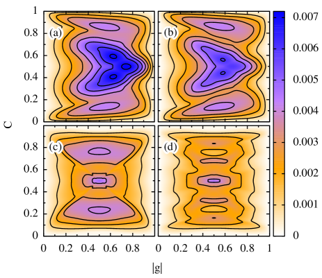
Figure 11:

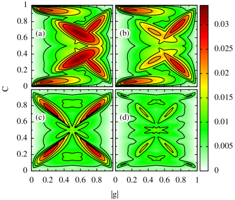
Figure 12:

The APPLIC method satisfies conditions (34) as well as conditions (30)-(33). Moreover, the following condition tighter than conditions (30), (34) is also satisfied:

$$F\in[{\rm LB},{\rm UB}],$$ (44)

with

$${\rm LB} =\begin{cases}gC&\text{if $n_{I}\leq 0$,}\\ \max[g-(1-C),0]&\text{if $n_{I}>0$ and $g\geq 0$,}\\ \max[g,-C]&\text{if $n_{I}>0$ and $g<0$,}\end{cases}$$ (45)

$${\rm UB} =\begin{cases}gC&\text{if $n_{I}\geq 0$,}\\ \min[g+(1-C),0]&\text{if $n_{I}<0$ and $g\leq 0$,}\\ \min[g,C]&\text{if $n_{I}<0$ and $g>0$.}\end{cases}$$ (46)

These bounds are derived from fluxes for SLIC-type fluid configurations [10].

We now demonstrate that the APPLIC method satisfies condition (44) using the set $S$. Among the sample points in the set $S$, 5.6% of the points do not satisfy the relation $\widetilde{F}_{\rm A}\in[{\rm LB},{\rm UB}]$. Similarly, 5.6% of the points do not satisfy $\widetilde{F}_{\rm B}\in[{\rm LB},{\rm UB}]$. However, all the points meet either $\widetilde{F}_{\rm A}\in[{\rm LB},{\rm UB}]$ or $\widetilde{F}_{\rm B}\in[{\rm LB},{\rm UB}]$.

Figure 13 depicts the points in the set $S$ such that ${\widetilde{F}_{\rm A}}\notin[{\rm LB},{\rm UB}]$ (blue dots) and ${\widetilde{F}_{\rm B}}\notin[{\rm LB},{\rm UB}]$ (red dots). Each dot is placed at $(\lvert\widetilde{\alpha}^{\prime\prime}_{\rm A}-1/2\rvert,\,\lvert\widetilde{\alpha}^{\prime\prime}_{\rm B}-1/2\rvert)$ on the plot. All the blue and the red dots lie in the regions $\lvert\widetilde{\alpha}^{\prime\prime}_{\rm A}-1/2\rvert<\lvert\widetilde{\alpha}^{\prime\prime}_{\rm B}-1/2\rvert$ and $\lvert\widetilde{\alpha}^{\prime\prime}_{\rm A}-1/2\rvert>\lvert\widetilde{\alpha}^{\prime\prime}_{\rm B}-1/2\rvert$, respectively. This indicates that fluxes evaluated by the APPLIC method with the proposed choice criterion always satisfy Eq. (44).

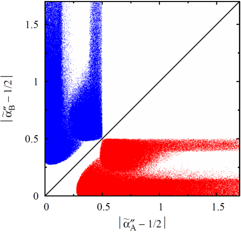
Figure 13: The sample points in the set $S$ so that ${\widetilde{F}_{\rm A}}\notin[\rm LB,UB]$ (blue dots) and ${\widetilde{F}_{\rm B}}\notin[\rm LB,UB]$ (red dots). The solid line represents the line $\lvert\widetilde{\alpha}^{\prime\prime}_{\rm A}-1/2\rvert=\lvert\widetilde{\alpha}^{\prime\prime}_{\rm B}-1/2\rvert$.

3 Numerical tests

3.1 The accuracy of advection

We compare the accuracy of advection for the APPLIC method with other VOF methods over three test problems. The VOF methods examined in this section are as follows: SVOF, VOF/WLIC, THINC/SW, THINC/WLIC, PLIC, and APPLIC. Each test problem is designed so that the initial distribution (at $t=0$) of the light and dark fluids is theoretically identical with the final distribution. The $L_{1}$ error, defined as ${\sum_{i,j,k}(\Delta x)^{3}\left\lvert C_{i,j,k}(t=0)-C_{i,j,k}(t=T)\right\rvert}$, is employed to compare the accuracy, where $T$ is the final time. Parker and Youngs’ method [16, 21] is adopted to evaluate surface normals. We adopt an operator splitting algorithm for the advection of volume fractions as follows:

$$C_{i,j,k}^{*} =C_{i,j,k}^{(n)}-F_{i+\frac{1}{2},j,k}^{(n)}+F_{i-\frac{1}{2},j,k}^{(n)}+\frac{C_{i,j,k}^{(n)}\Delta t}{\Delta x}(u_{1:i+\frac{1}{2},j,k}-u_{1:i-\frac{1}{2},j,k}),$$ (47a)

$$C_{i,j,k}^{**} =C_{i,j,k}^{*}-F_{i,j+\frac{1}{2},k}^{*}+F_{i,j-\frac{1}{2},k}^{*}+\frac{C_{i,j,k}^{(n)}\Delta t}{\Delta x}(u_{2:i,j+\frac{1}{2},k}-u_{2:i,j-\frac{1}{2},k}),$$ (47b)

$$C_{i,j,k}^{(n+1)} =C_{i,j,k}^{**}-F_{i,j,k+\frac{1}{2}}^{**}+F_{i,j,k-\frac{1}{2}}^{**}+\frac{C_{i,j,k}^{(n)}\Delta t}{\Delta x}(u_{3:i,j,k+\frac{1}{2}}-u_{3:i,j,k-\frac{1}{2}}),$$ (47c)

where the superscript $(n)$ refers to the temporal indices, and the superscripts $*$ and $**$ represent quantities at the first and second intermediate steps, respectively. The order of directions of Eq. (47) is changed at each time step to minimize possible asymmetries. All floating point arithmetic is done in double-precision.

3.1.1

In the first test problem, a shape defined as the union of the rectangular parallelepipeds $\{{\boldsymbol{x}}\in[0.08,0.48]\times[0.2,0.36]\times[0.2,0.36]\}$ and the sphere with center $(0.28,0.28,0.28)$ and radius $0.15$ is translated in a computational domain $[0,1]\times[0,1]\times[0,1]$. We set the final time as $T=0.8$. The shape $B$ is advected in the following uniform velocity field:

$${\boldsymbol{u}}=\begin{cases}(1,1,1)&\text{if $t<T/2$},\\ (-1,-1,-1)&\text{if $t>T/2$}.\end{cases}$$ (48)

Figure 14 compares the initial shape and the final shapes using a $100\times 100\times 100$ ($\Delta x=0.01$) grid with $\Delta t=0.005$, where the CFL number is 0.5. The THINC/SW method produces significantly deformed shape. Table 3 presents the $L_{1}$ errors and the corresponding convergence rate for $25\times 25\times 25$ $(\Delta x=0.04)$, $50\times 50\times 50$ $(\Delta x=0.02)$, and $100\times 100\times 100$ $(\Delta x=0.01)$, grids, where $\Delta t=0.02$, 0.001, and 0.005, respectively.

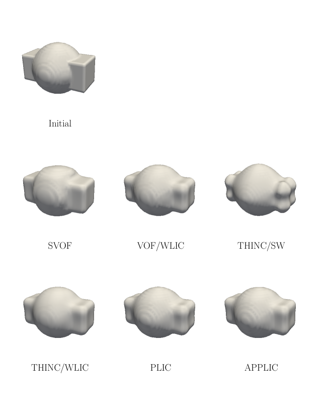
Figure 14: The initial $(t=0)$ and the final $(t=T)$ shapes for test 1, using a 100$\times$100$\times$100 grid with $\Delta t=0.005$.

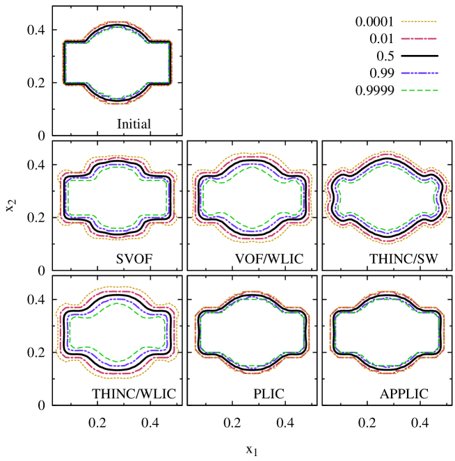
Figure 15:

Table 3: $L_{1}$ errors and convergence rates using different grid sizes for test 1.

Method	$25\times 25\times 25$	Rate	$50\times 50\times 50$	Rate	$100\times 100\times 100$
SVOF	$4.19\times 10^{-3}$	0.74	$2.50\times 10^{-3}$	1.03	$1.22\times 10^{-3}$
VOF/WLIC	$3.77\times 10^{-3}$	0.84	$2.11\times 10^{-3}$	1.23	$8.99\times 10^{-4}$
THINC/SW	$3.35\times 10^{-3}$	0.46	$2.44\times 10^{-3}$	1.03	$1.19\times 10^{-3}$
THINC/WLIC	$4.57\times 10^{-3}$	0.86	$2.51\times 10^{-3}$	1.17	$1.12\times 10^{-3}$
PLIC	$2.71\times 10^{-3}$	0.69	$1.68\times 10^{-3}$	1.15	$7.58\times 10^{-4}$
APPLIC	$2.81\times 10^{-3}$	0.67	$1.77\times 10^{-3}$	1.17	$7.87\times 10^{-4}$

3.1.2

Secondly, we examine a test problem proposed by Enright et al. [22], which is analogous with Zalesak’s disk problem in two-dimensional space [23]. A sphere of 0.16 radius with a slot of 0.04 wide and 0.2 deep is located initially at $(0.5,0.72,0.24)$ in a computational domain $[0,1]\times[0,1]\times[0,0.48]$ and undergoes a rigid body rotation. The velocity field is static and is represented by

$$u_{1} =(2\pi/T)(0.5-x_{2}),$$ (49)

$$u_{2} =(2\pi/T)(x_{1}-0.5),$$ (50)

$$u_{3} =0.$$ (51)

We set the final time as $T=6$. Figure 16 shows the evolution of the problem.

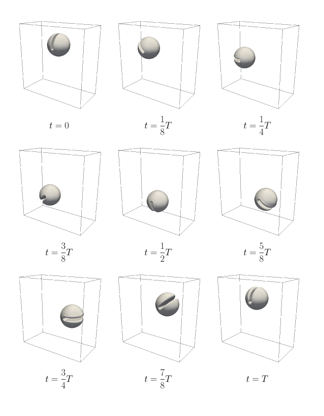
Figure 16: Evolution of test 2, calculated using the APPLIC method on a $200\times 200\times 96$ grid with $\Delta t=0.005$.

Figure 17 compares the initial (exact) shape and the final shapes using a $100\times 100\times 48$ ($\Delta x=0.01$) grid and $\Delta t=0.01$, where the maximum CFL number is approximately 0.5. The SVOF and VOF/WLIC methods produces significantly deformed shapes. Table 4 presents the $L_{1}$ errors and the corresponding convergence rates for $25\times 25\times 12$ $(\Delta x=0.04)$, $50\times 50\times 24$ $(\Delta x=0.02)$, and $100\times 100\times 48$ $(\Delta x=0.01)$, grids, where $\Delta t=0.04$, 0.02, and 0.01, respectively.

Figure 17: The initial $(t=0)$ and the final $(t=T)$ shapes for test 2, using a 100$\times$100$\times$48 grid with $\Delta t=0.01$.

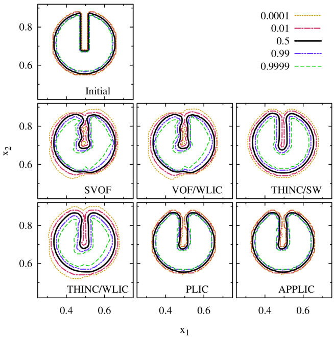
Figure 18:

Table 4: $L_{1}$ errors and convergence rates using different grid sizes for test 2.

Method	$25\times 25\times 12$	Rate	$50\times 50\times 24$	Rate	$100\times 100\times 48$
SVOF	$5.25\times 10^{-3}$	0.63	$3.40\times 10^{-3}$	1.32	$1.36\times 10^{-3}$
VOF/WLIC	$5.39\times 10^{-3}$	0.57	$3.63\times 10^{-3}$	1.35	$1.42\times 10^{-3}$
THINC/SW	$4.42\times 10^{-3}$	0.67	$2.79\times 10^{-3}$	1.50	$9.84\times 10^{-4}$
THINC/WLIC	$5.51\times 10^{-3}$	0.71	$3.36\times 10^{-3}$	1.30	$1.37\times 10^{-3}$
PLIC	$4.00\times 10^{-3}$	1.07	$1.91\times 10^{-3}$	1.58	$6.39\times 10^{-4}$
APPLIC	$3.99\times 10^{-3}$	0.98	$2.02\times 10^{-3}$	1.59	$6.73\times 10^{-4}$

3.1.3

In the third test problem, a sphere of 0.15 radius centered at $(0.35,0.35,0.35)$ in a computational domain $[0,1]\times[0,1]\times[0,1]$ is deformed in an incompressible flow field proposed by LeVeque [24], expressed by

$$u_{1} =2\sin^{2}(\pi x_{1})\sin(2\pi x_{2})\sin(2\pi x_{3})\cos(\pi t/T),$$ (52)

$$u_{2} =-\sin(2\pi x_{1})\sin^{2}(\pi x_{2})\sin(2\pi x_{3})\cos(\pi t/T),$$ (53)

$$u_{3} =-\sin(2\pi x_{1})\sin(2\pi x_{2})\sin^{2}(\pi x_{3})\cos(\pi t/T).$$ (54)

We set $T=3$. Figure 19 shows the evolution of the problem.

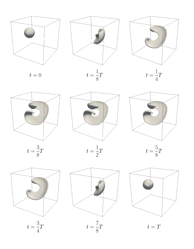
Figure 19: Evolution of test 3, calculated using the APPLIC method on a $200\times 200\times 200$ grid with $\Delta t=0.00125$.

Figure 20 compares the initial (exact) shape and the final shapes using a $100\times 100\times 100$ ($\Delta x=0.01$) grid with $\Delta t=0.0025$, where the maximum CFL number is approximately 0.5. The SVOF and the VOF/WLIC methods produces significantly deformed shapes. The shapes produced by the THINC/WLIC method have more prominent bumps than those by the PLIC and the APPLIC methods. Table 5 presents the $L_{1}$ errors and the corresponding convergence rates for $50\times 50\times 50$ $(\Delta x=0.02)$, $100\times 100\times 100$ $(\Delta x=0.01)$, and $200\times 200\times 200$ $(\Delta x=0.005)$ grids with $\Delta t=0.005$, 0.0025, and 0.00125, respectively.

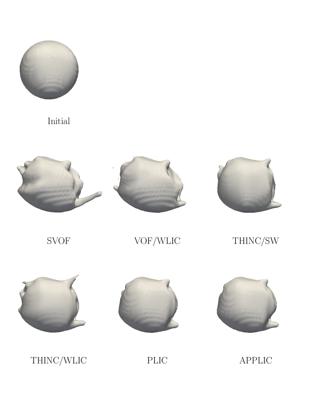
Figure 20: The initial $(t=0)$ and the final $(t=T)$ shapes for test 3, using a 100$\times$100$\times$100 grid with $\Delta t=0.0025$.

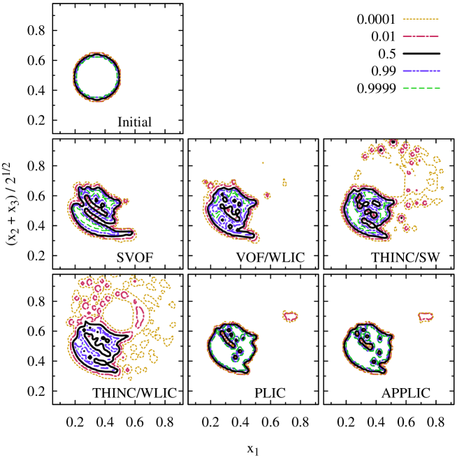
Figure 21:

Table 5: $L_{1}$ errors and convergence rates using different grid sizes for test 3.

Method	$25\times 25\times 25$	Rate	$50\times 50\times 50$	Rate	$100\times 100\times 100$
SVOF	$1.23\times 10^{-2}$	0.72	$7.47\times 10^{-3}$	1.21	$3.23\times 10^{-3}$
VOF/WLIC	$1.21\times 10^{-2}$	0.69	$7.49\times 10^{-3}$	1.30	$3.05\times 10^{-3}$
THINC/SW	$1.13\times 10^{-2}$	1.10	$5.24\times 10^{-3}$	1.69	$1.62\times 10^{-3}$
THINC/WLIC	$1.22\times 10^{-2}$	0.88	$6.62\times 10^{-3}$	1.64	$2.12\times 10^{-3}$
PLIC	$1.07\times 10^{-2}$	1.10	$4.98\times 10^{-3}$	2.04	$1.21\times 10^{-3}$
APPLIC	$1.05\times 10^{-2}$	1.04	$5.09\times 10^{-3}$	2.01	$1.26\times 10^{-3}$

3.2 Computational efficiency

We investigate the computational efficiency of the following method: VOF/WLIC, THIC/WLIC, PLIC, and APPLIC. The computational efficiency of the THINC/SW and the SVOF methods is comparable to that of the THINC/WLIC and the VOF/WLIC methods, respectively. The computational time required to evaluate fluxes for the 10,000,000 sample points in the set $S$, defined in section 2.3, for each method is used as a measure of efficiency.

The benchmark program is written in the C language. Calculations using both single-precision and double-precision floating point arithmetic were conducted. Three different computing platforms, summarized in Table 6, were used to measure computational times.

Table 6: Computing platforms to measure the computational time.

Platform	Computational processor	Compiler	Optimization options
I	Intel Xeon E5-2643 v3a	Intel C Compiler 16.0	-O3 -xCORE-AVX2
II	Vector processora of NEC SX-ACE	C++/SX 1.0	-pvctl,noverrchk
III	NVIDIA Tesla K40	nvcc in CUDA 7.5	-arch=sm_35
$\!\!\!{}^{\rm a}$Only one core was used.

The measured computational times are shown in Table 7 (single-precision) and in Table 8 (double-precision). As shown in the tables, the APPLIC method was 1.6-2.4 times faster than the PLIC method. The VOF/WLIC and the PLIC methods were the fastest and the slowest among the methods, respectively. Although the algorithm of the THINC/WLIC method is more simple than that of the APPLIC method, the computational times of the two methods were comparable. This is due to the calculations of transcendental functions, which are much more time-consuming than the basic arithmetic operations. To evaluate each flux, the THINC/WLIC and the APPLIC methods requires five (exp, log$\times 2$, and cosh$\times 2$) and four (exp$\times 2$ and log$\times 2$) transcendental functions, respectively.

Table 7: Computational times using single-precision floating point arithmetic.

	Computational times (ms)
Method	Platform I	Platform II	Platform III
VOF/WLIC	12.6	5.66	1.31
THINC/WLIC	78.4	57.5	1.74
PLIC	178.3	97.8	3.79
APPLIC	75.4	62.0	1.66

Table 8: Computational times using double-precision floating point arithmetic.

	Computational time (ms)
Method	Platform I	Platform II	Platform III
VOF/WLIC	25.7	7.07	2.67
THINC/WLIC	241.5	62.9	4.04
PLIC	440.3	117.0	7.55
APPLIC	195.6	75.2	4.15

4 Conclusions

We have presented a new PLIC-type VOF method called the APPLIC method. In this method, the complicated forward and inverse problems that arise with the PLIC method are approximately solved through the use of the extremely simple formulae. Accordingly, the APPLIC method is easier to develop and to maintain the computational codes than the standard PLIC method. The APPLIC method satisfies Eqs. (30)-(34), which are essential to be satisfied for any VOF methods.

We conducted computational tests to compare accuracy of the APPLIC method with other VOF methods; SVOF, VOF/WLIC, THINC/SW, THINC/WLIC, and PLIC. The results of the tests show that the APPLIC method is as accurate as the PLIC method and more accurate than the SVOF, VOF/WLIC, THINC/SW, and THINC/WLIC methods. It was demonstrated that the computational time of the APPLIC method is shorter than that of the PLIC method and comparable to that of the THINC/WLIC method.

Appendix A

In this appendix, we explain the derivation of Eq. (17) to evaluate $C_{\rm A}$.

The PLIC method assumes the shape of the dark fluid in the donor cell $\Omega$ as the intersection of $\Omega$ and an oriented plane $\{{\boldsymbol{x}}|\,{\boldsymbol{n}}\cdot{\boldsymbol{x}}<\alpha\}$. The SZ algorithms work with a unit cube and a normal vector ${\boldsymbol{m}}$ so that ${\boldsymbol{m}}\geq 0$ and $\|{\boldsymbol{m}}\|_{1}=1$. Therefore, we apply a coordinate transformation from ${\boldsymbol{x}}$ to ${\boldsymbol{x}}^{\prime}$ so that the donor cell $\Omega$ is mapped to the unit cube $\{{\boldsymbol{x}}^{\prime}\in[0,1]^{3}\}$, and the normal vector ${\boldsymbol{n}}$ is mapped to a vector ${\boldsymbol{m}}^{\prime}$ satisfying the relation ${\boldsymbol{m}}^{\prime}\geq 0$. The transformation, represented by $T_{0}$, is written as

$$x^{\prime}_{l} =\frac{\operatorname{sgn}n_{l}}{\Delta x}(x_{l}-\xi_{l}),$$ (55)

where ${\boldsymbol{\xi}}$ is the origin of the new coordinate, which is chosen from the eight vertices of $\Omega$ depending on the signs of $n_{1}$, $n_{2}$, and $n_{3}$ so that the image of the cell $\Omega$ coincides with the unit cube $\{{\boldsymbol{x}}^{\prime}\in[0,1]^{3}\}$. The vertex ${\boldsymbol{\xi}}$ is placed on the face $\phi^{*}$ if the signs of $m_{I}$ and $u_{I}$ are identical, or on the face $\phi$ otherwise. We can express the image of the oriented plane $\{{\boldsymbol{x}}|\,{\boldsymbol{n}}\cdot{\boldsymbol{x}}<\alpha\}$ under $T_{0}$ as $\{{\boldsymbol{x}}^{\prime}|\,{\boldsymbol{m}}^{\prime}\cdot{\boldsymbol{x}}^{\prime}<\alpha^{\prime}\}$, where $\alpha^{\prime}$ is the transformed plane constant. The vector ${\boldsymbol{m}^{\prime}}$ is given by

$$m^{\prime}_{l}=\dfrac{\dfrac{n_{l}\Delta x}{\operatorname{sgn}n_{l}}}{\Big{|}\dfrac{n_{1}\Delta x}{\operatorname{sgn}n_{1}}\Big{|}+\Big{|}\dfrac{n_{2}\Delta x}{\operatorname{sgn}n_{2}}\Big{|}+\Big{|}\dfrac{n_{3}\Delta x}{\operatorname{sgn}n_{3}}\Big{|}}=\frac{\lvert n_{l}\rvert}{\|{\boldsymbol{n}}\|_{1}}.$$ (56)

The plane constant $\alpha^{\prime}$ is determined by the solution of the inverse problem

$$\alpha^{\prime}=\alpha(C,{\boldsymbol{m}}^{\prime}).$$ (57)

Let $\Omega^{\prime}_{\rm A}$ be the image of $\Omega_{\rm A}$ under $T_{0}$. We apply a further coordinate transformation $T_{\rm A}$ from ${\boldsymbol{x}}^{\prime}$ to ${\boldsymbol{x}}^{\prime\prime}$ so that $\Omega^{\prime}_{\rm A}$ is mapped to the unit cube $\{{\boldsymbol{x}}^{\prime\prime}\in[0,1]^{3}\}$ and all the components of the transformed normal vector are nonnegative. The transformation $T_{\rm A}$ is written as

$$x^{\prime\prime}_{l}=\begin{cases}x^{\prime}_{l}&\text{if $l\neq I$},\\ {x^{\prime}_{l}}/{\lvert g\rvert}&\text{if $l=I$ and ${\boldsymbol{\xi}}$ is placed on $\phi$},\\ [{x^{\prime}_{l}-(1-\lvert g\rvert)}]/{\lvert g\rvert}&\text{if $l=I$ and ${\boldsymbol{\xi}}$ is placed on $\phi^{*}$}.\end{cases}$$ (58)

We can express the image of the oriented plane $\{{\boldsymbol{x}}^{\prime}|\,{\boldsymbol{m}}^{\prime}\cdot{\boldsymbol{x}}^{\prime}<\alpha^{\prime}\}$ under $T_{\rm A}$ as $\{{\boldsymbol{x}}^{\prime\prime}|\,{\boldsymbol{m}}^{\prime\prime}_{\rm A}\cdot{\boldsymbol{x}}^{\prime\prime}<\alpha^{\prime\prime}_{\rm A}\}$. The normal vector ${\boldsymbol{m}}^{\prime\prime}_{\rm A}$ and plane constant $\alpha^{\prime\prime}_{\rm A}$ are given by

$$m^{\prime\prime}_{{\rm A},l} =\begin{cases}Q^{\prime}_{\rm A}m^{\prime}_{l}\lvert g\rvert&\text{if $l=I$},\\ Q^{\prime}_{\rm A}m^{\prime}_{l}&\text{if $l\neq I$},\end{cases}$$ (59)

$$\alpha^{\prime\prime}_{\rm A} =\begin{cases}Q^{\prime}_{\rm A}[\alpha^{\prime}-m^{\prime}_{I}(1-\lvert g\rvert)]&\text{if $\xi$ is placed on $\phi^{*}$},\\ Q^{\prime}_{\rm A}\alpha^{\prime}&\text{if $\xi$ is placed on $\phi$},\end{cases}$$ (60)

where $Q^{\prime}_{\rm A}$ is the normalization factor determined by

$$Q^{\prime}_{\rm A} =\frac{1}{m^{\prime}_{1}+m^{\prime}_{2}+m^{\prime}_{3}-m^{\prime}_{I}+m^{\prime}_{I}\lvert g\rvert}$$

$$=\frac{1}{1-m^{\prime}_{I}(1-\lvert g\rvert)}.$$ (61)

Let $\Omega^{\prime\prime}_{\rm A}$ be the image of $\Omega^{\prime}_{\rm A}$ under $T_{\rm A}$. The volume of the shape $\Omega^{\prime\prime}_{\rm A}\cap\{{\boldsymbol{x}}^{\prime\prime}|\,{\boldsymbol{m}}^{\prime\prime}\cdot{\boldsymbol{x}}^{\prime\prime}<\alpha^{\prime\prime}\}$ in the ${\boldsymbol{x}}^{\prime\prime}$ coordinate system is determined by solving the forward problem $V(\alpha^{\prime\prime},{\boldsymbol{m}}^{\prime\prime})$. The partial volume fraction $C_{\rm A}$ is thus obtained via Eq. (17).

Appendix B

In this appendix, we derive the choice criterion $|\widetilde{\alpha}^{\prime\prime}_{\rm A}-1/2|>|\widetilde{\alpha}^{\prime\prime}_{\rm B}-1/2|$.

We define the approximation errors in $\widetilde{F}_{\rm A}$ and $\widetilde{F}_{\rm B}$ as

$$\varepsilon_{\rm A} =(\widetilde{F}_{\rm A}-F_{\rm PLIC})\operatorname{sgn}g,$$ (62)

$$\varepsilon_{\rm B} =(\widetilde{F}_{\rm B}-F_{\rm PLIC})\operatorname{sgn}g.$$ (63)

Because $F_{\rm PLIC}\operatorname{sgn}g=V(\alpha^{\prime\prime}_{\rm A},{\boldsymbol{m}}^{\prime\prime}_{\rm A})\lvert g\rvert=[C-(1-\lvert g\rvert)V(\alpha^{\prime\prime}_{\rm B},{\boldsymbol{m}}^{\prime\prime}_{\rm B})],$ we have

$$\varepsilon_{\rm A} =[\widetilde{V}(\widetilde{\alpha}^{\prime\prime}_{\rm A},{\boldsymbol{m}}^{\prime\prime}_{\rm A})-V(\alpha^{\prime\prime}_{\rm A},{\boldsymbol{m}}^{\prime\prime}_{\rm A})]\lvert g\rvert,$$ (64)

$$\varepsilon_{\rm B} =-[\widetilde{V}(\widetilde{\alpha}^{\prime\prime}_{\rm B},{\boldsymbol{m}}^{\prime\prime}_{\rm B})-V(\alpha^{\prime\prime}_{\rm B},{\boldsymbol{m}}^{\prime\prime}_{\rm B})](1-\lvert g\rvert),$$ (65)

where The aim of this appendix is to find a quick and easy criterion to guess whether $\lvert\varepsilon_{\rm A}\rvert<\lvert\varepsilon_{\rm B}\rvert$ or not.

The approximation error in $\widetilde{V}$ and $\widetilde{\alpha}$ are defined as

$$\varepsilon_{\alpha}(V,{\boldsymbol{m}}) =\widetilde{\alpha}(V,{\boldsymbol{m}})-\alpha(V,{\boldsymbol{m}}),$$ (66)

$$\varepsilon_{V}(\alpha,{\boldsymbol{m}}) =\widetilde{V}(\alpha,{\boldsymbol{m}})-V(\alpha,{\boldsymbol{m}}).$$ (67)

Using Eqs. (17b) and (17f), we obtain

$$\alpha^{\prime} =\widetilde{\alpha}^{\prime}-\varepsilon_{\alpha}(C,{\boldsymbol{m}}^{\prime}),$$ (68)

$$\alpha^{\prime\prime}_{\rm A} =\widetilde{\alpha}^{\prime\prime}_{\rm A}-Q^{\prime}_{\rm A}\varepsilon_{\alpha}(C,{\boldsymbol{m}}^{\prime}).$$ (69)

The approximation error $\varepsilon_{\rm A}$ is then given by

$$\varepsilon_{\rm A} =\{\widetilde{V}(\widetilde{\alpha}^{\prime\prime}_{\rm A},{\boldsymbol{m}}^{\prime\prime}_{\rm A})-V[\widetilde{\alpha}^{\prime\prime}_{\rm A}-Q^{\prime}_{\rm A}\varepsilon_{\alpha}(C,{\boldsymbol{m}}^{\prime}),{\boldsymbol{m}}^{\prime\prime}_{\rm A}]\}\lvert g\rvert$$

$$=\left[\varepsilon_{V}(\widetilde{\alpha}^{\prime\prime}_{\rm A},{\boldsymbol{m}}^{\prime\prime}_{\rm A})+Q^{\prime}_{\rm A}\varepsilon_{\alpha}(C,{\boldsymbol{m}}^{\prime})\frac{\partial}{\partial\alpha}{V}(\widetilde{\alpha}^{\prime\prime}_{\rm A},{\boldsymbol{m}}^{\prime\prime}_{\rm A})\right]\lvert g\rvert+O(Q^{\prime}_{\rm A}\lvert g\rvert\varepsilon_{\alpha}^{2}).$$ (70)

The value of $Q^{\prime}_{\rm A}\lvert g\rvert$ is included in the range $[0,1]$ because $m^{\prime}_{I}\in[0,1]$ and $\lvert g\rvert\in(0,1]$.

Let $V^{*}$ be an arbitrary value within $[0,1]$. The following relation holds:

$$\widetilde{V}[\widetilde{\alpha}(V^{*})]=V[{\alpha}(V^{*})]=V^{*},$$ (71)

Here the second arguments regarding ${\boldsymbol{m}}$ are omitted for brevity. On the other side, the following can be obtained:

$${V}[{\alpha}(V^{*})] ={V}[\widetilde{\alpha}^{*}-\varepsilon_{\alpha}(V^{*})]$$

$$={V}(\widetilde{\alpha}^{*})-\varepsilon_{\alpha}(V^{*})\frac{\partial}{\partial\alpha}{V}(\widetilde{\alpha}^{*})+O(\varepsilon_{\alpha}^{2}),$$ (72)

where $\widetilde{\alpha}^{*}$ stands for $\widetilde{\alpha}(V^{*})$. Using Eqs. (71) and (72), we have the relation between $\varepsilon_{V}$ and $\varepsilon_{\alpha}$ as

$$\varepsilon_{V}(\widetilde{\alpha}^{*})=-\varepsilon_{\alpha}(V^{*})\frac{\partial}{\partial\alpha}{V}(\widetilde{\alpha}^{*})+O(\varepsilon_{\alpha}^{2}).$$ (73)

Substituting Eq. (73) into (70) and neglecting the term $O(\varepsilon_{\alpha}^{2})$, we obtain

$$\varepsilon_{\rm A} \approx\lvert g\rvert\delta_{\rm A}\frac{\partial}{\partial\alpha}{V}(\widetilde{\alpha}^{\prime\prime}_{\rm A},{\boldsymbol{m}}^{\prime\prime}_{\rm A}),$$ (74)

with

$$\delta_{\rm A} =Q^{\prime}_{\rm A}\varepsilon_{\alpha}(C,{\boldsymbol{m}}^{\prime})-\varepsilon_{\alpha}(\widetilde{V}^{\prime\prime}_{\rm A},{\boldsymbol{m}}^{\prime\prime}_{\rm A}).$$ (75)

Similarly,

$$\varepsilon_{\rm B} \approx-(1-g)\delta_{\rm B}\frac{\partial}{\partial\alpha}{V}(\widetilde{\alpha}^{\prime\prime}_{\rm B},{\boldsymbol{m}}^{\prime\prime}_{\rm B}),$$ (76)

with

$$\delta_{\rm B} =Q^{\prime}_{\rm B}\varepsilon_{\alpha}(C,{\boldsymbol{m}}^{\prime})-\varepsilon_{\alpha}(\widetilde{V}^{\prime\prime}_{\rm B},{\boldsymbol{m}}^{\prime\prime}_{\rm B}).$$ (77)

Here $\widetilde{V}^{\prime\prime}_{\rm A}$ and $\widetilde{V}^{\prime\prime}_{\rm B}$ stand for $\widetilde{V}(\widetilde{\alpha}^{\prime\prime}_{\rm A},{\boldsymbol{m}}^{\prime\prime}_{\rm A})$ and $\widetilde{V}(\widetilde{\alpha}^{\prime\prime}_{\rm B},{\boldsymbol{m}}^{\prime\prime}_{\rm B})$, respectively.

The value of $\delta_{\rm A}$ becomes zero when $\lvert g\rvert$ is equal to one (because $\widetilde{V}^{\prime\prime}_{\rm A}=C$, ${\boldsymbol{m}}^{\prime\prime}_{\rm A}={\boldsymbol{m}}^{\prime}$, and $Q^{\prime}_{\rm A}=1$ if $\lvert g\rvert=1$). Similarly, $\delta_{\rm B}$ becomes zero when $\lvert g\rvert=0$. It is evident that $\delta_{\rm A}$ and $\delta_{\rm B}$ are smooth functions with respect to $\lvert g\rvert$. Considering these conditions, we adopt the following approximations:

$$\frac{\lvert\delta_{\rm A}\rvert}{\lvert\delta_{\rm A}\rvert+\lvert\delta_{\rm B}\rvert} \approx 1-\lvert g\rvert,$$ (78)

$$\frac{\lvert\delta_{\rm B}\rvert}{\lvert\delta_{\rm A}\rvert+\lvert\delta_{\rm B}\rvert} \approx\lvert g\rvert,$$ (79)

where we attach importance on simplicity rather than on accuracy. Figure 22 demonstrates the accuracy of the approximations. The data points are distributed roughly around the line $\lvert\delta_{\rm A}\rvert/({\lvert\delta_{\rm A}\rvert+\lvert\delta_{\rm B}\rvert})=1-\lvert g\rvert$.

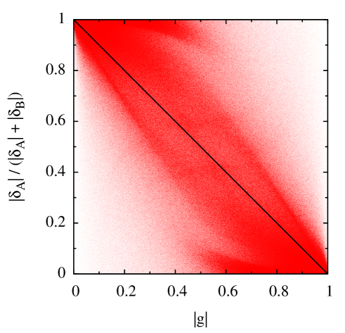
Figure 22: Plot of $\lvert g\rvert$ versus $\lvert\delta_{\rm A}\rvert/(\lvert\delta_{\rm A}\rvert+\lvert\delta_{\rm B}\rvert)$ for the sample points in the set $S$. In this plot, a small red dot is drawn for each point. The black solid line represents the line $\lvert\delta_{\rm A}\rvert/(\lvert\delta_{\rm A}\rvert+\lvert\delta_{\rm B}\rvert)=1-\lvert g\rvert$.

By use of Eqs. (78) and (79), the inequality $\lvert\varepsilon_{\rm A}\rvert<\lvert\varepsilon_{\rm B}\rvert$ can be written as

$$\frac{\partial}{\partial\alpha}{V}(\widetilde{\alpha}^{\prime\prime}_{\rm A},{\boldsymbol{m}}^{\prime\prime}_{\rm A})<\frac{\partial}{\partial\alpha}{V}(\widetilde{\alpha}^{\prime\prime}_{\rm B},{\boldsymbol{m}}^{\prime\prime}_{\rm B}),$$ (80)

We employ the following approximation for simplicity:

$$\frac{\partial}{\partial\alpha}{V}(\alpha,{\boldsymbol{m}}^{\prime\prime}_{\rm A})=\frac{\partial}{\partial\alpha}{V}(\alpha,{\boldsymbol{m}}^{\prime\prime}_{\rm B}),$$ (81)

where $\alpha$ is an arbitrary value. Because ${\partial V}/{\partial\alpha}$ is a monotonically nondecreasing function of $\alpha<1/2$ and has even symmetry to $\alpha=1/2$, inequality (80) becomes

$$\lvert\widetilde{\alpha}^{\prime\prime}_{\rm A}-1/2\rvert>\lvert\widetilde{\alpha}^{\prime\prime}_{\rm B}-1/2\rvert.$$ (82)

Thus we obtain the criterion.

References

- [1] C. W. Hirt, B. D. Nichols, Volume of fluid (VOF) method for the dynamics of free boundaries, Journal of Computational Physics 39 (1981) 201–225.
- [2] M. Rudman, Volume-tracking methods for interfacial flow calculations, International Journal for Numerical Methods in Fluids 24 (1997) 671–691.
- [3] W. J. Rider, D. B. Kothe, Reconstructing volume tracking, Journal of Computational Physics 141 (1998) 112–152.
- [4] R. Scardovelli, S. Zaleski, Direct numerical simulation of free-surface and interfacial flow, Annual Review of Fluid Mechanics 31 (1999) 567–603.
- [5] J. E. Pilliod Jr, E. G. Puckett, Second-order accurate volume-of-fluid algorithms for tracking material interfaces, Journal of Computational Physics 199 (2004) 465–502.
- [6] D. L. Youngs, Time-dependent multi-material flow with large fluid distortion, in: K. W. Morton, M. J. Baines (Eds.), Numerical Methods for Fluid Dynamics, Academic Press, New York, 1982, pp. 273–285.
- [7] J. Li, Calcul d’interface affine par morceaux (piecewise linear interface calculation), Comptes Rendus des Seances del’ Academie des Sciences Paris, Série IIb 320 (1995) 391–396.
- [8] W. F. Noh, P. Woodward, Slic (simple line interface method), Lecture Notes in Physics 24 (1976) 330–340.
- [9] K. Yokoi, Efficient implementation of THINC scheme: A simple and practical smoothed VOF algorithm, Journal of Computational Physics 226 (2007) 1985–2002.
- [10] M. Marek, W. Aniszewski, A. Bogusławski, Simplified volume of fluid method (SVOF) for two-phase flows, TASK Quarterly 12 (2008) 255–265.
- [11] F. Xiao, Y. Honma, T. Kono, A simple algebraic interface capturing scheme using hyperbolic tangent function, International Journal for Numerical Methods in Fluids 48 (2005) 1023–1040.
- [12] F. Xiao, S. Ii, C. Chen, Revisit to the THINC scheme: a simple algebraic vof algorithm, Journal of Computational Physics 230 (2011) 7086–7092.
- [13] S. Ii, K. Sugiyama, S. Takeuchi, S. Takagi, Y. Matsumoto, F. Xiao, An interface capturing method with a continuous function: The THINC method with multi-dimensional reconstruction, Journal of Computational Physics 231 (2012) 2328–2358.
- [14] R. Scardovelli, S. Zaleski, Analytical relations connecting linear interfaces and volume fractions in rectangular grids, Journal of Computational Physics 164 (2000) 228–237.
- [15] J. Hennessy, D. Patterson, Computer Architecture: A Quantitative Approach, The Morgan Kaufmann Series in Computer Architecture and Design, Elsevier Science, 2006.
- [16] R. Scardovelli, S. Zaleski, Interface reconstruction with least-square fit and split Eulerian–Lagrangian advection, International Journal for Numerical Methods in Fluids 41 (3) (2003) 251–274.
- [17] E. Aulisa, S. Manservisi, R. Scardovelli, S. Zaleski, Interface reconstruction with least-squares fit and split advection in three-dimensional Cartesian geometry, Journal of Computational Physics 225 (2) (2007) 2301–2319.
- [18] G. Weymouth, D. K.-P. Yue, Conservative Volume-of-Fluid method for free-surface simulations on Cartesian-grids, Journal of Computational Physics 229 (8) (2010) 2853–2865.
- [19] C. S. Wu, D. L. Young, H. C. Wu, Simulations of multidimensional interfacial flows by an improved volume-of-fluid method, International Journal of Heat and Mass Transfer 60 (2013) 739–755.
- [20] T. Vignesh, S. Bakshi, Noniterative interface reconstruction algorithms for volume of fluid method, International Journal for Numerical Methods in Fluids 73 (1) (2013) 1–18.
- [21] B. Parker, D. Youngs, Two and Three Dimensional Eulerian Simulation of Fluid Flow with Material Interfaces, Atomic Weapons Establishment, 1992.
- [22] D. Enright, R. Fedkiw, J. Ferziger, I. Mitchell, A hybrid particle level set method for improved interface capturing, Journal of Computational Physics 183 (1) (2002) 83–116.
- [23] S. T. Zalesak, Fully multidimensional flux-corrected transport algorithms for fluids, Journal of Computational Physics 31 (3) (1979) 335–362.
- [24] R. J. LeVeque, High-resolution conservative algorithms for advection in incompressible flow, SIAM Journal on Numerical Analysis 33 (2) (1996) 627–665.