Dark Radiation and Inflationary Freedom after Planck 2015

Abstract

The simplest inflationary models predict a primordial power spectrum (PPS) of the curvature fluctuations that can be described by a power-law function that is nearly scale-invariant. It has been shown, however, that the low-multipole spectrum of the CMB anisotropies may hint the presence of some features in the shape of the scalar PPS, which could deviate from its canonical power-law form. We study the possible degeneracies of this non-standard PPS with the active neutrino masses, the effective number of relativistic species and a sterile neutrino or a thermal axion mass. The limits on these additional parameters are less constraining in a model with a non-standard PPS when including only the temperature auto-correlation spectrum measurements in the data analyses. The inclusion of the polarization spectra noticeably helps in reducing the degeneracies, leading to results that typically show no deviation from the $\Lambda\textrm{CDM}$ model with a standard power-law PPS. These findings are robust against changes in the function describing the non-canonical PPS. Albeit current cosmological measurements seem to prefer the simple power-law PPS description, the statistical significance to rule out other possible parameterizations is still very poor. Future cosmological measurements are crucial to improve the present PPS uncertainties.

I Introduction

Inflation is one of the most successful theories that explains the so-called horizon and flatness problems, providing an origin for the primordial density perturbations that evolved to form the structures we observe today Guth (1981); Linde (1982); Starobinsky (1982); Hawking (1982); Albrecht and Steinhardt (1982); Mukhanov et al. (1992); Mukhanov and Chibisov (1981); Lucchin and Matarrese (1985); Lyth and Riotto (1999); Bassett et al. (2006); Baumann and Peiris (2009). The standard inflationary paradigm predicts a simple shape for the primordial power spectrum (PPS) of scalar perturbations: in this context, the PPS can be described by a power-law expression. However, there also exist more complicated inflationary scenarios which can give rise to non-standard PPS forms, with possible features at different scales, see e.g. Refs. Romano and Cadavid (2014); Kitazawa and Sagnotti (2014) and the reviews Martin et al. (2014); Chluba et al. (2015).

The usual procedure to reconstruct the underlying PPS is to assume a model for the evolution of the Universe and calculate the transfer function, and then use different techniques to constrain a completely unknown PPS, comparing the theoretical prediction with the measured power spectrum of the Cosmic Microwave Background radiation (CMB). Among the methods developed in the past, we can list regularization methods as the Richardson-Lucy iteration Shafieloo and Souradeep (2004); Nicholson and Contaldi (2009); Hazra et al. (2013, 2014), truncated singular value decomposition Nicholson et al. (2010) and Tikhonov regularization Hunt and Sarkar (2014, 2015), or methods as the maximum entropy deconvolution Goswami and Prasad (2013) or the cosmic inversion methods Matsumiya et al. (2002, 2003); Kogo et al. (2004, 2005); Nagata and Yokoyama (2008). Recently, the Planck collaboration presented a wide discussion about constraints on inflation Ade et al. (2015a). All these methods provide hint for a PPS which may not be as simple as a power-law. While the significance of the deviations is small for some cases, it is interesting to note that the CMB temperature power spectra as measured by both WMAP Bennett et al. (2013) and Planck Ade et al. (2014a); Adam et al. (2015) show similar results: the differences from the power-law are located in the low multipole region. These deviations could arise from some statistical fluctuations, or, instead, result from a non-standard inflationary mechanism.
If the features we observe are the result of a non-standard inflationary mechanism, we may be using an incomplete parameterization for the PPS in our cosmological analyses. It has been shown that this could lead to biased results in the cosmological constraints of different quantities. Namely, the constraints on the dark radiation properties de Putter et al. (2014); Gariazzo et al. (2015a); Di Valentino et al. (2015a) or on non-Gaussianities Gariazzo et al. (2015b) can be distorted, leading to spurious conclusions. In this work we aim to study the impact of a general PPS form in the constraints obtained for the properties of dark radiation candidates, such as the active neutrino masses and their effective number, sterile neutrino species and thermal axion properties. The outline of the Paper is as follows: we present the baseline standard $\Lambda\textrm{CDM}$  cosmological model, the PPS parameterization and the cosmological data in Sec. II. The results obtained within the $\Lambda\textrm{CDM}$ framework are presented in Sec. III. Concerning possible extensions of the $\Lambda\textrm{CDM}$ scenario, we study the constraints on the effective number of relativistic species in Sec. IV, on the neutrino masses in Sec. V, on massive neutrinos with a varying effective number of relativistic species in Sec. VI, on massive sterile neutrinos in Sec. VII, and on the thermal axion properties in Sec. VIII. Finally, in Sec. IX we show the reconstructed PPS shape, comparing different possible approaches, and we draw our conclusions in Sec. X.

II Baseline Model and Cosmological Data

In this Section we outline the baseline theoretical model that will be extended to study the dark radiation properties. For our analyses we use the numerical Boltzmann solver CAMB Lewis et al. (2000) for the theoretical spectra calculation, and the Markov Chain Monte Carlo (MCMC) algorithm CosmoMC Lewis and Bridle (2002) to sample the parameter space.

II.1 Standard Cosmological Model

The baseline model that we will extend to study various dark radiation properties is the $\Lambda\textrm{CDM}$ model, described by the six usual parameters: the current energy density of baryons and of Cold Dark Matter (CDM) ($\Omega_{b}h^{2}$, $\Omega_{c}h^{2}$), the ratio between the sound horizon and the angular diameter distance at decoupling ($\theta$), the optical depth to reionization ($\tau$), plus two parameters that describe the PPS of scalar perturbations, $P_{s}(k)$. The simplest models of inflation predict a power-law form for the PPS:

$$P_{s}(k)=A_{s}\left(k/k_{*}\right)^{n_{s}-1}\,,$$ (1)

where $k_{*}=0.05\,\text{Mpc}^{-1}$ is the pivot scale, while the amplitude ($A_{s}$) and the scalar spectral index ($n_{s}$) are free parameters in the $\Lambda\textrm{CDM}$ model. From these fundamental cosmological parameters we will compute other derived quantities, such as the Hubble parameter today $H_{0}$ and the clustering parameter $\sigma_{8}$, defined as the mean of matter fluctuations inside a sphere of 8$h$ Mpc radius.

From what concerns the remaining cosmological parameters, we follow the values of Ref. Ade et al. (2015b). In particular, unless they are freely varying, we consider the sum of the active neutrino masses to be $\Sigma m_{\nu}=0.06$ eV, and the effective number of relativistic species to be $N_{\rm{eff}}=3.046$ Mangano et al. (2005).

II.2 Primordial Power Spectrum of Scalar Perturbations

As stated before, possible hints of a non-standard PPS of scalar perturbations were found in several analyses, including both the WMAP and the Planck CMB spectra Shafieloo and Souradeep (2004); Nicholson and Contaldi (2009); Hazra et al. (2013, 2014); Nicholson et al. (2010); Hunt and Sarkar (2014, 2015); Goswami and Prasad (2013); Matsumiya et al. (2002, 2003); Kogo et al. (2004, 2005); Nagata and Yokoyama (2008); Ade et al. (2015a); Gariazzo et al. (2015a); Di Valentino et al. (2015a). From the theoretical point of view, there are plenty of well-motivated inflationary models that can give rise to non-standard PPS forms. Our major goal here is to study the robustness of the constraints on different cosmological quantities versus a change in the assumed PPS. Several cosmological parameters are known to present degeneracies with the standard PPS parameters, as, for example, the existing one between effective number of relativistic species $N_{\rm{eff}}$ and the tilt of the power-law PPS $n_{s}$. These degeneracies could be even stronger when more freedom is allowed for the PPS shape. We adopt here a non-parametric description for the PPS of scalar perturbations: we describe the function $P_{s}(k)$ as the interpolation among a series of nodes at fixed wavemodes $k$. Unless otherwise stated, we shall consider twelve nodes $k_{j}$ ($j\in[1,12]$) that cover a wide range of values of $k$: the most interesting range is explored between $k_{2}=0.001\,\text{Mpc}^{-1}$ and $k_{11}=0.35\,\text{Mpc}^{-1}$, that is approximately the range of wavemodes probed by CMB experiments. In this range we use equally spaced nodes in $\log k$. Additionally, we consider $k_{1}=5\times 10^{-6}\,\text{Mpc}^{-1}$ and $k_{12}=10\,\text{Mpc}^{-1}$ in order to ensure that all the PPS evaluations are inside the covered range. We expect that the nodes at these extreme wavemodes are unconstrained by the data.

Having fixed the position of all the nodes, the free parameters that are involved in our MCMC analyses are the values of the PPS at each node, $P_{s,j}=P_{s}(k_{j})/P_{0}$, where $P_{0}$ is the overall normalization, $P_{0}=2.2\times 10^{-9}$ Ade et al. (2015b). We use a flat prior in the interval $[0.01,10]$ for each $P_{s,j}$, for which the expected value will be close to 1.

The complete $P_{s}(k)$ is then described as the interpolation among the points $P_{s,j}$:

$$P_{s}(k)=P_{0}\times\texttt{PCHIP}(k;P_{s,1},\ldots,P_{s,12})\,,$$ (2)

where PCHIP is the piecewise cubic Hermite interpolating polynomial Fritsch and Carlson (1980); Fritsch and Butland (1984) (see also Ref. Gariazzo et al. (2015a) for a detailed description). In the following, when presenting our results, we will compare the constraints obtained in the context of the standard $\Lambda\textrm{CDM}$ model with a standard power-law PPS to those obtained with the free PCHIP PPS, described by (at least) sixteen free parameters ($\Omega_{b}h^{2}$, $\Omega_{c}h^{2}$, $\theta$, $\tau$, $P_{s,1},\ldots,P_{s,12}$). This minimal model will be extended to include the dark radiation properties we shall study in the various analyses.

The impact of the assumptions on the PPS parameterization will also be tested. We shall compare the results obtained with twelve nodes to the ones derived using a PCHIP PPS described by eight nodes. The position of these eight nodes $k_{j}^{(8)}$ is selected with the same rules as above: equally spaced nodes in $\log k$ between $k_{2}^{(8)}=k_{2}=0.001\,\text{Mpc}^{-1}$ and $k_{7}^{(8)}=k_{11}=0.35\,\text{Mpc}^{-1}$, plus the external nodes $k_{1}^{(8)}=k_{1}=5\times 10^{-6}\,\text{Mpc}^{-1}$ and $k_{8}^{(8)}=k_{12}=10\,\text{Mpc}^{-1}$.

To ease comparison bewteen the power-law and the PCHIP PPS approaches, we list in all the tables the results obtained for these two schemes. When considering a power-law PPS model, we show the constraints on $n_{s}$ and $A_{s}$, together with the values of the nodes $P_{s,1}^{\textrm{bf}}$ to $P_{s,12}^{\textrm{bf}}$ that would correspond to the best-fit values of $n_{s}$ and $A_{s}$ ($n_{s}^{\textrm{bf}}$ and $A_{s}^{\textrm{bf}}$). In other words, in each table presenting the marginalized constraints for the different cosmological parameters, in the columns corresponding to the analysis involving a power-law PPS, we shall list the values

$$P_{s,j}^{\textrm{bf}}\equiv\frac{A_{s}^{\textrm{bf}}}{P_{0}}\,\left(\frac{k_{j}}{k_{*}}\right)^{n_{s}^{\textrm{bf}}-1}\quad\mbox{ with }j\in[1,\ldots,12]\,,$$ (3)

that can be exploited for comparison purposes among the two PPS approaches.

II.3 Cosmological data

We base our analyses on the recent release from the Planck Collaboration Adam et al. (2015), that obtained the most precise CMB determinations in a very wide range of multipoles. We consider the full temperature power spectrum at multipoles $2\leq\ell\leq 2500$ (“Planck TT” hereafter) and the polarization power spectra in the range $2\leq\ell\leq 29$ (“lowP”). We shall also include the polarization data at $30\leq\ell\leq 2500$ (“TE, EE”) Aghanim et al. (2015). Since the polarization spectra at high multipoles are still under discussion and some residual systematics were detected by the Planck Collaboration Aghanim et al. (2015); Ade et al. (2015b), we shall use as baseline dataset the combination “Planck TT+lowP” . The impact of polarization measurements will be separately studied in the dataset “Planck TT,TE,EE+lowP”.

Additionally, we will consider the two CMB datasets above in combination with the following cosmological measurements:

• BAO: Baryon Acoustic Oscillations data as obtained by 6dFGS Beutler et al. (2011) at redshift $z=0.1$, by the SDSS Main Galaxy Sample (MGS) Ross et al. (2015) at redshift $z_{\rm{eff}}=0.15$ and by the BOSS experiment in the DR11 release, both from the LOWZ and CMASS samples Anderson et al. (2014) at redshift $z_{\rm{eff}}=0.32$ and $z_{\rm{eff}}=0.57$, respectively;

• MPkW: the matter power spectrum as measured by the WiggleZ Dark Energy Survey Parkinson et al. (2012), from measurements at four different redshifts ($z=0.22$, $z=0.41$, $z=0.60$ and $z=0.78$) for the scales $0.02\,h\,\mathrm{Mpc^{-1}}<k<0.2\,h\,\mathrm{Mpc^{-1}}$;

• lensing: the reconstruction of the lensing potential obtained by the Planck collaboration with the CMB trispectrum analysis Ade et al. (2015c).

III The $\Lambda\textrm{CDM}$ Model

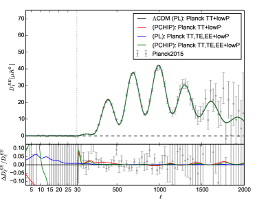
Figure 1: Comparison of the Planck 2015 data Adam et al. (2015) with the TT, TE and EE spectra obtained using the marginalized best-fit values from the analyses of Planck TT+lowP (black) and Planck TT,TE,EE+lowP (blue) in the $\Lambda\textrm{CDM}$ model with the power-law (PL) PPS, and from the analyses of Planck TT+lowP (red) and Planck TT,TE,EE+lowP (green) in the $\Lambda\textrm{CDM}$ model with the PCHIP PPS. The adopted values for each spectrum are reported in Tab. 1. We plot the $D_{\ell}=\ell(\ell+1)\,C_{\ell}/(2\pi)$ spectra and the relative (absolute for the case of the TE spectra) difference between each spectrum and the one obtained in the $\Lambda\textrm{CDM}$ (power-law PPS) model from the Planck TT+lowP data (black line).

In this section we shall consider a limited number of data combinations, including exclusively the datasets that can improve the constraints on the PCHIP PPS at small scales, namely, the Planck polarization measurements at high-$\ell$ and the MPkW constraints on the matter power spectrum.

The results we obtain for the $\Lambda\textrm{CDM}$ model are reported in Tab. 1 in the Appendix. In general, in the absence of high multipole polarization or large scale structure data, the parameter errors are increased. Those associated to $\Omega_{b}h^{2}$, $\Omega_{c}h^{2}$, $H_{0}$ and $\sigma_{8}$ show a larger difference, with deviations of the order of 1$\sigma$ in the PCHIP PPS case with respect to the power-law PPS case. The differences between the PCHIP and the power-law PPS parameterizations are much smaller for the “Planck TT,TE,EE+lowP+MPkW” dataset, and the two descriptions of the PPS give bounds for the $\Lambda\textrm{CDM}$ parameters tha fully agree. Therefore, the addition of the high multipole polarization spectra has a profound impact in our analyses, as we carefully explain in what follows. Figure 1 depicts the CMB spectra measured by Planck Adam et al. (2015), together with the theoretical spectra obtained from the best-fit values arising from our analyses. More concretely, we use the marginalized best-fit values reported in Tab. 1 for the $\Lambda\textrm{CDM}$ model with a power-law PPS obtained from the analyses of the Planck TT+lowP (in black) and Planck TT,TE,EE+lowP (in blue) datasets, plus the best-fit values in the $\Lambda\textrm{CDM}$ model with a PCHIP PPS, from the Planck TT+lowP (red) and Planck TT,TE,EE+lowP (green) datasets. We plot the $D_{\ell}=\ell(\ell+1)\,C_{\ell}/(2\pi)$ spectra of the TT, TE and EE anisotropies, as well as the relative (absolute for the TE spectra) difference between each spectrum and the one obtained from the Planck TT+lowP data in the $\Lambda\textrm{CDM}$ model with the power-law PPS. Notice that, in the case of the TT and EE spectra, the best-fit spectra are in good agreement with the observational data, even if there are variations among the $\Lambda\textrm{CDM}$ parameters, as they can be compensated by the freedom in the PPS. However, in the TE cross-correlation spectrum case, such a compensation is no longer possible: the inclusion of the TE spectrum in the analyses is therefore expected to have a strong impact on the derived bounds.

IV Effective Number of Relativistic Species

The amount of energy density of relativistic species in the Universe is usually defined as the sum of the photon contribution $\rho_{\gamma}$ plus the contribution of all the other relativistic species. This is described by the effective number of relativistic degrees of freedom $N_{\rm{eff}}$:

$$\rho_{\mathrm{rad}}=\left[1+\frac{7}{8}\left(\frac{4}{11}\right)^{4/3}N_{\rm{eff}}\right]\rho_{\gamma}\,,$$ (4)

where $N_{\rm{eff}}=3.046$ Mangano et al. (2005) for the three active neutrino standard scenario. Deviations of $N_{\rm{eff}}$ from its standard value may indicate that the thermal history of the active neutrinos is different from what we expect, or that additional relativistic particles are present in the Universe, as additional sterile neutrinos or thermal axions.

A non-standard value of $N_{\rm{eff}}$ may affect the Big Bang Nucleosynthesis era, and also the matter-radiation equality. A shift in the matter-radiation equality would cause a change in the expansion rate at decoupling, affecting the sound horizon and the angular scale of the peaks of the CMB spectrum, as well as in the contribution of the early Integrated Sachs Wolfe (ISW) effect to the CMB spectrum. To avoid such a shift and its consequences, it is possible to change simultaneously the energy densities of matter and dark energy, in order to keep fixed all the relevant scales in the Universe. In this case, the CMB spectrum will only be altered by an increased Silk damping at small scales (see e.g. Refs. Hou et al. (2013); Lesgourgues et al. (2013); Archidiacono et al. (2013a); Gariazzo et al. (2015c)).

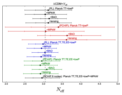
Figure 2: 68% and 95% CL constraints on $N_{\rm{eff}}$, obtained in the $\Lambda\textrm{CDM}$ + $N_{\rm{eff}}$ model. Different colors indicate Planck TT+lowP with PL PPS (black), Planck TT+lowP with PCHIP PPS (red), Planck TT,TE,EE+lowP with PL PPS (blue) and Planck TT,TE,EE+lowP with PCHIP PPS (green). For each color we plot 4 different datasets: from top to bottom, we have CMB only, CMB+MPkW, CMB+BAO and CMB+lensing. We also illustrate the results, in the context of the 8-nodes parameterization, for the Planck TT,TE,EE+lowP+MPkW dataset (last point in black).

The constraints on $N_{\rm{eff}}$ are summarized in Fig. 2, where we plot the 68% and 95% CL constraints on $N_{\rm{eff}}$ obtained with different datasets and PPS combinations for the $\Lambda\textrm{CDM}$ + $N_{\rm{eff}}$ model.

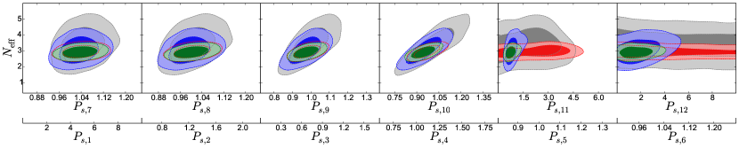
Figure 3: 68% and 95% CL constraints in the ($N_{\rm{eff}}$, $P_{s,j}$) planes, obtained in the $\Lambda\textrm{CDM}$ + $N_{\rm{eff}}$ model. We show the results for Planck TT+lowP (gray), Planck TT+lowP+MPkW (red), Planck TT,TE,EE+lowP (blue) and Planck TT,TE,EE+lowP+MPkW (green).

The introduction of $N_{\rm{eff}}$ as a free parameter does not change significantly the results for the $\Lambda\textrm{CDM}$ parameters if a power-law PPS is considered. However, once the freedom in the PPS is introduced, some degeneracies between the PCHIP  nodes $P_{s,j}$ and $N_{\rm{eff}}$ appear. Nevertheless, even if the constraints on $N_{\rm{eff}}$ are loosened for the PCHIP PPS case, all the dataset combinations give constraints on $N_{\rm{eff}}$ that are compatible with the standard value 3.046 at 95% CL, as we notice from Fig. 2 and Tab. 2 in the Appendix. The mild preference for $N_{\rm{eff}}>3.046$ arises mainly as a volume effect in the Bayesian analysis, since the PCHIP PPS parameters can be tuned to reproduce the observed CMB temperature spectrum for a wide range of values of $N_{\rm{eff}}$. As expected, the degeneracy between the nodes $P_{s,j}$ and $N_{\rm{eff}}$ shows up at high wavemodes, where the Silk damping effect is dominant, see Fig. 3. As a consequence of this correlation, the values preferred for the nodes $P_{s,6}$ to $P_{s,10}$ are slightly larger than the best-fit values in the power-law PPS at the same wavemodes. The cosmological limits for a number of parameters change as a consequence of the various degeneracies with $N_{\rm{eff}}$. For example, to compensate the shift of the matter-radiation equality redshift due to the increased radiation energy density, the CDM energy density $\Omega_{c}h^{2}$ mean value is slightly shifted and its constraints are weakened. At the same time, the uncertainty on the Hubble parameter $H_{0}$ is considerably relaxed, because $H_{0}$ must be also changed accordingly. The introduction of the polarization data helps in improving the constraints in the models with a PCHIP PPS, since the effects of increasing $N_{\rm{eff}}$ and changing the PPS are different for the temperature-temperature, the temperature-polarization and the polarization-polarization correlation spectra, as previously discussed in the context of the $\Lambda\textrm{CDM}$ model (see Tab. 3 in the Appendix): the preferred value of $N_{\rm{eff}}$ is very close to the standard value 3.046. Apparently, the Planck polarization data seem to prefer a value of $N_{\rm{eff}}$ slightly smaller than 3.046 for all the datasets except those including the BAO data, but the effect is not statistically significant (see the blue and green points in Fig. 2).

In conclusion, as the bounds for $N_{\rm{eff}}$ are compatible with 3.046, the $\Lambda\textrm{CDM}$ + $N_{\rm{eff}}$ model gives results that are very close to those obtained in the simple $\Lambda\textrm{CDM}$ model, but with slightly larger parameter uncertainties, in particular for $H_{0}$ and $\Omega_{c}h^{2}$.

V Massive Neutrinos

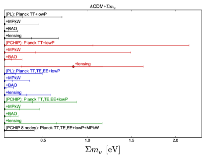
Figure 4: As Fig. 2 but for the $\Lambda\textrm{CDM}$ plus $\sum m_{\nu}$ case.

Neutrinos oscillations have robustly established the existence of neutrino masses. However, neutrino mixing data only provide information on the squared mass differences and not on the absolute scale of neutrino masses. Cosmology provides an independent tool to test it, as massive neutrinos leave a non negligible imprint in different cosmological observables Reid et al. (2010); Hamann et al. (2010); de Putter et al. (2012); Giusarma et al. (2013a); Zhao et al. (2013); Hou et al. (2014); Archidiacono et al. (2013b); Giusarma et al. (2013b); Riemer-Sørensen et al. (2014); Hu et al. (2014); Giusarma et al. (2014); Di Valentino et al. (2015b). The primary effect of neutrino masses in the CMB temperature spectrum is due to the early ISW effect. The neutrino transition from the relativistic to the non-relativistic regime affects the decay of the gravitational potentials at the decoupling period, producing an enhancement of the small-scale perturbations, especially near the first acoustic peak. A non-zero value of the neutrino mass also induces a higher expansion rate, which suppresses the lensing potential and the clustering on scales smaller than the horizon when neutrinos become non-relativistic. However, the largest effect of neutrino masses on the different cosmological observables comes from the suppression of galaxy clustering at small scales. After becoming non-relativistic, the neutrino hot dark matter relics possess large velocity dispersions, suppressing the growth of matter density fluctuations at small scales. The baseline scenario we analyze here has three active massive neutrino species with degenerate masses. In addition, we consider the PPS approach outlined in Sec. II. For the numerical analyses, when considering the power-law PPS, we use the following set of parameters:

$$\{\Omega_{b}h^{2},\Omega_{c}h^{2},\theta,\tau,n_{s},\log[10^{10}A_{s}],\Sigma m_{\nu}\}~{}.$$ (5)

We then replace the $n_{s}$ and $A_{s}$ parameters with the other twelve extra parameters ($P_{s,i}$ with $i=1,\ldots,12$) related to the PCHIP PPS parameterization. The 68% and 95% CL bounds on $\Sigma m_{\nu}$ obtained with different dataset and PPS combinations are summarized in Fig. 4.

Notice that, when considering Planck TT+lowP CMB measurements plus other external datasets, for all the data combinations, the bounds on neutrino masses are weaker when considering the PCHIP PPS with respect to the power-law PPS case (see also Tab. 4 in Appendix). Concerning CMB data only, the bound we find in the PCHIP approach is $\Sigma m_{\nu}<2.16$ eV at 95% CL, much less constraining than the bound $\Sigma m_{\nu}<0.75$ eV at 95% CL obtained in the power-law approach. This larger value is due to the degeneracy between $\Sigma m_{\nu}$ and the nodes $P_{s,5}$ and $P_{s,6}$, as illustrated in Fig. 5. In particular, these two nodes correspond to the wavenumbers where the contribution of the early ISW effect is located. Therefore, the change induced on these angular scales by a larger neutrino mass could be compensated by increasing $P_{s,5}$ and $P_{s,6}$. The addition of the matter power spectrum measurements, MPkW, leads to an upper bound on $\Sigma m_{\nu}$ of $1.15$ eV at 95% CL in the PCHIP parameterization, which is twice the value obtained when considering the power-law PPS with the same dataset. The most stringent constraints on the sum of the three active neutrino masses are obtained when we use the BAO data, since the geometrical information they provide helps breaking degeneracies among cosmological parameters. In particular, we have $\Sigma m_{\nu}<0.261$ eV ($\Sigma m_{\nu}<0.220$ eV) at 95% CL when considering the PCHIP (power-law) PPS parameterization. Finally, the combination of Planck TT+lowP data with the Planck CMB lensing measurements provide a bound on neutrino masses of $\Sigma m_{\nu}<1.64$ eV at 95% CL in the PCHIP case.

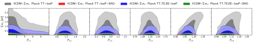
Figure 5: As Fig. 3 but for the $\Lambda\textrm{CDM}$ plus $\sum m_{\nu}$ case.

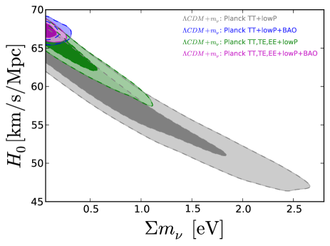
Figure 6: $68\%$ and $95\%$ CL allowed regions in the ($\Sigma m_{\nu}$, $H_{0}$) plane, using different combinations of datasets, within the PCHIP PPS parameterization.

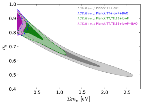
Figure 7: $68\%$ and $95\%$ CL allowed regions in the ($\Sigma m_{\nu}$, $\sigma_{8}$) plane, using different combinations of datasets, within the PCHIP PPS parameterization.

It can be noticed that in the PCHIP PPS there is a shift in the Hubble constant toward lower values. This occurs because there exists a strong, well-known degeneracy between the neutrino mass and the Hubble constant, see Fig. 6. In particular, considering CMB data only, a higher value of $\Sigma m_{\nu}$ will shift the location of the angular diameter distance to the last scattering surface, change that can be compensated with a smaller value of the Hubble constant $H_{0}$. The mean values of the clustering parameter $\sigma_{8}$ are also displaced by $\sim 2\sigma$ (except for the BAO case) toward lower values in the PCHIP PPS approach with respect to the mean values obtained when using the power-law PPS, as can be noticed from Fig. 7. Concerning the $P_{s,i}$ parameters, the bounds on $P_{s,i}$ with $i\geq 5$ are weaker with respect to the $\Lambda\textrm{CDM}$ case (see Tab. 1 in the Appendix), and only the combination of Planck TT+lowP data with the MPkW measurements provides an upper limit for the $P_{s,12}$ (concretely, $P_{s,12}<3.89$ at 95% CL).

Also when considering the high-$\ell$ polarization measurements, the bounds on the sum of the neutrino masses are larger when using the PCHIP parameterization with respect to the ones obtained with the power-law approach. However, these bounds are more stringent than those obtained using the Planck TT+lowP data only (see Tab. 5 in the Appendix). The reason for this improvement is due to the fact that the inclusion of the polarization measurements removes many of the degeneracies among the parameters. Concerning the CMB measurements only, we find an upper limit $\Sigma m_{\nu}<0.880$ eV at 95% CL in the PCHIP approach. The addition of the matter power spectrum measurements leads to a value of $\Sigma m_{\nu}<0.458$ eV at 95% CL in the PCHIP parameterization, improving the Planck TT,TE,EE+lowP constraint by a factor of two. Notice that, as in the Planck TT+lowP results, the data combination that gives the most stringent constraints is the one involving the Planck TT,TE,EE+lowP and BAO datasets, since it provides a 95% CL upper bound on $\Sigma m_{\nu}$ of 0.218 eV in the PCHIP PPS case. Finally, when the lensing measurements are added, the constraint on the neutrino masses is shifted to a higher value (agreeing with previous findings from the Planck collaboration), being $\Sigma m_{\nu}<1.17$ eV at 95% CL for the PCHIP case. The degeneracies between $\Sigma m_{\nu}$ and $H_{0}$, $\sigma_{8}$, even if milder than those without high multipole polarization data, are still present (see Figs. 6 and 7). The constraints on the $P_{s,i}$ parameters do not differ much from those obtained with the Planck TT+lowP data.

VI Effective Number of Relativistic Species and Neutrino Masses

After having analyzed the constraints on $N_{\rm{eff}}$ and $\Sigma m_{\nu}$ separately, we study in this section their joint constraints in the context of the $\Lambda\textrm{CDM}$ + $N_{\rm{eff}}$ + $\Sigma m_{\nu}$ extended cosmological model, focusing mainly on the differences with the results presented in the two previous sections.

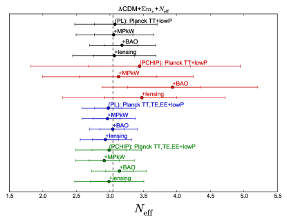
Figure 8: As Fig. 2 but for the $\Lambda\textrm{CDM}$ + $N_{\rm{eff}}$ + $\Sigma m_{\nu}$ model.

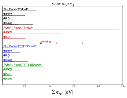
Figure 9: As Fig. 8, but for the $\Sigma m_{\nu}$ parameter.

The 68% and 95% CL constraints on $N_{\rm{eff}}$ and $\Sigma m_{\nu}$ are reported in Figs. 8 and 9 respectively, for different dataset combinations and PPS choices, see also Tabs. 6 and 7 in the Appendix. Notice that the qualitative conclusions drawn in the previous sections do not change here. The PCHIP PPS parameterization still allows for a significant freedom in the values of $N_{\rm{eff}}$ and $\Sigma m_{\nu}$, as these parameters have an impact on the CMB spectrum that can be easily mimicked by some variations in the PPS nodes. In particular, a significant degeneracy between $N_{\rm{eff}}$ and the nodes $P_{s,6}$ to $P_{s,10}$ appears, in analogy to what happens in the $\Lambda\textrm{CDM}$ + $N_{\rm{eff}}$ model (see Fig. 3 and the discussion in Sec. IV). At the same time, the strongest degeneracy involving the total neutrino mass appears between $\Sigma m_{\nu}$ and $P_{s,5}$. This corresponds to a rescaling of the PPS that compensates the change in the early ISW contribution driven by massive neutrinos (see Fig. 5 and the discussion in Sec. V). We do not show here the degeneracies with the $P_{s,i}$ nodes for the $\Lambda\textrm{CDM}$ + $N_{\rm{eff}}$ + $\Sigma m_{\nu}$ model, but we have verified that they are qualitatively similar to those depicted in Fig. 3 (Fig. 5) for the $N_{\rm{eff}}$ ($\Sigma m_{\nu}$) parameter. When considering CMB data only, the constraints are slightly loosened with respect to those obtained when the $N_{\rm{eff}}$ and $\Sigma m_{\nu}$ parameters are freely varied separately and not simultaneously. When comparing the power-law PPS and the PCHIP PPS models, we can notice that the variations of the neutrino parameters lead to several variations in other cosmological parameters. Such is the case of the baryon and CDM densities and the angular scale of the peaks, which are shifted by a significant amount, as a consequence of the degeneracies with both $N_{\rm{eff}}$ and $\Sigma m_{\nu}$. As the effects of $N_{\rm{eff}}$ and $\Sigma m_{\nu}$ on the Hubble parameter $H_{0}$ and the clustering parameter $\sigma_{8}$ are opposite, we find an increased uncertainty in these parameters, being their allowed ranges significantly enlarged.

While the tightest neutrino mass bound arises from the Planck TT+lowP+BAO dataset, the largest allowed mean value for $N_{\rm{eff}}$ is also obtained for this very same data combination ($N_{\rm{eff}}=3.94_{-0.67}^{+0.42}$ at 68% CL in the PCHIP PPS analysis), showing the large degeneracy between $\Sigma m_{\nu}$ and $N_{\rm{eff}}$. However, when including the Planck CMB lensing measurements, the trend is opposite to the one observed with the BAO dataset, with three times larger upper limits for $\Sigma m_{\nu}$ and lower mean values for $N_{\rm{eff}}$. As stated before, the fact that lensing data prefer heavier neutrinos is well known (see e.g. Sec. V and Refs. Ade et al. (2014b, 2015b)). Notice, from Fig. 9, that the only combination which shows a preference for $\Sigma m_{\nu}>0.06$ eV at 68% CL includes the lensing data ($\Sigma m_{\nu}=0.84^{+0.32}_{-0.62}$ eV, for the PCHIP PPS).

When polarization measurements are added in the data analyses, we obtain a 95% CL range of $2.5\lesssim N_{\rm{eff}}\lesssim 3.5$, with very small differences in both the central values and allowed ranges for the several data combinations explored here, see Tab. 7 in the Appendix. As in the $\Lambda\textrm{CDM}$ + $N_{\rm{eff}}$ model, the dataset including BAO data is the only one for which the mean value of $N_{\rm{eff}}$ is larger than 3, while in all the other cases it lies between 2.9 and 3. Apart from these small differences, all the results are perfectly in agreement with the standard value 3.046 within the 68% CL range. Concerning the $\Sigma m_{\nu}$ parameter, the results are also very similar to those obtained in the $\Lambda\textrm{CDM}$ + $\Sigma m_{\nu}$ model illustrated in Sec. V, with only very small differences in the exact numerical values of the derived bounds. The most constraining results are always obtained with the inclusion of BAO data, from which we obtain $\Sigma m_{\nu}<0.18\;(0.24)$ eV when using the power-law (PCHIP) PPS, both really close to the values derived in the $\Lambda\textrm{CDM}$ + $\Sigma m_{\nu}$ model.

For what concerns the remaining cosmological parameters, the differences between the power-law PPS and the PCHIP PPS results are much less significant when the polarization spectra are considered in the analyses. We may notice that the predicted values of the Hubble parameter $H_{0}$ are lower than the CMB estimates in the $\Lambda\textrm{CDM}$ model, and consequently they show an even stronger tension with local measurements of the Hubble constant. This is due to the negative correlation between $H_{0}$ and $\Sigma m_{\nu}$. On the other hand, the $\Lambda\textrm{CDM}$ + $N_{\rm{eff}}$ + $\Sigma m_{\nu}$ model predicts a $\sigma_{8}$ smaller than what is obtained in the $\Lambda\textrm{CDM}$ model for most of the data combinations, partially reconciling the CMB and the local estimates for this parameter.

The PCHIP nodes in this extended model do not deviate significantly from the expected values corresponding to the power-law PPS. The small deviations driven by the degeneracies with the neutrino parameters $\Sigma m_{\nu}$ and $N_{\rm{eff}}$ are canceled by the stringent bounds set by the polarization spectra, that break these degeneracies. Deviations from the power-law expectations are still visible at small wavemodes, corresponding to the dip at $\ell\simeq 20$ and to the small bump at $\ell\simeq 40$ in the CMB temperature spectrum.

VII Massive neutrinos and extra massive sterile neutrino species

Standard cosmology includes as hot thermal relics the three light, active neutrino flavors of the Standard Model of elementary particles. However, the existence of extra hot relic components, as dark radiation relics, sterile neutrino species and/or thermal axions is also possible. In their presence, the cosmological neutrino mass constraints will be changed. The existence of extra sub-eV massive sterile neutrino species is well motivated by the so-called short-baseline neutrino oscillation anomalies Abazajian et al. (2012); Kopp et al. (2013); Gonzalez-Garcia et al. (2015); Gariazzo et al. (2015c). These extra light species have an associated free streaming scale that will reduce the growth of matter fluctuations at small scales. They also contribute to the effective number of relativistic degree of freedom (i.e. to $N_{\rm{eff}}$).

We explore in this section the $\Lambda\textrm{CDM}$ scenario (in the two PPS parameterizations, power-law and PCHIP) with three active light massive neutrinos, plus one massive sterile neutrino species characterized by an effective mass $m_{s}^{\rm{eff}}$, that is defined by

$$m_{s}^{\rm{eff}}=\left(\frac{T_{s}}{T_{\nu}}\right)^{3}m_{s}=(\Delta N_{\rm{eff}})^{3/4}m_{s}~{},$$ (6)

where $T_{s}$ ($T_{\nu}$) is the current temperature of the sterile (active) neutrino species, $\Delta N_{\rm{eff}}\equiv N_{\rm{eff}}-3.046=(T_{s}/T_{\nu})^{3}$ is the effective number of degrees of freedom associated to the massive sterile neutrino, and $m_{s}$ is its physical mass. For the numerical analyses we use the following set of parameters to describe the model with a power-law PPS:

$$\{\Omega_{b}h^{2},\Omega_{c}h^{2},\theta,\tau,n_{s},\log[10^{10}A_{s}],\Sigma m_{\nu},N_{\rm{eff}},m_{s}^{\rm{eff}}\}~{}.$$ (7)

When considering the PCHIP PPS parameterization, $n_{s}$ and $A_{s}$ are replaced by the twelve parameters $P_{s,i}$ (with $i=1,\ldots,12$).

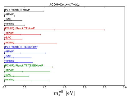
Figure 10: 68% and 95% CL constraints on $m_{s}^{\rm{eff}}$, obtained in the $\Lambda\textrm{CDM}$ + $N_{\rm{eff}}$ +$\Sigma m_{\nu}$+$m_{s}^{\rm{eff}}$model. Different colors indicate Planck TT+lowP with PL PPS (black), Planck TT+lowP with PCHIP PPS (red), Planck TT,TE,EE+lowP with PL PPS (blue) and Planck TT,TE,EE+lowP with PCHIP PPS (green). For each color we plot 4 different datasets: from top to bottom, we have CMB only, CMB+MPkW, CMB+BAO and CMB+lensing.

The 68% and 95% CL bounds on $m_{s}^{\rm{eff}}$ obtained with different datasets and PPS combinations are summarized in Fig. 10 and in Tabs. 8 and 9 in the Appendix. Notice that, in general, the value of $N_{\rm{eff}}$ is larger than in the case in which the sterile neutrinos are considered massless (see Tab. 2 in the Appendix). As for the other extensions of the $\Lambda\textrm{CDM}$ model we studied, the bounds on $\Sigma m_{\nu}$, $N_{\rm{eff}}$ and $m_{s}^{\rm{eff}}$ are weaker when considering the PCHIP PPS with respect to the ones obtained within the power-law PPS canonical scenario. Notice that the bounds on $m_{s}^{\rm{eff}}$ are not very stringent. This is due to the correlation between $m_{s}^{\rm{eff}}$ and $N_{\rm{eff}}$: sub-eV massive sterile neutrinos contribute to the matter energy density at recombination and therefore a larger value of $N_{\rm{eff}}$ will be required to leave unchanged both the angular location and the height of the first acoustic peak of the CMB.

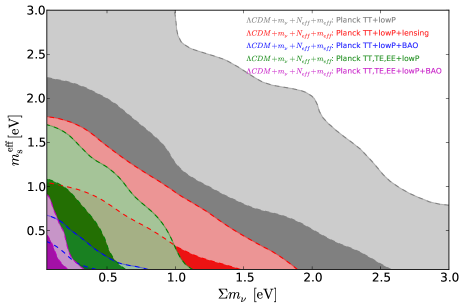
Figure 11: $68\%$ and $95\%$ CL allowed regions in the ($\Sigma m_{\nu}$, $m_{s}^{\rm{eff}}$) plane using the different combination of datasets, within the PCHIP PPS parameterization.

Figure 11 illustrates the degeneracy between the active and the sterile neutrino masses. Since both active and sterile sub-eV massive neutrinos contribute to the matter energy density at decoupling, an increase of $m_{s}^{\rm{eff}}$ can be compensated by lowering $\Sigma m_{\nu}$, in order to keep fixed the matter content of the universe. Notice that the most stringent $95\%$ CL bounds on the three active and sterile neutrinos are obtained considering the BAO data in the two PPS cases. In particular, we find $\Sigma m_{\nu}<0.481$ eV, $m_{s}^{\rm{eff}}<0.448$ eV for the PCHIP parametrization and $\Sigma m_{\nu}<0.263$ eV, $m_{s}^{\rm{eff}}<0.449$ eV for the power-law approach. Furthermore, in general, when considering the PCHIP parametrization, the mean value on the Hubble constant is smaller than the value obtained in the standard power-law PPS framework, due to the strong degeneracy between $\Sigma m_{\nu}$ and $H_{0}$. The value of the clustering parameter $\sigma_{8}$ is reduced in the two PPS parameterizations when comparing to the massless sterile neutrino case. This occurs because the sterile neutrino mass is another source of suppression of the large scale structure growth.

The inclusion of the polarization data improves notably the constraints on the cosmological parameters in the model with a PCHIP parametrization. In particular, the neutrino constraints are stronger than those obtained using only the temperature power spectrum at small angular scales. This effect is related to the fact that many degeneracies are reduced by the high multipole polarization measurements (as, for example, the one between $\Sigma m_{\nu}$ and $\tau$). Concerning the CMB measurements only, we find an upper limit on the three active and sterile neutrino masses of $\Sigma m_{\nu}<0.83$ eV and $m_{s}^{\rm{eff}}<1.20$ eV at 95% CL, while for the effective number of relativistic degrees of freedom we obtain $N_{\rm{eff}}<3.67$ at 95% CL, considering the PCHIP PPS approach. Also in this case the most stringent constraints are obtained when adding the BAO datasets to the Planck TT,TE,EE+lowP data. Finally, the addition of the lensing potential displaces both the active and sterile neutrino mass constraints to higher values.

Concerning the $P_{s,i}$ parameters, we can notice that considering the Planck TT,TE,EE+lowP+BAO datasets, the dip corresponding to the $P_{s,3}$ node is reduced with respect to the other possible data combinations. We have an upper bound for the $P_{s,12}$ node from all the data combinations except for the CMB+lensing dataset combination. In addition, as illustrated in Secs. V and VI, a significant degeneracy between $N_{\rm{eff}}$ and the nodes $P_{s,8}$ to $P_{s,10}$ and between $\Sigma m_{\nu}$ and the nodes $P_{s,5}$ and $P_{s,6}$ is also present in this $\Lambda\textrm{CDM}$ extension. Finally, because of the correlation between $\Sigma m_{\nu}$ and $m_{s}^{\rm{eff}}$, degeneracies between $m_{s}^{\rm{eff}}$ and the nodes $P_{s,5}$ and $P_{s,6}$ will naturally appear.

VIII Thermal Axion

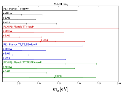
Figure 12: As Fig. 2 but in the context of the $\Lambda\textrm{CDM}$ + $m_{a}$ model, focusing on the thermal axion mass $m_{a}$ parameter.

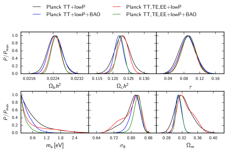
Figure 13: One-dimensional posterior probability for some cosmological parameters for the combination of datasets labeled in the figure, for the power-law approach in the $\Lambda\textrm{CDM}$ + $m_{a}$ scenario.

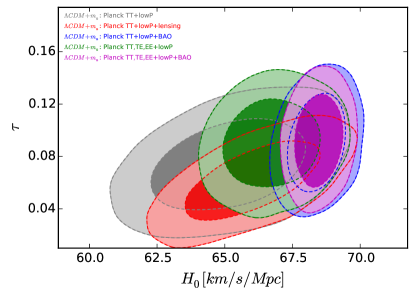
Figure 14: $68\%$ and $95\%$ CL allowed regions in the ($H_{0}$, $\tau$) plane using the different combinations of datasets in the $\Lambda\textrm{CDM}$ + $m_{a}$ model with a PCHIP PPS.

The axion field arises from the solution proposed by Peccei and Quinn Peccei and Quinn (1977a, b); Weinberg (1978); Wilczek (1978) to solve the strong CP problem in Quantum Chromodynamics. They introduced a new global Peccei-Quinn symmetry $U(1)_{PQ}$ that, when spontaneously broken at an energy scale $f_{a}$, generates a Pseudo-Nambu-Goldstone boson, the axion particle. Depending on the production process in the early universe, thermal or non-thermal, the axion is a possible candidate for an extra hot thermal relic, together with the relic neutrino background, or for the cold dark matter component, respectively. In what follows, we shall focus on the thermal axion scenario. The axion coupling constant $f_{a}$ is related to the thermal axion mass via

$$m_{a}=\frac{f_{\pi}m_{\pi}}{f_{a}}\frac{\sqrt{R}}{1+R}=0.6\ {\rm eV}\ \frac{10^{7}\,{\rm GeV}}{f_{a}}~{},$$ (8)

with $R=0.553\pm 0.043$, the up-to-down quark masses ratio, and $f_{\pi}=93$ MeV, the pion decay constant. Considering other values of $R$ within the range $0.38-0.58$ Olive et al. (2014) does not affect in a significant way this relationship (Archidiacono et al., 2015).

When the thermal axion is still a relativistic particle, it increases the effective number of relativistic degrees of freedom $N_{\rm{eff}}$, enhancing the amount of radiation in the early universe, see Eq. (4). It is possible to compute the contribution of a thermal axion as an extra radiation component as:

$$\Delta N_{\rm{eff}}=\frac{4}{7}\left(\frac{3}{2}\frac{n_{a}}{n_{\nu}}\right)^{4/3}~{},$$ (9)

with $n_{a}$ the current axion number density and $n_{\nu}$ the present neutrino plus antineutrino number density per flavor. When the thermal axion becomes a non relativistic particle, it increases the amount of the hot dark matter density in the universe, contributing to the total mass-energy density of the universe. Thermal axions promote clustering only at large scales, suppressing the structure formation at scales smaller than their free-streaming scale, once the axion is a non-relativistic particle. Several papers in the literature provide bounds on the thermal axion mass, see for example Refs. Melchiorri et al. (2007); Hannestad et al. (2007, 2008, 2010); Archidiacono et al. (2013c); Giusarma et al. (2014); Di Valentino et al. (2015c). In this paper our purpose is to update the work done in Ref. Di Valentino et al. (2015a), in light of the recent Planck 2015 temperature and polarization data Adam et al. (2015). Therefore, in what follows, we present up-to-date constraints on the thermal axion mass, relaxing the assumption of a power-law for the PPS of the scalar perturbations, assuming also the PCHIP PPS scenario.

The bounds on the axion mass are relaxed in the PCHIP PPS scenario, as illustrated in Fig. 12 (see also Tabs. 10 and 11 in the Appendix). This effect is related to the relaxed bound we have on $N_{\textrm{eff}}$ when letting it free to vary in an extended $\Lambda\textrm{CDM}$ + $N_{\textrm{eff}}$ scenario. From the results presented in Tab. 2, we find $N_{\textrm{eff}}=3.40_{-1.43}^{+1.50}$ at $95\%$ CL for the PCHIP PPS parameterization, implying that the PCHIP formalism favours extra dark radiation, and therefore a higher axion mass will be allowed. As a consequence, we find that the axion mass is totally unconstrained using the Planck TT+lowP data in the PCHIP PPS approach. We instead find the bound $m_{a}<1.97$ eV at $95\%$ CL for the standard power-law case. The most stringent bounds arise when using the BAO data, since they are directly sensitive to the free-streaming nature of the thermal axion. While the MPkW measurements are also sensitive to this small scale structure suppression, BAO measurements are able to constrain better the cold dark matter density $\Omega_{c}h^{2}$, strongly correlated with $m_{a}$. We find $m_{a}<0.93$ eV at $95\%$ CL in the standard case, and a slightly weaker constraint in the PCHIP case, $m_{a}<1.07$ eV at $95\%$ CL. Finally, when considering the lensing dataset, we obtain $m_{a}<1.45$ eV at $95\%$ CL in the power-law PPS case, bound that is relaxed in the PCHIP PPS, $m_{a}<2.15$ eV at $95\%$ CL. For this combination of datasets, a mild preference appears for an axion mass different from zero ($m_{a}=1.05_{-0.81}^{+0.37}$ at $68\%$ CL), only when considering the PCHIP approach, as illustrated in Fig. 12. This is probably due to the existing tension between the Planck lensing reconstruction data and the lensing effect, see Refs. Ade et al. (2015b); Di Valentino et al. (2015d).

The weakening of the axion mass constraints in most of the data combinations obtained in the PCHIP PPS scheme is responsible for the shift at more than 1$\sigma$ in the cold dark matter mass-energy density, due to the existing degeneracy between $m_{a}$ and $\Omega_{c}h^{2}$. Interestingly, this effect has also an impact on the Hubble constant, shifting its mean value by about 2$\sigma$ towards lower values, similarly to the results obtained in the neutrino mass case. Furthermore, a shift in the optical depth towards a lower mean value is also present when analyzing the PCHIP PPS scenario. One can explain this shift via the existing degeneracies between $\tau$ and $H_{0}$ and between $\tau$ and $\Omega_{c}h^{2}$. Once BAO measurements are included in the data analyses, the degeneracies are however largely removed and there is no significant shift in the values of the $\Omega_{c}h^{2}$, $H_{0}$ and $\tau$ parameters within the PCHIP PPS approach, when compared to their mean values in the power-law PPS. Concerning the $P_{s,i}$ parameters, we can observe also in this $\Lambda\textrm{CDM}$ + $m_{a}$ scenario a dip (corresponding to the $P_{s,3}$ node) and a bump (corresponding to the $P_{s,4}$ node), see Tabs. 10 and 11 in the Appendix. These features are more significant for the case of CMB data only.

In general, the constraints arising from the addition of high-$\ell$ polarization measurements are slightly weaker than those previously obtained. The weakening of the axion mass is driven by the preference of Planck TT,TE,EE+lowP for a lower value of $N_{\textrm{eff}}$, as pointed out before. As shown in Ref. Di Valentino et al. (2015a), the additional contribution to $N_{\textrm{eff}}$ due to thermal axions is a steep function of the axion mass, at least for low thermal axion masses (i.e. below $\sim 1$eV). The lower value of $N_{\textrm{eff}}$ preferred by small-scale polarization dramatically sharpens the posterior of $m_{a}$ at low mass (see Fig. 13). At higher masses, axions contribute mostly as cold dark matter: the posterior distribution flattens and overlaps with the one resulting from Planck TT+lowP, since CMB polarization does not help in improving the constraints on $\Omega_{m}$ (notice the presence of a bump in the posterior distributions of $\Omega_{m}$ and $\sigma_{8}$ for Planck TT,TE,EE+lowP). The mismatch in the values of $\Omega_{m}$ preferred by low and high thermal axion masses leads to a worsening in the constraints on $m_{a}$ with respect to the Planck TT+lowP scenario, since the volume of the posterior distribution is now mainly distributed at higher masses. When BAO data are considered, we get the tightest bounds on $m_{a}$. This is due to the fact that BAO measurements allow to constrain better $\Omega_{m}$, excluding the high mass axion region. In addition, the bump in both the $\Omega_{m}$ and $\sigma_{8}$ distributions disappears completely, due to the higher constraining power on the clustering parameter and the matter density. As can be noticed from Fig. 13, the tail of the $m_{a}$ distribution is excluded when adding BAO measurements.

Furthermore, the thermal axion mass bounds are relaxed within the PCHIP PPS formalism. In particular, concerning the CMB measurements only, $m_{a}<2.44$ eV at $95\%$ CL in the PCHIP approach, compared to the bound $m_{a}<2.09$ eV at $95\%$ CL in the standard power-law PPS description. When adding the matter power spectrum measurements (MPkW) we find upper limits on the axion mass that are $m_{a}<1.19$ eV at $95\%$ CL in the power-law PPS and $m_{a}<1.90$ eV at $95\%$ CL in the PCHIP parametrization. When considering the lensing dataset, we obtain $m_{a}<1.68$ eV at $95\%$ CL in the power-law PPS case, that is relaxed in the PCHIP PPS, $m_{a}<2.44$ eV at $95\%$ CL. A mild preference for an axion mass different from zero appears from this particular data combination ($m_{a}=1.39_{-0.63}^{+0.71}$ at $68\%$ CL) only when considering a PCHIP approach, see Fig. 12.

It is important to note that, when high multipole polarization data is included, there is no shift induced neither in the mean value of the optical depth nor in the one corresponding to the cold dark matter energy density in the PCHIP approach (with respect to the power-law case). High $\ell$ polarization data is extremely powerful in breaking degeneracies, as, for instance, the one existing between $\tau$ and $H_{0}$, as noticed from Fig. 14.

Interestingly, varying the thermal axion mass has a significant effect in the $\sigma_{8}-\Omega_{m}$ plane in both PPS approaches, see Fig. 15, weakening the bounds found for the $\Lambda\textrm{CDM}$ model and pushing the $\sigma_{8}$ ($\Omega_{m}$) parameter towards a lower (higher) value. Concerning the $P_{s,i}$ parameters, the bounds on the nodes remain unchanged after adding the high-$\ell$ polarization data (when they are compared to the Planck TT+lowP baseline case). The significance of the dip and the bump are also very similar for the different datasets.

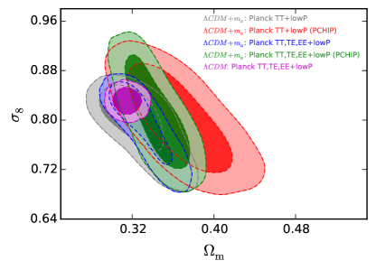
Figure 15: $68\%$ and $95\%$ CL allowed regions in the ($\Omega_{m}$, $\sigma_{8}$) plane using the different combinations of datasets in the $\Lambda\textrm{CDM}$ + $m_{a}$ model.

We have also explored the case in which both massive neutrinos and a thermal axion contribute as possible hot dark matter candidates. Our results, not illustrated here, show that the thermal axion mass bounds are unchanged in the extended $\Lambda\textrm{CDM}$ + $m_{a}$ + $\Sigma m_{\nu}$ model with respect to the $\Lambda\textrm{CDM}$ + $m_{a}$ scenario, leading to almost identical axion mass contraints. On the other hand, the presence of thermal axions tightens the neutrino mass bounds, as these two thermal relics behave as hot dark matter with a free-streaming nature. The most stringent bounds on both the axion mass and on the total neutrino mass arise, as usual, from the addition of BAO data. We find $m_{a}<1.18$ eV at $95\%$ CL and $\Sigma m_{\nu}<0.180$ eV at $95\%$ CL in the PCHIP PPS when combining BAO with the Planck TT,TE,EE+lowP datasets.

IX Primordial Power Spectrum Results

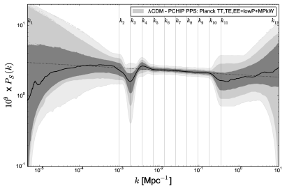
Figure 16: Reconstruction of the marginalized best fit PCHIP PPS (solid line) with 68%, 95% and 99% confidence bands as obtained in the $\Lambda\textrm{CDM}$ model, with the “’Planck TT,TE,EE+lowP+MPkW” dataset. The dotted line represents the power-law PPS corresponding to the Planck best fit Ade et al. (2015b).

From the MCMC analyses presented in the previous sections we obtained constraints on the nodes used to parameterize the PCHIP PPS. Using these information, we can obtain a reconstruction of the spectrum shape for the different extensions of the $\Lambda\textrm{CDM}$ model. Since the form of the reconstructed PPS is similar for the different models, we discuss now the common features of the PCHIP PPS as obtained for the $\Lambda\textrm{CDM}$ model. We shall comment on the results for the dataset combinations shown in Tab. 1: Planck TT+lowP, Planck TT,TE,EE+lowP, Planck TT+lowP+MPkW and Planck TT,TE,EE+lowP+MPkW. Figure 16 illustrates the results for this last dataset combination. For all datasets the nodes $P_{s,1}$ and $P_{s,12}$ are badly constrained, due to the fact that these nodes are selected to cover a wide range of wavemodes for computational reasons, but there are no available data to constrain them directly. Also the node $P_{s,11}$ is not very well constrained by the Planck temperature data, however the bounds on $P_{s,11}$ and $P_{s,12}$ can be improved with the inclusion of the high-multipole polarization data (TE,EE), leading to a significant improvement for $P_{s,11}$. The inclusion of the MPkW data allows to further tighten the constraints on the last two nodes of the PCHIP PPS parameterization, see Fig. 16. The impact of the polarization on the nodes located at high $k$ is smaller than the one due to the addition of the matter power spectrum data, since the MPkW dataset provides very strong constraints on the smallest angular scales.

The bounds on the nodes at small wavemodes ($P_{s,1}$ to $P_{s,4}$) are almost insensitive to the inclusion of additional datasets or to the change in the underlying cosmological model, with only small variations inside the 1$\sigma$ range between the different results. The error bars on the nodes are larger in this part of the spectrum, since it corresponds to low multipoles in the CMB power spectra, where cosmic variance is larger. In this part of the PPS we have the most evident deviations from the simple power-law PPS. The features are described by the node $P_{s,3}$, for which the value corresponding to the power-law PPS is approximately $2\sigma$ away from the reconstructed result, and by the node $P_{s,4}$, which is mildly discrepant with the power-law value ($1\sigma$ level). These nodes describe the behavior of the CMB temperature spectrum at low-$\ell$, where the observations of the Planck and WMAP experiments show a lack of power at $\ell\simeq 20$ and an excess of power at $\ell\simeq 40$. The detection of these features is in agreement with several previous studies Shafieloo and Souradeep (2004); Nicholson and Contaldi (2009); Hazra et al. (2013, 2014); Nicholson et al. (2010); Hunt and Sarkar (2014, 2015); Goswami and Prasad (2013); Matsumiya et al. (2002, 2003); Kogo et al. (2004, 2005); Nagata and Yokoyama (2008); Ade et al. (2015a); Gariazzo et al. (2015a); Di Valentino et al. (2015a) .

The central part of the reconstructed PPS, from $P_{s,5}$ to $P_{s,10}$, is very well constrained by the data. In this range of wavemodes, no deviations from the power-law PPS are visible, thus confirming the validity of the assumption that the PPS is almost scale-invariant for a wide range of wavemodes. This is also the region where the PPS shape is more sensitive to the changes in the $\Lambda\textrm{CDM}$ model caused by its extensions.

As we can see from the results presented in previous sections, the constraints on the nodes $P_{s,5}$ to $P_{s,10}$ are different for each extension of the $\Lambda\textrm{CDM}$ model, in agreement with the results obtained for $\ln[10^{10}A_{s}]$ and $n_{s}$ when considering the power-law PPS. The value of the power-law PPS normalized to match the values of the PCHIP nodes can be calculated by means of the relation $P_{s}(k)=A_{s}(k/k_{*})^{n_{s}-1}/P_{0}$: at each scale $k$, the value $P_{s}(k)$ is influenced both from $A_{s}$ and $n_{s}$, since $P_{0}$ and $k_{*}$ are fixed. In the various tables, when presenting the results on the power-law PPS, we listed the values of the PCHIP nodes that would correspond to the best-fitting $A_{s}$ and $n_{s}$, to help in the comparison with the PCHIP PPS constraints. These values are calculated using Eq. (3). In the range between $k\simeq 0.007$ and $k\simeq 0.2$, the constraints in the PCHIP nodes correspond, for most of the cases, to the values expected by the power-law PPS analyses, within their allowed 1$\sigma$ range. There are a few exceptions: for example, in the $\Lambda\textrm{CDM}$ + $N_{\rm{eff}}$ model and with the Planck TT+lowP+BAO dataset, the node $P_{s,10}$ deviates from the expected value corresponding to the power-law PPS by more than 1$\sigma$ (see Tab. 2). This is a consequence of the large correlation and the large variability range that this dataset allows for $N_{\rm{eff}}$. A similar behavior appears in the $\Lambda\textrm{CDM}$ + $N_{\rm{eff}}$+ $\Sigma m_{\nu}$ model (see Tab. 6) and in the $\Lambda\textrm{CDM}$ + $\Sigma m_{\nu}$+ $N_{\rm{eff}}$+ $m_{s}^{\rm{eff}}$ model (Tab. 8), for the same reasons. The inclusion of polarization data at high-$\ell$, limiting the range for $N_{\rm{eff}}$, does not allow for these deviations from the power-law PPS.

It is interesting to study how the previous findings depend on the choice of the PPS parameterization. One could ask then how many nodes are needed to capture hints for unexplored effects, which could be due to unaccounted systematics, or, more interestingly, to new physics. A number of nodes larger than the one explored here (12 nodes) becomes unfeasible, as it would be extremely challenging computationally. However, lowering the number of nodes would be a very efficient solution for practical purposes, assuming the hints previously found are not totally diluted. We have therefore checked this alternative scenario, using eight nodes, as described in Sec. II.2. The constraints on the PPS derived using this parameterization are reported in Fig. 17, obtained considering the $\Lambda\textrm{CDM}$ model and the Planck TT,TE,EE+lowP+MPkW dataset. The PCHIP parameterization with only eight nodes is not able to catch the features that are observed at $k\simeq 0.002\,\text{Mpc}^{-1}$ with twelve nodes, since there are not enough nodes at the relevant wavemodes to describe the dip and the bump observed in the CMB spectrum. Having less nodes, the PPS can describe less features, it is more stable and the behavior at small and high $k$ can change. We found a preference for higher values for the node in $k_{1}^{(8)}$ than the one in $k_{1}$, as a consequence of the rules of the PCHIP function for fixing the first derivatives in the nodes. For the same reason, the constraints on the nodes in $k_{11}$ and $k_{7}^{(8)}$ are slightly different, with a smaller preferred value for the 8-nodes case. We recall that the regions at extreme wavemodes, however, are not well constrained by the experimental data. In the central region, where the CMB data are extremely precise, there is no difference between the two parameterizations. There is also no significant difference between the 8-nodes and the 12-nodes approaches when considering bounds on either the effective number of relativistic degrees of freedom $N_{\rm{eff}}$ or the total neutrino mass $\sum m_{\nu}$; in both cases the cosmological constraints on $N_{\rm{eff}}$ and $\sum m_{\nu}$ get very close to the expected ones in the power law PPS description after polarization measurements are included in the analyses, see the points obtained from the 8-nodes analysis case in Figs. 2 and 4.

In order to illustrate which PPS parameterization, among the three possible ones considered here, is preferred by current cosmological data, we compare, in the following, the minimum $\chi^{2}$ resulting in each case from a fit to the Planck TT,TE,EE+lowP+MPkW dataset. The minimum $\chi^{2}$ for the power-law, the PCHIP model with 12 nodes and the PCHIP scenario with 8 nodes is 13400, 13396 and 13392, respectively. The difference between the minimum $\chi^{2}$ for the power-law approach and the PCHIP model with 12 nodes is $\Delta\chi^{2}=8$. These two models differ by $10$ parameters, which means that data prefer, albeit with a very poor statistical significance, the power-law PPS description. The same conclusion is reached when comparing instead the power-law and the PCHIP scenario with 8 nodes. Therefore, though current cosmological data seems to prefer the power-law description, the statistical significance of this preference is still very mild, which may be sharpened by future measurements.

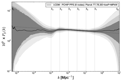
Figure 17: Reconstruction of the marginalized best fit PCHIP PPS (solid line) with 68%, 95% and 99% confidence bands as obtained in the $\Lambda\textrm{CDM}$ model, with the “’Planck TT,TE,EE+lowP+MPkW” dataset, using a PCHIP parameterization with 8 nodes for the PPS. The dotted line represents the power-law PPS corresponding to the Planck best fit Ade et al. (2015b).

X Conclusions

The description of the cosmological model may require a non-standard power-law Primordial Power Spectrum (PPS) of scalar perturbations generated during the inflationary phase at the beginning of the Universe. Several analyses have considered the possible deviations from the PPS power-law exploiting both the WMAP and the Planck data measurements of the CMB temperature power spectrum Shafieloo and Souradeep (2004); Nicholson and Contaldi (2009); Hazra et al. (2013, 2014); Nicholson et al. (2010); Hunt and Sarkar (2014, 2015); Goswami and Prasad (2013); Matsumiya et al. (2002, 2003); Kogo et al. (2004, 2005); Nagata and Yokoyama (2008); Ade et al. (2015a); Gariazzo et al. (2015a); Di Valentino et al. (2015a). Even if the significance for such deviations is small, it leaves some freedom for the PPS assumed form. Here we test the robustness of the cosmological bounds on several cosmological parameters when the PPS is allowed to have a model-independent shape, that we describe using a PCHIP function to interpolate a series of twelve or eight nodes $P_{s,j}$.

We have explored the impact of a non-canonical PPS in several different extensions of the $\Lambda\textrm{CDM}$ model, varying the effective number of relativistic species, the masses of the active and the light sterile neutrinos, the neutrino perturbations and a thermal axion mass.

Concerning the effective number of degrees of freedom $N_{\rm{eff}}$, we find that the results are in good agreement with the standard value of 3.046, if one assumes the standard power-law PPS. Increasing $N_{\rm{eff}}$ has the main effect of increasing the Silk damping of the CMB spectrum at small scales and therefore it is easy change the PPS shape at that scales to compensate the increased damping. This results in a strong degeneracy between the relevant PCHIP PPS nodes and $N_{\rm{eff}}$. As a consequence of volume effects in the Bayesian analyses, the constraints on $N_{\rm{eff}}$ are significantly loosened. For some data combinations we obtain $N_{\rm{eff}}\simeq 4.8$ allowed at 95% CL. However, the PCHIP PPS nodes and $N_{\rm{eff}}$ effects can not be compensated in the polarization spectra, in particular in the case of the TE cross-correlation. This is the reason for which the inclusion of CMB polarization measurements in the analyses allows to break the degeneracies and to restore the $N_{\rm{eff}}$ bounds very close to 3.046 for all the data combinations, with $N_{\rm{eff}}>3.5$ excluded at more than 95% CL for all the datasets.

In the minimal three active massive neutrinos scenario, the constraints on $\Sigma m_{\nu}$ are relaxed with respect to the PPS power-law ones. This is due to the degeneracy between $\Sigma m_{\nu}$ and the nodes $P_{s,5}$ and $P_{s,6}$, that correspond to the scales at which the early Integrated Sachs-Wolfe (eISW) effect contributes to the CMB spectrum. The tightest limit we find is $\Sigma m_{\nu}<0.218$ eV at 95% CL from the combination of Planck TT,TE,EE+lowP+BAO data. The situation is not significantly changed when the effective number and the neutrino masses are varied simultaneously, since the degeneracies with the PPS parameterization are different for these two neutrino parameters. Their constraints are slightly relaxed as a consequence of the increased parameter space. The strongest bounds on $\Sigma m_{\nu}$ arise from the Planck TT,TE,EE+lowP+BAO dataset, for which we obtain $\Sigma m_{\nu}<0.18\,\mathrm{eV}$ (power-law PPS) and $\Sigma m_{\nu}<0.24\,\mathrm{eV}$ (PCHIP PPS). For $N_{\rm{eff}}$, all the data combinations including the Planck CMB polarization measurements give similar constraints, summarized as $2.5\lesssim N_{\rm{eff}}\lesssim 3.5$ at 95% CL.

In the case in which we consider both massive neutrinos and massive sterile neutrino species, the bounds on $\Sigma m_{\nu}$, $m_{s}^{\rm{eff}}$  and $N_{\rm{eff}}$ are weaker for the PCHIP approach when compared to the standard power-law PPS parameterization. This occurs because there exist degeneracies between these parameters and some nodes of the PCHIP PPS. The most stringent constraints on the active and the sterile neutrino parameters are obtained from the combination of Planck TT,TE,EE+lowP+BAO, for which we find $\Sigma m_{\nu}<0.199$ eV, $m_{s}^{\rm{eff}}<0.69$ eV and $N_{\rm{eff}}<3.41$ at 95% CL in the power-law PPS description and $\Sigma m_{\nu}<0.219$ eV, $m_{s}^{\rm{eff}}<0.61$ eV and $N_{\rm{eff}}<3.53$ at 95% CL within the PCHIP PPS parameterization.

Regarding the thermal axion scenario, we notice that the axion mass bounds are largely relaxed when using the PCHIP approach. When including the small scale CMB polarization we find a further weakening of the axion mass constraints: the reduced volume of the posterior distribution for small axion masses ($m_{a}$) is translated into a broadening of the marginalized constraints towards higher values for $m_{a}$. The strongest bound we find on the thermal axion mass within the PCHIP approach is $m_{a}<1.07$ eV at 95% CL when considering the Planck TT+lowP+BAO data combination (while, in the power-law scenario, $m_{a}<0.74$ eV at 95% CL). Finally, when including massive neutrinos in addition to the thermal axions, we find that, while the bounds on the thermal axion mass are unaffected, the constraints on the total neutrino mass are tighter than those obtained without thermal axions. The strongest bounds we find for the thermal axion mass and the total neutrino mass in the PCHIP approach are $m_{a}<1.03$ eV at 95% CL and $\Sigma m_{\nu}<0.180$ eV at 95% CL, when considering the Planck TT+lowP+BAO and Planck TT,TE,EE+lowP+BAO dataset combinations, respectively. In the power-law PPS scenario the strongest bounds are $m_{a}<0.76$ eV at 95% CL and $\Sigma m_{\nu}<0.159$ eV at 95% CL, obtained for the Planck TT,TE,EE+lowP+BAO dataset.

In summary, we have shown that degeneracies among the parameters involved in the $\Lambda\textrm{CDM}$ model (and its possible extensions) and the PPS shape arise when considering CMB temperature power spectrum measurements only. Fortunately, these degeneracies disappear with the inclusion of high-$\ell$ polarization data. This is due to the fact that all these cosmological parameters influence the TT, TE and EE spectra in different ways. This confirms the robustness of both the $\Lambda\textrm{CDM}$ model and the simplest inflationary models, that predict a power-law PPS that successfully explains the observations at small scales. The large scale fluctuations of the CMB spectrum, however, seem to point towards something new in the scenarios that describe inflation. It must be clarified whether these features are indicating a more complicated inflationary mechanism or are instead statistical fluctuations of the CMB temperature anisotropies.

Furthermore, we have as well verified that current data, albeit showing a very mild preference for the power-law scenario, is far from robustly discarding the PCHIP parameterization, and, therefore, future cosmological measurements are mandatory to sharpen the PPS profile.

Appendix A Tables

Parameter	Planck TT+lowP		Planck TT,TE,EE+lowP		Planck TT+lowP		Planck TT,TE,EE+lowP
					+MPkW		+MPkW
$\Omega_{b}h^{2}$	$0.02222\,^{+0.00045}_{-0.00043}$	$0.02175\,^{+0.00077}_{-0.00076}$	$0.02225\,^{+0.00032}_{-0.00030}$	$0.02215\,^{+0.00038}_{-0.00037}$	$0.02221\,^{+0.00044}_{-0.00045}$	$0.02190\,^{+0.00072}_{-0.00070}$	$0.02223\pm 0.00031$	$0.02214\,^{+0.00035}_{-0.00036}$
$\Omega_{c}h^{2}$	$0.1197\,^{+0.0043}_{-0.0042}$	$0.1231\,^{+0.0061}_{-0.0059}$	$0.1198\pm 0.0029$	$0.1209\,^{+0.0035}_{-0.0034}$	$0.1198\pm 0.0039$	$0.1223\,^{+0.0056}_{-0.0053}$	$0.1200\,^{+0.0028}_{-0.0027}$	$0.1210\pm 0.0033$
$100\theta$	$1.0409\pm 0.0009$	$1.0405\pm 0.0011$	$1.0408\pm 0.0006$	$1.0407\pm 0.0006$	$1.0409\,^{+0.0009}_{-0.0010}$	$1.0406\pm 0.0010$	$1.0408\pm 0.0006$	$1.0407\pm 0.0006$
$\tau$	$0.078\,^{+0.038}_{-0.036}$	$0.073\,^{+0.044}_{-0.042}$	$0.079\pm 0.034$	$0.082\pm 0.040$	$0.075\,^{+0.038}_{-0.039}$	$0.076\,^{+0.048}_{-0.046}$	$0.076\,^{+0.034}_{-0.033}$	$0.083\,^{+0.038}_{-0.037}$
$n_{S}$	$0.966\pm 0.012$	–	$0.964\pm 0.010$	–	$0.965\pm 0.011$	–	$0.964\pm 0.009$	–
$\ln[10^{10}A_{s}]$	$3.089\,^{+0.072}_{-0.069}$	–	$3.094\pm 0.066$	–	$3.084\,^{+0.073}_{-0.074}$	–	$3.087\,^{+0.066}_{-0.065}$	–
$H_{0}\,\mathrm{[km\,s^{-1}\,Mpc^{-1}]}$	$67.3\,^{+1.9}_{-1.8}$	$65.7\pm 2.7$	$67.3\pm 1.3$	$66.8\pm 1.5$	$67.3\,^{+1.7}_{-1.8}$	$66.1\pm 2.5$	$67.2\pm 1.2$	$66.7\,^{+1.5}_{-1.4}$
$\sigma_{8}$	$0.83\pm 0.03$	$0.87\pm 0.06$	$0.83\pm 0.03$	$0.88\,^{+0.05}_{-0.06}$	$0.83\pm 0.03$	$0.84\,^{+0.04}_{-0.03}$	$0.83\pm 0.03$	$0.83\pm 0.03$
$P_{s,1}$	$\equiv 1.365$	$<7.93$	$\equiv 1.397$	$<7.69$	$\equiv 1.371$	$<7.90$	$\equiv 1.388$	$<7.68$
$P_{s,2}$	$\equiv 1.140$	$1.15\,^{+0.38}_{-0.35}$	$\equiv 1.155$	$1.14\,^{+0.39}_{-0.36}$	$\equiv 1.139$	$1.14\,^{+0.39}_{-0.36}$	$\equiv 1.147$	$1.14\,^{+0.38}_{-0.36}$
$P_{s,3}$	$\equiv 1.115$	$0.73\,^{+0.39}_{-0.37}$	$\equiv 1.128$	$0.71\,^{+0.38}_{-0.35}$	$\equiv 1.113$	$0.73\,^{+0.39}_{-0.38}$	$\equiv 1.120$	$0.72\,^{+0.38}_{-0.37}$
$P_{s,4}$	$\equiv 1.091$	$1.19\,^{+0.26}_{-0.25}$	$\equiv 1.102$	$1.22\,^{+0.23}_{-0.22}$	$\equiv 1.088$	$1.19\pm 0.25$	$\equiv 1.094$	$1.22\pm 0.22$
$P_{s,5}$	$\equiv 1.067$	$1.07\pm 0.11$	$\equiv 1.076$	$1.08\,^{+0.11}_{-0.10}$	$\equiv 1.063$	$1.07\,^{+0.12}_{-0.11}$	$\equiv 1.069$	$1.08\pm 0.10$
$P_{s,6}$	$\equiv 1.043$	$1.06\,^{+0.09}_{-0.08}$	$\equiv 1.051$	$1.07\,^{+0.08}_{-0.08}$	$\equiv 1.040$	$1.06\pm 0.09$	$\equiv 1.044$	$1.07\,^{+0.08}_{-0.07}$
$P_{s,7}$	$\equiv 1.021$	$1.04\,^{+0.09}_{-0.08}$	$\equiv 1.027$	$1.04\pm 0.08$	$\equiv 1.016$	$1.03\pm 0.09$	$\equiv 1.020$	$1.04\,^{+0.08}_{-0.07}$
$P_{s,8}$	$\equiv 0.998$	$0.99\,^{+0.09}_{-0.08}$	$\equiv 1.003$	$1.01\pm 0.08$	$\equiv 0.993$	$1.00\pm 0.09$	$\equiv 0.996$	$1.01\,^{+0.08}_{-0.07}$
$P_{s,9}$	$\equiv 0.976$	$0.97\,^{+0.09}_{-0.08}$	$\equiv 0.980$	$0.99\,^{+0.08}_{-0.07}$	$\equiv 0.971$	$0.98\pm 0.09$	$\equiv 0.973$	$0.99\,^{+0.08}_{-0.07}$
$P_{s,10}$

References

- Guth (1981) A. H. Guth, Phys. Rev. D23, 347 (1981).
- Linde (1982) A. D. Linde, Phys. Lett. B108, 389 (1982).
- Starobinsky (1982) A. A. Starobinsky, Phys. Lett. B117, 175 (1982).
- Hawking (1982) S. W. Hawking, Phys. Lett. B115, 295 (1982).
- Albrecht and Steinhardt (1982) A. Albrecht and P. J. Steinhardt, Phys. Rev. Lett. 48, 1220 (1982).
- Mukhanov et al. (1992) V. F. Mukhanov, H. A. Feldman, and R. H. Brandenberger, Phys. Rept. 215, 203 (1992).
- Mukhanov and Chibisov (1981) V. F. Mukhanov and G. V. Chibisov, JETP Lett. 33, 532 (1981), [Pisma Zh. Eksp. Teor. Fiz.33,549(1981)].
- Lucchin and Matarrese (1985) F. Lucchin and S. Matarrese, Phys. Rev. D32, 1316 (1985).
- Lyth and Riotto (1999) D. H. Lyth and A. Riotto, Phys. Rept. 314, 1 (1999), hep-ph/9807278 .
- Bassett et al. (2006) B. A. Bassett, S. Tsujikawa, and D. Wands, Rev. Mod. Phys. 78, 537 (2006), astro-ph/0507632 .
- Baumann and Peiris (2009) D. Baumann and H. V. Peiris, Adv. Sci. Lett. 2, 105 (2009), arXiv:0810.3022 [astro-ph] .
- Romano and Cadavid (2014) A. E. Romano and A. G. Cadavid, (2014), arXiv:1404.2985 [astro-ph.CO] .
- Kitazawa and Sagnotti (2014) N. Kitazawa and A. Sagnotti, JCAP 1404, 017 (2014), arXiv:1402.1418 [hep-th] .
- Martin et al. (2014) J. Martin, C. Ringeval, and V. Vennin, Phys. Dark Univ. 5-6, 75 (2014), arXiv:1303.3787 [astro-ph.CO] .
- Chluba et al. (2015) J. Chluba, J. Hamann, and S. P. Patil, Int. J. Mod. Phys. D24, 1530023 (2015), arXiv:1505.01834 [astro-ph.CO] .
- Shafieloo and Souradeep (2004) A. Shafieloo and T. Souradeep, Phys. Rev. D70, 043523 (2004), arXiv:astro-ph/0312174 [astro-ph] .
- Nicholson and Contaldi (2009) G. Nicholson and C. R. Contaldi, JCAP 0907, 011 (2009), arXiv:0903.1106 [astro-ph.CO] .
- Hazra et al. (2013) D. K. Hazra, A. Shafieloo, and T. Souradeep, Phys. Rev. D87, 123528 (2013), arXiv:1303.5336 [astro-ph.CO] .
- Hazra et al. (2014) D. K. Hazra, A. Shafieloo, and T. Souradeep, JCAP 1411, 011 (2014), arXiv:1406.4827 [astro-ph.CO] .
- Nicholson et al. (2010) G. Nicholson, C. R. Contaldi, and P. Paykari, JCAP 1001, 016 (2010), arXiv:0909.5092 [astro-ph.CO] .
- Hunt and Sarkar (2014) P. Hunt and S. Sarkar, JCAP 1401, 025 (2014), arXiv:1308.2317 [astro-ph.CO] .
- Hunt and Sarkar (2015) P. Hunt and S. Sarkar, (2015), arXiv:1510.03338 [astro-ph.CO] .
- Goswami and Prasad (2013) G. Goswami and J. Prasad, Phys. Rev. D88, 023522 (2013), arXiv:1303.4747 [astro-ph.CO] .
- Matsumiya et al. (2002) M. Matsumiya, M. Sasaki, and J. Yokoyama, Phys. Rev. D65, 083007 (2002), arXiv:astro-ph/0111549 [astro-ph] .
- Matsumiya et al. (2003) M. Matsumiya, M. Sasaki, and J. Yokoyama, JCAP 0302, 003 (2003), arXiv:astro-ph/0210365 [astro-ph] .
- Kogo et al. (2004) N. Kogo, M. Matsumiya, M. Sasaki, and J. Yokoyama, Astrophys. J. 607, 32 (2004), arXiv:astro-ph/0309662 [astro-ph] .
- Kogo et al. (2005) N. Kogo, M. Sasaki, and J. Yokoyama, Prog. Theor. Phys. 114, 555 (2005), arXiv:astro-ph/0504471 [astro-ph] .
- Nagata and Yokoyama (2008) R. Nagata and J. Yokoyama, Phys. Rev. D78, 123002 (2008), arXiv:0809.4537 [astro-ph] .
- Ade et al. (2015a) P. A. R. Ade et al. (Planck Collaboration), (2015a), arXiv:1502.02114 [astro-ph.CO] .
- Bennett et al. (2013) C. L. Bennett et al. (WMAP), Astrophys. J. Suppl. 208, 20 (2013), arXiv:1212.5225 [astro-ph.CO] .
- Ade et al. (2014a) P. A. R. Ade et al., Astron. Astrophys. 571, A1 (2014a), arXiv:1303.5062 .
- Adam et al. (2015) R. Adam et al., (2015), 1502.01582 .
- de Putter et al. (2014) R. de Putter, E. V. Linder, and A. Mishra, Phys. Rev. D89, 103502 (2014), arXiv:1401.7022 [astro-ph.CO] .
- Gariazzo et al. (2015a) S. Gariazzo, C. Giunti, and M. Laveder, JCAP 1504, 023 (2015a), arXiv:1412.7405 [astro-ph.CO] .
- Di Valentino et al. (2015a) E. Di Valentino, S. Gariazzo, E. Giusarma, and O. Mena, Phys. Rev. D91, 123505 (2015a), arXiv:1503.00911 [astro-ph.CO] .
- Gariazzo et al. (2015b) S. Gariazzo, L. Lopez-Honorez, and O. Mena, Phys. Rev. D92, 063510 (2015b), arXiv:1506.05251 [astro-ph.CO] .
- Lewis et al. (2000) A. Lewis, A. Challinor, and A. Lasenby, Astrophys. J. 538, 473 (2000), astro-ph/9911177 .
- Lewis and Bridle (2002) A. Lewis and S. Bridle, Phys. Rev. D66, 103511 (2002), astro-ph/0205436 .
- Ade et al. (2015b) P. A. R. Ade et al., (2015b), 1502.01589 .
- Mangano et al. (2005) G. Mangano, G. Miele, S. Pastor, T. Pinto, O. Pisanti, and P. D. Serpico, Nucl. Phys. B729, 221 (2005), hep-ph/0506164 .
- Fritsch and Carlson (1980) F. Fritsch and R. Carlson, SIAM Journal on Numerical Analysis 17, 238 (1980).
- Fritsch and Butland (1984) F. Fritsch and J. Butland, SIAM Journal on Scientific and Statistical Computing 5, 300 (1984).
- Aghanim et al. (2015) N. Aghanim et al., Submitted to: Astron. Astrophys. (2015), 1507.02704 .
- Beutler et al. (2011) F. Beutler, C. Blake, M. Colless, D. H. Jones, L. Staveley-Smith, L. Campbell, Q. Parker, W. Saunders, and F. Watson, Mon. Not. Roy. Astron. Soc. 416, 3017 (2011), arXiv:1106.3366 [astro-ph.CO] .
- Ross et al. (2015) A. J. Ross, L. Samushia, C. Howlett, W. J. Percival, A. Burden, and M. Manera, Mon. Not. Roy. Astron. Soc. 449, 835 (2015), arXiv:1409.3242 [astro-ph.CO] .
- Anderson et al. (2014) L. Anderson et al. (BOSS), Mon. Not. Roy. Astron. Soc. 441, 24 (2014), arXiv:1312.4877 [astro-ph.CO] .
- Parkinson et al. (2012) D. Parkinson et al., Phys. Rev. D86, 103518 (2012), arXiv:1210.2130 [astro-ph.CO] .
- Ade et al. (2015c) P. A. R. Ade et al., (2015c), 1502.01591 .
- Hou et al. (2013) Z. Hou, R. Keisler, L. Knox, M. Millea, and C. Reichardt, Phys. Rev. D87, 083008 (2013), arXiv:1104.2333 [astro-ph.CO] .
- Lesgourgues et al. (2013) J. Lesgourgues, G. Mangano, G. Miele, and S. Pastor, Neutrino Cosmology (Cambridge University Press, 2013) iSBN: 9781139012874.
- Archidiacono et al. (2013a) M. Archidiacono, E. Giusarma, S. Hannestad, and O. Mena, Adv. High Energy Phys. 2013, 191047 (2013a), 1307.0637 [astro-ph] .
- Gariazzo et al. (2015c) S. Gariazzo, C. Giunti, M. Laveder, Y. F. Li, and E. M. Zavanin, (2015c), arXiv:1507.08204 [hep-ph] .
- Reid et al. (2010) B. A. Reid, L. Verde, R. Jimenez, and O. Mena, JCAP 1001, 003 (2010), arXiv:0910.0008 .
- Hamann et al. (2010) J. Hamann, S. Hannestad, J. Lesgourgues, C. Rampf, and Y. Y. Y. Wong, JCAP 1007, 022 (2010), arXiv:1003.3999 [astro-ph.CO] .
- de Putter et al. (2012) R. de Putter et al., Astrophys. J. 761, 12 (2012), arXiv:1201.1909 [astro-ph.CO] .
- Giusarma et al. (2013a) E. Giusarma, R. De Putter, and O. Mena, Phys. Rev. D87, 043515 (2013a), arXiv:1211.2154 [astro-ph.CO] .
- Zhao et al. (2013) G.-B. Zhao et al., Mon. Not. Roy. Astron. Soc. 436, 2038 (2013), arXiv:1211.3741 [astro-ph.CO] .
- Hou et al. (2014) Z. Hou et al., Astrophys. J. 782, 74 (2014), arXiv:1212.6267 [astro-ph.CO] .
- Archidiacono et al. (2013b) M. Archidiacono, E. Giusarma, A. Melchiorri, and O. Mena, Phys. Rev. D87, 103519 (2013b), arXiv:1303.0143 [astro-ph.CO] .
- Giusarma et al. (2013b) E. Giusarma, R. de Putter, S. Ho, and O. Mena, Phys. Rev. D88, 063515 (2013b), arXiv:1306.5544 [astro-ph.CO] .
- Riemer-Sørensen et al. (2014) S. Riemer-Sørensen, D. Parkinson, and T. M. Davis, Phys. Rev. D89, 103505 (2014), arXiv:1306.4153 [astro-ph.CO] .
- Hu et al. (2014) J.-W. Hu, R.-G. Cai, Z.-K. Guo, and B. Hu, JCAP 1405, 020 (2014), arXiv:1401.0717 [astro-ph.CO] .
- Giusarma et al. (2014) E. Giusarma, E. Di Valentino, M. Lattanzi, A. Melchiorri, and O. Mena, Phys. Rev. D90, 043507 (2014), arXiv:1403.4852 [astro-ph.CO] .
- Di Valentino et al. (2015b) E. Di Valentino, E. Giusarma, O. Mena, A. Melchiorri, and J. Silk, (2015b), arXiv:1511.00975 [astro-ph.CO] .
- Ade et al. (2014b) P. A. R. Ade et al., Astron. Astrophys. 571, A16 (2014b), arXiv:1303.5076 [astro-ph.CO] .
- Abazajian et al. (2012) K. N. Abazajian et al., (2012), 1204.5379 [hep-ph] .
- Kopp et al. (2013) J. Kopp, P. A. N. Machado, M. Maltoni, and T. Schwetz, JHEP 05, 050 (2013), 1303.3011 [hep-ph] .
- Gonzalez-Garcia et al. (2015) M. C. Gonzalez-Garcia, M. Maltoni, and T. Schwetz, (2015), arXiv:1512.06856 [hep-ph] .
- Peccei and Quinn (1977a) R. D. Peccei and H. R. Quinn, Phys. Rev. Lett. 38, 1440 (1977a).
- Peccei and Quinn (1977b) R. D. Peccei and H. R. Quinn, Phys. Rev. D16, 1791 (1977b).
- Weinberg (1978) S. Weinberg, Phys. Rev. Lett. 40, 223 (1978).
- Wilczek (1978) F. Wilczek, Phys. Rev. Lett. 40, 279 (1978).
- Olive et al. (2014) K. A. Olive et al. (Particle Data Group), Chin. Phys. C38, 090001 (2014).
- Archidiacono et al. (2015) M. Archidiacono, T. Basse, J. Hamann, S. Hannestad, G. Raffelt, and Y. Y. Y. Wong, JCAP 1505, 050 (2015), arXiv:1502.03325 [astro-ph.CO] .
- Melchiorri et al. (2007) A. Melchiorri, O. Mena, and A. Slosar, Phys. Rev. D76, 041303 (2007), arXiv:0705.2695 [astro-ph] .
- Hannestad et al. (2007) S. Hannestad, A. Mirizzi, G. G. Raffelt, and Y. Y. Y. Wong, JCAP 0708, 015 (2007), arXiv:0706.4198 [astro-ph] .
- Hannestad et al. (2008) S. Hannestad, A. Mirizzi, G. G. Raffelt, and Y. Y. Y. Wong, JCAP 0804, 019 (2008), arXiv:0803.1585 [astro-ph] .
- Hannestad et al. (2010) S. Hannestad, A. Mirizzi, G. G. Raffelt, and Y. Y. Y. Wong, JCAP 1008, 001 (2010), arXiv:1004.0695 [astro-ph.CO] .
- Archidiacono et al. (2013c) M. Archidiacono, S. Hannestad, A. Mirizzi, G. Raffelt, and Y. Y. Y. Wong, JCAP 1310, 020 (2013c), arXiv:1307.0615 [astro-ph.CO] .
- Di Valentino et al. (2015c) E. Di Valentino, E. Giusarma, M. Lattanzi, O. Mena, A. Melchiorri, and J. Silk, (2015c), arXiv:1507.08665 [astro-ph.CO] .
- Di Valentino et al. (2015d) E. Di Valentino, A. Melchiorri, and J. Silk, Phys. Rev. D92, 121302 (2015d), arXiv:1507.06646 [astro-ph.CO] .