QFix: Diagnosing errors through query histories
Abstract
Data-driven applications rely on the correctness of their data to function properly and effectively. Errors in data can be incredibly costly and disruptive, leading to loss of revenue, incorrect conclusions, and misguided policy decisions. While data cleaning tools can purge datasets of many errors before the data is used, applications and users interacting with the data can introduce new errors. Subsequent valid updates can obscure these errors and propagate them through the dataset causing more discrepancies. Even when some of these discrepancies are discovered, they are often corrected superficially, on a case-by-case basis, further obscuring the true underlying cause, and making detection of the remaining errors harder.
In this paper, we propose QFix, a framework that derives explanations and repairs for discrepancies in relational data, by analyzing the effect of queries that operated on the data and identifying potential mistakes in those queries. QFix is flexible, handling scenarios where only a subset of the true discrepancies is known, and robust to different types of update workloads. We make four important contributions: (a) we formalize the problem of diagnosing the causes of data errors based on the queries that operated on and introduced errors to a dataset; (b) we develop exact methods for deriving diagnoses and fixes for identified errors using state-of-the-art tools; (c) we present several optimization techniques that improve our basic approach without compromising accuracy, and (d) we leverage a tradeoff between accuracy and performance to scale diagnosis to large datasets and query logs, while achieving near-optimal results. We demonstrate the effectiveness of QFix through extensive evaluation over benchmark and synthetic data.
1 Introduction
Poor data quality is a hard and persistent problem. It is estimated to cost the US economy more than $600 billion per year [17] and erroneous price data in retail databases alone cost the US consumers $2.5 billion each year [18]. Although data cleaning tools can purge many errors from a dataset before downstream applications use the data, datasets can frequently change as applications and users execute queries that modify the data. Mistakes in these queries can introduce errors to the data, and these errors can propagate to more data by subsequent update queries. By the time errors are detected, their origin has often been obscured and it is difficult to identify the offending query and correct it. Identifying and correcting errors in the data directly is suboptimal, as it targets the symptom, rather than the underlying cause. Fixing the manifested data errors on a case-by-case basis often obscures the root of the problem and other data that may have been affected. Therefore, traditional data cleaning approaches are not well-suited for this setting: While they provide general-purpose tools to identify and rectify anomalies in the data, they are not designed to diagnose the causes of errors that are rooted in erroneous updates. Some data cleaning systems try to identify structural sources of mistakes [35], but they are unable to trace the source of the mistakes to particular faulty queries.
While improving data quality and correcting data errors has been an important focus for data management research, handling new errors, introduced during regular database interactions, has received little attention. Most work in this direction focuses on guarding against erroneous updates. For example, integrity constraints [27] reject some improper updates, but only if the data falls outside rigid, predefined ranges. Certificate-based verification [7] is less rigid, but it is impractical and non-scalable as it requires users to answer challenge questions before allowing the updates, and it is not applicable to updates initiated by applications.
In this paper, we present QFix, a diagnosis and repair framework for data errors caused by erroneous updates. In contrast to existing approaches in data cleaning that aim to detect and correct errors in the data directly, the goal of QFix is to identify errors in the queries that introduced errors in the data. These diagnoses explain how errors were introduced to a dataset, and allow an administrator to easily identify and further validate the most likely query-based sources of these errors. In addition, once the erroneous queries have been confirmed, repairing the source of the errors can potentially lead to the identification of additional discrepancies in the data that would have otherwise remained undetected. We describe two motivating examples; the first is a real-life scenario, provided to us by a large US-based wireless provider.
Example 1 (Wireless discount policies)
A wireless provider offers company discounts as incentives for corporate customers. There are different types of discounts (flat, percentage, fee-based), and their details are specific to corporate agreements. The large number of policies and complexities in their rules frequently cause policies to be set incorrectly, leading to errors in the application of discounts to customers’ accounts.
Customers who notice billing errors contact the provider, but the call centers do not have the capacity or ability to investigate the complaints deeply. The standard course of action is to correct mistakes on a case-by-case basis for each complaint. As a result, unreported errors remain in the database for a long time, or they never get corrected, and their cause becomes harder to trace as further queries modify the database.
Example 2 (Tax bracket adjustment)
Tax brackets determine tax rates for different income levels and are often adjusted. Accounting firms implement these changes to their databases by appropriately updating the tax rates of their customers. Mistakes in these update queries (e.g., Figure 2) result in errors in the tax rates and computed taxes.
In these application scenarios, data errors are typically reported to a customer service department, which does not have the resources nor the capability to investigate the errors more broadly. Instead, errors are resolved on a case-by-case basis. The goal of QFix is to identify the query or queries that caused the errors and propose corrections to those queries. Once these repairs have been validated (say, by an expert), they can be used to identify unreported errors and to prevent the introduction of more errors. This problem has the following important characteristics that render it very difficult, and unsuitable for traditional techniques:
- Obscurity.
-
Handling data errors directly often leads to partial fixes that further complicate the eventual diagnosis and resolution of the problem. For example, a transaction implementing a change in the state tax law updated tax rates using the wrong rate, affecting a large number of consumers. This causes a large number of complaints to a call center, but each customer agent usually fixes each problem individually, which ends up obscuring the source of the problem.
- Large impact.
-
Erroneous queries cause errors at a large scale. The potential impact of the errors is high, as manifested in several real-world cases [39, 24, 32]. Further, errors that remain undetected for a significant amount of time can instigate additional errors, even through valid updates. This increases both their impact, and their obscurity.
- Systemic errors.
-
The errors created by bad queries are systemic: they have common characteristics, as they share the same cause. The link between the resulting data errors is the query that created them; cleaning techniques should leverage this connection to diagnose and fix the problem. Diagnosing the cause of the errors, will achieve systematic fixes that will correct all relevant errors, even if they have not been explicitly identified.
QFix does not replace traditional data cleaning methods, but rather, complements them. Instead of identifying errors in the data directly, QFix targets the diagnosis, explanation, and repair of errors at the root by leveraging example errors acquired from users, traditional data cleaning, or detection techniques.
Diagnosing data errors stemming from incorrect updates is fundamentally challenging: the search space of possible mistakes and fixes is large, and the amount of information (number of known errors) may be limited. QFix addresses these challenges by analyzing the queries that operated on a dataset in an efficient and scalable manner. More concretely, we make the following contributions:
-
•
We formalize the problem of diagnosing a set of errors using log histories of updates that operated on the data. Given a set of complaints as representations of data discrepancies in the current state of a dataset, QFix determines how to resolve all of the complaints with the minimal amount of changes to the queries in the log (Section 3).
-
•
We provide an exact error-diagnosis solution through a non-trivial transformation of the problem to a mixed integer linear program (MILP) that encodes the data provenance of the erroneous tuples. Our approach employs state-of-the-art MILP solvers to identify optimal diagnoses that are guaranteed to resolve all complaints without introducing new errors to the data (Section 4).
-
•
We present several optimizations to our basic diagnostic method, which reduce the problem size without affecting the quality of the produced solutions. Further, we propose an incremental repair method that targets the cases where the log contains a single corrupted query (or the search focuses on a single repair). This incremental analysis of the log allows us to scale to large datasets ( records) and large query logs (hundreds to thousands of update queries). Further, we show that our optimization techniques have the additional advantage of tolerating incomplete information, such as unreported errors (Section 5).
-
•
We perform a thorough evaluation of the trade-offs between speed and accuracy of our baseline and optimized methods under a controlled, synthetic setting. In particular, we demonstrate that the QFix optimizations achieve significant speedup compared to the baseline algorithm (40 in some of our experimental settings). We also evaluate QFix on common OLTP benchmarks and show how QFix can propose fully accurate repairs within milliseconds on a TPC-C workload with queries (Section 7).
To the best of our knowledge, QFix is the first system that diagnoses and repairs errors through query histories. We show that it is extremely effective and efficient with the update workloads found in most common benchmarks. While QFix trusts its input to be correct, it can handle incomplete information, and it can be resilient to some inaccuracies in the reported data errors (Section 6). QFix does not handle some complex query types that are less common in update workloads, such as nested queries, joins, and aggregation. It also does not currently deal with large amounts of incorrect information, such as fake data errors reported by malicious users. These challenges present exciting future extensions to the system presented in this work.
2 QFix System Architecture
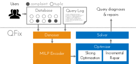
Figure 1 shows the QFix architecture. The system takes two inputs: a log of update queries (including UPDATE, INSERT, and DELETE statements) and a set of identified data errors (complaints). QFix analyzes the data errors and the query logs to trace the causes of the errors in queries in the log (diagnoses), and to automatically derive query repairs. The query repairs represent corrections to the queries in the log, and can be used to identify additional errors in the data that were not reported.
The core of QFix is the MILP Encoder, which expresses the query diagnosis problem as a Mixed Integer Linear Program (MILP), and the constraint problem is solved by the Solver. The Optimizer uses slicing and incremental techniques that help the system scale to large datasets and query logs efficiently, while maintaining high accuracy. For completeness, an optional Denoiser can be applied to the inputs to detect and remove incorrect complaints—we regard this component as orthogonal to this paper.
3 Modeling abstractions
In this section, we introduce a running example inspired from the use-case of Example 2, and describe the model abstractions that we use to formalize the diagnosis problem.
| Taxes: | |||
|---|---|---|---|
| ID | income | owed | pay |
| $9500 | $950 | $8550 | |
| $90000 | $22500 | $67500 | |
| $86000 | $21500 | $64500 | |
| $86500 | $21625 | $64875 | |
| Query log: | |
|---|---|
| : | UPDATE Taxes SET owed=income*0.3 |
| WHERE income>=85700 | |
| : | INSERT INTO Taxes |
| VALUES (25, 85800, 21450) | |
| : | UPDATE Taxes SET pay=income-owed |
| Taxes: | |||
|---|---|---|---|
| ID | income | owed | pay |
| $9500 | $950 | $8550 | |
| $90000 | $27000 | $63000 | |
| $86000 | $25800 | $60200 | |
| $86500 | $25950 | $60550 | |
| $87000 | $21750 | $65250 | |
Example 3
Figure 2 demonstrates an example tax bracket adjustment in the spirit of Example 2. The adjustment sets the tax rate to 30% for income levels above $87,500, and is implemented by query . A digit transposition mistake in the query, results in an incorrect owed amount for tuples and . Query , which inserts a tuple with slightly higher income than and and the correct information, obscures this mistake. This mistake is further propagated by query , which calculates the pay check amount based on the corresponding income and owed.
While traditional data cleaning techniques seek to identify and correct the erroneous values in the table Taxes directly, our goal is to diagnose the problem, and understand the reasons for these errors. In this case, the reason for the data errors is the incorrect predicate value in query .
In this paper, we assume that we know some errors in the dataset, and that these errors were caused by erroneous updates. The errors may be obtained in different ways: traditional data cleaning tools may identify discrepancies in the data (e.g., a tuple with lower income has higher owed tax amount), or errors can be reported directly from users (e.g., customers reporting discrepancies to customer service). Our goal is not to correct the errors directly in the data, but to analyze them as a “symptom” and provide a diagnosis. The diagnosis can produce a targeted treatment: knowing how the errors were introduced guides the proper way to trace and resolve them.
| Notation | Description |
|---|---|
| The sequence of executed update queries (log) | |
| Initial database state at beginning of log | |
| End database state (current) | |
| Database state after query : | |
| Complaint: | |
| Complaint set | |
| Modifier function of (e.g., SET clause) | |
| Conditional function of (e.g., WHERE clause) | |
| Tuple values introduced in an INSERT query | |
| Log repair | |
| Distance functions between two query logs |
3.1 Error Modeling
In our setting, the diagnoses are associated with errors in the queries that operated on the data. In Example 3, the errors in the dataset are due to the digit transposition mistake in the WHERE clause predicate of query . Our goal is to infer the errors in a log of queries automatically, given a set of incorrect values in the data. We proceed to describe our modeling abstractions for data, queries, and errors, and how we use them to define the diagnosis problem.
Data and query models
Query log (): We define a query log that update the database as an ordered sequence of UPDATE, INSERT, and DELETE queries , that have operated on a database . In the rest of the paper, we use the term update queries, or just queries, to refer to any of the queries in , including insertion and deletion queries.
Query (): We model each query as a function over a database , resulting in a new database . For INSERT queries, . We model UPDATE and DELETE queries as follows:
In this definition, the modifier function represents the query’s update equations, and it transforms a tuple by either deleting it () or changing the values of some of its attributes. The conditional function is a boolean function that represents the query’s condition predicates. In the example of Figure 2:
Note that in this paper, we only consider query without sub-query or aggregation.
Database state (): We use to represent the state of a database after the application of queries through from the log . represents the original database state, and the final, or current, database state. Out of all the states, the system only maintains and . In practice, can be a checkpoint: a state of the database that we assume is correct; we cannot diagnose errors before this state. The intermediate states can be derived by executing the log: . We also write to denote that the final database state can be derived by applying the sequence of queries in the log to the original database state .
True database state (): Queries in are possibly erroneous, introducing errors in the data. There exists a sequence of true database states , with , representing the database states that would have occurred if there had been no errors in the queries. The true database states are unknown; our goal is to find and correct the errors in and retrieve the correct database state .
For ease of exposition, in the remainder of the paper we assume that the database contains a single relation with attributes , but the single table is not a requirement in our framework.
Error models
Following the terminology in Examples 1 and 2, we model a set of identified or user-reported data errors as complaints. A complaint corresponds to a particular tuple in the final database state , and identifies that tuple’s correct value assignment. We formally define complaints below:
Definition 4 (Complaint)
A complaint is a mapping between two tuples: , such that and have the same schema, , and . A complaint defines a transformation on a database state : .
In the example of Figure 2, two complaints are reported on the final database state : and , where and . For both these cases, each complaint denotes a value correction for a tuple in . Complaints can also model the addition or removal of tuples: means that should be added to the database, whereas means that should be removed from the database.
Complaint set (): We use to denote the set of all known complaints , and we call it the complaint set. Each complaint in represents a transformation (addition, deletion, or modification) of a tuple in . We assume that the complaint set is consistent, i.e., there are no two complaints that propose different transformations to the same tuple . Applying all these transformations to results in a new database instance .111Since the complaint set is consistent, it is easy to see that the order of transformations is inconsequential. is complete if it contains a complaint for each error in . In that case, . In our work, we do not assume that the complaint set is complete, but, as is more common in practice, we only know a subset of the errors (incomplete complaint set). Further, we focus our analysis on valid complaints; we briefly discuss dealing with invalid complaints (complaints identifying a correct value as an error) in Section 6, but these techniques are beyond the scope of this paper.
Log repair (): The goal of our framework is to derive a diagnosis as a log repair , such that . In this work, we focus on errors produced by incorrect parameters in queries, so our repairs focus on altering query constants rather than query structure. Therefore, for each query , has the same structure as (e.g., the same number of predicates and the same variables in the WHERE clause), but possibly different parameters. For example, a good log repair for the example of Figure 2 is , where =UPDATE Taxes SET owed=income*0.3 WHERE income >= 87500.
Problem definition
We now formalize the problem definition for diagnosing data errors using query logs. A diagnosis is a log repair that resolves all complaints in the set and leads to a correct database state .
Definition 5 (Optimal diagnosis)
Given database states and , a query log such that , a set of complaints on , and a distance function , the optimal diagnosis is a log repair , such that:
-
•
, where has no errors
-
•
is minimized
More informally, we seek the minimum changes to the log that would result in a clean database state . Obviously, a challenge is that is unknown, unless we know that the complaint set is complete.
Problem scope and solution outline
In this work, we assume basic data manipulation queries with no subqueries, aggregations, or joins; these operations are not as common in update workloads. QFix supports queries with WHERE clauses containing conjunctions and disjunctions of predicates. Predicates and SET expressions can be over linear combinations of constants and attributes. We study the impact of the number of predicates in the WHERE clause in Section 7.3.
In Section 4, we describe our basic method, which uses a constraint programming formulation that expresses this diagnosis problem as a mixed integer linear program (MILP). Section 5 presents several optimization techniques that extend the basic method, allowing QFix to (1) handle cases of incomplete information (incomplete complaint set), and (2) scale to large data and log sizes. Specifically, the fully optimized, incremental algorithm (Section 5.4), can handle query logs with hundreds of queries within minutes, while the performance of the basic approach collapses by queries.
Due to space considerations, we omit discussion of alternative approaches that use classification tools and linear systems of equations. These approaches are limited to a query log containing a single query, and are discussed and evaluated in more detail in our technical report [36].
4 A MILP-based Solution
In this section, we introduce a basic solver-based approach to resolve the errors reflected in the complaint set. This approach constructs a mixed-integer linear programming (MILP) problem by linearizing and parameterizing the corrupted query log over the tuples in the database. Briefly, an MILP is a linear program where only a subset of the undetermined variables are required to be integers, while the rest are real-valued.
Our general strategy is to model each query as a linear equation that computes the output tuple values from the inputs and to transform the equation into a set of of linear constraints. In addition, the constant values in the queries are parameterized into a set of undetermined variables, while the database state is encoded as constraints on the initial and final tuple values. Finally, the undetermined variables are used to construct an objective function that prefers value assignments that minimize both the amount that the queries change and the number of non-complaint tuples that are affected.
The rest of this section will first describe the process of linearizing a single query and translating it into a set of constraints. We then extend the process to the entire query log and finally define the objective function. Subsequent sections introduce optimizations that both improve the speed and quality of the results, as well as harness the trade-off between the two.
4.1 Encoding a Single Query
MILP problems express constraints as a set of linear inequalities. Our task is to derive such a mathematical representation for each query in . Starting with the functional representation of a query (Section 3.1), we describe how each query type, UPDATE, INSERT, and DELETE, can be transformed into a set of linear constraints over a tuple and an attribute value .
UPDATE: Recall from Section 3.1 that query can be modeled as the combination of a modifier function and conditional function . First, we introduce a binary variable to indicate whether satisfies the conditional function of : if and otherwise. In a slight abuse of notation:
| (1) |
Next, we introduce real-valued variables for the attributes of . We express the updated value of an attribute using semi-modules, borrowing from the models of provenance for aggregate operations [2]. A semi-module consists of a commutative semi-ring, whose elements are scalars, a commutative monoid whose elements are vectors, and a multiplication-by-scalars operation that takes a scalar and a vector and returns a vector . A similar formalism has been used in literature to model hypothetical data updates [29].
Given a query and tuple , we express the value of attribute in the updated tuple as follows:
| (2) |
In this expression, the operation corresponds to regular multiplication, but we maintain the notation to indicate that it is a semi-module multiplication by scalars. This expression models the action of the update: If satisfies the conditional function (), then takes the value ; if does not satisfy the conditional function (), then takes the value . In our running example, the rate value of a tuple after query would be expressed as: . Equation (2) does not yet provide a linear representation of the corresponding constraint, as it contains multiplication of variables. To linearize this expression, we adapt a method from [29]: We introduce two variables and to represent the two terms of Equation (2): and . Assuming a number as the upper bound of the domain of , we get the following constraints:
| (3) | ||||||
The set of conditions on ensure that if , and otherwise. Similarly, the conditions on ensure that if , and otherwise. Now, Equation (2) becomes linear:
| (4) |
INSERT:An insert query adds a new tuple to the database. If the query were corrupted, then the inserted values need repair. We use a binary variable to model whether the query is correct. Each attribute of the newly inserted tuple () may take one of two values: the value specified by the insertion query () if the query is correct (), or an undetermined value () if the query is incorrect (). Thus, similar with Equation (2), we write:
| (5) |
DELETE: A delete query removes a set of tuples from the database. Since the MILP problem doesn’t have a way to express a non-existent value, we encode a deleted tuple by setting its attributes to a value outside of the attribute domain . In this way, subsequent conditional functions on the attribute will return false, so it will not have an effect on subsequent queries encoded in the MILP problem:
| (6) | |||||
This expression is further linearized using the same method as Equation (4.1).
Putting it all together. The constraints defined in Equations (1)–(6) form the main structure of the MILP problem for a single attribute of a single tuple . To linearize a query one needs to apply this procedure to all attributes and tuples. This process is denoted as in Algorithm 1. Our MILP formulation includes three types of variables: the binary variables , the real-valued attribute values (e.g., ), and the real-valued constants in and . All these variables are undetermined and need to be assigned values by a MILP solver.
Next, we extend this encoding to the entire query log, and incorporate an objective function encouraging solutions that minimize the overall changes to the query log.
4.2 Encoding and Repairing the Query Log
We proceed to describe the procedure (Algorithm 1) that encodes the full query log into a MILP problem, and solves the MILP problem to derive . The algorithm takes as input the query log , the initial and final (dirty) database states , and the complaint set , and outputs a fixed query log .
We first call Linearize on each tuple in and each query in , and add the result to a set of constraints milp_cons. The function AssignVals adds constraints to set the values of the inputs to and the outputs of to their respective values in and . Additional constraints account for the fact that the output of query is the input of (ConnectQueries). This function simply equates from the linearized result for to the input for the linearized result of .
Finally, EncodeObjective augments the program with an objective function that models the distance function between the original query log and the log repair (). In the following section we describe our model for the distance function, though other models are also possible. Once the MILP solver returns a variable assignment, ConvertQLog updates the constants in the query log based on this assignment, and constructs the fixed query log .
4.3 The Objective Function
The optimal diagnosis problem (Definition 5) seeks a log repair , such that the distance is minimized. In this section, we describe our model for the objective function, which assumes numerical parameters and attributes. This assumption is not a restriction of the QFix framework. Handling other data types, such as categorical values comes down to defining an appropriate distance function, which can then be directly incorporated into QFix.
In our experiments, we use the normalized Manhattan distance (in linearized format in the MILP problem) between the parameters in and . We use to denote the parameter of query , and to denote the total number of parameters in :
Different choices for the objective function are also possible. For example, one may prioritize the total number of changes incurred in the log, rather than the magnitude of these changes. However, a thorough investigation of different possible distance metrics is beyond the scope of our work.
5 Optimizing the Basic Approach
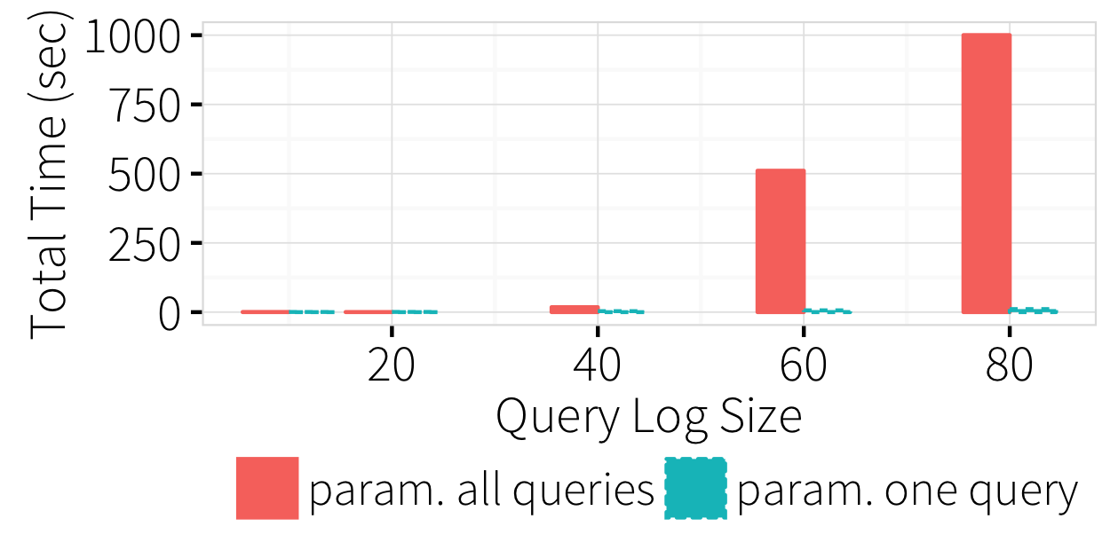
A major drawback of our basic MILP transformation (Section 4) is that it exhaustively encodes the combination of all tuples in the database and all queries in the query log. In this approach, the number of constraints (as well as undetermined variables) grows quadratically with respect to the database and the query log. This increase has a large impact on the running time of the solver, since it needs to find a (near)-optimal assignment of all undetermined variables (exponential with the number of undetermined variables). This is depicted in Figure 4, which increases the query log size over a database of tuples. The red bars encode the problem using the basic algorithm that parameterizes all queries, while the blue bars show the potential gain of only parameterising the oldest query that we assume is incorrect. At a log size of , the solver for basic failed to produce an answer within seconds. Although MILP solvers exhibit empirical performance variation, this experiment illustrates the performance limitation of the basic approach.
A second limitation of basic is its inability to handle errors in the complaint set. This is because the basic MILP formulation generates hard constraints for all of the database records, thus any error, whether a false negative missing complaint or a false positive incorrect complaint, must be correct. It may be impossible to find a repair that satisfies this condition and will lead to solver infeasibility errors.
The rest of this section describes three classes of slicing optimizations that reduce the number of tuples, queries, and attributes that are encoded in the MILP problem. The tuple-slicing technique additionally improves the repair accuracy when the complaint set is incomplete. We also propose an incremental algorithm that avoids the exponential increase in solver time by only parameterizing a small number of queries at a time—thus limiting the cost to the left side of Figure 4.
5.1 Tuple Slicing: Reducing Tuples
Our first optimization, tuple-slicing, applies a two step process to reduce the problem size without sacrificing accuracy: it first aggressively reduces the problem size by only encoding tuples in the complaint set and then refines the log repair through a second but much smaller MILP problem.
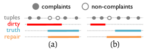
Step 1 (Initial Repair Step): The first step of tuple slicing aggressively reduces the problem size by only encoding those tuples in the complaint set (Algorithm 1 line is replaced with for each t in ). Each tuple necessitates the linearization of the entire query log, thus, only encoding the complaint tuples minimizes the size of the problem with respect to the relevant tuples. This optimization is guaranteed to resolve , thus depending on the properties of the non-complaint records, it can generate correct repairs an order of magnitude faster without hurting the accuracy. In Figure 5(a), the solver will guarantee a repair interval that excludes the two left-most complaints, includes the two right-most complaints, and minimizes the difference between the dirty and repaired intervals (due to the objective function). This effectively pushes the repair’s lower-bound towards that of the dirty interval. This is a case where such a solution is correct, because the dirty and truth intervals overlap. Recall that we do not have access to the truth interval, and our goal is to reproduce the truth interval given (solid circles) and the corrupted query.
However, this approach can also cause the repair to be a superset of the truth interval, and affect tuples not part of the complaint set. Figure 5(b) highlights such a case where the dirty and truth intervals are non-overlapping, and the non-complaint record between them has been incorrectly included in the repair interval—because the MILP problem did not include the non-complaint.
In both of these cases, the objective function will ensure that the repair does not over-generalize the upper bound towards the right because that strictly increases the objective function. Therefore, our main concern is to refine the repair interval to exclude those non-complaint tuples in case (b). Note that in the case of incomplete complaint sets, the user may opt to no execute the refinement step if she believes that the non-complaint records are indeed in error.
Step 2 (Refinement Step): Although there are many possible mechanisms to refine the initial repair (e.g., incrementally shrinking the repaired interval until the non-complaint tuples are all excluded), the straightforward approaches are not effective when multiple corrupt queries have been repaired because they don’t take the query interactions into account.
Instead, we solve this with a second, significantly smaller, MILP problem. Let be the set of repaired queries from the initial MILP formulation with tuple slicing; be the set of non-complaint tuples now matching the repaired WHERE clauses, as in Figure 5(b); and . We create a new MILP using as the complaint set. The key is to only parameterize the repaired clauses from Step 1 as constraints with undetermined variables. The variables for all other tuples and queries are fixed to their assigned values from Step 1. This refines the solutions from the previous step while incorporating knowledge about complaints in , Finally, we use a new objective function to minimize the number of non-complaint tuples that are matched by the solution.
In our experiments, we find that this second MILP iteration adds minimal overhead () with respect to the initial MILP problem. In summary, tuple-slicing is an effective method to improve the performance of the basic approach, without compromising, and often improving, repair quality.
5.2 Query Slicing: Reducing Queries
In practice, many of the queries in the query log could not have affected the complaint attributes (defined below). For example, if and only read and wrote attribute , then they could not have contributed to an error in . However, if wrote , then either or both queries may have caused the error. In short, if we model a query as a set of attribute read and write operations, those not part of the causal read-write chain to the complaint attributes can be ignored. This is the foundation of our query-slicing optimization.
Definition 6 (Complaint Attributes )
The set of attributes identified as incorrect in the complaint set.
Definition 7 (Query dependency & impact)
Query has direct-impact, , which is the set of attributes updated in its modifier function (e.g., SET clause). Its dependency, , is the set of attributes involved in its condition function . We derive the full-impact, , of a query by propagating its direct impact through subsequent queries in the log (Algorithm 2):
By computing the full-impact of , we can determine the extent that it affects based on its overlap with the complaint attributes. Specifically, when , may affect all complaint attributes and is a candidate for repair; when , contributed to a subset of the complaint attributes and is a candidate for repair; when , is irrelevant and can be ignored during the repair process. We distinguish between the first and second conditions in the special case where we are repairing a single corrupted query in the query log. In this case, only queries in the first conditions are candidates for repair because the single query must have caused errors in all of the complaint attributes. This enables QFix to scale significantly better for this important problem setting. Finally, we use to denote the set of relevant queries that are candidates for repair. Our query slicing optimization linearizes only the queries in , rather than the entire log, resulting in smaller problems than the basic approach without any loss of accuracy.
5.3 Attribute Slicing: Reducing Attributes
In addition to removing irrelevant queries, we additionally avoid encoding irrelevant attributes. Given , the relevant attributes can be defined as: We propose attribute slicing optimization that only encodes constraints for attributes in . We find that this type of slicing can be effective for wide tables along with queries that focus on a small subset of attributes.
5.4 Incremental Repairs
Even with the slicing optimizations, the number of undetermined variables can remain high, resulting in slow solver runtime. The red bars in Figure 4 showed the exponential cost of parameterizing the entire query log as compared to only solving for a single query (blue bars). These results suggest that it is faster to run many small MILP problems than a single large one, and motivates our incremental algorithm.
Our approach (Algorithm 3) focuses on the case where there is a single corrupted query to repair. It does so by linearizing the full query log, including any slicing optimizations, but only parameterizing and repairing a batch of consecutive queries at a time. This procedure first attempts to repair the most recent queries, and continues to the next queries if a repair was not generated. The algorithm internally calls a modified version of the basic approach that takes extra parameters , only parameterizes those queries, and fixes the values of all other variables.
The incremental approach prioritizes repairs for complaints that are due to more recent corruptions. Given that the basic algorithm simply fails beyond a small log size, we believe this is a natural and pragmatic assumption to use, and results in a scalability improvement. Our experiments further evaluate different batching level in the incremental algorithm and show that it is impractical from both a performance and accuracy to have .
6 Noisy Complaint Sets
As described in the problem setup (Section 3.1), complaint sets may be imperfect. First, complaint sets are typically incomplete, missing errors that occur in , but are not reported. In this case, the naive encoding of the query log and database (basic) will likely produce an infeasible MILP. In the running example of Figure 2, if the complaint set is incomplete and only contains a complaint on , basic will interpret as a correct state and repairing the condition of to a value greater than will appear to introduce a new error. The solver will declare the problem infeasible and will not return a solution.
However, the tuple slicing optimization (Section 5.1) implicitly corrects this problem: By only encoding the tuples in the incomplete complaint set, the encoded problem does not enforce constraints on the query’s effect on other tuples in the database. This allows the result to generalize to tuples not in the complaint set. The second iteration of the MILP execution then uses a soft constraint on the number of non-complaint tuples that are affected by the repair in order to address the possibility of over-generalization.
Another possible inaccuracy in the complaint set is the presence of false positives: some complaints may be incorrectly reporting errors, or the target tuple of a complaint may be incorrect. This type of noise in the complaint set can also lead to infeasibility. One can remove such erroneous complaints as a pre-processing step, using one of numerous outlier detection algorithms. While this is an interesting problem, it is orthogonal to the query repair problem that we are investigating in this work. Thus, in our experiments, we focus on incomplete complaints sets and assume that there are not erroneous complaints.
7 Experiments
In this section, we carefully study the performance and accuracy characteristics of the basic MILP-based repair algorithm, slicing-based optimizations that improve the latency of the system, and the incremental algorithm for single query corruptions. Due to the difficulty of collecting corrupt query logs from active deployments, our goal instead is to understand these trade-offs in controlled synthetic scenarios, as well as study the effectiveness in typical database query workloads based on widely used benchmarks.
To this end, our experiments are organized as follows: First, we compare the basic and incremental MILP algorithm against the different optimizations to highlight the value of different optimizations and the limitations of the basic approach. We then show that UPDATE queries are particularly difficult to repair and focus solely on different types of UPDATE-only workloads to understand how QFix responds to different parameter settings. We end with an evaluation using established database transaction benchmarks from OLTP-bench [15]: TPC-C [11] and TATP [37]. All experiments were run on 12x2.66 GHz machines with 16GB RAM running IBM CPLEX [12] as the MILP solver on CentOS release 6.6.
7.1 Experimental Setup
For each of our experiments we generate and corrupt a query log. We execute the original and corrupt query logs on an initial (possibly empty) database, perform a tuple-wise comparison between the resulting database states to generate a true complaint set, and simulate incomplete complaint sets by removing a subset of the true complaints. Finally, we execute the algorithms and compare the repaired query log with the true query log, as well as the repaired and true final database states, to measure performance and accuracy metrics. Performance is measured as wall clock time between submitting a complaint set and the system terminating after retrieving a valid repair. Accuracy is measured as the repair’s precision (percentage of repaired tuples that were correctly fixed), the recall (the percentage of the full complaint set that was repaired), and the F1 measure (the harmonic mean of precision and recall). We report the average across 20 runs. We describe the experimental parameters in the context of the datasets and workloads below.
Synthetic: We generate an initial database of random tuples. The schema contains a primary key along with attributes , whose values are integers picked from uniformly at random. We then generate a sequence of queries. The default setting for these parameters are: .
UPDATE queries are defined by a SET clause that assigns an attribute a or value, and a WHERE clause can either be a predicate on a key, or a predicate on non-key attributes:
SET Clause: WHERE Clause: Constant: SET (a_i=?), .. Point: WHERE a_j=? & .. Relative: SET (a_i=a_i+?) Range: WHERE a_j in [?,?+r] & ..
where ? is random and r is the size of the range predicate.
Query selectivity is by default (r).
Note that a range predicate where r = 0 is distinct from a predicate due to the non-key attribute.
The WHERE clauses in DELETE queries are generated in an identical fashion, while
INSERT queries insert values picked uniformly at random from .
By default, we generate UPDATE queries with non-key range predicates and constant set clauses.
In addition, the skew parameter determines the distribution attributes referenced in the WHERE and SET clauses. Each attribute in a query is picked from either a uniform distribution when or a zipfian distribution with exponent . This allows our experiments to vary between a uniform distribution, where each attribute is equally likely to be picked, and a skewed distribution where nearly all attributes are the same.
Benchmarks: We use the TPC-C [11] and TATP [37] benchmarks. The former generates the ORDER table at scale 1 with one warehouse, and uses the queries that modify the ORDER table. We execute a log of 2000 queries over an initial table containing 6000 tuples. queries are INSERTs and the rest are UPDATEs. The latter TATP workload simulates the caller location system. We generate a database from SUBSCRIBER table with 5000 tuples and UPDATE queries. Both setups were generated using the OLTP-bench [15]. We introduce a single corruption, and vary corrupted query’s index from the most recent query to .
Corrupting Queries: We corrupt query by replacing it with a randomly generated query of the same type based on the procedures described above. To standardize our procedures, we selected a fixed set of indexes that are used in all experiments.
7.2 Preliminary Analysis
The following set of experiments are designed to establish the rationale for the settings in the subsequent experiments. Specifically, we compare different slicing-based optimizations of basic as the number of queries increases. We then evaluate the scalability of the different slicing-based optimizations of the incremental approach in the context of a single corrupted query. We then establish the difficulty of repairing UPDATE workloads as compared to other query types.
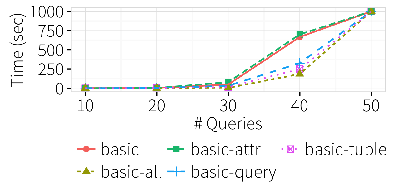
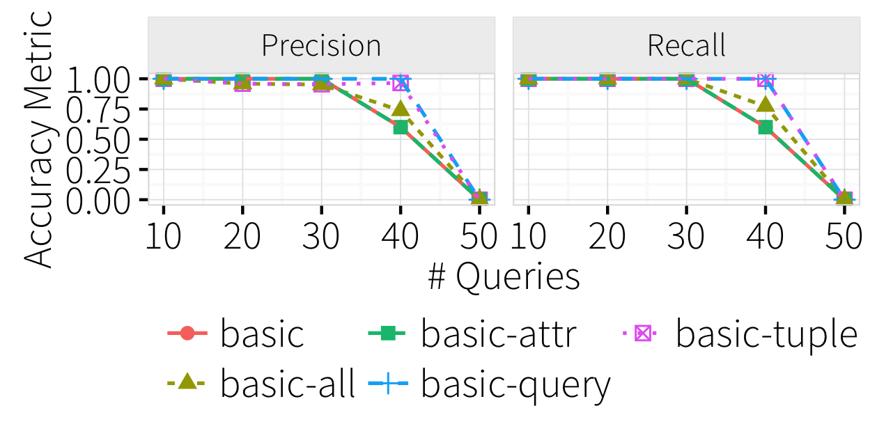
Multiple Corrupt Queries: In this experiment, we compare the basic approach (basic) against each slicing optimization individually() and all of them together (). We use the default settings with tuples and a sequence of UPDATE queries. We generate query logs in 5 different sizes and corrupt every tenth query starting from oldest query , up to . For example, when the , we corrupt 3 queries: . We find that the number of queries greatly affects both the scalabality (Figure 6(a)) and the accuracy (Figure 6(d)) of the algorithms. Specifically, as the number increases, the number of possible assignments of the MILP parameters increases exponentially and the solver often takes longer than our experimental time limit of seconds and returns an infeasibility error. This is a predominant reason why the accuracy degrades past queries. For example, when queries are involved (with corruptions) and we ignore the infeasible executions, the average execution time is seconds and the precision and recall are greater than . Unfortunately, with queries ( corruptions), all runs exceed the time limit and return infeasibility.
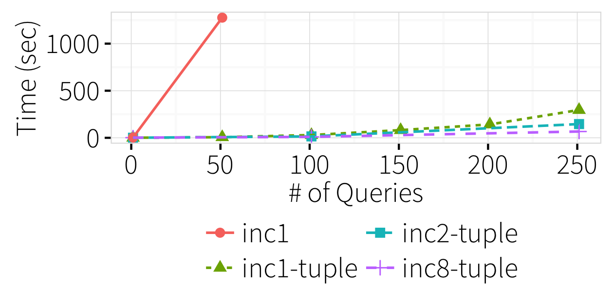
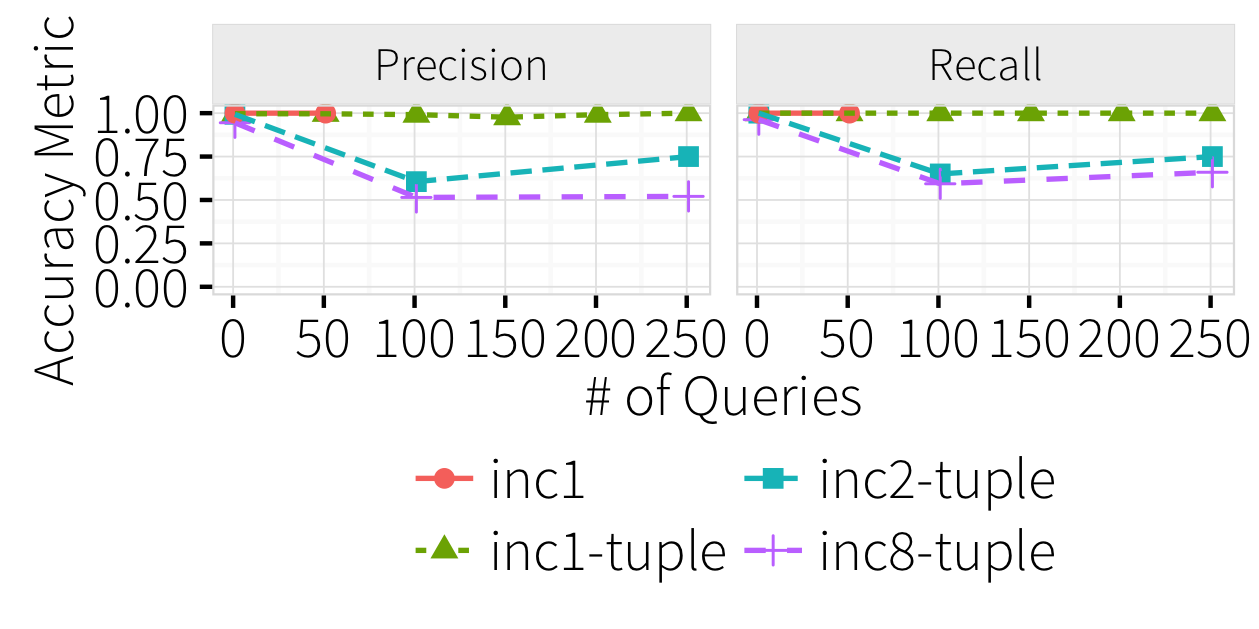
Single Corrupt Query: In this experiment, we evaluate the efficacy QFix with tuple slicing and incremental optimization in the special case when one query has been corrupted in a much larger query log. We compare QFix-inc without tuple slicing () against tuple slicing at different batching levels of 1, 2, 8 (). Recall from Section 5.4 that parameterizes consecutive queries in each batch until a repair is found. Figure 6(b) highlights the scalability limitation of the incremental algorithm without tuple-slicing: with 50 queries easily exceeds the 1000s limit. The tuple-slicing scales significantly better (nearly faster), however the accuracy severely degrades when . The primary reason is because of infeasibility errors—the MILP problem is much harder, and fails to find a repair. This is highlighted by the symmetry between the precision and recall curves. A secondary reason is beause the refinement step of tuple slicing may not generate a fully correct repair and generalize incorrectly. This is why the precision curve is lower than the recall curve for .
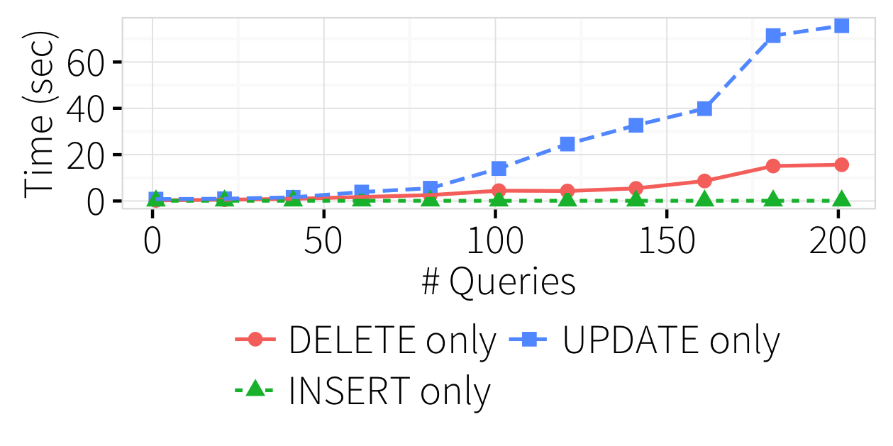
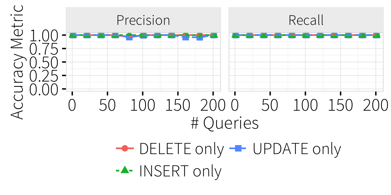
Query Type: Our final preliminary experiment evaluates the incremental algorithm with tuple slicing optimization () on INSERT, DELETE, or UPDATE-only workloads. We increase the number of queries from to and corrupt the oldest query in the log. Figure 6(c) shows that while the cost of repairing INSERT workloads remains relatively constant, the cost for DELETE-only and UPDATE-only workloads increase as the corruption happens earlier in the query log—and a much faster rate for UPDATE queries. The F1 score for all settings is nearly 1 (Figure 6(f)).


Takeaways: We find that basic, even with slicing optimizations, has severe scalability limitations due to the large number of undetermined values—this is unsurprising as MILP constraint solving is an NP-hard problem. In contrast, the incremental algorithms can scale to larger query log sizes, however only a batch size of can retain high repair quality. UPDATE queries translate into more undetermined variables than other query types, and are significantly more expensive to repair. Based on these results, we focus on the incremental algorithm and the more difficult UPDATE-only workloads.
7.3 Synthetic Incremental Experiments
We divide these experiments into two groups: the first evaluates the different slicing optimizations under different settings; the latter algorithm and varies workload and dataset parameters. Note that omit accuracy figures when the F1-score is .
Comparing optimizations.
Varying # Attributes: We first evaluate QFix and its optimizations by increasing the number of attribute () with . As shown in Figure 7(a), when the number of attribute in a table is small (e.g., ) all algorithms appear identical. However, increasing the number of attribute exhibits a larger benefit for query and attribute slicing (up to reduction compared to tuple-slicing). When the table is wide (), applying all optimizations () is faster than tuple-slicing alone.
Database Size: We vary the database size () with a large number of attributes (). We fix the number of complaints by decreasing the query selectivity in proportion to ’s increase—the specific mechanism to do so does not affect the findings. Figure 7(b) shows that the costs are relatively flat until the corruption occurs in an old query (). In addition, we find that the cost is highly correlated with the number of candidate queries that are encoded in the MILP problem. The increase in cost despite tuple-slicing is due to the increasing number of candidate queries in the system; we believe this increasing trend is due to the solver’s ability to prune constraints that correspond to queries that clearly will not affect the complaint set—an implicit form of query slicing. Applying attribute-slicing supercedes this implicit optimization and results in a flat curve, while query-slicing explicitly reduces the number of candidate queries in proportion with the database size, and leads to the increasing trend. Ultimately, combining all three optimizations improves the latency over tuple-slicing by in the worst case, and up to in the best case.
Sensitivity to data and workload factors.
The following set of synthetic experiments focus on a single QFix setting—incremental with tuple-slicing—and individually vary numerous database and workload parameters in order to tease apart the algorithm performance. These include factors such as query complexity, log size , database size and the skew of the query predicates. We focus on a narrow table setting that contains attributes, and a single corrupt query in the query log.
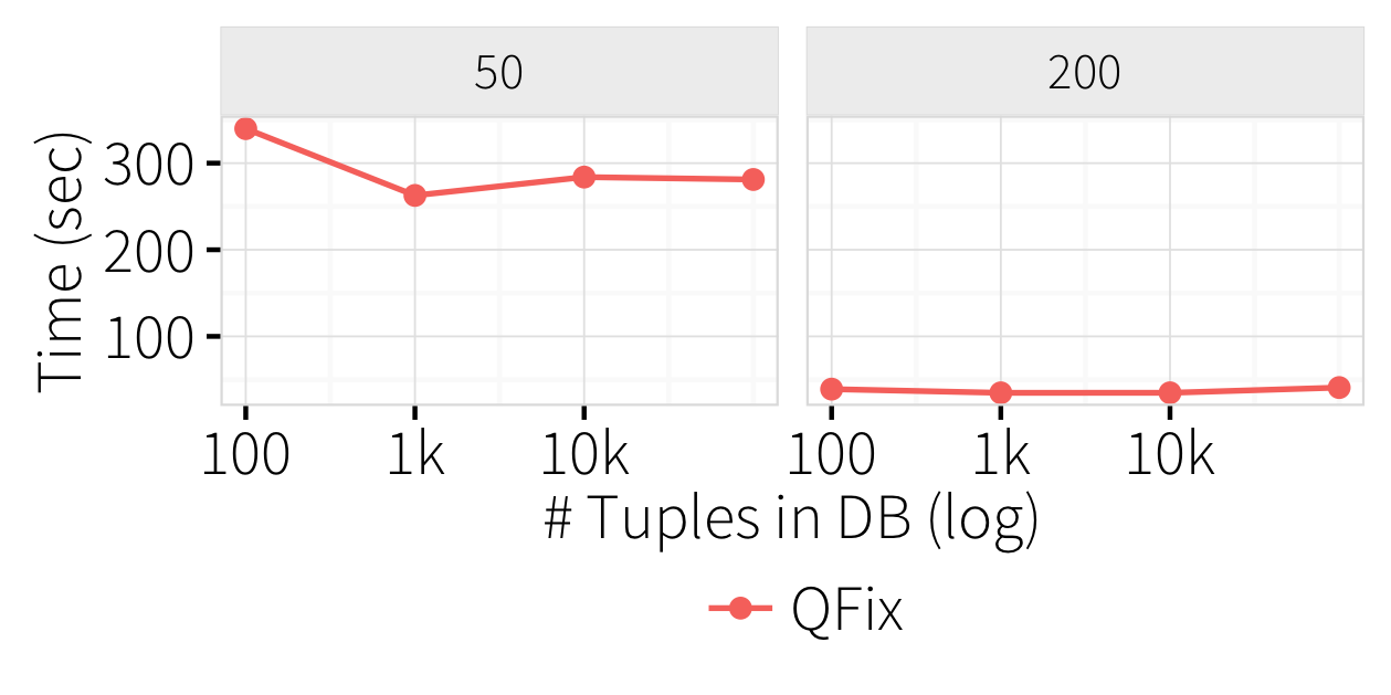
Database Size: Figure 8(a) varies the database size (), and fixes query output cardinality and complaint set size in the same way as the previous scalability experiment. In contrast to the previous experiment, the scalabality curve is nearly flat for both corruption query indices. The reason is because the solver’s implicit pruning optimization is less effective when there are only attributes: Every query is likely to touch an attribute that affects the complaint set. We verified this by applyng query-slicing to the same setting, and found far fewer queries were pruned compared to the previous experiment. It takes less than a minute to perfectly repair the recent corruption , and around minutes for the older corruption , even as the database size increases. At smaller database sizes, the randomness in the workload generator leads to variability in the size of the complaint set, and ultimately a larger and more difficult MILP problem. The exponential relationship between solver time and problem difficulty results in the higher average latency for .
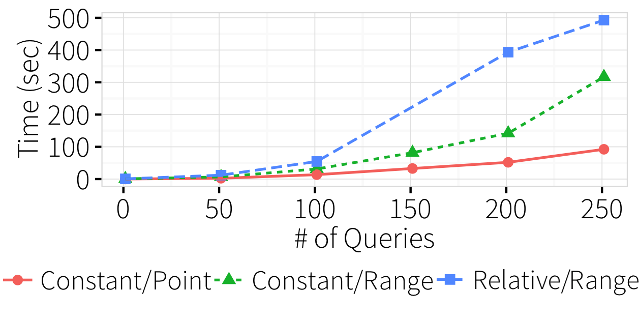
Query Clause Type: So far, we have focused on UPDATE queries with constant set clauses and range predicates. Figure 8(b) individually varies each clause and compares against Constant/Point and Relative/Range queries. The x-axis varies the index of the corrupted query between and . We find that point predicates and constant set clauses are easier to solve than range predicates and relative set clauses, respectively. The reason for the former pair is because range predicates double the number of undetermined variables as compared to point queries. In addition, point queries are on key attributes, thus further reduces the possible search space. We believe the latter pair is because the constant set clauses break the causal relationship between input and output records for the overwritten values. This both simplifies the difficulty of the constraint problem, and reduces the total number of constraints.
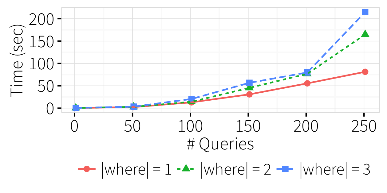
Predicate Dimensionality: Figure 8(e) varies the dimensionality of the update queries by increasing the number of predicates in the WHERE clause, while keeping the query cardinality constant. The cost increases with the dimensionality because each additional predicate is translated into a new set of constraints and undetermined variables, increasing the problem complexity.
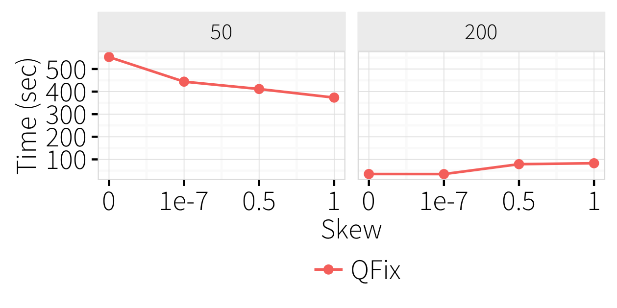
Skew: We now study the effects of attribute skew on the algorithms. We increase the skew parameter from (uniform) to (nearly every attribute is ) and find a reduction in latency (Figure 8(d)). We believe the reason is because increasing the skew focuses the query predicates over a smaller set of logical attributes, and increases the number of constraints placed on each of the logical attributes used in the query log. Each of these constraints reduces the search space of allowable values for that attribute, and thus simplifies the MILP problem. This result suggests that QFix may be well suited for many transaction systems that naturally exhibit query skew. Note that the overall number of constraints in the problem is the same, only their distribution over the query attributes has changed.
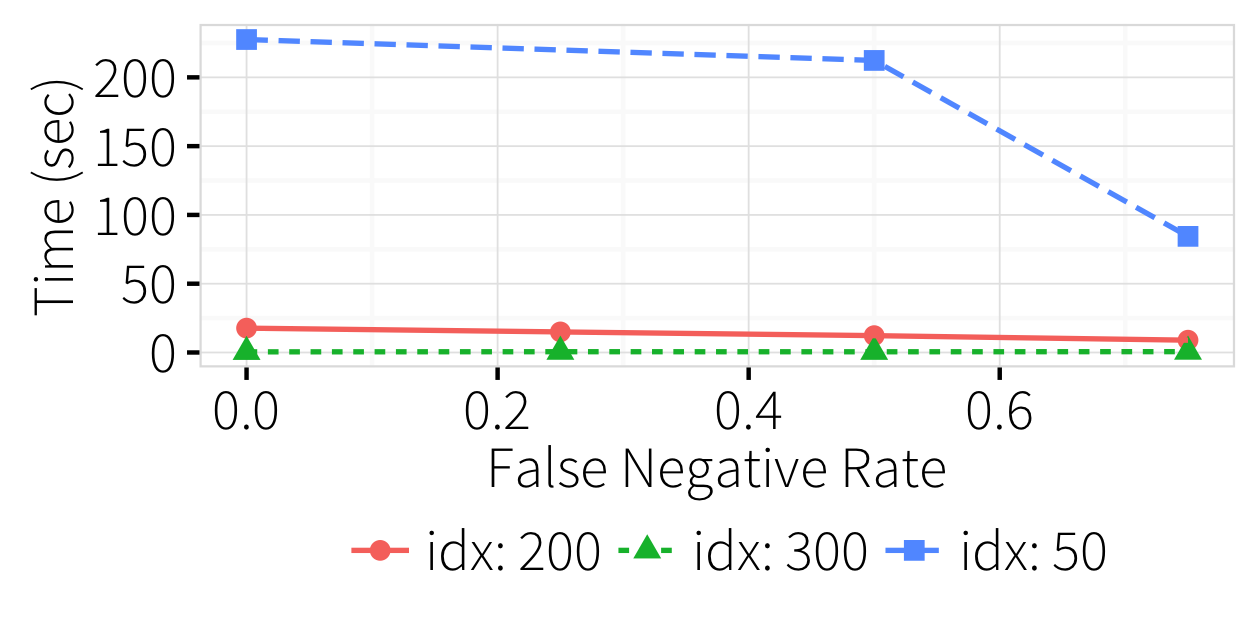
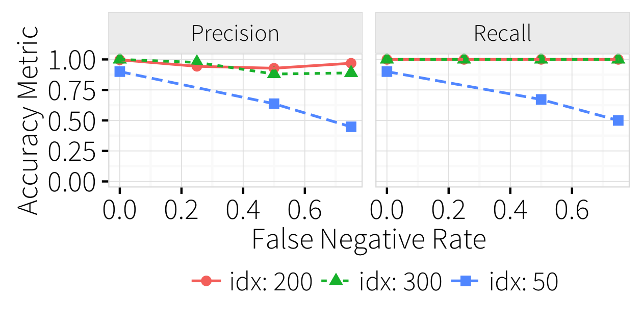
Incomplete Complaint Set: Our final experiment (Figures 8(c) and 8(f)) varies the fase positive rate in incomplete complaint sets. We increase the rate from ( missing in the complaint set) to ( are missing). We find that reducing the size of the submitted complaint set naturally improves the repair performance, however the repair quality, both precision and recall in Figure 8(f), may suffer if the corruption occured in a very old query. This is expected because QFix targets reported complaints, thus unreported complaints may easily be missed and lead to low recall. In addition, despite the refinement step of tuple-slicing, the repair may over generalize and “fix” the wrong records, leading to low precision.
Takeaways: we find that the performance of the different repair algorithm heavily depends on the property of the datasets and queries—in particular, the number of encoded candidate queries and the number of attributes. Attribute and query slicing show significant gain for datasets with large number of attributes. QFix is able to solve hard problems (with UPDATE-only queries) in seconds or minutes—particularly if the error is recent.
7.4 Benchmarks
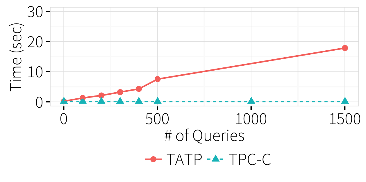
Figure 9 plots the performance of the incremental algorithm using tuple-slicing on the TPC-C and TATP benchmark applications. The key reason is that each query affects a small set of records and leads to a very small complaint set— or on average. In addition, tuple and query slicing can aggressively reduce the total number of constraints to a very small number—often less than in total. Furthermore for TPC-C, the queries are predominantly INSERT queries, which QFix can solve within milliseconds. Finally, we evaluated QFix on Example 2 in Figure 2 and fully repaired the correct query in 35 milliseconds.
Takeaways: many workloads in practice are dominated by INSERT and point UPDATE queries (ignoring the dominant percentage of read-only queries). In these settings, QFix is very effective at reducing the number of constraints and can derive repairs with near-interactive latencies.
8 Related Work
QFix tackles the problem of diagnosis and repair in relational query histories (query logs). It does not aim to correct errors in the data directly, but rather to find the underlying reason for reported errors in the queries that operated on the data. This contrasts with traditional data cleaning [14, 1, 28, 21] which oftentimes focuses on identifying and correcting data “in-place.” as well as cleaning techniques that provide repairs for the identified errors [19, 9, 3, 10, 5]. By analyzing the process that generate the errors, QFix can help detect and repair systemic errors that have not been explicitly identified.
Several tools [23, 35] explore systemic reasons for errors and generate feature sets or patterns of attributes that characterize those errors. However, such techniques are oblivious to the actual executed queries and do not provide fixes.
The topic of query revisions has been studied in the context of why-not explanations [6, 33, 34] and explaining query ouputs [38, 22, 31]. But all these approaches are limited to selection predicates of SELECT queries, and they only typically consider one query at a time.
Finally, as QFix traces errors in the queries that manipulate data, it has connections to the field of data and workflow provenance. our algorithms build on several formalisms introduced by work in this domain. These formalisms express why a particular data item appears in a query result, or how that query result was produced in relation to input data [4, 25, 8, 13].
9 Summary and discussion
The general problem of data errors is highly complex, and exacerbated by its highly contextual nature. We believe that an approach that explains and repairs such data errors based on operations performed by the application or user is a promising step towards incorporating contextual hints into the analysis process.
Towards this goal, we presented QFix, the first framework to diagnose and repair errors in the queries that operate on the data. Datasets are typically dynamic: even if a dataset starts clean, updates may introduce new errors. QFix can analyze query logs to trace reported errors to the queries that introduced them. This in turn helps identify additional errors in the data that may have been missed and gone unreported.
We proposed a basic algorithm, basic, that uses non-trivial transformation rules to encode information from the data and the query log as a MILP problem. We further improve basic with two types of optimizations: (1) slicing-based optimizations that reduce the problem size without compromising the accuracy, but rather often improving it, and (2) an incremental approach that analyzes a single query at a time. Our experiments show that the latter optimization can achieve significant scaling gains for single-query errors, without significant reduction in accuracy.
To the best of our knowledge, QFix is the first formalization and solution to the diagnosis and repair of errors using past executed queries. Obviously, correcting such errors in practice poses additional challenges. The initial version of QFix described in this paper focuses on a constrained problem consisting of simple (no subqueries, UDFs, aggregations, nor joins) single-query transactions with clauses composed of linear functions, and complaint sets without false positives. In future work, we hope to extend our techniques to relax these limitations. In addition, we plan to investigate additional methods of scaling the constraint analysis, as well as techniques that can adapt the benefits of single-query analysis to errors in multiple queries.
References
- [1] S. Abiteboul, S. Cluet, T. Milo, P. Mogilevsky, J. Siméon, and S. Zohar. Tools for data translation and integration. In IEEE Data Engineering Bulletin, 1999.
- [2] Y. Amsterdamer, S. B. Davidson, D. Deutch, T. Milo, J. Stoyanovich, and V. Tannen. Putting lipstick on pig: Enabling database-style workflow provenance. In PVLDB, 2011.
- [3] G. Beskales, I. F. Ilyas, and L. Golab. Sampling the repairs of functional dependency violations under hard constraints. In PVLDB, 2010.
- [4] P. Buneman, S. Khanna, and W. C. Tan. Why and where: A characterization of data provenance. In ICDT, 2001.
- [5] A. Chalamalla, I. F. Ilyas, M. Ouzzani, and P. Papotti. Descriptive and prescriptive data cleaning. In SIGMOD, 2014.
- [6] A. Chapman and H. V. Jagadish. Why not? In SIGMOD, 2009.
- [7] S. Chen, X. L. Dong, L. V. Lakshmanan, and D. Srivastava. We challenge you to certify your updates. In SIGMOD, 2011.
- [8] J. Cheney, L. Chiticariu, and W. C. Tan. Provenance in databases: Why, how, and where. In Foundations and Trends in Databases, 2009.
- [9] X. Chu, I. F. Ilyas, and P. Papotti. Holistic data cleaning: Putting violations into context. In ICDE, 2013.
- [10] G. Cong, W. Fan, F. Geerts, X. Jia, and S. Ma. Improving data quality: Consistency and accuracy. In VLDB, 2007.
- [11] T. T. P. Council. Benchmark c: Standard specification (revision 5.9.0), 2014.
- [12] I. CPLEX. High-performance software for mathematical programming and optimization, 2005.
- [13] Y. Cui, J. Widom, and J. L. Wiener. Tracing the lineage of view data in a warehousing environment. In ACM Transactions on Database Systems, 2000.
- [14] M. Dallachiesa, A. Ebaid, A. Eldawy, A. Elmagarmid, I. F. Ilyas, M. Ouzzani, and N. Tang. Nadeef: a commodity data cleaning system. In SIGMOD, 2013.
- [15] D. E. Difallah, A. Pavlo, C. Curino, and P. Cudre-Mauroux. Oltp-bench: An extensible testbed for benchmarking relational databases. In VLDB, 2013.
- [16] D. E. Difallah, A. Pavlo, C. Curino, and P. Cudre-Mauroux. Oltp-bench: An extensible testbed for benchmarking relational databases. In VLDB, 2013.
- [17] W. W. Eckerson. Data quality and the bottom line. TDWI Report, The Data Warehouse Institute, 2002.
- [18] W. Fan, F. Geerts, and X. Jia. A revival of integrity constraints for data cleaning. In VLDB, 2008.
- [19] W. Fan, F. Geerts, X. Jia, and A. Kementsietsidis. Conditional functional dependencies for capturing data inconsistencies. In ACM Transactions on Database Systems, 2008.
- [20] M. Galar, A. Fernandez, E. Barrenechea, H. Bustince, and F. Herrera. A review on ensembles for the class imbalance problem: bagging-, boosting-, and hybrid-based approaches. Systems, Man, and Cybernetics, Part C: Applications and Reviews, IEEE Transactions on, 42(4):463–484, 2012.
- [21] H. Galhardas, D. Florescu, D. Shasha, and E. Simon. Ajax: An extensible data cleaning tool. In SIGMOD, 2000.
- [22] K. E. Gebaly, P. Agrawal, L. Golab, F. Korn, and D. Srivastava. Interpretable and informative explanations of outcomes. In PVLDB, 2014.
- [23] L. Golab, H. J. Karloff, F. Korn, and D. Srivastava. Data auditor: Exploring data quality and semantics using pattern tableaux. In PVLDB, 2010.
- [24] B. Grady. Oakland unified makes $7.6M accounting error in budget; asking schools not to count on it. In Oakland, 2013.
- [25] T. J. Green, G. Karvounarakis, and V. Tannen. Provenance semirings. In PODS, 2007.
- [26] H. He and E. A. Garcia. Learning from imbalanced data. Knowledge and Data Engineering, IEEE Transactions on, 21(9):1263–1284, 2009.
- [27] N. Khoussainova, M. Balazinska, and D. Suciu. Towards correcting input data errors probabilistically using integrity constraints. In MobiDE, 2006.
- [28] N. Koudas, S. Sarawagi, and D. Srivastava. Record linkage: Similarity measures and algorithms. In SIGMOD, 2006.
- [29] A. Meliou and D. Suciu. Tiresias: The database oracle for how-to queries. In SIGMOD, 2012.
- [30] J. R. Quinlan. Simplifying decision trees. International journal of man-machine studies, 27(3):221–234, 1987.
- [31] S. Roy and D. Suciu. A formal approach to finding explanations for database queries. In SIGMOD, 2014.
- [32] M. Sakal and L. Raković. Errors in building and using electronic tables: Financial consequences and minimisation techniques. In Strategic Management, 2012.
- [33] Q. T. Tran and C.-Y. Chan. How to conquer why-not questions. In SIGMOD, 2010.
- [34] K. Tzompanaki, N. Bidoit, and M. Herschel. Semi-automatic sql debugging and fixing to solve the missing-answers problem. In VLDB PhD Workshop.
- [35] X. Wang, X. L. Dong, and A. Meliou. Data x-ray: A diagnostic tool for data errors. In SIGMOD, 2015.
- [36] X. Wang, A. Meliou, and E. Wu. Qfix: Diagnosing errors through query histories. CoRR, abs/1601.07539, 2016.
- [37] A. Wolski. Tatp benchmark description (version 1.0), 2009.
- [38] E. Wu and S. Madden. Scorpion: Explaining away outliers in aggregate queries. In PVLDB, 2013.
- [39] J. Yates. Data entry error wipes out life insurance coverage. In Chicago Tribune, 2005.
Appendix A A Learning-based Approach
A drawback of the MILP approach is that the generated models grow with the size of the database and query log. However, we argue that the encoded information is necessary in order to generate a sufficient set of constraints that result in a good repair. In this section, we examine an alternative, simpler, decision tree-based approach called DecTree. We show that even in a simple case of a single query log and a complete complaint set, it is expected to perform poorly. We will first describe how to model the repair process using a decision tree, and then we will present and discuss experimental results that illustrate its limitations.
A.1 Modeling Repairs with Decision Trees
Rule-based learners are used in classification tasks to generate a set of rules, or conjunctive predicates that best classify a group of labeled tuples. The rules are non-overlapping, and each is associated with a label—a tuple that matches a given rule is assigned the corresponding label. These rules exhibit a natural parallel with SQL WHERE clauses, which can be viewed as labeling selected tuples with a positive label and rejected tuples with a negative label. Similarly, the structure of the rules is identical to those that QFix is designed to repair. Thus, given the database tuples labeled to describe the errors, we may use a rule-based learner to generate the most appropriate WHERE clause. We focus our attention on rule-based learners; specifically, we experiment with the C4.5 [30] decision tree learner, which is an exemplar of rule-based learners.
A core limitation of this classification-based approach is that there is no means to repair SET clauses, which modify data values rather than simply label them. We resolve this with a two step approach. We first use the decision tree to generate a repair for the WHERE clause, and then use the modified query to identify repairs for the SET clause. The need for this two step procedure limits this approach to encoding and repairing at most one query at a time.
Repairing the WHERE Clause: The WHERE clause of an update query is equivalent to a rule-based binary classifier that splits tuples into two groups: (1) tuples that satisfy the conditions in the WHERE clause and (2) tuples that do not. A mistake in a query predicate can cause a subset of the tuples to be misclassified, and in turn, translate into data errors. Therefore, repairing the complaints corresponds to repairing the imprecise classification.
The repair works as follows: For an incorrect query , let be the database state before , and the correct database state that should have been the result after , if were correct. We use each tuple as an element in the input training data for the classifier where the values (of each attribute) of define the feature vector and the label for :
The true rules generated by the decision tree trained on this labeled dataset forms a disjunction of rules that constitute the repaired WHERE clause.
Repairing the SET Clause: The WHERE clause repair proposed by the classifier may not completely repair the complaints if there was also an error in the SET clause. In this case, we execute a second repair step.
We model the errors as a simple linear system of equations: each expression in the SET clause is translated into a linear equation in the same fashion as described in Section 4. Directly solving the system of equations for the undetermined variables will generate the desired repair for the SET expression.
A.2 Experimental Results
To illustrate these shortcomings, we compare DecTree with QFix using a simplified version of the setup from Section 7 that favors DecTree. We restrict the query log to contain a single query that is corrupted, use a complete complaint set and vary the database size. We use the following query template, where all SET clauses assign the attributes to constants, and the WHERE clauses consist of range predicates:
UPDATE table SET (a_i=?), ... WHERE a_j in [?,?+r] AND ...
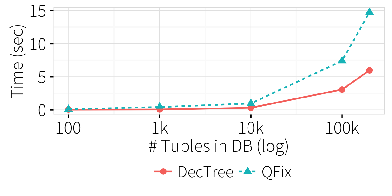
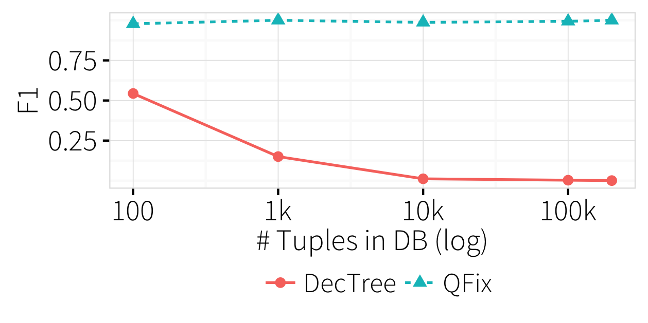
Figure 10(a) shows that although the runtime performance of DecTree is better than QFix by small a constant factor (), both runtimes degrade exponentially. In addition, the DecTree repairs are effectively unusable as their accuracy is low: the F1-score starts at and rapidly degrades towards . From these empirical results, we find that DecTree generates low-quality repairs even under the simplest conditions—an approach that applies DecTree over more queries is expected to have little hope of succeeding.
There are three important reasons why DecTree, and any approach that focuses on a single query at a time222Although our incremental approach tries to generate a repair for a single query at a time, it encodes all subsequent queries in the log., will not perform well.
-
•
Single Query Limitation: In principle, one could attempt to apply this technique to the entire log one query at a time, starting from the most recent query. Even ignoring the low repair accuracy shown in Figure 10(b), this approach is infeasible. Consider that we generate a labeled training dataset to repair using the query’s input and output database states and . Note that is the theoretically correct database state assuming no errors in the query log. We would need to derive by applying the complaint set to to create , and roll back the database state. Unfortunately, UPDATE queries are commonly surjective such that their inverses are ambiguous, which means that it is often impossible to derive . In contrast, the incremental version of QFix can bypass this problem by encoding subsequent queries in the log in a MILP representation.
-
•
Structurally Different WHERE Clause Results: The basic classifier approach simply learns a set of rules to minimize classification error, and can derive a clause whose struture is arbitrarily different from the original query’s WHERE clause. Although it may be possible to incorporate a distance measure as part of the decision tree splitting criteria, it is likely to be a heuristic with no guarantees.
-
•
High Selectivity, Low Precision: Classifiers try to avoid overfitting by balancing the complexity of the rules with classification accuracy. This is problematic for highly selective queries (e.g., primary key updates), because the classifier may simply ignore the single incorrect record and generate a rule such as FALSE. In fact, this form of severely imbalanced data continues to be a challenge for most major classification algorithms [26, 20]. Thus, we believe that alternative classification algorithms would not improve on these results. Compound with the fact that many workloads are primarily composed of key update queries [16] this issue severely limits the applicability of learning-based approaches.