Entanglement negativity in free-fermion systems: An overlap matrix approach

Po-Yao Chang Center for Materials Theory, Rutgers University, Piscataway, New Jersey, 08854, USA Department of Physics, University of Illinois at Urbana-Champaign, Urbana, Illinois, 61801, USA    Xueda Wen Department of Physics, University of Illinois at Urbana-Champaign, Urbana, Illinois, 61801, USA
Abstract

In this paper, we calculate the entanglement negativity in free-fermion systems by use of the overlap matrices. For a tripartite system, if the ground state can be factored into triples of modes, we show that the partially transposed reduced density matrix can be factorized and the entanglement negativity has a simple form. However, the factorability of the ground state in a tripartite system does not hold in general. In this situation, the partially transposed reduced density matrix can be expressed in terms of the Kronecker product of matrices. We explicitly compute the entanglement negativity for the Su-Schrieffer-Heeger model, the integer Quantum Hall state, and a homogeneous one-dimensional chain. We find that the entanglement negativity for the integer quantum Hall states shows an area law behavior. For the entanglement negativity of two adjacent intervals in a homogeneous one-dimensional gas, we find agreement with the conformal field theory. Our method provides a numerically feasible way to study the entanglement negativity in free-fermion systems.

I Introduction

The study of quantum entanglement provides a powerful tool to analyze the many-body states in condensed matter physicsKitaev ; Levin ; Calabrese0 ; Amico ; Eisert ; Vidal0 ; Calabrese00 ; Calabrese000 ; Benatti ; Benatti2 . The most celebrated measure of entanglement is given by the entanglement entropy (von Neumann entropy) SAsubscript𝑆𝐴S_{A} of the reduced density matrix of the subsystem A𝐴A. This quantity measures the entanglement between two complementary subsystems A𝐴A and B𝐡B, when the total system is in a pure state. One remarkably common result is an area law behavior of the entanglement entropy in gapped systems, which grows proportionally with the boundary between two subsystemsEisert . An important exception is the one-dimensional systems at criticality, where the entanglement entropy has a logarithmic scaling behaviorCalabrese0 ; Vidal0 ; Eisert and have been understood by use of a conformal field theory (CFT) approachCalabrese000 ; Calabrese0 .

However, using the entanglement entropy as a probe to diagonalize the entanglement for a mixed state is a difficult task. It requires a heavy optimization process. Hence, an alternative measure of entanglement for a mixed state has been proposedβ€”the entanglement negativityEisert1 ; Vidal ; Plenio . The advantage of using entanglement negativity is that it only requires linear algebraic computations. The entanglement negativity is defined as follows. Suppose a tripartite system is divided into A1subscript𝐴1A_{1}, A2subscript𝐴2A_{2}, and B𝐡B subsystems. The ground state after tracing out the degrees of freedom in a B𝐡B subsystem is a general mixed state. The entanglement negativity, which quantifies the entanglement between A1subscript𝐴1A_{1} and A2subscript𝐴2A_{2}, is obtained by partially transposing (with respect to the degrees of freedom in A2subscript𝐴2A_{2}) the reduced density matrix ρA1βˆͺA2subscript𝜌subscript𝐴1subscript𝐴2\rho_{A_{1}\cup A_{2}}, which is denoted as ρA1βˆͺA2TA2superscriptsubscript𝜌subscript𝐴1subscript𝐴2subscript𝑇subscript𝐴2\rho_{A_{1}\cup A_{2}}^{T_{A_{2}}}. Then the entanglement negativity between subsystems A1subscript𝐴1A_{1} and A2subscript𝐴2A_{2} is defined as

β„°:=ln⁑Tr​|ρA1βˆͺA2TA2|,assignβ„°Trsuperscriptsubscript𝜌subscript𝐴1subscript𝐴2subscript𝑇subscript𝐴2\displaystyle\mathcal{E}:=\ln\mathrm{Tr}|\rho_{A_{1}\cup A_{2}}^{T_{A_{2}}}|, (1)

where the trace norm |ρA1βˆͺA2TA2|superscriptsubscript𝜌subscript𝐴1subscript𝐴2subscript𝑇subscript𝐴2|\rho_{A_{1}\cup A_{2}}^{T_{A_{2}}}| represents the sum of all absolute values of the eigenvalues of ρA1βˆͺA2TA2superscriptsubscript𝜌subscript𝐴1subscript𝐴2subscript𝑇subscript𝐴2\rho_{A_{1}\cup A_{2}}^{T_{A_{2}}}. Recently, the entanglement negativity has been extensively studied in numerous many-body systems, e.g., harmonic oscillators in one dimensionAudenaert ; Marcovitch ; Ferraro ; Cavalcanti ; Anders ; Anders1 , quantum spin chainsWichterich2 ; Wichterich3 ; Bayat ; Bayat2 ; Bayat3 ; Santos , systems with topological orders Castelnovo ; Lee , and (2+1) dimensional Chern-Simons theoriesEN_CS . A CFT approachCalabrese ; Calabrese2 and many useful numerical methods are also developed, including tree tensor techniquesCalabrese5 , Monte Carlo simulationsAlba ; Chung , and rational interpolationsNobili . Further studies on non-equilibrium situationsEisler ; Coser ; Hoogeveen ; Wen and finite temperatureCalabrese4 ; Eisler refine our understanding of the entanglement negativity.

In this work, we demonstrate a systematical way to compute the entanglement negativity in free-fermion systems by using the overlap matrices. For the prior works on entanglement negativity in free fermion systemsEisler2 ; Coser2 ; Coser3 ; Eisler3 ; Coser4 , the quantities people calculated are the moments of partially transposed reduced denity matrix (ρA1βˆͺA2TA2)nsuperscriptsuperscriptsubscript𝜌subscript𝐴1subscript𝐴2subscript𝑇subscript𝐴2𝑛\left(\rho_{A_{1}\cup A_{2}}^{T_{A_{2}}}\right)^{n}, with nβ‰₯2𝑛2n\geq 2. In other words, the entanglement negativity, which is obtained from the trace norm |ρA1βˆͺA2TA2|superscriptsubscript𝜌subscript𝐴1subscript𝐴2subscript𝑇subscript𝐴2\left|\rho_{A_{1}\cup A_{2}}^{T_{A_{2}}}\right|, has not been computed in the prior works due to reasons of technical difficulty. In our work, we will give an explicit calculation of |ρA1βˆͺA2TA2|superscriptsubscript𝜌subscript𝐴1subscript𝐴2subscript𝑇subscript𝐴2\left|\rho_{A_{1}\cup A_{2}}^{T_{A_{2}}}\right| by using the overlap matrices, and therefore the entanglement negativity is obtained. The overlap matrices are built up from the single-particle states Ο•nsubscriptitalic-ϕ𝑛\phi_{n} corresponding to the lowest N𝑁N (occupied) energy levels of the systemIsrael ; Calabrese6 ; Calabrese3 ; Calabrese7 ; Ossipov ; Drut :

[MΟƒ]n​m=βˆ«ΟƒddxΟ•nβˆ—(x)Ο•m(x),,n,m=1,β‹―,N,\displaystyle[M_{\sigma}]_{nm}=\int_{\sigma}d^{d}x\phi_{n}^{*}(x)\phi_{m}(x),\quad,n,m=1,\cdots,N, (2)

where the integration is restricted to the subsystems Οƒ=A1,A2𝜎subscript𝐴1subscript𝐴2\sigma=A_{1},A_{2} or B𝐡B in arbitrary dimension d𝑑d. We show that for a tripartite system, when the overlap matrices MA1subscript𝑀subscript𝐴1M_{A_{1}}, MA2subscript𝑀subscript𝐴2M_{A_{2}}, and MBsubscript𝑀𝐡M_{B} can be simultaneously diagonalized, the ground state of fermions can be factored into triples of modes. In this situation, the partially transposed reduced density matrix can be factorized and the entanglement negativity can be obtained from the spectra of the overlap matrices. On the other hand, when the simultaneous diagonalizability of the overlap matrices does not hold, the factorability of the ground state in a tripartite system is failed. In this situation, the partially transposed reduced density matrix can only be expressed in terms of the Kronecker product of matrices. Then the entanglement negativity is directly obtained from the partially transposed reduced density matrix. The overlap matrix approach provides a systematical way to calculate the entanglement negativity in any free-fermion systems, which can be either gapped topological phases or critical systems. This approach is also applicable for disordered systems and can be extended to higher dimensions.

The paper is organized as follows: In Sec. II, we review the entanglement negativity for a pure state. In Sec. III.1, we obtain the entanglement negativity for a mixed state when the ground state can be factored into triples of modes in a tripartite system. We find that the entanglement negativity for the integer quantum Hall state satisfies an area law. In Sec. III.2, we derive the entanglement negativity for a general mixed state. We compute the entanglement negativity for free fermions on a ring and show the entanglement negativity is in agreement with CFT. In Sec. IV, we conclude our results.

II Entanglement negativity in free-fermion systems for pure states

Let us start with the Hamiltonian for free fermions

H=βˆ‘Ξ±=1Mϡα​dα†​dΞ±,withΟ΅1β©½Ο΅2β©½β‹―β©½Ο΅M,formulae-sequence𝐻superscriptsubscript𝛼1𝑀subscriptitalic-ϡ𝛼subscriptsuperscript𝑑†𝛼subscript𝑑𝛼withsubscriptitalic-Ο΅1subscriptitalic-Ο΅2β‹―subscriptitalic-Ο΅M\displaystyle H=\sum_{\alpha=1}^{M}\epsilon_{\alpha}d^{\dagger}_{\alpha}d_{\alpha},\rm{with}\quad\epsilon_{1}\leqslant\epsilon_{2}\leqslant\cdots\leqslant\epsilon_{M}, (3)

where dΞ±subscript𝑑𝛼d_{\alpha} is the fermion operator with corresponding energy ϡαsubscriptitalic-ϡ𝛼\epsilon_{\alpha}, and M𝑀M is the number of bands. The ground state is

|Ψ⟩=∏α=1Ndα†​|0⟩,ketΞ¨superscriptsubscriptproduct𝛼1𝑁subscriptsuperscript𝑑†𝛼ket0\displaystyle|\Psi\rangle=\prod_{\alpha=1}^{N}d^{\dagger}_{\alpha}|0\rangle, (4)

where N𝑁N is the total number of particles in the system. We consider a bipartite system that the system is partitioned into A𝐴A and B𝐡B parts and the single-particle wave function can be partitioned by the projection operator 𝒫A​(B)subscript𝒫𝐴𝐡\mathcal{P}_{A(B)}. Following Ref. [Israel, ], we introduce an overlap matrix,

[MA​(B)]α​βsubscriptdelimited-[]subscript𝑀𝐴𝐡𝛼𝛽\displaystyle[M_{A(B)}]_{\alpha\beta} =βŸ¨π’«A​(B)​uΞ±,𝒫A​(B)​uβ⟩absentsubscript𝒫𝐴𝐡subscript𝑒𝛼subscript𝒫𝐴𝐡subscript𝑒𝛽\displaystyle=\langle\mathcal{P}_{A(B)}u_{\alpha},\mathcal{P}_{A(B)}u_{\beta}\rangle
=∫r∈A​(B)dd​rβ€‹Ο•Ξ±βˆ—β€‹(𝐫)​ϕβ​(𝐫),with1β©½Ξ±,Ξ²β©½N,formulae-sequenceabsentsubscriptπ‘Ÿπ΄π΅superscriptπ‘‘π‘‘π‘Ÿsubscriptsuperscriptitalic-ϕ𝛼𝐫subscriptitalic-ϕ𝛽𝐫withformulae-sequence1𝛼𝛽N\displaystyle=\int_{r\in A(B)}d^{d}r\phi^{*}_{\alpha}({\bf r})\phi_{\beta}({\bf r}),\rm{with}\quad 1\leqslant\alpha,\beta\leqslant N, (5)

where |uα⟩=dα†​|0⟩ketsubscript𝑒𝛼subscriptsuperscript𝑑†𝛼ket0|u_{\alpha}\rangle=d^{\dagger}_{\alpha}|0\rangle and 𝒫A​(B)subscript𝒫𝐴𝐡\mathcal{P}_{A(B)} is the orthogonal projection operator on Hilbert space A​(B)𝐴𝐡A(B), such that 𝒫A​(B)​|uα⟩=ϕα​(𝐫)|π«βˆˆπ€β€‹(𝐁)subscript𝒫𝐴𝐡ketsubscript𝑒𝛼evaluated-atsubscriptitalic-ϕ𝛼𝐫𝐫𝐀𝐁\mathcal{P}_{A(B)}|u_{\alpha}\rangle=\phi_{\alpha}({\bf r})|_{\bf r\in A(B)}. Since MB=π•€βˆ’MAsubscript𝑀𝐡𝕀subscript𝑀𝐴M_{B}=\mathbb{I}-M_{A}, one can find a unitary matrix Ui​αsubscriptπ‘ˆπ‘–π›ΌU_{i\alpha} that simultaneously diagonalizes MAsubscript𝑀𝐴M_{A} and MBsubscript𝑀𝐡M_{B}, such that U​MA​U†=diag​(Pi)π‘ˆsubscript𝑀𝐴superscriptπ‘ˆβ€ diagsubscript𝑃𝑖UM_{A}U^{\dagger}={\rm diag}(P_{i}) and U​MB​U†=diag​(1βˆ’Pi)π‘ˆsubscript𝑀𝐡superscriptπ‘ˆβ€ diag1subscript𝑃𝑖UM_{B}U^{\dagger}={\rm diag}(1-P_{i}). The single-particle Hilbert space is decomposed into two parts β„‹=β„‹A​⨁ℋBβ„‹subscriptℋ𝐴direct-sumsubscriptℋ𝐡\mathcal{H}=\mathcal{H}_{A}\bigoplus\mathcal{H}_{B}. The orthonormal modes at β„‹Asubscriptℋ𝐴\mathcal{H}_{A} and β„‹Bsubscriptℋ𝐡\mathcal{H}_{B} are

|Ai⟩=βˆ‘Ξ±Ui​α†​𝒫A​|uα⟩Pi,|Bi⟩=βˆ‘Ξ±Ui​α†​𝒫B​|uα⟩1βˆ’Pi.formulae-sequenceketsubscript𝐴𝑖subscript𝛼subscriptsuperscriptπ‘ˆβ€ π‘–π›Όsubscript𝒫𝐴ketsubscript𝑒𝛼subscript𝑃𝑖ketsubscript𝐡𝑖subscript𝛼subscriptsuperscriptπ‘ˆβ€ π‘–π›Όsubscript𝒫𝐡ketsubscript𝑒𝛼1subscript𝑃𝑖\displaystyle|A_{i}\rangle=\frac{\sum_{\alpha}U^{\dagger}_{i\alpha}\mathcal{P}_{A}|u_{\alpha}\rangle}{\sqrt{P_{i}}},\quad|B_{i}\rangle=\frac{\sum_{\alpha}U^{\dagger}_{i\alpha}\mathcal{P}_{B}|u_{\alpha}\rangle}{\sqrt{1-P_{i}}}. (6)

Let E=span​(|uα⟩;1β©½Ξ±β©½N)𝐸spanketsubscriptu𝛼1𝛼NE=\rm{span}(|u_{\alpha}\rangle;1\leqslant\alpha\leqslant N) is the subspace of the single particle Hilbert space β„‹β„‹\mathcal{H}. Since Uπ‘ˆU is unitary, we have E=span​(Ui​α†​|uα⟩)𝐸spansubscriptsuperscriptπ‘ˆβ€ π‘–π›Όketsubscript𝑒𝛼E={\rm span}(U^{\dagger}_{i\alpha}|u_{\alpha}\rangle). The ground state in Eq. (4) can be rotated by this unitary matrix Uπ‘ˆU. By using

βˆ‘Ξ±Ui​α†​dα†​|0⟩subscript𝛼subscriptsuperscriptπ‘ˆβ€ π‘–π›Όsubscriptsuperscript𝑑†𝛼ket0\displaystyle\sum_{\alpha}U^{\dagger}_{i\alpha}d^{\dagger}_{\alpha}|0\rangle =βˆ‘Ξ±Ui​α†​|uα⟩=βˆ‘Ξ±Ui​α†​(𝒫A​|uα⟩+𝒫B​|uα⟩)absentsubscript𝛼subscriptsuperscriptπ‘ˆβ€ π‘–π›Όketsubscript𝑒𝛼subscript𝛼subscriptsuperscriptπ‘ˆβ€ π‘–π›Όsubscript𝒫𝐴ketsubscript𝑒𝛼subscript𝒫𝐡ketsubscript𝑒𝛼\displaystyle=\sum_{\alpha}U^{\dagger}_{i\alpha}|u_{\alpha}\rangle=\sum_{\alpha}U^{\dagger}_{i\alpha}(\mathcal{P}_{A}|u_{\alpha}\rangle+\mathcal{P}_{B}|u_{\alpha}\rangle)
=Pi​|Ai⟩+1βˆ’Pi​|Bi⟩,absentsubscript𝑃𝑖ketsubscript𝐴𝑖1subscript𝑃𝑖ketsubscript𝐡𝑖\displaystyle=\sqrt{P_{i}}|A_{i}\rangle+\sqrt{1-P_{i}}|B_{i}\rangle, (7)

the ground state under the rotation can be written as (up to a global phase)

|Ψ⟩=∏i=1N(Pi​dA​i†+1βˆ’Pi​dBi†)​|0⟩,ketΞ¨superscriptsubscriptproduct𝑖1𝑁subscript𝑃𝑖subscriptsuperscript𝑑†𝐴𝑖1subscript𝑃𝑖subscriptsuperscript𝑑†subscript𝐡𝑖ket0\displaystyle|\Psi\rangle=\prod_{i=1}^{N}(\sqrt{P_{i}}d^{\dagger}_{Ai}+\sqrt{1-P_{i}}d^{\dagger}_{B_{i}})|0\rangle, (8)

where dA​(B)​i†​|0⟩=|A​(B)i⟩subscriptsuperscript𝑑†𝐴𝐡𝑖ket0ket𝐴subscript𝐡𝑖d^{\dagger}_{A(B)i}|0\rangle=|A(B)_{i}\rangle.

We can compute the entanglement negativity directly from the partially transposed density matrix ρTBsuperscript𝜌subscript𝑇𝐡\rho^{T_{B}}. The density matrix from the ground state under occupation basis in Eq. (4) is

ρ=⨂i(PiPi​(1βˆ’Pi)Pi​(1βˆ’Pi)1βˆ’Pi),𝜌subscripttensor-product𝑖subscript𝑃𝑖subscript𝑃𝑖1subscript𝑃𝑖subscript𝑃𝑖1subscript𝑃𝑖1subscript𝑃𝑖\displaystyle\rho=\bigotimes_{i}\left(\begin{array}[]{cc}P_{i}&\sqrt{P_{i}(1-P_{i})}\\ \sqrt{P_{i}(1-P_{i})}&1-P_{i}\end{array}\right), (11)

where the basis is {|1A​i​0B​i⟩,|0A​i​1B​i⟩}ketsubscript1𝐴𝑖subscript0𝐡𝑖ketsubscript0𝐴𝑖subscript1𝐡𝑖\{|1_{Ai}0_{Bi}\rangle,|0_{Ai}1_{Bi}\rangle\}.

The partially transposed density matrix ρTBsuperscript𝜌subscript𝑇𝐡\rho^{T_{B}} is

ρTBsuperscript𝜌subscript𝑇𝐡\displaystyle\rho^{T_{B}} =⨂iρiTBabsentsubscripttensor-product𝑖superscriptsubscriptπœŒπ‘–subscript𝑇𝐡\displaystyle=\bigotimes_{i}\rho_{i}^{T_{B}}
=⨂i(Pi00001βˆ’Pi00000Pi​(1βˆ’Pi)00Pi​(1βˆ’Pi)0),absentsubscripttensor-product𝑖subscript𝑃𝑖00001subscript𝑃𝑖00000subscript𝑃𝑖1subscript𝑃𝑖00subscript𝑃𝑖1subscript𝑃𝑖0\displaystyle=\bigotimes_{i}\left(\begin{array}[]{cccc}P_{i}&0&0&0\\ 0&1-P_{i}&0&0\\ 0&0&0&\sqrt{P_{i}(1-P_{i})}\\ 0&0&\sqrt{P_{i}(1-P_{i})}&0\end{array}\right), (16)

where the basis is {|1A​i​0B​i⟩,|0A​i​1B​i⟩,|0A​i​0B​i⟩,|1A​i​1B​i⟩}ketsubscript1𝐴𝑖subscript0𝐡𝑖ketsubscript0𝐴𝑖subscript1𝐡𝑖ketsubscript0𝐴𝑖subscript0𝐡𝑖ketsubscript1𝐴𝑖subscript1𝐡𝑖\{|1_{Ai}0_{Bi}\rangle,|0_{Ai}1_{Bi}\rangle,|0_{Ai}0_{Bi}\rangle,|1_{Ai}1_{Bi}\rangle\}.

Notice that the eigenvalues of the Kronecker product of two matrices WAβŠ—WBtensor-productsubscriptπ‘Šπ΄subscriptπ‘Šπ΅W_{A}\otimes W_{B} are Ξ»i​μjsubscriptπœ†π‘–subscriptπœ‡π‘—\lambda_{i}\mu_{j}, where Ξ»isubscriptπœ†π‘–\lambda_{i} and ΞΌjsubscriptπœ‡π‘—\mu_{j} are the eigenvalues of WAsubscriptπ‘Šπ΄W_{A} and WBsubscriptπ‘Šπ΅W_{B}, respectively. The eigenvalues of ρTBsuperscript𝜌subscript𝑇𝐡\rho^{T_{B}} are the product of one of the eigenvalues of each ρiTBsuperscriptsubscriptπœŒπ‘–subscript𝑇𝐡\rho_{i}^{T_{B}}. The set of eigenvalues of ρiTBsuperscriptsubscriptπœŒπ‘–subscript𝑇𝐡\rho_{i}^{T_{B}} is {Ξi,Ξ±}={Pi,1βˆ’Pi,Pi​(1βˆ’Pi),βˆ’Pi​(1βˆ’Pi)}subscriptΞžπ‘–π›Όsubscript𝑃𝑖1subscript𝑃𝑖subscript𝑃𝑖1subscript𝑃𝑖subscript𝑃𝑖1subscript𝑃𝑖\{\Xi_{i,\alpha}\}=\{P_{i},1-P_{i},\sqrt{P_{i}(1-P_{i})},-\sqrt{P_{i}(1-P_{i})}\} with α𝛼\alpha being the label of the elements in the set. Hence the entanglement is

β„°β„°\displaystyle\mathcal{E} =lnTr​|ρTB|=lnβ€‹βˆiβˆ‘Ξ±(|Ξi,Ξ±|)absentlnTrsuperscript𝜌subscript𝑇𝐡lnsubscriptproduct𝑖subscript𝛼subscriptΞžπ‘–π›Ό\displaystyle=\mathrm{lnTr}|\rho^{T_{B}}|=\mathrm{ln}\prod_{i}\sum_{\alpha}(|\Xi_{i,\alpha}|)
=βˆ‘iln​(1+2​Pi​(1βˆ’Pi)).absentsubscript𝑖ln12subscript𝑃𝑖1subscript𝑃𝑖\displaystyle=\sum_{i}\mathrm{ln}(1+2\sqrt{P_{i}(1-P_{i})}). (17)

Examples of the entanglement negativity for pure states are shown in App. A.

III Entanglement negativity in free-fermion systems for mixed states

III.1 The ground state in a tripartite system can be factored into triples of modes

Now we generalize the bipartite case to a tripartite system. The overlap matrices MA1subscript𝑀subscript𝐴1M_{A_{1}}, MA2subscript𝑀subscript𝐴2M_{A_{2}}, and MBsubscript𝑀𝐡M_{B} are constructed from Eq. (5), with the projected single-particle wave function 𝒫A1​|uα⟩subscript𝒫subscript𝐴1ketsubscript𝑒𝛼\mathcal{P}_{A_{1}}|u_{\alpha}\rangle, 𝒫A2​|uα⟩subscript𝒫subscript𝐴2ketsubscript𝑒𝛼\mathcal{P}_{A_{2}}|u_{\alpha}\rangle, and 𝒫B​|uα⟩subscript𝒫𝐡ketsubscript𝑒𝛼\mathcal{P}_{B}|u_{\alpha}\rangle. If the overlap matrices can be simultaneously diagonalized by a unitary matrix Ui​αsubscriptπ‘ˆπ‘–π›ΌU_{i\alpha}, we can find the orthonormal modes at the subsystems

|A1​i⟩=βˆ‘Ξ±Ui​α†​𝒫A1​|uα⟩P1​i,|A2​i⟩=βˆ‘Ξ±Ui​α†​𝒫A2​|uα⟩P2​i,formulae-sequenceketsubscript𝐴1𝑖subscript𝛼subscriptsuperscriptπ‘ˆβ€ π‘–π›Όsubscript𝒫subscript𝐴1ketsubscript𝑒𝛼subscript𝑃1𝑖ketsubscript𝐴2𝑖subscript𝛼subscriptsuperscriptπ‘ˆβ€ π‘–π›Όsubscript𝒫subscript𝐴2ketsubscript𝑒𝛼subscript𝑃2𝑖\displaystyle|A_{1i}\rangle=\frac{\sum_{\alpha}U^{\dagger}_{i\alpha}\mathcal{P}_{A_{1}}|u_{\alpha}\rangle}{\sqrt{P_{1i}}},\quad|A_{2i}\rangle=\frac{\sum_{\alpha}U^{\dagger}_{i\alpha}\mathcal{P}_{A_{2}}|u_{\alpha}\rangle}{\sqrt{P_{2i}}}, (18)
|Bi⟩=βˆ‘Ξ±Ui​α†​𝒫B​|uα⟩1βˆ’P1​iβˆ’P2​i.ketsubscript𝐡𝑖subscript𝛼subscriptsuperscriptπ‘ˆβ€ π‘–π›Όsubscript𝒫𝐡ketsubscript𝑒𝛼1subscript𝑃1𝑖subscript𝑃2𝑖\displaystyle|B_{i}\rangle=\frac{\sum_{\alpha}U^{\dagger}_{i\alpha}\mathcal{P}_{B}|u_{\alpha}\rangle}{\sqrt{1-P_{1i}-P_{2i}}}.

Since the single-particle Hilbert space does note change under unitary transformation, i.e., E=span​(|uα⟩)=span​(Ui​α†​|uα⟩)𝐸spanketsubscript𝑒𝛼spansubscriptsuperscriptπ‘ˆβ€ π‘–π›Όketsubscript𝑒𝛼E={\rm span}(|u_{\alpha}\rangle)={\rm span}(U^{\dagger}_{i\alpha}|u_{\alpha}\rangle), and

βˆ‘Ξ±Ui​α†​dα†​|0⟩=βˆ‘Ξ±Ui​α†​|uα⟩subscript𝛼superscriptsubscriptπ‘ˆπ‘–π›Όβ€ subscriptsuperscript𝑑†𝛼ket0subscript𝛼superscriptsubscriptπ‘ˆπ‘–π›Όβ€ ketsubscript𝑒𝛼\displaystyle\sum_{\alpha}U_{i\alpha}^{\dagger}d^{\dagger}_{\alpha}|0\rangle=\sum_{\alpha}U_{i\alpha}^{\dagger}|u_{\alpha}\rangle
=βˆ‘Ξ±Ui​α†​(𝒫A1​|uα⟩+𝒫A2​|uα⟩+𝒫B​|uα⟩)absentsubscript𝛼subscriptsuperscriptπ‘ˆβ€ π‘–π›Όsubscript𝒫subscript𝐴1ketsubscript𝑒𝛼subscript𝒫subscript𝐴2ketsubscript𝑒𝛼subscript𝒫𝐡ketsubscript𝑒𝛼\displaystyle=\sum_{\alpha}U^{\dagger}_{i\alpha}(\mathcal{P}_{A_{1}}|u_{\alpha}\rangle+\mathcal{P}_{A_{2}}|u_{\alpha}\rangle+\mathcal{P}_{B}|u_{\alpha}\rangle)
=(P1​i​|A1​i⟩+P2​i​|A2​i⟩+1βˆ’P1​iβˆ’P2​i​|Bi⟩),absentsubscript𝑃1𝑖ketsubscript𝐴1𝑖subscript𝑃2𝑖ketsubscript𝐴2𝑖1subscript𝑃1𝑖subscript𝑃2𝑖ketsubscript𝐡𝑖\displaystyle=(\sqrt{P_{1i}}|A_{1i}\rangle+\sqrt{P_{2i}}|A_{2i}\rangle+\sqrt{1-P_{1i}-P_{2i}}|B_{i}\rangle), (19)

the ground state can be factored into triples of modes

|Ψ⟩ketΞ¨\displaystyle|\Psi\rangle =∏i(P1​i​dA1​i†+P2​i​dA2​i†+1βˆ’P1​iβˆ’P2​i​dB​i†)​|0⟩.absentsubscriptproduct𝑖subscript𝑃1𝑖subscriptsuperscript𝑑†subscript𝐴1𝑖subscript𝑃2𝑖subscriptsuperscript𝑑†subscript𝐴2𝑖1subscript𝑃1𝑖subscript𝑃2𝑖subscriptsuperscript𝑑†𝐡𝑖ket0\displaystyle=\prod_{i}(\sqrt{P_{1i}}d^{\dagger}_{A_{1}i}+\sqrt{P_{2i}}d^{\dagger}_{A_{2}i}+\sqrt{1-P_{1i}-P_{2i}}d^{\dagger}_{Bi})|0\rangle. (20)

where dσ​i†​|0⟩=|Οƒi⟩subscriptsuperscriptπ‘‘β€ πœŽπ‘–ket0ketsubscriptπœŽπ‘–d^{\dagger}_{\sigma i}|0\rangle=|\sigma_{i}\rangle with Οƒ=A1,A2,B𝜎subscript𝐴1subscript𝐴2𝐡\sigma=A_{1},A_{2},B.

The reduced density matrix after tracing part B𝐡B is

ρA=⨂i(P1​iP1​i​P2​i00P1​i​P2​iP2​i00001βˆ’P1​iβˆ’P2​i00000),subscript𝜌𝐴subscripttensor-product𝑖subscript𝑃1𝑖subscript𝑃1𝑖subscript𝑃2𝑖00subscript𝑃1𝑖subscript𝑃2𝑖subscript𝑃2𝑖00001subscript𝑃1𝑖subscript𝑃2𝑖00000\displaystyle\rho_{A}=\bigotimes_{i}\left(\begin{array}[]{cccc}P_{1i}&\sqrt{P_{1i}P_{2i}}&0&0\\ \sqrt{P_{1i}P_{2i}}&P_{2i}&0&0\\ 0&0&1-P_{1i}-P_{2i}&0\\ 0&0&0&0\end{array}\right), (25)

where the basis of the reduced density is {|1A1​0A2⟩i,|0A1​1A2⟩i,|0A1​0A2⟩i,|1A1​1A2⟩i}subscriptketsubscript1subscript𝐴1subscript0subscript𝐴2𝑖subscriptketsubscript0subscript𝐴1subscript1subscript𝐴2𝑖subscriptketsubscript0subscript𝐴1subscript0subscript𝐴2𝑖subscriptketsubscript1subscript𝐴1subscript1subscript𝐴2𝑖\{|1_{A_{1}}0_{A_{2}}\rangle_{i},|0_{A_{1}}1_{A_{2}}\rangle_{i},|0_{A_{1}}0_{A_{2}}\rangle_{i},|1_{A_{1}}1_{A_{2}}\rangle_{i}\}.

The partially transposed reduced density matrix after transposing the A2subscript𝐴2A_{2} is

ρATA2superscriptsubscript𝜌𝐴subscript𝑇subscript𝐴2\displaystyle\rho_{A}^{T_{A_{2}}} =⨂iρA​iTA2absentsubscripttensor-product𝑖superscriptsubscriptπœŒπ΄π‘–subscript𝑇subscript𝐴2\displaystyle=\bigotimes_{i}\rho_{Ai}^{T_{A_{2}}}
=⨂i(P1​i0000P2​i00001βˆ’P1​iβˆ’P2​iP1​i​P2​i00P1​i​P2​i0).absentsubscripttensor-product𝑖subscript𝑃1𝑖0000subscript𝑃2𝑖00001subscript𝑃1𝑖subscript𝑃2𝑖subscript𝑃1𝑖subscript𝑃2𝑖00subscript𝑃1𝑖subscript𝑃2𝑖0\displaystyle=\bigotimes_{i}\left(\begin{array}[]{cccc}P_{1i}&0&0&0\\ 0&P_{2i}&0&0\\ 0&0&1-P_{1i}-P_{2i}&\sqrt{P_{1i}P_{2i}}\\ 0&0&\sqrt{P_{1i}P_{2i}}&0\end{array}\right). (30)

The set of eigenvalues of ρA​iTA2superscriptsubscriptπœŒπ΄π‘–subscript𝑇subscript𝐴2\rho_{Ai}^{T_{A_{2}}} is {Ξi,Ξ±}={P1​i,P2​i,12​(1βˆ’P1​iβˆ’P2​iΒ±(1βˆ’P1​iβˆ’P2​i)2+4​P1​i​P2​i)}subscriptΞžπ‘–π›Όsubscript𝑃1𝑖subscript𝑃2𝑖12plus-or-minus1subscript𝑃1𝑖subscript𝑃2𝑖superscript1subscript𝑃1𝑖subscript𝑃2𝑖24subscript𝑃1𝑖subscript𝑃2𝑖\{\Xi_{i,\alpha}\}=\{P_{1i},P_{2i},\frac{1}{2}(1-P_{1i}-P_{2i}\pm\sqrt{(1-P_{1i}-P_{2i})^{2}+4P_{1i}P_{2i}})\} with α𝛼\alpha being the label of the elements in the set. The entanglement negativity is

β„°β„°\displaystyle\mathcal{E} =lnTr​|ρATA2|=βˆ‘iln​(βˆ‘Ξ±|Ξi,Ξ±|)absentlnTrsuperscriptsubscript𝜌𝐴subscript𝑇subscript𝐴2subscript𝑖lnsubscript𝛼subscriptΞžπ‘–π›Ό\displaystyle=\mathrm{lnTr}|\rho_{A}^{T_{A_{2}}}|=\sum_{i}\mathrm{ln}(\sum_{\alpha}|\Xi_{i,\alpha}|)
=βˆ‘iln⁑(P1​i+P2​i+(1βˆ’P1​iβˆ’P2​i)2+4​P1​i​P2​i).absentsubscript𝑖subscript𝑃1𝑖subscript𝑃2𝑖superscript1subscript𝑃1𝑖subscript𝑃2𝑖24subscript𝑃1𝑖subscript𝑃2𝑖\displaystyle=\sum_{i}\ln(P_{1i}+P_{2i}+\sqrt{(1-P_{1i}-P_{2i})^{2}+4P_{1i}P_{2i}}). (31)

Notice that if the probability for all the eigenstates in subsystem B𝐡B is zero, which can be realized by taking the dimension of Hilbert space of B𝐡B to be zero, the entanglement negativity becomes the case of pure states,

limdim.ℬ→0β„°subscriptformulae-sequencedim→ℬ0β„°\displaystyle\lim_{\mathrm{dim.}\mathcal{B}\to 0}\mathcal{E} =βˆ‘iln⁑(1+2​P1​i​P2​i)absentsubscript𝑖12subscript𝑃1𝑖subscript𝑃2𝑖\displaystyle=\sum_{i}\ln(1+2\sqrt{P_{1i}P_{2i}})
=βˆ‘iln⁑(1+2​P1​i​(1βˆ’P1​i)),absentsubscript𝑖12subscript𝑃1𝑖1subscript𝑃1𝑖\displaystyle=\sum_{i}\ln(1+2\sqrt{P_{1i}(1-P_{1i})}), (32)

where ℬℬ\mathcal{B} is the Hibert space of region B𝐡B.

In the following, we consider the entanglement negativity between A1subscript𝐴1A_{1} and A2subscript𝐴2A_{2} regions of two examples in which the overlap matrices can be simultaneously diagonalized. The first one is the fully dimerized Su-Schrieffer-Heeger (SSH) model and the second one is the integer quantum Hall state (IQHS).

III.1.1 Dimerized Su-Schrieffer-Heeger (SSH) model

Refer to caption
Figure 1: The tripartite configuration of a dimerized Su-Schrieffer-Heeger model. The hopping amplitude of solid lines is t2subscript𝑑2t_{2}. One unit cell contains two orbitals that are pictured by βˆ™βˆ™\bullet and ∘\circ. The system is divided into A1subscript𝐴1A_{1}, A2subscript𝐴2A_{2} and B𝐡B parts by the red dashed lines. (a) Adjacent intervals for A1subscript𝐴1A_{1} and A2subscript𝐴2A_{2} regions. (b) Disjointed intervals for A1subscript𝐴1A_{1} and A2subscript𝐴2A_{2} regions.

The Su-Schrieffer-Heeger model is first introduced in Ref. [Su79, ], which describes one-dimensional polyacetylene. The Hamiltonian of a dimerized SSH model is

H=βˆ‘it​cai+1†​cbi+h.c.,formulae-sequence𝐻subscript𝑖𝑑subscriptsuperscript𝑐†subscriptπ‘Žπ‘–1subscript𝑐subscript𝑏𝑖hc\displaystyle H=\sum_{i}tc^{\dagger}_{a_{i+1}}c_{b_{i}}+\mathrm{h.c.}, (33)

where t𝑑t is the hopping amplitude and ca​(b)isubscriptπ‘π‘Žsubscript𝑏𝑖c_{a(b)_{i}} is the fermion operator. The ground state for this dimerized SSH model is

|Ψ⟩=∏αdα†​|0⟩,ketΞ¨subscriptproduct𝛼subscriptsuperscript𝑑†𝛼ket0\displaystyle|\Psi\rangle=\prod_{\alpha}d^{\dagger}_{\alpha}|0\rangle, (34)

where d1†=12​(ca,1β€ βˆ’cb,2†),d2†=12​(ca,2β€ βˆ’cb,3†),β‹―,dj†=12​(ca,jβ€ βˆ’cb,j+1†),β‹―formulae-sequencesuperscriptsubscript𝑑1†12subscriptsuperscriptπ‘β€ π‘Ž1subscriptsuperscript𝑐†𝑏2formulae-sequencesuperscriptsubscript𝑑2†12subscriptsuperscriptπ‘β€ π‘Ž2subscriptsuperscript𝑐†𝑏3β‹―superscriptsubscript𝑑𝑗†12subscriptsuperscriptπ‘β€ π‘Žπ‘—subscriptsuperscript𝑐†𝑏𝑗1β‹―d_{1}^{\dagger}=\frac{1}{\sqrt{2}}(c^{\dagger}_{a,1}-c^{\dagger}_{b,2}),d_{2}^{\dagger}=\frac{1}{\sqrt{2}}(c^{\dagger}_{a,2}-c^{\dagger}_{b,3}),\cdots,d_{j}^{\dagger}=\frac{1}{\sqrt{2}}(c^{\dagger}_{a,j}-c^{\dagger}_{b,j+1}),\cdots.

We consider an infinite chain that the system is divided into A1subscript𝐴1A_{1}, A2subscript𝐴2A_{2}, and B𝐡B as shown in Fig.Β 1. The state dj†​|0⟩=|uj⟩superscriptsubscript𝑑𝑗†ket0ketsubscript𝑒𝑗d_{j}^{\dagger}|0\rangle=|u_{j}\rangle is localized at aπ‘Ža orbital on j𝑗j-th site and at b𝑏b orbital on (j+1)𝑗1(j+1)-th site. This localized state is the eigenstate of three overlap matrices, MA1subscript𝑀subscript𝐴1M_{A_{1}}, MA2subscript𝑀subscript𝐴2M_{A_{2}}, and MBsubscript𝑀𝐡M_{B}. For the geometry shown in Fig. 1(a), the corresponding eigenvalues of MA1subscript𝑀subscript𝐴1M_{A_{1}} and MA2subscript𝑀subscript𝐴2M_{A_{2}} are,

P1​j=⟨uj|MA1|uj⟩={1,jβ©½iβˆ’2,0.5,j=iβˆ’1,0,jβ©Ύi.\displaystyle P_{1j}=\langle u_{j}|M_{A_{1}}|u_{j}\rangle=\left\{\begin{aligned} &1,\quad&j\leqslant i-2,\\ &0.5,\quad&j=i-1,\\ &0,\quad&j\geqslant i.\end{aligned}\right. (35)
P2​j=⟨uj|MA2|uj⟩={0.5,iβˆ’1β©½jβ©½i,0,otherwise.\displaystyle P_{2j}=\langle u_{j}|M_{A_{2}}|u_{j}\rangle=\left\{\begin{aligned} &0.5,\quad&i-1\leqslant j\leqslant i,\\ &0,\quad&{\rm otherwise}.\end{aligned}\right. (36)

For the geometry shown in Fig.1(b), the corresponding eigenvalues of MA1subscript𝑀subscript𝐴1M_{A_{1}} and MA2subscript𝑀subscript𝐴2M_{A_{2}} are,

P1​j=⟨uj|MA1|uj⟩={1,jβ©½iβˆ’2,0.5,j=iβˆ’1,0,jβ©Ύi.\displaystyle P_{1j}=\langle u_{j}|M_{A_{1}}|u_{j}\rangle=\left\{\begin{aligned} &1,\quad&j\leqslant i-2,\\ &0.5,\quad&j=i-1,\\ &0,\quad&j\geqslant i.\end{aligned}\right. (37)
P2​j=⟨uj|MA2|uj⟩={0,jβ©½iβˆ’1,0.5,j=i,1,jβ©Ύi+1.\displaystyle P_{2j}=\langle u_{j}|M_{A_{2}}|u_{j}\rangle=\left\{\begin{aligned} &0,\quad&j\leqslant i-1,\\ &0.5,\quad&j=i,\\ &1,\quad&j\geqslant i+1.\end{aligned}\right. (38)
Adjacent intervals

From Eqs. (31), (35), (36), the entanglement negativity between A1subscript𝐴1A_{1} and A2subscript𝐴2A_{2} (see Fig. 1(a)) after tracing out B𝐡B is

β„°β„°\displaystyle\mathcal{E} =βˆ‘jln​(1βˆ’P2​j+P2​j2+4​P1​j​(1βˆ’P1​jβˆ’P2​j))absentsubscript𝑗ln1subscript𝑃2𝑗superscriptsubscript𝑃2𝑗24subscript𝑃1𝑗1subscript𝑃1𝑗subscript𝑃2𝑗\displaystyle=\sum_{j}\mathrm{ln}(1-P_{2j}+\sqrt{P_{2j}^{2}+4P_{1j}(1-P_{1j}-P_{2j})})
=ln⁑(0.5+0.5+4Γ—(0.5)Γ—(0.5))=ln⁑2.absent0.50.540.50.52\displaystyle=\ln(0.5+0.5+\sqrt{4\times(0.5)\times(0.5)})=\ln 2. (39)

This ln⁑22\ln 2 comes from the contribution of the states |uiβˆ’1⟩ketsubscript𝑒𝑖1|u_{i-1}\rangle localized on the boundary between A1subscript𝐴1A_{1} and A2subscript𝐴2A_{2}.

Disjointed intervals

From Eqs. (31), (37), and (38), the entanglement negativity between A1subscript𝐴1A_{1} and A2subscript𝐴2A_{2} [see Fig. 1(b)] after tracing out B𝐡B is zero. We can understand the vanishing of the entanglement negativity from the following picture. All the single-particle states are localized on the dimerized bonds that no single-particle states can spread out on both A1subscript𝐴1A_{1} and A2subscript𝐴2A_{2}. Hence there is no entanglement between A1subscript𝐴1A_{1} and A2subscript𝐴2A_{2}.

III.1.2 Integer Quantum Hall state (IQHS)

Refer to caption
Figure 2: The tripartite configuration of a integer quantum Hall state on a cylinder. The system is divided into A1subscript𝐴1A_{1}, A2subscript𝐴2A_{2}, and B𝐡B. (a) Adjacent intervals for A1subscript𝐴1A_{1} and A2subscript𝐴2A_{2} regions. (b) Disjointed intervals for A1subscript𝐴1A_{1} and A2subscript𝐴2A_{2} regions.

We consider the IQHS on a cylinder with the periodic boundary condition along y𝑦y direction. The entanglement entropy/spectrum analysis on IQHS on a cylinder has been studied in Refs. [Ivan, ; Chang, ]. The single-particle state in the lowest Landau level with the Landau gauge is

ψky​(x,y)=1Ο€1/4​Ly1/2​ei​ky​y​eβˆ’(xβˆ’lB2​ky)2/(2​lB2),subscriptπœ“subscriptπ‘˜π‘¦π‘₯𝑦1superscriptπœ‹14superscriptsubscript𝐿𝑦12superscript𝑒𝑖subscriptπ‘˜π‘¦π‘¦superscript𝑒superscriptπ‘₯superscriptsubscript𝑙𝐡2subscriptπ‘˜π‘¦22superscriptsubscript𝑙𝐡2\displaystyle\psi_{k_{y}}(x,y)=\frac{1}{\pi^{1/4}L_{y}^{1/2}}e^{ik_{y}y}e^{-(x-l_{B}^{2}k_{y})^{2}/(2l_{B}^{2})}, (40)

where

ky=βˆ’Lx2+n​π​lB2Ly,1β©½nβ©½Lx​Lyπ​lB2.formulae-sequencesubscriptπ‘˜π‘¦subscript𝐿π‘₯2π‘›πœ‹superscriptsubscript𝑙𝐡2subscript𝐿𝑦1𝑛subscript𝐿π‘₯subscriptπΏπ‘¦πœ‹superscriptsubscript𝑙𝐡2\displaystyle k_{y}=-\frac{L_{x}}{2}+n\frac{\pi l_{B}^{2}}{L_{y}},\quad 1\leqslant n\leqslant\frac{L_{x}L_{y}}{\pi l_{B}^{2}}. (41)

The particles are restricted in the region |x|β©½Lx/2π‘₯subscript𝐿π‘₯2|x|\leqslant L_{x}/2 and the number of particles is Lx​Lyπ​lB2subscript𝐿π‘₯subscriptπΏπ‘¦πœ‹superscriptsubscript𝑙𝐡2\frac{L_{x}L_{y}}{\pi l_{B}^{2}} (we set the magnetic length lB=1subscript𝑙𝐡1l_{B}=1). The system is divided into A1subscript𝐴1A_{1}, A2subscript𝐴2A_{2}, and B𝐡B. For the case of two adjacent intervals A1subscript𝐴1A_{1} and A2subscript𝐴2A_{2}. We have A1∈[βˆ’βˆž,βˆ’L1]subscript𝐴1subscript𝐿1A_{1}\in[-\infty,-L_{1}], A2∈[βˆ’L1,L2]subscript𝐴2subscript𝐿1subscript𝐿2A_{2}\in[-L_{1},L_{2}], and B∈[L2,∞]𝐡subscript𝐿2B\in[L_{2},\infty] along xπ‘₯x axis [Fig. 2(a)]. From Refs. [Ivan, ; Chang, ], the corresponding probabilities for a particle at regions A1subscript𝐴1A_{1}, A2subscript𝐴2A_{2} and B𝐡B are

PA1=1Ο€β€‹βˆ«βˆ’βˆžβˆ’L1𝑑x​eβˆ’(xβˆ’ky)2=12​(1βˆ’erf​(ky+L1)),subscript𝑃subscript𝐴11πœ‹superscriptsubscriptsubscript𝐿1differential-dπ‘₯superscript𝑒superscriptπ‘₯subscriptπ‘˜π‘¦2121erfsubscriptπ‘˜π‘¦subscript𝐿1\displaystyle P_{A_{1}}=\frac{1}{\sqrt{\pi}}\int_{-\infty}^{-L_{1}}dxe^{-(x-k_{y})^{2}}=\frac{1}{2}(1-\mathrm{erf}(k_{y}+L_{1})),
PA2=1βˆ’PA1βˆ’PB=12​(erf​(ky+L1)βˆ’erf​(kyβˆ’L2)),subscript𝑃subscript𝐴21subscript𝑃subscript𝐴1subscript𝑃𝐡12erfsubscriptπ‘˜π‘¦subscript𝐿1erfsubscriptπ‘˜π‘¦subscript𝐿2\displaystyle P_{A_{2}}=1-P_{A_{1}}-P_{B}=\frac{1}{2}(\mathrm{erf}(k_{y}+L_{1})-\mathrm{erf}(k_{y}-L_{2})),
PB=1Ο€β€‹βˆ«L2βˆžπ‘‘x​eβˆ’(xβˆ’ky)2=12​(1+erf​(kyβˆ’L2)).subscript𝑃𝐡1πœ‹superscriptsubscriptsubscript𝐿2differential-dπ‘₯superscript𝑒superscriptπ‘₯subscriptπ‘˜π‘¦2121erfsubscriptπ‘˜π‘¦subscript𝐿2\displaystyle P_{B}=\frac{1}{\sqrt{\pi}}\int_{L_{2}}^{\infty}dxe^{-(x-k_{y})^{2}}=\frac{1}{2}(1+\mathrm{erf}(k_{y}-L_{2})). (42)

For the case of two disjointed intervals A1subscript𝐴1A_{1} and A2subscript𝐴2A_{2}. We have A1∈[βˆ’βˆž,βˆ’L1]subscript𝐴1subscript𝐿1A_{1}\in[-\infty,-L_{1}], B∈[βˆ’L1,L2]𝐡subscript𝐿1subscript𝐿2B\in[-L_{1},L_{2}], and A2∈[L2,∞]subscript𝐴2subscript𝐿2A_{2}\in[L_{2},\infty] along xπ‘₯x axis [Fig. 2(b)]. The corresponding probabilities for a particle at regions A1subscript𝐴1A_{1}, B𝐡B, and A2subscript𝐴2A_{2} are

PA1=12​(1βˆ’erf​(ky+L1)),subscript𝑃subscript𝐴1121erfsubscriptπ‘˜π‘¦subscript𝐿1\displaystyle P_{A_{1}}=\frac{1}{2}(1-\mathrm{erf}(k_{y}+L_{1})),
PB=12​(erf​(ky+L1)βˆ’erf​(kyβˆ’L2)),subscript𝑃𝐡12erfsubscriptπ‘˜π‘¦subscript𝐿1erfsubscriptπ‘˜π‘¦subscript𝐿2\displaystyle P_{B}=\frac{1}{2}(\mathrm{erf}(k_{y}+L_{1})-\mathrm{erf}(k_{y}-L_{2})),
PA2=12​(1+erf​(kyβˆ’L2)).subscript𝑃subscript𝐴2121erfsubscriptπ‘˜π‘¦subscript𝐿2\displaystyle P_{A_{2}}=\frac{1}{2}(1+\mathrm{erf}(k_{y}-L_{2})). (43)

For simplicity, we set L1=L2β‰ͺLxsubscript𝐿1subscript𝐿2much-less-thansubscript𝐿π‘₯L_{1}=L_{2}\ll L_{x}. From Eq. (31), the entanglement negativity between A1subscript𝐴1A_{1} and A2subscript𝐴2A_{2} after tracing out B𝐡B is

β„°=β„°absent\displaystyle\mathcal{E}= βˆ‘kyln(PA1(ky)+PA2(ky)\displaystyle\sum_{k_{y}}\ln(P_{A_{1}}(k_{y})+P_{A_{2}}(k_{y})
+(PB​(ky))2+4​PA1​(ky)​PA2​(ky)).\displaystyle+\sqrt{(P_{B}(k_{y}))^{2}+4P_{A_{1}}(k_{y})P_{A_{2}}(k_{y})}). (44)

We can also compute the slope of the entanglement negativity by taking the continuous limit

ℰ​(Ly)Ly=β„°subscript𝐿𝑦subscript𝐿𝑦absent\displaystyle\frac{\mathcal{E}(L_{y})}{L_{y}}= 1Ο€βˆ«βˆ’Lx/2Lx/2ln(PA1(ky)+PA2(ky)\displaystyle\frac{1}{\pi}\int_{-L_{x}/2}^{L_{x}/2}\ln(P_{A_{1}}(k_{y})+P_{A_{2}}(k_{y})
+(PB​(ky))2+4​PA1​(ky)​PA2​(ky))dky.\displaystyle+\sqrt{(P_{B}(k_{y}))^{2}+4P_{A_{1}}(k_{y})P_{A_{2}}(k_{y})})dk_{y}. (45)
Adjacent intervals
Refer to caption
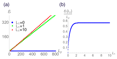
Figure 3: The entanglement negativity β„°β„°\mathcal{E} for two adjacent intervals (A1subscript𝐴1A_{1} and A2subscript𝐴2A_{2}) in the integer quantum Hall state on a cylinder. The length of subsystem A2subscript𝐴2A_{2} is L1subscript𝐿1L_{1} and the compactified length on the cylinder is Lysubscript𝐿𝑦L_{y}. (a) ℰ​(Ly)β„°subscript𝐿𝑦\mathcal{E}(L_{y}) for L1=0subscript𝐿10L_{1}=0 (Blue), L1=1subscript𝐿11L_{1}=1 (Green), and L1=10subscript𝐿110L_{1}=10 (Red). (b) ℰ​(Ly)Lyβ„°subscript𝐿𝑦subscript𝐿𝑦\frac{\mathcal{E}(L_{y})}{L_{y}} as a function of L1subscript𝐿1L_{1}. We set Lx=100​πsubscript𝐿π‘₯100πœ‹L_{x}=100\pi that particles are restricted in the region xβ©½|Lx/2|π‘₯subscript𝐿π‘₯2x\leqslant|L_{x}/2|.

The entanglement negativity is linearly proportional to Lysubscript𝐿𝑦L_{y} [Fig. 3 (a)], i.e., an area law behavior. For L1=0subscript𝐿10L_{1}=0, the dimension of Hilbert space of region A2subscript𝐴2A_{2} is zero that leads to the vanishing of the entanglement negativity. In the limit that L1β‰ͺLxmuch-less-thansubscript𝐿1subscript𝐿π‘₯L_{1}\ll L_{x}, the entanglement negativity increases monotonically as L1subscript𝐿1L_{1} increasing. Notice that when L1>Lxsubscript𝐿1subscript𝐿π‘₯L_{1}>L_{x}, all the particles are restricted in the subsystem A2subscript𝐴2A_{2}. Hence the entanglement negativity goes to zero. The slope of the entanglement computed from Eq. (45) is shown in Fig. 3 (b). The plateau of ℰ​(Ly)Lyβ„°subscript𝐿𝑦subscript𝐿𝑦\frac{\mathcal{E}(L_{y})}{L_{y}} is around 0.560.560.56, which indicates the system approaches to the case of a pure state when L1≫1much-greater-thansubscript𝐿11L_{1}\gg 1. We demonstrate the case of a pure state in the IQHS in the Appendix. A.2.

Disjointed intervals

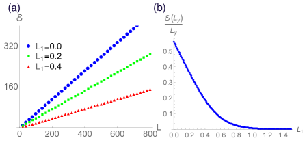
In Fig. 4 (a), the entanglement negativity also shows an area law behavior as the case of adjacent intervals. For L1=0subscript𝐿10L_{1}=0, the dimension of Hilbert space of region B𝐡B is zero. Hence the entanglement negativity is exact the same as the entanglement negativity for a pure state. As L1subscript𝐿1L_{1} is increasing, the entanglement negativity decreases. This indicates that A1subscript𝐴1A_{1} and A2subscript𝐴2A_{2} become less entangled when the distance between these two intervals becomes larger. The slope of the entanglement computed from Eq. (45) is shown in Fig. 4 (b). When L1=0subscript𝐿10L_{1}=0, the system can be described by a pure state and ℰ​(Ly)Ly∼0.56​⋯similar-toβ„°subscript𝐿𝑦subscript𝐿𝑦0.56β‹―\frac{\mathcal{E}(L_{y})}{L_{y}}\sim 0.56\cdots. Since the decay length in the system is proportional to lBsubscript𝑙𝐡l_{B}, A1subscript𝐴1A_{1} and A2subscript𝐴2A_{2} become less entangled when the distance between two disjointed intervals L1subscript𝐿1L_{1} is greater then lBsubscript𝑙𝐡l_{B}. We find that ℰ​(Ly)Lyβ„°subscript𝐿𝑦subscript𝐿𝑦\frac{\mathcal{E}(L_{y})}{L_{y}} monotonically decreases as L1subscript𝐿1L_{1} is increasing.

Refer to caption
Figure 4: The entanglement negativity β„°β„°\mathcal{E} for two disjointed intervals (A1subscript𝐴1A_{1} and A2subscript𝐴2A_{2}) in the integer quantum Hall state on a cylinder. The length of subsystem B𝐡B and the compactified length on on the cylinder is Lysubscript𝐿𝑦L_{y}. (a) ℰ​(Ly)β„°subscript𝐿𝑦\mathcal{E}(L_{y}) for L1=0subscript𝐿10L_{1}=0 (blue), L1=0.2subscript𝐿10.2L_{1}=0.2 (green), and L1=0.4subscript𝐿10.4L_{1}=0.4 (red). (b) ℰ​(Ly)Lyβ„°subscript𝐿𝑦subscript𝐿𝑦\frac{\mathcal{E}(L_{y})}{L_{y}} as a function of L1subscript𝐿1L_{1}. We set Lx=100​πsubscript𝐿π‘₯100πœ‹L_{x}=100\pi that particles are restricted in the region xβ©½|Lx/2|π‘₯subscript𝐿π‘₯2x\leqslant|L_{x}/2|.

III.1.3 Discussion

For the IQHS, as the distance L1subscript𝐿1L_{1} is larger than the magnetic length lB=1subscript𝑙𝐡1l_{B}=1, the entanglement negativity vanishes dramatically. It may be straightforwardly understood in the following. As studied in Ref. [Qi2011, ], for a (2+1) dimensional topological quantum state which possesses chiral edge states, such as the IQHS we discussed here, the reduced density matrix of a spatial region can be expressed as the density matrix of the corresponding edge states. In other words, the entanglement is mainly contributed by the boundary states which are localized at the interface. Therefore, for the configuration in Fig. 2, the reduced density matrix ρA1βˆͺA2subscript𝜌subscript𝐴1subscript𝐴2\rho_{A_{1}\cup A_{2}} can be expressed as

ρA1βˆͺA2=Οβˆ‚A1βŠ—Οβˆ‚A2,subscript𝜌subscript𝐴1subscript𝐴2tensor-productsubscript𝜌subscript𝐴1subscript𝜌subscript𝐴2\rho_{A_{1}\cup A_{2}}=\rho_{\partial A_{1}}\otimes\rho_{\partial A_{2}}, (46)

where Οβˆ‚Aisubscript𝜌subscript𝐴𝑖\rho_{\partial A_{i}} represents the density matrix corresponding to the boundary states located at the interface βˆ‚Aisubscript𝐴𝑖\partial A_{i} between region Aisubscript𝐴𝑖A_{i} and region B𝐡B. In this case, one has

ρA1βˆͺA2T2=Οβˆ‚A1βŠ—Οβˆ‚A2T,superscriptsubscript𝜌subscript𝐴1subscript𝐴2subscript𝑇2tensor-productsubscript𝜌subscript𝐴1superscriptsubscript𝜌subscript𝐴2𝑇\rho_{A_{1}\cup A_{2}}^{T_{2}}=\rho_{\partial A_{1}}\otimes\rho_{\partial A_{2}}^{T}, (47)

which leads to a vanishing entanglement negativity. Our conclusion also applies to a general topological ordered states such as the fractional quantum hall effect. The topological flux threading through the cylinder in Fig. 2 can be in a superposition of different topological sectors, and the reduced density matrix has the expression

ρA1βˆͺA2=βˆ‘a|ψa|2β€‹Οβˆ‚A1aβŠ—Οβˆ‚A2a,subscript𝜌subscript𝐴1subscript𝐴2subscriptπ‘Žtensor-productsuperscriptsubscriptπœ“π‘Ž2superscriptsubscript𝜌subscript𝐴1π‘Žsuperscriptsubscript𝜌subscript𝐴2π‘Ž\rho_{A_{1}\cup A_{2}}=\sum_{a}|\psi_{a}|^{2}\rho_{\partial A_{1}}^{a}\otimes\rho_{\partial A_{2}}^{a}, (48)

where |ψa|2superscriptsubscriptπœ“π‘Ž2|\psi_{a}|^{2} is the probability corresponding to the topological sector aπ‘Ža. Again, the state is explicitly separable, and therefore the entanglement negativity is zero. Note that the above conclusion was also obtained in Ref. [Lee, ] based on the solvable toric code mode, but here we give an argument which holds for a general topological ordered state in (2+1)D. A more strict proof based on the boundary state picture can be found in Ref. [Wen2015, ]. What ia interesting, most recently, the mutual information between A1subscript𝐴1A_{1} and A2subscript𝐴2A_{2} in Fig. 2 for a (2+1) dimensional topological ordered state was studied Qi2015 . It was found that

IA1​A2=βˆ’βˆ‘a|ψa|2​ln​|ψa|2,subscript𝐼subscript𝐴1subscript𝐴2subscriptπ‘Žsuperscriptsubscriptπœ“π‘Ž2lnsuperscriptsubscriptπœ“π‘Ž2I_{A_{1}A_{2}}=-\sum_{a}|\psi_{a}|^{2}\mathrm{ln}|\psi_{a}|^{2}, (49)

which is nonzero. One may understand the difference between the entanglement negativity and the mutual information in the following way. As pointed out in Ref. [Qi2015, ], the nonzero contribution in Eq. (49) comes from the β€œclassical” correlation between extended objects. It is known that the mutual information contains both classical and quantum correlations, while the entanglement negativity measures the completely quantum part of correlationsQiEmail ; Castelnovo . Therefore, one may have a vanishing entanglement negativity while the mutual information is finite.

III.2 The ground state in a tripartite system cannot be factored into triples of modes

For the case where the overlap matrices cannot be simultaneous diagonalized in a tripartite system, the ground state cannot be factorized. Although the ground state cannot be factorized, we can express the ground state in terms of the fermion operators in each subsystem. The procedure of constructing the ground state is the following. We start with the bipartite ground state

|Ψ⟩=ketΞ¨absent\displaystyle|\Psi\rangle= ∏i=1N(Pi​dA​i†+1βˆ’Pi​dB​i†)​|0⟩.superscriptsubscriptproduct𝑖1𝑁subscript𝑃𝑖subscriptsuperscript𝑑†𝐴𝑖1subscript𝑃𝑖subscriptsuperscript𝑑†𝐡𝑖ket0\displaystyle\prod_{i=1}^{N}(\sqrt{P_{i}}d^{\dagger}_{Ai}+\sqrt{1-P_{i}}d^{\dagger}_{Bi})|0\rangle. (50)

The orthonormal modes at A𝐴A are the set {|Ai⟩;dA​i†​|0⟩=|Ai⟩}ketsubscript𝐴𝑖superscriptsubscript𝑑𝐴𝑖†ket0ketsubscript𝐴𝑖\{|A_{i}\rangle;d_{Ai}^{\dagger}|0\rangle=|A_{i}\rangle\}. Next, we use these orthonormal modes in subsystem A𝐴A to construct the overlap matrices MA1subscript𝑀subscript𝐴1M_{A_{1}} and MA2subscript𝑀subscript𝐴2M_{A_{2}},

[MAi]Ξ±,Ξ²=βŸ¨π’«Ai​AΞ±,𝒫Ai​Aβ⟩,i=1,2,formulae-sequencesubscriptdelimited-[]subscript𝑀subscript𝐴𝑖𝛼𝛽subscript𝒫subscript𝐴𝑖subscript𝐴𝛼subscript𝒫subscript𝐴𝑖subscript𝐴𝛽𝑖12\displaystyle[M_{A_{i}}]_{\alpha,\beta}=\langle\mathcal{P}_{A_{i}}A_{\alpha},\mathcal{P}_{A_{i}}A_{\beta}\rangle,\quad i=1,2, (51)

where 𝒫Aisubscript𝒫subscript𝐴𝑖\mathcal{P}_{A_{i}} is the orthogonal projection operator on Hilbert space Aisubscript𝐴𝑖A_{i}. In other words, the tripartite system is built from partitioning the system into A𝐴A and B𝐡B parts first, and partitioning the subsystem A𝐴A into A1subscript𝐴1A_{1} and A2subscript𝐴2A_{2} parts. Since {|Ai⟩}ketsubscript𝐴𝑖\{|A_{i}\rangle\} is the orthonormal set, we have MA1+MA2=𝕀subscript𝑀subscript𝐴1subscript𝑀subscript𝐴2𝕀M_{A_{1}}+M_{A_{2}}=\mathbb{I}. We can simultaneously diagonalize MA1subscript𝑀subscript𝐴1M_{A_{1}} and MA2subscript𝑀subscript𝐴2M_{A_{2}} by a unitary matrix V𝑉V, such that V​MA1​V†=diag​(Qk)𝑉subscript𝑀subscript𝐴1superscript𝑉†diagsubscriptQkVM_{A_{1}}V^{\dagger}=\rm{diag}(Q_{k}) and V​MA2​V†=diag​(1βˆ’Qk)𝑉subscript𝑀subscript𝐴2superscript𝑉†diag1subscriptQkVM_{A_{2}}V^{\dagger}=\rm{diag}(1-Q_{k}). The orthonormal modes in A1subscript𝐴1A_{1} and A2subscript𝐴2A_{2} are

|A1​k⟩=Vk​i†​𝒫A1​|Ai⟩Qk,|A2​k⟩=Vk​i†​𝒫A2​|Ai⟩1βˆ’Qk.formulae-sequenceketsubscript𝐴1π‘˜subscriptsuperscriptπ‘‰β€ π‘˜π‘–subscript𝒫subscript𝐴1ketsubscript𝐴𝑖subscriptπ‘„π‘˜ketsubscript𝐴2π‘˜subscriptsuperscriptπ‘‰β€ π‘˜π‘–subscript𝒫subscript𝐴2ketsubscript𝐴𝑖1subscriptπ‘„π‘˜\displaystyle|A_{1k}\rangle=\frac{V^{\dagger}_{ki}\mathcal{P}_{A_{1}}|A_{i}\rangle}{\sqrt{Q_{k}}},\quad|A_{2k}\rangle=\frac{V^{\dagger}_{ki}\mathcal{P}_{A_{2}}|A_{i}\rangle}{\sqrt{1-Q_{k}}}. (52)

Now the ground state can be expressed as

|Ψ⟩=ketΞ¨absent\displaystyle|\Psi\rangle= ∏i=1N(Pi​dA​i†+1βˆ’Pi​dB​i†)​|0⟩superscriptsubscriptproduct𝑖1𝑁subscript𝑃𝑖subscriptsuperscript𝑑†𝐴𝑖1subscript𝑃𝑖subscriptsuperscript𝑑†𝐡𝑖ket0\displaystyle\prod_{i=1}^{N}(\sqrt{P_{i}}d^{\dagger}_{Ai}+\sqrt{1-P_{i}}d^{\dagger}_{Bi})|0\rangle
=\displaystyle= ∏i=1N(Piβˆ‘kVi​k(QkdA1​k†+1βˆ’QkdA2​k†)\displaystyle\prod_{i=1}^{N}(\sqrt{P_{i}}\sum_{k}V_{ik}(\sqrt{Q_{k}}d^{\dagger}_{A_{1}k}+\sqrt{1-Q_{k}}d^{\dagger}_{A_{2}k})
+1βˆ’PidB​i†)|0⟩,\displaystyle+\sqrt{1-P_{i}}d^{\dagger}_{Bi})|0\rangle, (53)

where dAi​k†​|0⟩=|Ai​k⟩superscriptsubscript𝑑subscriptπ΄π‘–π‘˜β€ ket0ketsubscriptπ΄π‘–π‘˜d_{A_{i}k}^{\dagger}|0\rangle=|A_{ik}\rangle with i=1,2𝑖12i=1,2. The second line in the above equation comes from

dA​i†​|0⟩subscriptsuperscript𝑑†𝐴𝑖ket0\displaystyle d^{\dagger}_{Ai}|0\rangle =|Ai⟩=𝒫A1​|Ai⟩+𝒫A2​|Ai⟩absentketsubscript𝐴𝑖subscript𝒫subscript𝐴1ketsubscript𝐴𝑖subscript𝒫subscript𝐴2ketsubscript𝐴𝑖\displaystyle=|A_{i}\rangle=\mathcal{P}_{A_{1}}|A_{i}\rangle+\mathcal{P}_{A_{2}}|A_{i}\rangle
=βˆ‘kVi​k​(Qk​dA1​k†+1βˆ’Qk​dA2​k†)​|0⟩.absentsubscriptπ‘˜subscriptπ‘‰π‘–π‘˜subscriptπ‘„π‘˜subscriptsuperscript𝑑†subscript𝐴1π‘˜1subscriptπ‘„π‘˜subscriptsuperscript𝑑†subscript𝐴2π‘˜ket0\displaystyle=\sum_{k}V_{ik}(\sqrt{Q_{k}}d^{\dagger}_{A_{1}k}+\sqrt{1-Q_{k}}d^{\dagger}_{A_{2}k})|0\rangle. (54)

In terms of occupation basis, the ground state can be expressed as

|Ψ⟩=βˆ‘n=0NCn​|nA,(Nβˆ’n)B⟩,ketΞ¨superscriptsubscript𝑛0𝑁subscript𝐢𝑛ketsubscript𝑛𝐴subscript𝑁𝑛𝐡\displaystyle|\Psi\rangle=\sum_{n=0}^{N}C_{n}|n_{A},(N-n)_{B}\rangle, (55)

where nAsubscript𝑛𝐴n_{A} indicates that there are n𝑛n electrons in subsystem A=A1βˆͺA2𝐴subscript𝐴1subscript𝐴2A=A_{1}\cup A_{2} and (Nβˆ’n)Bsubscript𝑁𝑛𝐡(N-n)_{B} indicates that there are Nβˆ’n𝑁𝑛N-n electrons in subsystem B𝐡B. We can construct the partially transposed reduced density matrix from the occupational basis [see detail derivations in App. B]. The final expression of ρATA2superscriptsubscript𝜌𝐴subscript𝑇subscript𝐴2\rho_{A}^{T_{A_{2}}} is

ρATA2=βˆ‘ni=11,00,10,01Cn1,n2,β‹―,nN​⨂i=1N[ρni]iTA2,superscriptsubscript𝜌𝐴subscript𝑇subscript𝐴2subscriptsubscript𝑛𝑖11001001subscript𝐢subscript𝑛1subscript𝑛2β‹―subscript𝑛𝑁superscriptsubscripttensor-product𝑖1𝑁subscriptsuperscriptdelimited-[]subscript𝜌subscript𝑛𝑖subscript𝑇subscript𝐴2𝑖\displaystyle\rho_{A}^{T_{A_{2}}}=\sum_{n_{i}=11,00,10,01}C_{n_{1},n_{2},\cdots,n_{N}}\bigotimes_{i=1}^{N}[\rho_{n_{i}}]^{T_{A_{2}}}_{i}, (56)

where ρnisubscript𝜌subscript𝑛𝑖\rho_{n_{i}} are four elemental matrices (see Eq. (92) in App. B) as the building blocks of ρATA2superscriptsubscript𝜌𝐴subscript𝑇subscript𝐴2\rho_{A}^{T_{A_{2}}}. Thus, the entanglement negativity can be obtained by taking the trace norm, β„°=ln⁑Tr​|ρATA2|β„°Trsuperscriptsubscript𝜌𝐴subscript𝑇subscript𝐴2\mathcal{E}=\ln\mathrm{Tr}|\rho_{A}^{T_{A_{2}}}|.

III.2.1 Free fermions on a 1D ring

Refer to caption
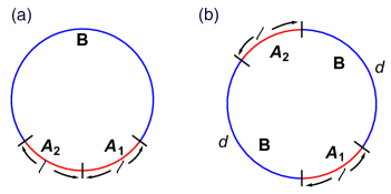
Figure 5: Two tripartite configurations of 1D rings: (a) Two adjacent intervals A1subscript𝐴1A_{1} and A2subscript𝐴2A_{2} with equal length l𝑙l. (b) Two disjointed intervals A1subscript𝐴1A_{1} and A2subscript𝐴2A_{2} with equal length l𝑙l and the length between these two intervals is d𝑑d.

We consider free fermions on a periodic one-dimensional chain. The normalized single-particle eigenstate is

Ο•n=1L​ei​2​n​πL​x,nβˆˆβ„€,formulae-sequencesubscriptitalic-ϕ𝑛1𝐿superscript𝑒𝑖2π‘›πœ‹πΏπ‘₯𝑛℀\displaystyle\phi_{n}=\frac{1}{\sqrt{L}}e^{i\frac{2n\pi}{L}x},\quad n\in\mathbb{Z}, (57)

with energy En=(2​π​nL)2subscript𝐸𝑛superscript2πœ‹π‘›πΏ2E_{n}=(\frac{2\pi n}{L})^{2}. The overlap matrix can be constructed from these eigenstates from Eq. (5) and the partially transposed reduced density matrix can be obtained from Eq. (112).

Due to the limitation of numerical calculation, we consider few fermions (up to five) on a long chain (L>50𝐿50L>50). For simplicity, two intervals A1subscript𝐴1A_{1} and A2subscript𝐴2A_{2} have equal length l𝑙l and the total length of the ring is L𝐿L.

Adjacent intervals
Refer to caption
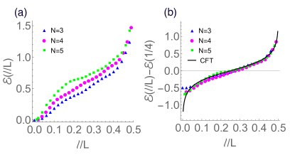
Figure 6: (a) The entanglement negativity ℰ​(l/L)ℰ𝑙𝐿\mathcal{E}(l/L) as a function of l/L𝑙𝐿l/L for two adjacent intervals in a homogeneous one-dimensional ring with N𝑁N particles. Two intervals are equal length l𝑙l and the total length of the ring is L𝐿L. (b) ℰ​(l/L)βˆ’β„°β€‹(1/4)ℰ𝑙𝐿ℰ14\mathcal{E}(l/L)-\mathcal{E}(1/4) as a function of l/L𝑙𝐿l/L. Solid grey line is the scaling function from CFT calculation, β„°=14ln[tan(Ο€lL))]\mathcal{E}=\frac{1}{4}\mathrm{ln[tan}(\pi\frac{l}{L}))].

The configuration of adjacent intervals is shown in Fig. 5(a). For fixed number of particles, the entanglement negativity of adjacent intervals depends on the single parameter l/L𝑙𝐿l/L. The entanglement negativity increases monotonically as the function of l/L𝑙𝐿l/L [Fig. 6 (a)]. In the CFT calculationCalabrese ; Calabrese2 , β„°=14ln[tan(Ο€lL))]+const.\mathcal{E}=\frac{1}{4}\mathrm{ln[tan}(\pi\frac{l}{L}))]+\mathrm{const.}. In order to compare with the CFT calculation and get rid of the constant part in the entanglement negativity, we plot ℰ​(l/L)βˆ’β„°β€‹(1/4)ℰ𝑙𝐿ℰ14\mathcal{E}(l/L)-\mathcal{E}(1/4) for N=3,4,5𝑁345N=3,4,5. in Fig. 6 (b). The entanglement negativity after the subtraction of ℰ​(1/4)β„°14\mathcal{E}(1/4) agrees with the CFT prediction.

Disjointed intervals

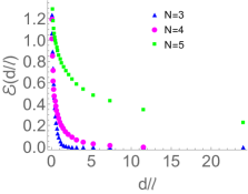
The entanglement negativity of disjointed intervals for harmonic chains has been studied in Refs. [Wichterich2, ; Marcovitch, ; Calabrese, ]. Here, we consider a symmetric configuration of disjointed intervals as shown in Fig. 5(b). For fixed number of particles, the entanglement negativity of disjointed intervals depends on the single parameter d/l𝑑𝑙d/l, where d𝑑d is the distance between two intervals. The entanglement negativity decreases monotonically as the function of d/l𝑑𝑙d/l [Fig. 7].

Refer to caption
Figure 7: The entanglement negativity ℰ​(d/l)ℰ𝑑𝑙\mathcal{E}(d/l) as a function of d/l𝑑𝑙d/l for two disjointed intervals in a homogeneous one-dimensional ring with N𝑁N particles. Two disjointed intervals have equal length l𝑙l and the distance between two intervals is d𝑑d.

IV Discussion and conclusion

In this paper, we systematically derive the entanglement negativity in free-fermion systems by using the overlap matrices. For a pure state, the entanglement negativity is obtained from a bipartite system and the ground state can always be factored into pairs of modes. For a mixed state, the factorability of the ground state in a tripartite system does not always hold. In the case that the ground state can still be factored into triples of modes, the entanglement negativity has a simple form. We show two examples in this case: the dimerized SSH model and the IQHS. The entanglement negativity for the former is ln⁑22\ln 2 when two intervals are adjacent. The entanglement negativity for the latter shows an area law behavior. For both examples, we observe that the entanglement negativity vanishes when the separation between two intervals is greater than the correlation length of the systems. We argue the vanish of the entanglement negativity holds for a general topological ordered state in (2+1)21(2+1)D. A proof based on the edge theory approach as well as the bulk theory calculation is given in Refs. [Wen2015, ] and Ref. [EN_CS, ], respectively. On the other hand, if the ground state cannot be factored into triples of modes, we show that the partially transposed reduced density matrix can be expressed in terms of the Kronecker product of matrices. In this case, we compute the entanglement negativity for free fermions on a one-dimensional ring. We find that the entanglement negativity of two adjacent intervals agrees with the CFT prediction.

We would like to end the conclusion by mentioning a few of future problems.

βˆ™βˆ™\bullet It is interesting to study the non-equilibrium dynamics of entanglement negativity for a free-fermion system. In particular, as discussed in Ref. [Wen, ], for the time evolution of entanglement negativity ℰ​(t)ℰ𝑑\mathcal{E}(t) after a local quench, the result is not universal for some region t𝑑t, i.e., ℰ​(t)ℰ𝑑\mathcal{E}(t) may depend on the concrete lattice models. It is interesting to check the behavior of ℰ​(t)ℰ𝑑\mathcal{E}(t) for a critical free fermion chain, and compare it with the results of other lattice models Eisler .

βˆ™βˆ™\bullet In our current work, we mainly focus on the free-fermion systems at zero temperature. It is desirable to generalize our method to the finite temperature case, and compare with the CFT resultsCalabrese4 .

βˆ™βˆ™\bullet One can easily apply our methods to free-fermion systems with disorder. Studying the quantum phase transitions of disordered systems by using the entanglement negativity is needed for a future investigation.

βˆ™βˆ™\bullet It is interesting to extend our method to the study of interacting fermionic systems, such as fractional quantum hall systems. Although there is no entanglement negativity for two disjoint intervals, it is still interesting to study the entanglement negativity for two adjacent intervals, where we may have a nonvanishing contribution from the long-range entanglement.

V Acknowledgement

The authors thank Shinsei Ryu for his encouragement and discussions during this work. PYC is supported by the Rutgers Center for Materials Theory group postdoc grant.

References

  • (1) G. Vidal, J. I. Latorre, E. Rico, and A. Kitaev, Phys. Rev. Lett. 90, 227902 (2003).
  • (2) P. Calabrese and J. Cardy, J. Stat. Mech. P06002 (2004).
  • (3) A. Kitaev and J. Preskill, Phys. Rev. Lett. 96, 110404 (2006).
  • (4) M. Levin and X.-G. Wen, Phys. Rev. Lett. 96, 110405 (2006).
  • (5) L. Amico, R. Fazio, A. Osterloh, and V. Vedral, Rev. Mod. Phys. 80, 517 (2008);
  • (6) P. Calabrese and J. Cardy, J. of Phys. A: Math. and Theor. 42, 504005 (2009).
  • (7) P. Calabrese, J. Cardy, and B. Doyon Eds, J. Phys. A 42 500301 (2009).
  • (8) J. Eisert, M. Cramer, and M. B. Plenio, Rev. Mod. Phys. 82, 277 (2010).
  • (9) F. Benatti, R. Floreanini, and U. Marzolino, Ann. Phys. 327, 1304 (2012).
  • (10) F. Benatti, R. Floreanini, and U. Marzolino, Phys. Rev. A 89, 032326 (2014).
  • (11) J. Eisert and M. B. Plenio, J. Mod. Opt. 46, 145 (1999).
  • (12) G. Vidal and R. F. Werner, Phys. Rev. A 65, 032314 (2002).
  • (13) M.B. Plenio Phys. Rev. Lett. 95, 090503 (2005).
  • (14) P. Calabrese, J. Cardy, and E. Tonni, J. Stat. Mech. P02008 (2013).
  • (15) P. Calabrese, J. Cardy, and E. Tonni, Phys. Rev. Lett. 109, 130502 (2012).
  • (16) K. Audenaert, J. Eisert, M. B. Plenio, and R. F. Werner, Phys. Rev. A 66, 042327 (2002).
  • (17) A. Ferraro, D. Cavalcanti, A. GarcΓ­a-Saez, and A. AcΓ­n, Phys. Rev. Lett. 100, 080502 (2008).
  • (18) D. Cavalcanti, A. Ferraro, A. GarcΓ­a-Saez, and A. AcΓ­n, Phys. Rev. A 78, 012335 (2008).
  • (19) J. Anders and A. Winter, Quantum Inf. Comput. 8, 0245 (2008).
  • (20) J. Anders, Phys. Rev. A 77, 062102 (2008).
  • (21) S. Marcovitch, A. Retzker, M. B. Plenio, and B. Reznik, Phys. Rev. A 80, 012325 (2009).
  • (22) H. Wichterich, J. Molina-Vilaplana, and S. Bose Phys. Rev. A 80, 010304(R) (2009).
  • (23) H. Wichterich, J. Vidal, and S. Bose, Phys. Rev. A 81, 032311 (2010).
  • (24) A. Bayat, S. Bose, and P. Sodano, Phys. Rev. Lett. 105, 187204 (2010).
  • (25) A. Bayat, P. Sodano, and S. Bose, Phys. Rev. B 81, 064429 (2010).
  • (26) A. Bayat, S. Bose, P. Sodano, and H. Johannesson, Phys. Rev. Lett. 109, 066403 (2012).
  • (27) R. A. Santos, V. Korepin, and S. Bose, Phys. Rev. A 84, 062307 (2011).
  • (28) C. Castelnovo, Phys. Rev. A 88, 042319 (2013).
  • (29) Y. A. Lee and G. Vidal, Phys. Rev. A 88, 042318 (2013).
  • (30) X. Wen, P.-Y. Chang, and S. Ryu,to appear.
  • (31) P. Calabrese, L. Tagliacozzo, and E. Tonni, J. Stat. Mech. P05002 (2013).
  • (32) V. Alba, J. Stat. Mech. P05013 (2013).
  • (33) C.-M. Chung, V. Alba, L. Bonnes, P. Chen, and A. M. LΓ€uchli, Phys. Rev. B 90, 064401 (2014).
  • (34) C. D. Nobili, A. Coser, E. Tonni, J. Stat. Mech. P06021 (2015).
  • (35) V. Eisler and Z. ZimborΓ‘s, New J. Phys. 16, 123020 (2014).
  • (36) A. Coser, E. Tonni, and P. Calabrese, J. Stat. Mech P12017 (2014).
  • (37) M. Hoogeveen and B. Doyon, Nucl. Phys. B 898, 78 (2015).
  • (38) X. Wen, P.-Y. Chang, and S. Ryu, Phys. Rev. B 92, 075109 (2015).
  • (39) P. Calabrese, J. Cardy, and E. Tonni, J. Phys. A 48, 015006 (2015).
  • (40) V. Eisler and Z. ZimborΓ‘s, New J. Phys. 17, 053048 (2015).
  • (41) A. Coser, E. Tonni, P. Calabrese, J. Stat. Mech. P08005 (2015).
  • (42) A. Coser, E. Tonni, P. Calabrese, J.Stat.Mech. 033116 (2016).
  • (43) V. Eisler and Z. ZimborΓ‘s, Phys. Rev. B 93,115148 (2016).
  • (44) A. Coser, E. Tonni, P. Calabrese, arXiv:1511.08328.
  • (45) I. Klich, J. Phys. A: Math. Gen. 39, L85-L91 (2006).
  • (46) P Calabrese, M. Mintchev, and E. Vicari, Phys. Rev. Lett. 107, 020601 (2011).
  • (47) P. Calabrese, M. Mintchev, E. Vicari, J. Stat. Mech. P09028 (2011).
  • (48) P. Calabrese, M. Mintchev and E. Vicari, EPL 97 20009 (2012).
  • (49) A. Ossipov Phys. Rev. Lett. 113, 130402 (2014).
  • (50) J. E. Drut, W. J. Porter, arXiv:1510.01723.
  • (51) W. P. Su, J. R. Schrieffer, and A. J. Heeger, Phys. Rev. Lett. 42, 1698 (1979).
  • (52) I. D. RodrΓ­guez and G. Sierra, Phys. Rev. B, 80 153303 (2009).
  • (53) P.-Y. Chang, C. Mudry, and S. Ryu, J. Stat. Mech. P09014 (2014).
  • (54) X-L Qi, H. Katsura, and A. W. W. Ludwig, Phys. Rev. Lett. 108, 196402 (2012)
  • (55) X. Wen, S. Matsuura, and Shinsei Ryu, arXiv:1603.08534
  • (56) C-M Jian, I. H. Kim, and X-L Qi, arXiv:1508.07006
  • (57) We thank Xiao-Liang Qi for comments on this issue.

Appendix A Entanglement negativity for pure states

Let us consider a bipartite system that the ground state can be Schmidt decomposed as

|Ψ⟩=βˆ‘iCi​|ψA​iβ€‹ΟˆB​i⟩,ketΞ¨subscript𝑖subscript𝐢𝑖ketsubscriptπœ“π΄π‘–subscriptπœ“π΅π‘–\displaystyle|\Psi\rangle=\sum_{i}C_{i}|\psi_{Ai}\psi_{Bi}\rangle, (58)

where Cisubscript𝐢𝑖C_{i} is the coefficient that in between zero and one and the system is bipartite into A and B parts. The density matrix and the reduced density matrix are defined as

ρ=|Ξ¨βŸ©β€‹βŸ¨Ξ¨|=βˆ‘i,jCi​Cj​|ψA​iβ€‹ΟˆB​iβŸ©β€‹βŸ¨ΟˆA​jβ€‹ΟˆB​j|,𝜌ketΞ¨braΞ¨subscript𝑖𝑗subscript𝐢𝑖subscript𝐢𝑗ketsubscriptπœ“π΄π‘–subscriptπœ“π΅π‘–brasubscriptπœ“π΄π‘—subscriptπœ“π΅π‘—\displaystyle\rho=|\Psi\rangle\langle\Psi|=\sum_{i,j}C_{i}C_{j}|\psi_{Ai}\psi_{Bi}\rangle\langle\psi_{Aj}\psi_{Bj}|,
ρA=TrB​ρ=βˆ‘iCi2​|ψA​iβŸ©β€‹βŸ¨ΟˆA​i|.subscript𝜌𝐴subscriptTr𝐡𝜌subscript𝑖superscriptsubscript𝐢𝑖2ketsubscriptπœ“π΄π‘–brasubscriptπœ“π΄π‘–\displaystyle\rho_{A}=\mathrm{Tr}_{B}\rho=\sum_{i}C_{i}^{2}|\psi_{Ai}\rangle\langle\psi_{Ai}|. (59)

One can define a partial transpose of the density matrix as

ρTB=βˆ‘i,jCi​Cj​|ψA​iβ€‹ΟˆB​jβŸ©β€‹βŸ¨ΟˆA​jβ€‹ΟˆB​i|.superscript𝜌subscript𝑇𝐡subscript𝑖𝑗subscript𝐢𝑖subscript𝐢𝑗ketsubscriptπœ“π΄π‘–subscriptπœ“π΅π‘—brasubscriptπœ“π΄π‘—subscriptπœ“π΅π‘–\displaystyle\rho^{T_{B}}=\sum_{i,j}C_{i}C_{j}|\psi_{Ai}\psi_{Bj}\rangle\langle\psi_{Aj}\psi_{Bi}|. (60)

The trace norm of ρTBsuperscript𝜌subscript𝑇𝐡\rho^{T_{B}} is defined by

Tr​|ρTB|:=βˆ‘i|Ξ›i|,assignTrsuperscript𝜌subscript𝑇𝐡subscript𝑖subscriptΛ𝑖\displaystyle\mathrm{Tr}|\rho^{T_{B}}|:=\sum_{i}|\Lambda_{i}|, (61)

where Ξ›isubscriptΛ𝑖\Lambda_{i} is the eigenvalue of ρTBsuperscript𝜌subscript𝑇𝐡\rho^{T_{B}}.

The (logarithmic) entanglement negativity is defined as

β„°:=ln​Tr​|ρTB|.assignβ„°lnTrsuperscript𝜌subscript𝑇𝐡\displaystyle\mathcal{E}:=\mathrm{ln\,Tr}|\rho^{T_{B}}|. (62)

A.1 Su-Schrieffer-Heeger (SSH) model

Refer to caption
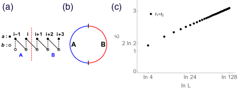
Figure 8: (a) Su-Schrieffer-Heeger model on a one-dimensional ring. The hopping amplitude of dashed(solid) lines is t1​(t2)subscript𝑑1subscript𝑑2t_{1}(t_{2}). A unit cell contains two orbitals that are pictured by βˆ™βˆ™\bullet and ∘\circ. The system is divided into A𝐴A and B𝐡B parts by the red dashed line. (b) The bipartite configuration of a ring with the lengths of A𝐴A and B𝐡B being equal. (c) The entanglement negativity β„°β„°\mathcal{E} for an equally bipartite Su-Schrieffer-Heeger model with t1=t2subscript𝑑1subscript𝑑2t_{1}=t_{2} as a function of ln​Lln𝐿\mathrm{ln}L, where L𝐿L is the length of the ring.

Let us consider an one-dimensional tight binding Hamiltonian (SSH model) under periodic boundary condition

H=βˆ‘it1​cai†​cbi+t2​cai+1†​cbi+h.c.formulae-sequence𝐻subscript𝑖subscript𝑑1subscriptsuperscript𝑐†subscriptπ‘Žπ‘–subscript𝑐subscript𝑏𝑖subscript𝑑2subscriptsuperscript𝑐†subscriptπ‘Žπ‘–1subscript𝑐subscript𝑏𝑖hc\displaystyle H=\sum_{i}t_{1}c^{\dagger}_{a_{i}}c_{b_{i}}+t_{2}c^{\dagger}_{a_{i+1}}c_{b_{i}}+\mathrm{h.c.}

where t1,t2>1subscript𝑑1subscript𝑑21t_{1},t_{2}>1 and ca​(b)isubscriptπ‘π‘Žsubscript𝑏𝑖c_{a(b)_{i}} is the fermion operator. The configuration of a bipartite ring is shown in Fig. 8. We consider the lengths of A𝐴A and B𝐡B are equal. The overlap matrix MAsubscript𝑀𝐴M_{A} has two eigenstates with 0.50.50.5 eigenvalue when t2>t1subscript𝑑2subscript𝑑1t_{2}>t_{1}. On the other hand, there is no eigenstates of MAsubscript𝑀𝐴M_{A} with 0.50.50.5 eigenvalue when t1>t2subscript𝑑1subscript𝑑2t_{1}>t_{2}. For t1=0subscript𝑑10t_{1}=0, the set of the eigenvalues of MAsubscript𝑀𝐴M_{A} is {Pi}={0,0,β‹―,0.5,0,5,1,1,β‹―,1}subscript𝑃𝑖00β‹―0.50511β‹―1\{P_{i}\}=\{0,0,\cdots,0.5,0,5,1,1,\cdots,1\}, that leads to β„°=2​l​n​2β„°2ln2\mathcal{E}=2\mathrm{ln}2. For t2=0subscript𝑑20t_{2}=0, the set of the entanglement spectrum is {Pi}={0,0,β‹―,0,1,β‹―,1}subscript𝑃𝑖00β‹―01β‹―1\{P_{i}\}=\{0,0,\cdots,0,1,\cdots,1\}. This implies β„°=0β„°0\mathcal{E}=0. At critical point, t1=t2subscript𝑑1subscript𝑑2t_{1}=t_{2}, the scaling function of the entanglement negativity is proportional to ln​Lln𝐿\mathrm{ln}L with L𝐿L being the length of the system. The set of points in Fig. 8(c) fits 0.71+0.50​x0.710.50π‘₯0.71+0.50x. From the CFT predictionCalabrese , the entanglement negativity is β„°=c2​ln⁑Lπ​sin⁑π​lL+const.ℰ𝑐2πΏπœ‹πœ‹π‘™πΏconst\mathcal{E}=\frac{c}{2}\ln\frac{L}{\pi}\sin\frac{\pi l}{L}+\mathrm{const.}. In our consideration, l/L=1/2𝑙𝐿12l/L=1/2, that leads to β„°=c2​ln⁑L+const.ℰ𝑐2𝐿const\mathcal{E}=\frac{c}{2}\ln L+\mathrm{const.}. One can read off the central charge c∼1similar-to𝑐1c\sim 1.

A.2 Integer Quantum Hall state (IQHS)

We consider the integer quantum Hall state (IQHS) on a cylinder. We choose the periodic boundary condition along y𝑦y direction. Hence kysubscriptπ‘˜π‘¦k_{y} is a good quantum number. The single-particle state in the lowest Landau level with the Landau gauge is

ψky​(x,y)=1Ο€1/4​Ly1/2​ei​ky​y​eβˆ’(xβˆ’lB2​ky)2/(2​lB2),subscriptπœ“subscriptπ‘˜π‘¦π‘₯𝑦1superscriptπœ‹14superscriptsubscript𝐿𝑦12superscript𝑒𝑖subscriptπ‘˜π‘¦π‘¦superscript𝑒superscriptπ‘₯superscriptsubscript𝑙𝐡2subscriptπ‘˜π‘¦22superscriptsubscript𝑙𝐡2\displaystyle\psi_{k_{y}}(x,y)=\frac{1}{\pi^{1/4}L_{y}^{1/2}}e^{ik_{y}y}e^{-(x-l_{B}^{2}k_{y})^{2}/(2l_{B}^{2})}, (64)

where

ky=βˆ’Lx2+n​π​lB2Ly,1β©½nβ©½Lx​Lyπ​lB2.formulae-sequencesubscriptπ‘˜π‘¦subscript𝐿π‘₯2π‘›πœ‹superscriptsubscript𝑙𝐡2subscript𝐿𝑦1𝑛subscript𝐿π‘₯subscriptπΏπ‘¦πœ‹superscriptsubscript𝑙𝐡2\displaystyle k_{y}=-\frac{L_{x}}{2}+n\frac{\pi l_{B}^{2}}{L_{y}},\quad 1\leqslant n\leqslant\frac{L_{x}L_{y}}{\pi l_{B}^{2}}. (65)

Here the number of particles Lx​Lyπ​lB2subscript𝐿π‘₯subscriptπΏπ‘¦πœ‹superscriptsubscript𝑙𝐡2\frac{L_{x}L_{y}}{\pi l_{B}^{2}} is obtained by restricting the particles in the region |x|β©½Lx/2π‘₯subscript𝐿π‘₯2|x|\leqslant L_{x}/2. Without loss of generality, we set the magnetic length lB=1subscript𝑙𝐡1l_{B}=1. The system is divided into A𝐴A and B𝐡B at x=0π‘₯0x=0, where A∈[βˆ’βˆž,0]𝐴0A\in[-\infty,0] and B∈[0,∞]𝐡0B\in[0,\infty] along xπ‘₯x axis. From Refs. [Ivan, ; Chang, ], the corresponding probabilities for a particle at region A𝐴A and B𝐡B are

PA=1Ο€β€‹βˆ«βˆ’βˆž0𝑑x​eβˆ’(xβˆ’ky)2=12​(1βˆ’erf​(ky)),subscript𝑃𝐴1πœ‹superscriptsubscript0differential-dπ‘₯superscript𝑒superscriptπ‘₯subscriptπ‘˜π‘¦2121erfsubscriptπ‘˜π‘¦\displaystyle P_{A}=\frac{1}{\sqrt{\pi}}\int_{-\infty}^{0}dxe^{-(x-k_{y})^{2}}=\frac{1}{2}(1-\mathrm{erf}(k_{y})),
PB=1Ο€β€‹βˆ«0βˆžπ‘‘x​eβˆ’(xβˆ’ky)2=12​(1+erf​(ky)).subscript𝑃𝐡1πœ‹superscriptsubscript0differential-dπ‘₯superscript𝑒superscriptπ‘₯subscriptπ‘˜π‘¦2121erfsubscriptπ‘˜π‘¦\displaystyle P_{B}=\frac{1}{\sqrt{\pi}}\int_{0}^{\infty}dxe^{-(x-k_{y})^{2}}=\frac{1}{2}(1+\mathrm{erf}(k_{y})). (66)

From Eq. (17), the entanglement negativity is

β„°=βˆ‘kyln​(1+1βˆ’erf​(ky)2).β„°subscriptsubscriptπ‘˜π‘¦ln11erfsuperscriptsubscriptπ‘˜π‘¦2\displaystyle\mathcal{E}=\sum_{k_{y}}\mathrm{ln}(1+\sqrt{1-\mathrm{erf}(k_{y})^{2}}). (67)

Numerically we observe that the entanglement negativity is linearly proportional to the length Lysubscript𝐿𝑦L_{y}. This indicates that the entanglement negativity satisfies an area law. The slope of the entanglement negativity can be obtained by taking the continuous limit

ℰ​(Ly)Lyβ„°subscript𝐿𝑦subscript𝐿𝑦\displaystyle\frac{\mathcal{E}(L_{y})}{L_{y}} =limLxβ†’βˆž1Ο€β€‹βˆ«βˆ’Lx/2Lx/2ln⁑[1+1βˆ’erf2​(ky)]​𝑑kyabsentsubscriptβ†’subscript𝐿π‘₯1πœ‹superscriptsubscriptsubscript𝐿π‘₯2subscript𝐿π‘₯211superscripterf2subscriptπ‘˜π‘¦differential-dsubscriptπ‘˜π‘¦\displaystyle=\lim_{L_{x}\to\infty}\frac{1}{\pi}\int_{-L_{x}/2}^{L_{x}/2}\ln[1+\sqrt{1-\mathrm{erf}^{2}(k_{y})}]dk_{y}
≃0.56​⋯.similar-to-or-equalsabsent0.56β‹―\displaystyle\simeq 0.56\cdots. (68)

Appendix B Detail expression of the partially transposed reduced density matrix for the non-triply factored case

In the main text, we can write down the ground state in a tripartite systems as,

|Ψ⟩=ketΞ¨absent\displaystyle|\Psi\rangle= ∏i=1N(Pi​dA​i†+1βˆ’Pi​dB​i†)​|0⟩superscriptsubscriptproduct𝑖1𝑁subscript𝑃𝑖subscriptsuperscript𝑑†𝐴𝑖1subscript𝑃𝑖subscriptsuperscript𝑑†𝐡𝑖ket0\displaystyle\prod_{i=1}^{N}(\sqrt{P_{i}}d^{\dagger}_{Ai}+\sqrt{1-P_{i}}d^{\dagger}_{Bi})|0\rangle
=\displaystyle= ∏i=1N(Piβˆ‘kVi​k(QkdA1​k†+1βˆ’QkdA2​k†)\displaystyle\prod_{i=1}^{N}(\sqrt{P_{i}}\sum_{k}V_{ik}(\sqrt{Q_{k}}d^{\dagger}_{A_{1}k}+\sqrt{1-Q_{k}}d^{\dagger}_{A_{2}k})
+1βˆ’PidB​i†)|0⟩,\displaystyle+\sqrt{1-P_{i}}d^{\dagger}_{Bi})|0\rangle, (69)

where Vi​ksubscriptπ‘‰π‘–π‘˜V_{ik} is a unitary matrix that can simultaneously diagonalize the overlap matrices MA1subscript𝑀subscript𝐴1M_{A_{1}} and MA2subscript𝑀subscript𝐴2M_{A_{2}} in region A=A1βˆͺA2𝐴subscript𝐴1subscript𝐴2A=A_{1}\cup A_{2}. In terms of occupation basis, the ground state can be expressed as

|Ψ⟩=βˆ‘n=0NCn​|nA,(Nβˆ’n)B⟩,ketΞ¨superscriptsubscript𝑛0𝑁subscript𝐢𝑛ketsubscript𝑛𝐴subscript𝑁𝑛𝐡\displaystyle|\Psi\rangle=\sum_{n=0}^{N}C_{n}|n_{A},(N-n)_{B}\rangle, (70)

where nAsubscript𝑛𝐴n_{A} indicates that there are n𝑛n electrons in subsystem A=A1βˆͺA2𝐴subscript𝐴1subscript𝐴2A=A_{1}\cup A_{2} and (Nβˆ’n)Bsubscript𝑁𝑛𝐡(N-n)_{B} indicates that there are Nβˆ’n𝑁𝑛N-n electrons in subsystem B𝐡B. We have

Cn​|nA,(Nβˆ’n)B⟩=subscript𝐢𝑛ketsubscript𝑛𝐴subscript𝑁𝑛𝐡absent\displaystyle C_{n}|n_{A},(N-n)_{B}\rangle= βˆ‘i1>i2>β‹―>inPi1​Pi2​⋯​Pinβ€‹βˆ‘k1>k2>β‹―>knDet​[V{i},{k}minor]subscriptsubscript𝑖1subscript𝑖2β‹―subscript𝑖𝑛subscript𝑃subscript𝑖1subscript𝑃subscript𝑖2β‹―subscript𝑃subscript𝑖𝑛subscriptsubscriptπ‘˜1subscriptπ‘˜2β‹―subscriptπ‘˜π‘›Detdelimited-[]subscriptsuperscript𝑉minorπ‘–π‘˜\displaystyle\sum_{i_{1}>i_{2}>\cdots>i_{n}}\sqrt{P_{i_{1}}}\sqrt{P_{i_{2}}}\cdots\sqrt{P_{i_{n}}}\sum_{k_{1}>k_{2}>\cdots>k_{n}}\mathrm{Det}[V^{\mathrm{minor}}_{\{i\},\{k\}}]
Γ—(Qk1​dA1​k1†+1βˆ’Qk1​dA2​k1†)​(Qk2​dA1​k2†+1βˆ’Qk2​dA2​k2†)​⋯absentsubscript𝑄subscriptπ‘˜1subscriptsuperscript𝑑†subscript𝐴1subscriptπ‘˜11subscript𝑄subscriptπ‘˜1subscriptsuperscript𝑑†subscript𝐴2subscriptπ‘˜1subscript𝑄subscriptπ‘˜2subscriptsuperscript𝑑†subscript𝐴1subscriptπ‘˜21subscript𝑄subscriptπ‘˜2subscriptsuperscript𝑑†subscript𝐴2subscriptπ‘˜2β‹―\displaystyle\times(\sqrt{Q_{k_{1}}}d^{\dagger}_{A_{1}k_{1}}+\sqrt{1-Q_{k_{1}}}d^{\dagger}_{A_{2}k_{1}})(\sqrt{Q_{k_{2}}}d^{\dagger}_{A_{1}k_{2}}+\sqrt{1-Q_{k_{2}}}d^{\dagger}_{A_{2}k_{2}})\cdots
Γ—(Qkn​dA1​kn†+1βˆ’Qkn​dA2​kn†)β€‹βˆΞ±β‰ i1,i2,β‹―,in1βˆ’Pα​dB​α†​|0⟩,absentsubscript𝑄subscriptπ‘˜π‘›subscriptsuperscript𝑑†subscript𝐴1subscriptπ‘˜π‘›1subscript𝑄subscriptπ‘˜π‘›subscriptsuperscript𝑑†subscript𝐴2subscriptπ‘˜π‘›subscriptproduct𝛼subscript𝑖1subscript𝑖2β‹―subscript𝑖𝑛1subscript𝑃𝛼subscriptsuperscript𝑑†𝐡𝛼ket0\displaystyle\times(\sqrt{Q_{k_{n}}}d^{\dagger}_{A_{1}k_{n}}+\sqrt{1-Q_{k_{n}}}d^{\dagger}_{A_{2}k_{n}})\prod_{\alpha\neq i_{1},i_{2},\cdots,i_{n}}\sqrt{1-P_{\alpha}}d^{\dagger}_{B\alpha}|0\rangle, (71)

where Det​[V{i},{k}minor]Detdelimited-[]subscriptsuperscript𝑉minorπ‘–π‘˜\mathrm{Det}[V^{\mathrm{minor}}_{\{i\},\{k\}}] is the determinant of the unitary matrix V𝑉V by picking i1,i2,β‹―,insubscript𝑖1subscript𝑖2β‹―subscript𝑖𝑛i_{1},i_{2},\cdots,i_{n}-th rows and k1,k2,β‹―,knsubscriptπ‘˜1subscriptπ‘˜2β‹―subscriptπ‘˜π‘›k_{1},k_{2},\cdots,k_{n}-th columns of V𝑉V.

The reduced density matrix after tracing B𝐡B part is ρA=βˆ‘n=0NDn​|nAβŸ©β€‹βŸ¨nA|subscript𝜌𝐴superscriptsubscript𝑛0𝑁subscript𝐷𝑛ketsubscript𝑛𝐴brasubscript𝑛𝐴\rho_{A}=\sum_{n=0}^{N}D_{n}|n_{A}\rangle\langle n_{A}|, where

Dn​|nAβŸ©β€‹βŸ¨nA|=subscript𝐷𝑛ketsubscript𝑛𝐴brasubscript𝑛𝐴absent\displaystyle D_{n}|n_{A}\rangle\langle n_{A}|= βˆ‘i1>i2>β‹―>inPi1​Pi2​⋯​Pinβ€‹βˆΞ±β‰ i1,i2,β‹―,in(1βˆ’PΞ±)β€‹βˆ‘k1>k2>β‹―>knβˆ‘k1β€²>k2β€²>β‹―>knβ€²Det​[V{i},{k}minor]​Det​[V{i},{kβ€²}minor]subscriptsubscript𝑖1subscript𝑖2β‹―subscript𝑖𝑛subscript𝑃subscript𝑖1subscript𝑃subscript𝑖2β‹―subscript𝑃subscript𝑖𝑛subscriptproduct𝛼subscript𝑖1subscript𝑖2β‹―subscript𝑖𝑛1subscript𝑃𝛼subscriptsubscriptπ‘˜1subscriptπ‘˜2β‹―subscriptπ‘˜π‘›subscriptsubscriptsuperscriptπ‘˜β€²1subscriptsuperscriptπ‘˜β€²2β‹―subscriptsuperscriptπ‘˜β€²π‘›Detdelimited-[]subscriptsuperscript𝑉minorπ‘–π‘˜Detdelimited-[]subscriptsuperscript𝑉minor𝑖superscriptπ‘˜β€²\displaystyle\sum_{i_{1}>i_{2}>\cdots>i_{n}}P_{i_{1}}P_{i_{2}}\cdots P_{i_{n}}\prod_{\alpha\neq i_{1},i_{2},\cdots,i_{n}}(1-P_{\alpha})\sum_{k_{1}>k_{2}>\cdots>k_{n}}\sum_{k^{\prime}_{1}>k^{\prime}_{2}>\cdots>k^{\prime}_{n}}\mathrm{Det}[V^{\mathrm{minor}}_{\{i\},\{k\}}]\mathrm{Det}[V^{\mathrm{minor}}_{\{i\},\{k^{\prime}\}}]
Γ—(Qk1​dA1​k1†+1βˆ’Qk1​dA2​k1†)​⋯​(Qkn​dA1​kn†+1βˆ’Qkn​dA2​kn†)​|0⟩absentsubscript𝑄subscriptπ‘˜1subscriptsuperscript𝑑†subscript𝐴1subscriptπ‘˜11subscript𝑄subscriptπ‘˜1subscriptsuperscript𝑑†subscript𝐴2subscriptπ‘˜1β‹―subscript𝑄subscriptπ‘˜π‘›subscriptsuperscript𝑑†subscript𝐴1subscriptπ‘˜π‘›1subscript𝑄subscriptπ‘˜π‘›subscriptsuperscript𝑑†subscript𝐴2subscriptπ‘˜π‘›ket0\displaystyle\times(\sqrt{Q_{k_{1}}}d^{\dagger}_{A_{1}k_{1}}+\sqrt{1-Q_{k_{1}}}d^{\dagger}_{A_{2}k_{1}})\cdots(\sqrt{Q_{k_{n}}}d^{\dagger}_{A_{1}k_{n}}+\sqrt{1-Q_{k_{n}}}d^{\dagger}_{A_{2}k_{n}})|0\rangle
Γ—βŸ¨0|​(Qk1′​dA1​k1β€²+1βˆ’Qk1′​dA2​k1β€²)​⋯​(Qkn′​dA1​knβ€²+1βˆ’Qkn′​dA2​knβ€²).absentbra0subscript𝑄subscriptsuperscriptπ‘˜β€²1subscript𝑑subscript𝐴1subscriptsuperscriptπ‘˜β€²11subscript𝑄subscriptsuperscriptπ‘˜β€²1subscript𝑑subscript𝐴2subscriptsuperscriptπ‘˜β€²1β‹―subscript𝑄subscriptsuperscriptπ‘˜β€²π‘›subscript𝑑subscript𝐴1subscriptsuperscriptπ‘˜β€²π‘›1subscript𝑄subscriptsuperscriptπ‘˜β€²π‘›subscript𝑑subscript𝐴2subscriptsuperscriptπ‘˜β€²π‘›\displaystyle\times\langle 0|(\sqrt{Q_{k^{\prime}_{1}}}d_{A_{1}k^{\prime}_{1}}+\sqrt{1-Q_{k^{\prime}_{1}}}d_{A_{2}k^{\prime}_{1}})\cdots(\sqrt{Q_{k^{\prime}_{n}}}d_{A_{1}k^{\prime}_{n}}+\sqrt{1-Q_{k^{\prime}_{n}}}d_{A_{2}k^{\prime}_{n}}). (72)

The above expression of the reduced density matrix looks tedious. However, by introducing four matrices

[ρ11]i=(Qi​dA1​i†+1βˆ’Qi​dA2​i†)​|0βŸ©β€‹βŸ¨0|​(Qi​dA1​i+1βˆ’Qi​dA2​i)=(QiQi​(1βˆ’Qi)00Qi​(1βˆ’Qi)1βˆ’Qi0000000000),subscriptdelimited-[]subscript𝜌11𝑖subscript𝑄𝑖subscriptsuperscript𝑑†subscript𝐴1𝑖1subscript𝑄𝑖subscriptsuperscript𝑑†subscript𝐴2𝑖ket0bra0subscript𝑄𝑖subscript𝑑subscript𝐴1𝑖1subscript𝑄𝑖subscript𝑑subscript𝐴2𝑖subscript𝑄𝑖subscript𝑄𝑖1subscript𝑄𝑖00subscript𝑄𝑖1subscript𝑄𝑖1subscript𝑄𝑖0000000000\displaystyle[\rho_{11}]_{i}=(\sqrt{Q_{i}}d^{\dagger}_{A_{1}i}+\sqrt{1-Q_{i}}d^{\dagger}_{A_{2}i})|0\rangle\langle 0|(\sqrt{Q_{i}}d_{A_{1}i}+\sqrt{1-Q_{i}}d_{A_{2}i})=\left(\begin{array}[]{cccc}Q_{i}&\sqrt{Q_{i}(1-Q_{i})}&0&0\\ \sqrt{Q_{i}(1-Q_{i})}&1-Q_{i}&0&0\\ 0&0&0&0\\ 0&0&0&0\end{array}\right), (77)
[ρ00]i=|0βŸ©β€‹βŸ¨0|=(0000000000100000),subscriptdelimited-[]subscript𝜌00𝑖ket0bra00000000000100000\displaystyle[\rho_{00}]_{i}=|0\rangle\langle 0|=\left(\begin{array}[]{cccc}0&0&0&0\\ 0&0&0&0\\ 0&0&1&0\\ 0&0&0&0\end{array}\right),\quad (82)
[ρ10]i=(Qi​dA1​i†+1βˆ’Qi​dA2​i†)​|0βŸ©β€‹βŸ¨0|=(00Qi0001βˆ’Qi000000000),subscriptdelimited-[]subscript𝜌10𝑖subscript𝑄𝑖subscriptsuperscript𝑑†subscript𝐴1𝑖1subscript𝑄𝑖subscriptsuperscript𝑑†subscript𝐴2𝑖ket0bra000subscript𝑄𝑖0001subscript𝑄𝑖000000000\displaystyle[\rho_{10}]_{i}=(\sqrt{Q_{i}}d^{\dagger}_{A_{1}i}+\sqrt{1-Q_{i}}d^{\dagger}_{A_{2}i})|0\rangle\langle 0|=\left(\begin{array}[]{cccc}0&0&\sqrt{Q_{i}}&0\\ 0&0&\sqrt{1-Q_{i}}&0\\ 0&0&0&0\\ 0&0&0&0\end{array}\right), (87)
[ρ01]i=|0βŸ©β€‹βŸ¨0|​(Qi​dA1​i+1βˆ’Qi​dA2​i)=(00000000Qi1βˆ’Qi000000),subscriptdelimited-[]subscript𝜌01𝑖ket0bra0subscript𝑄𝑖subscript𝑑subscript𝐴1𝑖1subscript𝑄𝑖subscript𝑑subscript𝐴2𝑖00000000subscript𝑄𝑖1subscript𝑄𝑖000000\displaystyle[\rho_{01}]_{i}=|0\rangle\langle 0|(\sqrt{Q_{i}}d_{A_{1}i}+\sqrt{1-Q_{i}}d_{A_{2}i})=\left(\begin{array}[]{cccc}0&0&0&0\\ 0&0&0&0\\ \sqrt{Q_{i}}&\sqrt{1-Q_{i}}&0&0\\ 0&0&0&0\end{array}\right), (92)

the reduced density matrix can be expressed in terms of the Kronecker product of the combination of these four matrices. For example

(Qk1​dA1​k1†+1βˆ’Qk1​dA2​k1†)​(Qk2​dA1​k2†+1βˆ’Qk2​dA2​k2†)​(Qk3​dA1​k3†+1βˆ’Qk3​dA2​k3†)​|0βŸ©β€‹βŸ¨0|subscript𝑄subscriptπ‘˜1subscriptsuperscript𝑑†subscript𝐴1subscriptπ‘˜11subscript𝑄subscriptπ‘˜1subscriptsuperscript𝑑†subscript𝐴2subscriptπ‘˜1subscript𝑄subscriptπ‘˜2subscriptsuperscript𝑑†subscript𝐴1subscriptπ‘˜21subscript𝑄subscriptπ‘˜2subscriptsuperscript𝑑†subscript𝐴2subscriptπ‘˜2subscript𝑄subscriptπ‘˜3subscriptsuperscript𝑑†subscript𝐴1subscriptπ‘˜31subscript𝑄subscriptπ‘˜3subscriptsuperscript𝑑†subscript𝐴2subscriptπ‘˜3ket0bra0\displaystyle(\sqrt{Q_{k_{1}}}d^{\dagger}_{A_{1}k_{1}}+\sqrt{1-Q_{k_{1}}}d^{\dagger}_{A_{2}k_{1}})(\sqrt{Q_{k_{2}}}d^{\dagger}_{A_{1}k_{2}}+\sqrt{1-Q_{k_{2}}}d^{\dagger}_{A_{2}k_{2}})(\sqrt{Q_{k_{3}}}d^{\dagger}_{A_{1}k_{3}}+\sqrt{1-Q_{k_{3}}}d^{\dagger}_{A_{2}k_{3}})|0\rangle\langle 0|
Γ—(Qk1​dA1​k1+1βˆ’Qk1​dA2​k1)​(Qk2​dA1​k2+1βˆ’Qk2​dA2​k2)​(Qk4​dA1​k4+1βˆ’Qk4​dA2​k4)absentsubscript𝑄subscriptπ‘˜1subscript𝑑subscript𝐴1subscriptπ‘˜11subscript𝑄subscriptπ‘˜1subscript𝑑subscript𝐴2subscriptπ‘˜1subscript𝑄subscriptπ‘˜2subscript𝑑subscript𝐴1subscriptπ‘˜21subscript𝑄subscriptπ‘˜2subscript𝑑subscript𝐴2subscriptπ‘˜2subscript𝑄subscriptπ‘˜4subscript𝑑subscript𝐴1subscriptπ‘˜41subscript𝑄subscriptπ‘˜4subscript𝑑subscript𝐴2subscriptπ‘˜4\displaystyle\times(\sqrt{Q_{k_{1}}}d_{A_{1}k_{1}}+\sqrt{1-Q_{k_{1}}}d_{A_{2}k_{1}})(\sqrt{Q_{k_{2}}}d_{A_{1}k_{2}}+\sqrt{1-Q_{k_{2}}}d_{A_{2}k_{2}})(\sqrt{Q_{k_{4}}}d_{A_{1}k_{4}}+\sqrt{1-Q_{k_{4}}}d_{A_{2}k_{4}})
=\displaystyle= [ρ11]k1βŠ—[ρ11]k2βŠ—[ρ10]k3βŠ—[ρ01]k4βŠ—[ρ00]k5β€‹β‹―βŠ—[ρ00]kn.tensor-producttensor-productsubscriptdelimited-[]subscript𝜌11subscriptπ‘˜1subscriptdelimited-[]subscript𝜌11subscriptπ‘˜2subscriptdelimited-[]subscript𝜌10subscriptπ‘˜3subscriptdelimited-[]subscript𝜌01subscriptπ‘˜4subscriptdelimited-[]subscript𝜌00subscriptπ‘˜5β‹―subscriptdelimited-[]subscript𝜌00subscriptπ‘˜π‘›\displaystyle[\rho_{11}]_{k_{1}}\otimes[\rho_{11}]_{k_{2}}\otimes[\rho_{10}]_{k_{3}}\otimes[\rho_{01}]_{k_{4}}\otimes[\rho_{00}]_{k_{5}}\cdots\otimes[\rho_{00}]_{k_{n}}. (93)

The partial transpose of these four matrices have the following forms

[ρ11]iTA2=(Qi00001βˆ’Qi00000Qi​(1βˆ’Qi)00Qi​(1βˆ’Qi)0),[ρ00]iTA2=(0000000000100000),formulae-sequencesubscriptsuperscriptdelimited-[]subscript𝜌11subscript𝑇subscript𝐴2𝑖subscript𝑄𝑖00001subscript𝑄𝑖00000subscript𝑄𝑖1subscript𝑄𝑖00subscript𝑄𝑖1subscript𝑄𝑖0subscriptsuperscriptdelimited-[]subscript𝜌00subscript𝑇subscript𝐴2𝑖0000000000100000\displaystyle[\rho_{11}]^{T_{A_{2}}}_{i}=\left(\begin{array}[]{cccc}Q_{i}&0&0&0\\ 0&1-Q_{i}&0&0\\ 0&0&0&\sqrt{Q_{i}(1-Q_{i})}\\ 0&0&\sqrt{Q_{i}(1-Q_{i})}&0\end{array}\right),\quad[\rho_{00}]^{T_{A_{2}}}_{i}=\left(\begin{array}[]{cccc}0&0&0&0\\ 0&0&0&0\\ 0&0&1&0\\ 0&0&0&0\end{array}\right),\quad (102)
[ρ10]iTA2=(00Qi0000001βˆ’Qi000000),[ρ01]iTA2=(0000001βˆ’Qi0Qi0000000).formulae-sequencesubscriptsuperscriptdelimited-[]subscript𝜌10subscript𝑇subscript𝐴2𝑖00subscript𝑄𝑖0000001subscript𝑄𝑖000000subscriptsuperscriptdelimited-[]subscript𝜌01subscript𝑇subscript𝐴2𝑖0000001subscript𝑄𝑖0subscript𝑄𝑖0000000\displaystyle[\rho_{10}]^{T_{A_{2}}}_{i}=\left(\begin{array}[]{cccc}0&0&\sqrt{Q_{i}}&0\\ 0&0&0&0\\ 0&\sqrt{1-Q_{i}}&0&0\\ 0&0&0&0\end{array}\right),\quad[\rho_{01}]^{T_{A_{2}}}_{i}=\left(\begin{array}[]{cccc}0&0&0&0\\ 0&0&\sqrt{1-Q_{i}}&0\\ \sqrt{Q_{i}}&0&0&0\\ 0&0&0&0\end{array}\right). (111)

By summing all the combinations of all Kronecker product of these four partially transposed matrices, the partially transposed reduced density matrix can be expressed as

ρATA2=βˆ‘ni=11,00,10,01Cn1,n2,β‹―,nN​⨂i=1N[ρni]iTA2,superscriptsubscript𝜌𝐴subscript𝑇subscript𝐴2subscriptsubscript𝑛𝑖11001001subscript𝐢subscript𝑛1subscript𝑛2β‹―subscript𝑛𝑁superscriptsubscripttensor-product𝑖1𝑁subscriptsuperscriptdelimited-[]subscript𝜌subscript𝑛𝑖subscript𝑇subscript𝐴2𝑖\displaystyle\rho_{A}^{T_{A_{2}}}=\sum_{n_{i}=11,00,10,01}C_{n_{1},n_{2},\cdots,n_{N}}\bigotimes_{i=1}^{N}[\rho_{n_{i}}]^{T_{A_{2}}}_{i}, (112)

where Cn1,n2,β‹―,nNsubscript𝐢subscript𝑛1subscript𝑛2β‹―subscript𝑛𝑁C_{n_{1},n_{2},\cdots,n_{N}} is the coefficient which can be computed from Eq. (72). The size of the partially transposed reduced density matrix is (4N)2superscriptsuperscript4𝑁2(4^{N})^{2}, where N𝑁N is the total number of particles. The entanglement negativity is obtained by β„°=ln⁑Tr​|ρATA2|β„°Trsuperscriptsubscript𝜌𝐴subscript𝑇subscript𝐴2\mathcal{E}=\ln\mathrm{Tr}|\rho_{A}^{T_{A_{2}}}|.