Computing partial traces and reduced density matrices

Abstract

Taking partial traces for computing reduced density matrices, or related functions, is a ubiquitous procedure in the quantum mechanics of composite systems. In this article, we present a thorough description of this function and analyze the number of elementary operations (ops) needed, under some possible alternative implementations, to compute it on a classical computer. As we notice, it is worthwhile doing some analytical developments in order to avoid making null multiplications and sums, what can considerably reduce the ops. For instance, for a bipartite system $\mathcal{H}_{a}\otimes\mathcal{H}_{b}$ with dimensions $d_{a}=\dim\mathcal{H}_{a}$ and $d_{b}=\dim\mathcal{H}_{b}$ and for $d_{a},d_{b}\gg 1$, while a direct use of partial trace definition applied to $\mathcal{H}_{b}$ requires $\mathcal{O}(d_{a}^{6}d_{b}^{6})$ ops, its optimized implementation entails $\mathcal{O}(d_{a}^{2}d_{b})$ ops. In the sequence, we regard the computation of partial traces for general multipartite systems and describe Fortran code provided to implement it numerically. We also consider the calculation of reduced density matrices via Bloch’s parametrization with generalized Gell Mann’s matrices.

I Introduction

When calculating certain functions of quantum systems, in many instances the running time of classical computers increases exponentially with the number of elementary parts that compose those systems. This issue is a hurdle to current research in many areas of science. But it is also a motive for the quest towards the construction of a large scale quantum computer Feynman82 ; Loyd ; Ito . For now, we have to resort to several other alternative techniques, with which one can extract approximate information about quantum systems using only the available classical computing power.

Among those methods, some famous examples are: stochastic Monte Carlo simulations Krauth ; Binder ; Kroese ; Lutsyshyn , mean field approximations Kadanoff ; Liu_mft ; Sen ; Yamamoto , density functional theory Capelle ; Ullrich ; Jones ; Kanjouri_DFT , renormalization group Fisher_RG ; Kadanoff_RG ; Alvarez ; Osborne_RG , and matrix product states and projected entangled pair states Orus ; Cirac ; Troyer ; Karrasch . On the other hand, recently several authors have shown that some general patterns of the many-body behavior, usually accessed in the thermodynamical limit, may be disclosed by analyzing systems with a moderate number of particles Campbell0 ; Monroe ; Giorgi ; Campbell1 ; Kwek ; Liu ; Sen_SwNqb ; Campbell2 . In such kind of investigation, it is desirable to use a system as large as practically possible. And for that purpose we would like to optimize the implementation of basic and frequently used functions in order to reduce the computation time as much as possible.

In the quantum mechanics of composite systems, one ubiquitous function is the partial trace (PTr) Nielsen=000026Chuang ; Preskill ; Paris ; Wilde . The PTr function has a unique place, for instance, for the computation of reduced density matrices and related functions. In spite of the physical interpretation of the partial trace not being a trivial matter Garola ; Fortin , it’s mathematical and operational meaning is well established Nielsen=000026Chuang ; Preskill ; Paris ; Wilde . Besides, the PTr appears very frequently, for instance, in the context of correlation quantifiers (mutual information Winter ; Maziero_MI , quantum entanglement Bennett_EE ; Okano ; Fritzche ; Loss , quantum discord Maziero_RevD ; Vedral_rd ; Maziero_Opt , etc), in the generation of random density matrices Maziero_rrho ; Maziero_Fort , and in investigations regarding phase transitions Sacramento ; Zeng . It is also a fundamental ingredient in the quantum marginal and extension problems Bellomo2 ; Christandl ; Modi ; Viola1 ; Viola2 ; Chen1 , for the strong subadditivity property of von Neumann entropy and related results Bathia ; Petz_SSAeq ; Lieb_ESSA , and in the theories of quantum measurement and decoherence Schlosshauer ; Zurek_Dar ; Maziero_Zimmer ; Fritzsche2 .

Our aim here is to examine in details the partial trace function with special focus on its numerical calculation. The remainder of the article is structured as follows. In Sec. II we present two definitions for the PTr involving bipartitions of a system, verify their equivalence, and discuss the uniqueness of the partial trace function. In Sec. III we address the numerical calculation of the partial trace, firstly via its direct implementation (Sec. III.1) and afterwards using two levels of optimization which are obtained simply by avoiding making null multiplications and sums (Secs. III.2 and III.3). In Sec. IV, the calculation of the PTr for the general case of multipartite systems is regarded; and Fortran code produced to implement the PTr numerically is described. We consider the computation of the partial trace via Bloch’s parametrization with generalized Gell Mann’s matrices in Sec. V. A brief summary of the article is included in Sec. VI.

II Partial traces for bi-partitions

Let $O$ be a linear operator defined in the Hilbert space $\mathcal{H}$, that is to say $O:\mathcal{H}\rightarrow\mathcal{H}$. The space composed by these operators is denoted by $\mathcal{L}(\mathcal{H})$. As a prelude, let us recall that the trace of $O$ is a map $\mathrm{Tr}:\mathcal{L}(\mathcal{H})\rightarrow\mathbb{C}$ defined as the sum of the diagonal elements of $O$ when it is represented in a certain basis $|\psi_{j}\rangle\in\mathcal{H}$, i.e., $\mathrm{Tr}(O)=\sum_{j=1}^{d}\langle\psi_{j}|O|\psi_{j}\rangle,$ with $d$ being the dimension of $\mathcal{H}$ Arfken .

By its turn, in the quantum mechanics of composite systems with Hilbert space $\mathcal{H}=\mathcal{H}_{a}\otimes\mathcal{H}_{b}$, the partial trace function, taken over sub-system $b$, can be defined as Watrous

$$\mathrm{Tr}_{b}(O)=\sum_{j=1}^{d_{b}}(\mathbb{I}_{a}\otimes\langle b_{j}|)O(\mathbb{I}_{a}\otimes|b_{j}\rangle),$$ (1)

with

$$|b_{j}\rangle=[b_{j1}\mbox{ }b_{j2}\mbox{ }\cdots\mbox{ }b_{jd_{b}}]^{t}$$ (2)

being any orthonormal basis for $\mathcal{H}_{b}$, $\langle b_{j}|=|b_{j}\rangle^{\dagger}$, $d_{b}=\dim\mathcal{H}_{b}$, and $\mathbb{I}_{b}$ is the identity operator in $\mathcal{H}_{b}$ ($X^{t}$ denotes the transpose of $X$ and $X^{\dagger}$ stands for its conjugate transpose). So the partial trace is a map

$$\mathrm{Tr}_{b}:\mathcal{L}(\mathcal{H})\rightarrow\mathcal{L}(\mathcal{H}_{a});$$ (3)

and the analogous definition follows for $\mathrm{Tr}_{a}:\mathcal{L}(\mathcal{H})\rightarrow\mathcal{L}(\mathcal{H}_{b})$.

It is worthwhile observing here that the definition above is equivalent to another definition which appears frequently in the literature Nielsen=000026Chuang :

$$\mathrm{Tr}_{b}(|a\rangle\langle a^{\prime}|\otimes|b\rangle\langle b^{\prime}|)=|a\rangle\langle a^{\prime}|\otimes\mathrm{Tr}_{b}(|b\rangle\langle b^{\prime}|).$$ (4)

In the last equation $|a\rangle,|a^{\prime}\rangle\in\mathcal{H}_{a}$ and $|b\rangle,|b^{\prime}\rangle\in\mathcal{H}_{b}$ are generic vectors in the corresponding Hilbert spaces. In order to verify this assertion, let us use two basis $|a_{j}\rangle\in\mathcal{H}_{a}$ and $|b_{k}\rangle\in\mathcal{H}_{b}$ and the related completeness relations to write

$$O=(\mathbb{I}_{a}\otimes\mathbb{I}_{b})O(\mathbb{I}_{a}\otimes\mathbb{I}_{b})=\sum_{j,l=1}^{d_{a}}\sum_{k,m=1}^{d_{b}}(\langle a_{j}|\otimes\langle b_{k}|O|a_{l}\rangle\otimes|b_{m}\rangle)|a_{j}\rangle\langle a_{l}|\otimes|b_{k}\rangle\langle b_{m}|.$$ (5)

The linearity of the partial trace and $\mathrm{Tr}_{b}(|b_{k}\rangle\langle b_{m}|)=\sum_{l=1}^{d_{b}}\langle b_{l}|b_{k}\rangle\langle b_{m}|b_{l}\rangle=\delta_{lk}\delta_{ml}$ (we applied the base independence of the trace function) lead to

$$\mathrm{Tr}_{b}(O)=\sum_{j,l=1}^{d_{a}}\sum_{k=1}^{d_{b}}|a_{j}\rangle(\langle a_{j}|\otimes\langle b_{k}|)O(|a_{l}\rangle\otimes|b_{k}\rangle)\langle a_{l}|=\sum_{k=1}^{d_{b}}(\sum_{j=1}^{d_{a}}|a_{j}\rangle\langle a_{j}|)\otimes\langle b_{k}|O(\sum_{l=1}^{d_{a}}|a_{l}\rangle\langle a_{l}|)\otimes|b_{k}\rangle,$$ (6)

which is equivalent to the definition in Eq. (1). To obtain the last equality in Eq. (6), we verified that

$$(|a\rangle\otimes|b\rangle)\langle a^{\prime}|=|a\rangle\langle a^{\prime}|\otimes|b\rangle$$ (7)

for any vectors $|a\rangle,|a^{\prime}\rangle\in\mathcal{H}_{a}$ and $|b\rangle\in\mathcal{H}_{b}$.

Another important fact about the the partial trace function $\mathrm{Tr}_{b}(O)$ is that it is the only function $f:\mathcal{L}(\mathcal{H}_{a}\otimes\mathcal{H}_{b})\rightarrow\mathcal{L}(\mathcal{H}_{a})$ such that $\mathrm{Tr}_{ab}(A\otimes\mathbb{I}_{b}O)=\mathrm{Tr}_{a}(Af(O))$, for generic linear operators $A\in\mathcal{L}(\mathcal{H}_{a})$ and $O\in\mathcal{L}(\mathcal{H}_{a}\otimes\mathcal{H}_{b})$. To prove this assertion, let us start assuming that $f(O)=\mathrm{Tr}_{b}(O)$. Then, using $O$ as written in Eq. (5) leads to

$$\mathrm{Tr}_{b}(O)=\sum_{k,l,m,n}(\langle a_{k}|\otimes\langle b_{l}|O|a_{m}\rangle\otimes|b_{n}\rangle)|a_{k}\rangle\langle a_{m}|\otimes\delta_{nl}=\sum_{k,l,m}(\langle a_{k}|\otimes\langle b_{l}|O|a_{m}\rangle\otimes|b_{l}\rangle)|a_{k}\rangle\langle a_{m}|.$$ (8)

Now, utilizing the eigen-decomposition $A=\sum_{j}a_{j}|a_{j}\rangle\langle a_{j}|$ we shall have

$$\mathrm{Tr}_{a}(Af(O)) = \mathrm{Tr}_{a}(A\mathrm{Tr}_{b}(O))$$ (9)

$$= \mathrm{Tr}_{a}(\sum_{j}a_{j}|a_{j}\rangle\langle a_{j}|\sum_{k,l,m}\langle a_{k}|\otimes\langle b_{l}|O|a_{m}\rangle\otimes|b_{l}\rangle|a_{k}\rangle\langle a_{m}|)$$ (10)

$$= \sum_{j}a_{j}\sum_{k,l,m}(\langle a_{k}|\otimes\langle b_{l}|O|a_{m}\rangle\otimes|b_{l}\rangle)\underset{=\delta_{jm}\delta_{jk}}{\underbrace{\mathrm{Tr}_{a}(|a_{j}\rangle\langle a_{j}|a_{k}\rangle\langle a_{m}|)}}$$ (11)

$$= \sum_{j,l}\langle a_{j}|\otimes\langle b_{l}|a_{j}\mathbb{I}_{a}\otimes\mathbb{I}_{b}O|a_{j}\rangle\otimes|b_{l}\rangle=\sum_{j,l}\langle a_{j}|\otimes\langle b_{l}|a_{j}\sum_{k}|a_{k}\rangle\langle a_{k}|\otimes\mathbb{I}_{b}O|a_{j}\rangle\otimes|b_{l}\rangle$$ (12)

$$= \sum_{j,l}\langle a_{j}|\otimes\langle b_{l}|\sum_{k}a_{k}|a_{k}\rangle\langle a_{k}|\otimes\mathbb{I}_{b}O|a_{j}\rangle\otimes|b_{l}\rangle=\sum_{j,l}\langle a_{j}|\otimes\langle b_{l}|A\otimes\mathbb{I}_{b}O|a_{j}\rangle\otimes|b_{l}\rangle$$ (13)

$$= \mathrm{Tr}_{ab}(A\otimes\mathbb{I}_{b}O).$$ (14)

To complete the proof we assume that $\mathrm{Tr}_{a}(Af(O))=\mathrm{Tr}_{ab}(A\otimes\mathbb{I}_{b}O)$ and use a basis of linear operators $\Upsilon_{j}\in\mathcal{L}(\mathcal{H}_{a})$ to write Paris

$$f(O)=\sum_{j=1}^{d_{a}^{2}}\mathrm{Tr}_{a}(\Upsilon_{j}^{\dagger}f(O))\Upsilon_{j}=\sum_{j=1}^{d_{a}^{2}}\mathrm{Tr}_{ab}(\Upsilon_{j}^{\dagger}\otimes\mathbb{I}_{b}O)\Upsilon_{j}=\sum_{j=1}^{d_{a}^{2}}\mathrm{Tr}_{a}(\Upsilon_{j}^{\dagger}\mathrm{Tr}_{b}(O))\Upsilon_{j}.$$ (15)

Above, the second equality is obtained applying $\mathrm{Tr}_{a}(Af(O))=\mathrm{Tr}_{ab}(A\otimes\mathbb{I}_{b}O)$ and the last equivalence follows from $\mathrm{Tr}_{a}(A\mathrm{Tr}_{b}(O))=\mathrm{Tr}_{ab}(A\otimes\mathbb{I}_{b}O)$, with $A=\Upsilon_{j}^{\dagger}$. Hence the uniqueness of the decomposition of an element of a Hilbert space in a given basis Arfken implies in the uniqueness of the partial trace function, i.e., $f(O)\equiv\mathrm{Tr}_{b}(O)$. Summing up, we proved that

$$f(O)=\mathrm{Tr}_{b}(O)\Longleftrightarrow\mathrm{Tr}_{ab}(A\otimes\mathbb{I}_{b}O)=\mathrm{Tr}_{a}(Af(O)).$$ (16)

III Numerical computation of the partial trace

In this section we analyze the numerical calculation of the partial trace for bi-partite systems by first considering the direct implementation of its definition and afterwards optimizing it by identifying and avoiding doing null multiplications and sums.

III.1 Direct implementation

Let us analyze the number of basic operations, scalar multiplications (mops) and scalar sums (sops), needed to compute the partial trace directly as given in Eq. (1). Considering that the tensor product of two matrices of dimensions $m\mathrm{x}n$ and $o\mathrm{x}p$ requires $monp$ mops and zero sops and that the multiplication of two matrices of dimensions $m\mathrm{x}n$ and $n\mathrm{x}o$ requires $mon$ mops and $mo(n-1)$ sops, we arrive at the numbers of basic operations shown in Table 1.

Operation	No. of mops	No. of sops
$\mathbb{I}_{a}\otimes\langle b_{j}|$	$d_{a}^{2}d_{b}$	$0$
$\mathbb{I}_{a}\otimes|b_{j}\rangle$	$d_{a}^{2}d_{b}$	$0$
$(\mathbb{I}_{a}\otimes\langle b_{j}|)O$	$d_{a}^{3}d_{b}^{2}$	$d_{a}^{2}d_{b}(d_{a}d_{b}-1)$
$(\mathbb{I}_{a}\otimes\langle b_{j}|O)(\mathbb{I}_{a}\otimes|b_{j}\rangle)$	$d_{a}^{3}d_{b}$	$d_{a}^{2}(d_{a}d_{b}-1)$

Table 1: Number of basic operations taken by each one of the steps needed to compute the partial trace when implemented numerically directly from its definition in Eq. (1).

So, to calculate Eq. (1) numerically we would make use of a total of $d_{a}^{2}d_{b}^{2}(2+d_{a}(d_{b}+1))$ mops and $d_{a}^{2}d_{b}(d_{a}d_{b}-1)(d_{b}+1)$ sops. If $d_{b}\gg 1$ then

$$\mbox{mops}=\mbox{sops}\approx d_{a}^{3}d_{b}^{3}=d^{3}$$ (17)

would be needed, where $d=\dim\mathcal{H}$. As the complexity for the multiplication is, in the “worst case”, the square of that for the addition, then this ops is about $\mathcal{O}(d^{6})$.

III.2 (Not) Using the zeros of $\mathbb{I}_{a}$

Now, instead of simply sending the matrices to a subroutine that computes tensor products, let’s observe that, for $d_{a}\gg 1$, most matrix elements of the identity operator are null. Thus, using the notation:

$$[\alpha,\beta:\gamma]=[O_{\alpha,\beta}\mbox{ }O_{\alpha,\beta+1}\mbox{ }\cdots\mbox{ }O_{\alpha,\gamma-1}\mbox{ }O_{\alpha,\gamma}],$$ (18)

and with $|0\rangle$ being the null vector in $\mathcal{H}_{b}$, $p=d_{a}$, and $q=d_{b}$, follows that each term $(\mathbb{I}_{a}\otimes\langle b_{j}|)O(\mathbb{I}_{a}\otimes|b_{j}\rangle)$ in Eq. (1) is equal to:

$$\mathbb{I}_{a}\otimes\langle b_{j}|\begin{bmatrix}[1,(1-1)q+1:q]&[1,(2-1)q+1:2q]&\cdots&[1,(p-1)q+1:pq]\\ {}[2,(1-1)q+1:q]&[2,(2-1)q+1:2q]&\cdots&[2,(p-1)q+1:pq]\\ \vdots&\vdots&\ddots&\vdots\\ {}[pq,(1-1)q+1:q]&[pq,(2-1)q+1:2q]&\cdots&[pq,(p-1)q+1:pq]\end{bmatrix}\begin{bmatrix}|b_{j}\rangle&|0\rangle&\cdots&|0\rangle\\ |0\rangle&|b_{j}\rangle&\cdots&|0\rangle\\ \vdots&\vdots&\ddots&\vdots\\ |0\rangle&|0\rangle&\cdots&|b_{j}\rangle\end{bmatrix}$$ (19)

$$=\begin{bmatrix}\langle b_{j}|&\langle 0|&\cdots&\langle 0|\\ \langle 0|&\langle b_{j}|&\cdots&\langle 0|\\ \vdots&\vdots&\ddots&\vdots\\ \langle 0|&\langle 0|&\cdots&\langle b_{j}|\end{bmatrix}\begin{bmatrix}[1,(1-1)q+1:q]|b_{j}\rangle&[1,(2-1)q+1:2q]|b_{j}\rangle&\cdots&[1,(p-1)q+1:pq]|b_{j}\rangle\\ {}[2,(1-1)q+1:q]|b_{j}\rangle&[2,(2-1)q+1:2q]|b_{j}\rangle&\cdots&[2,(p-1)q+1:pq]|b_{j}\rangle\\ \vdots&\vdots&\ddots&\vdots\\ {}[pq,(1-1)q+1:q]|b_{j}\rangle&[pq,(2-1)q+1:2q]|b_{j}\rangle&\cdots&[pq,(p-1)q+1:pq]|b_{j}\rangle\end{bmatrix}$$ (20)

$$=\begin{bmatrix}{\displaystyle\sum_{\alpha=1}^{q}}b_{j\alpha}^{*}[(1-1)q+\alpha,(1-1)q+1:q]|b_{j}\rangle&\cdots&{\displaystyle\sum_{\alpha=1}^{q}}b_{j\alpha}^{*}[(1-1)q+\alpha,(p-1)q+1:pq]|b_{j}\rangle\\ {\displaystyle\sum_{\alpha=1}^{q}}b_{j\alpha}^{*}[(2-1)q+\alpha,(1-1)q+1:q]|b_{j}\rangle&\cdots&{\displaystyle\sum_{\alpha=1}^{q}}b_{j\alpha}^{*}[(2-1)q+\alpha,(p-1)q+1:pq]|b_{j}\rangle\\ \vdots&\ddots&\vdots\\ {\displaystyle\sum_{\alpha=1}^{q}}b_{j\alpha}^{*}[(p-1)q+\alpha,(1-1)q+1:q]|b_{j}\rangle&\cdots&{\displaystyle\sum_{\alpha=1}^{q}}b_{j\alpha}^{*}[(p-1)q+\alpha,(p-1)q+1:pq]|b_{j}\rangle\end{bmatrix}$$ (21)

$$=\begin{bmatrix}{\displaystyle\sum_{\alpha,\beta=1}^{q}}b_{j\alpha}^{*}O_{(1-1)q+\alpha,(1-1)q+\beta}b_{j\beta}&{\displaystyle\sum_{\alpha,\beta=1}^{q}}b_{j\alpha}^{*}O_{(1-1)q+\alpha,(2-1)q+\beta}b_{j\beta}&\cdots&{\displaystyle\sum_{\alpha,\beta=1}^{q}}b_{j\alpha}^{*}O_{(1-1)q+\alpha,(p-1)q+\beta}b_{j\beta}\\ {\displaystyle\sum_{\alpha,\beta=1}^{q}}b_{j\alpha}^{*}O_{(2-1)q+\alpha,(1-1)q+\beta}b_{j\beta}&{\displaystyle\sum_{\alpha,\beta=1}^{q}}b_{j\alpha}^{*}O_{(2-1)q+\alpha,(2-1)q+\beta}b_{j\beta}&\cdots&{\displaystyle\sum_{\alpha,\beta=1}^{q}}b_{j\alpha}^{*}O_{(2-1)q+\alpha,(p-1)q+\beta}b_{j\beta}\\ \vdots&\vdots&\ddots&\vdots\\ {\displaystyle\sum_{\alpha,\beta=1}^{q}}b_{j\alpha}^{*}O_{(p-1)q+\alpha,(1-1)q+\beta}b_{j\beta}&{\displaystyle\sum_{\alpha,\beta=1}^{q}}b_{j\alpha}^{*}O_{(p-1)q+\alpha,(2-1)q+\beta}b_{j\beta}&\cdots&{\displaystyle\sum_{\alpha,\beta=1}^{q}}b_{j\alpha}^{*}O_{(p-1)q+\alpha,(p-1)q+\beta}b_{j\beta}\end{bmatrix}.$$ (22)

So, a generic matrix element of $O^{a}=\mathrm{Tr}_{b}(O)$ shall take the form:

$$O_{kl}^{a}=\sum_{\alpha,\beta=1}^{d_{b}}O_{(k-1)d_{b}+\alpha,(l-1)d_{b}+\beta}\sum_{j=1}^{d_{b}}b_{j\alpha}^{*}b_{j\beta}.$$ (23)

To compute each one of the $d_{a}^{2}$ matrix elements above we need to do $d_{b}^{2}(d_{b}+1)$ mops and $d_{b}(d_{b}^{2}-1)$ sops. Then, on the total $d_{a}^{2}d_{b}^{2}(d_{b}+1)$ mops and $d_{a}^{2}d_{b}(d_{b}^{2}-1)$ sops will be necessary. For $d_{b}\gg 1$ follows that

$$\mbox{mops}=\mbox{sops}\approx d_{a}^{2}d_{b}^{3}.$$ (24)

We notice thus a decreasing by a multiplicative factor $d_{a}$ in ops with relation to the previous direct implementation.

III.3 (Not) Using the zeros of the computational basis

Now let us recall and verify that the partial trace is base independent and use this fact to diminish considerably the number of basic operations required for its computation. We regard the following arbitrary basis for $\mathcal{H}_{b}$: $|j\rangle=\sum_{k=1}^{d_{b}}c_{jk}|b_{k}\rangle$, with $c_{jk}=\langle j|b_{k}\rangle$. Taking the partial trace in the basis $|j\rangle$,

$$\mathrm{Tr}_{b}(O) = \sum_{j=1}^{d_{b}}(\mathbb{I}_{a}\otimes\langle j|)O(\mathbb{I}_{a}\otimes|j\rangle)=\sum_{j=1}^{d_{b}}(\mathbb{I}_{a}\otimes\sum_{k=1}^{d_{b}}c_{jk}^{*}\langle b_{k}|)O(\mathbb{I}_{a}\otimes\sum_{l=1}^{d_{b}}c_{jl}|b_{l}\rangle)$$ (25)

$$= \sum_{j,k,l=1}^{d_{b}}c_{jk}^{*}c_{jl}(\mathbb{I}_{a}\otimes\langle b_{k}|)O(\mathbb{I}_{a}\otimes|b_{l}\rangle)=\sum_{j,k,l=1}^{d_{b}}\langle j|b_{k}\rangle^{*}\langle j|b_{l}\rangle(\mathbb{I}_{a}\otimes\langle b_{k}|)O(\mathbb{I}_{a}\otimes|b_{l}\rangle)$$ (26)

$$= \sum_{j,k,l=1}^{d_{b}}\langle b_{k}|j\rangle\langle j|b_{l}\rangle(\mathbb{I}_{a}\otimes\langle b_{k}|)O(\mathbb{I}_{a}\otimes|b_{l}\rangle)=\sum_{k,l=1}^{d_{b}}\langle b_{k}|b_{l}\rangle(\mathbb{I}_{a}\otimes\langle b_{k}|)O(\mathbb{I}_{a}\otimes|b_{l}\rangle)$$ (27)

$$= \sum_{k,l=1}^{d_{b}}\delta_{kl}(\mathbb{I}_{a}\otimes\langle b_{k}|)O(\mathbb{I}_{a}\otimes|b_{l}\rangle)=\sum_{k=1}^{d_{b}}(\mathbb{I}_{a}\otimes\langle b_{k}|)O(\mathbb{I}_{a}\otimes|b_{k}\rangle),$$ (28)

is then seem to be equivalent to compute the partial trace with $|b_{j}\rangle$.

Hence we shall use the computational basis

$$|j\rangle=[\delta_{j1}\mbox{ }\delta_{j2}\mbox{ }\cdots\mbox{ }\delta_{jd_{b}}]^{t},$$ (29)

(with $\delta_{jk}$ being the Kronecker’s delta function) to take partial traces, avoiding multiplying its $d_{b}-1$ null elements (for each $|j\rangle$). This is done simply by replacing $|b_{j}\rangle$ by $|j\rangle$ in Eq. (23) to get

$$O_{kl}^{a} = \sum_{j,\alpha,\beta=1}^{d_{b}}\delta_{j\alpha}\delta_{j\beta}O_{(k-1)d_{b}+\alpha,(l-1)d_{b}+\beta}$$ (30)

$$= \sum_{j=1}^{d_{b}}O_{(k-1)d_{b}+j,(l-1)d_{b}+j}.$$ (31)

Therefore, in this last implementation of the partial trace operation, we need to perform “only” $d_{a}^{2}(d_{b}-1)$ sops (and no mops). Or, for $d_{b}\gg 1$

$$\mbox{mops}=0\mbox{ and }\mbox{sops}\approx d_{a}^{2}d_{b}.$$ (32)

We think this is the most optimized way to calculate partial traces for bipartite systems. In the case of Hermitian reduced matrices (in particular for density matrices) $O_{lk}^{a}=(O_{kl}^{a})^{*}$, and the number of basic operations needed to compute the partial trace can be reduced yet by $2^{-1}d_{a}(d_{a}-1)(d_{b}-1)$ sops (which is almost half of the total when $d_{a},d_{b}\gg 1$). For the sake of illustration, it is shown in Fig. 1 the time taken to compute the partial trace via these three methods as a function of system $a$ dimension $d_{a}$.

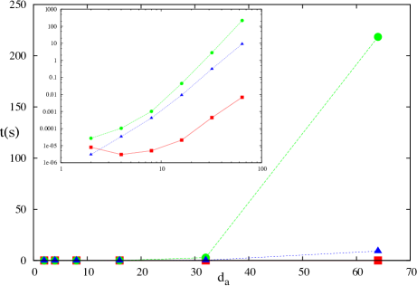
Figure 1: (color online) Time taken to compute the partial trace using Eqs. (1), (23), and (31) (from up down) as a function of system $a$ dimension. In the inset is shown the log-log plot of the same data. We set $d_{b}=d_{a}$ and used the maximally mixed global state in all cases. The calculations were performed using the GNU Fortran Compiler version 5.0.0 in a MacBook Air Processor 1.3 GHz Intel Core i5, with a 4 GB 1600 MHz DDR3 Memory. If, for $d_{a},d_{b}\gg 1$ and $d_{a}=d_{b}$, we have $t\propto d_{a}^{p}d_{b}^{q}$, then $\log t\propto(p+q)\log d_{a}$. So, the increasing rate of $\log t$ with the number of quantum bits Nielsen=000026Chuang constituting $a$ in the optimized implementation of the partial trace is one fourth of that for the direct calculation.

IV Partial trace for multi-partitions

Let us consider a multipartite system $\mathcal{H}=\bigotimes_{s}\mathcal{H}_{s}$ and a linear operator $O\in\mathcal{L}(\mathcal{H})$. For two arbitrary sub-systems $s^{\prime}$ and $s^{\prime\prime}$, with $s^{\prime\prime}>s^{\prime}$, and bases $|s_{j}^{\prime}\rangle\in\mathcal{H}_{s^{\prime}}$ and $|s_{j}^{\prime\prime}\rangle\in\mathcal{H}_{s^{\prime\prime}}$, one can verify that

$$(\mathbb{I}_{s^{\prime}}\otimes\mathbb{I}_{(s^{\prime}+1)\cdots(s^{\prime\prime}-1)}\otimes|s_{k}^{\prime\prime}\rangle)(|s_{j}^{\prime}\rangle\otimes\mathbb{I}_{(s^{\prime}+1)\cdots(s^{\prime\prime}-1)})=|s_{j}^{\prime}\rangle\otimes\mathbb{I}_{(s^{\prime}+1)\cdots(s^{\prime\prime}-1)}\otimes|s_{k}^{\prime\prime}\rangle.$$ (33)

We then use this relation to see that the equality

$$\mathrm{Tr}_{s^{\prime}s^{\prime\prime}}(O)=\mathrm{Tr}_{s^{\prime}}(\mathrm{Tr}_{s^{\prime\prime}}(O))$$ (34)

holds for all $s^{\prime}$ and $s^{\prime\prime}$. Therefore the partial trace taken over any set of sub-systems of $\mathcal{H}$ can be implemented sequentially via partial tracing over single partitions; and we can do that using the following two main procedures. In one of these procedures we split $\mathcal{H}$ in two parts $\mathcal{H}_{a}\otimes\mathcal{H}_{b}$ and trace out $a$ or $b$. And in the other one we divide $\mathcal{H}$ in three parties $\mathcal{H}_{a}\otimes\mathcal{H}_{b}\otimes\mathcal{H}_{c}$ and trace over the inner party $b$. As the first procedure was addressed in the previous section, we shall regard the details of the last one in this section.

Let $O\in\mathcal{L}(\mathcal{H}_{a}\otimes\mathcal{H}_{b}\otimes\mathcal{H}_{c})$ and let us consider the partial trace

$$O^{ac}=\mathrm{Tr}_{b}(O)=\sum_{j=1}^{d_{b}}(\mathbb{I}_{a}\otimes\langle b_{j}|\otimes\mathbb{I}_{c})O(\mathbb{I}_{a}\otimes|b_{j}\rangle\otimes\mathbb{I}_{c}).$$ (35)

In a direct implementation of this equation, $d_{a}^{2}d_{b}^{2}d_{c}^{2}(d_{a}d_{c}(d_{b}+1)+2)$ mops and $d_{a}^{2}d_{b}d_{c}^{2}(d_{b}+1)(d_{a}d_{b}d_{c}-1)$ sops would be used. For $d_{b}\gg 1$,

$$\mbox{mops}=\mbox{sops}\approx d_{a}^{3}d_{b}^{3}d_{c}^{3}.$$ (36)

With the aim of reaching an optimized computation of the partial trace, we start considering

$$O^{ac} = \sum_{j,m=1}^{d_{a}}\sum_{k,n=1}^{d_{b}}\sum_{l,o=1}^{d_{c}}(\langle j|\otimes\langle k|\otimes\langle l|)O(|m\rangle\otimes|n\rangle\otimes|o\rangle)|j\rangle\langle m|\otimes\mathrm{Tr}_{b}(|k\rangle\langle n|)\otimes|l\rangle\langle o|$$ (37)

$$= \sum_{j,m=1}^{d_{a}}\sum_{l,o=1}^{d_{c}}\left(\sum_{k=1}^{d_{b}}(\langle j|\otimes\langle k|\otimes\langle l|)O(|m\rangle\otimes|k\rangle\otimes|o\rangle)\right)|j\rangle\langle m|\otimes|l\rangle\langle o|$$ (38)

$$= \sum_{j,m=1}^{d_{a}}\sum_{l,o=1}^{d_{c}}(\langle j|\otimes\langle l|)O^{ac}(|m\rangle\otimes|o\rangle)|j\rangle\langle m|\otimes|l\rangle\langle o|.$$ (39)

In this article, if not stated otherwise, we assume that the matrix representation of the considered operators in the corresponding (global) computational basis is given. Next we notice e.g. that only the element $\alpha:=(m-1)d_{b}d_{c}+(n-1)d_{c}+o$ of $|m\rangle\otimes|n\rangle\otimes|o\rangle$ is non-null; thus $O|m\rangle\otimes|n\rangle\otimes|o\rangle$ is equal to the $\alpha$-th column vector of $O$. Thus, Eqs. (38) and (39) and these results can be used to write the following relation between matrix elements (in the corresponding global computational basis):

$$O_{(j-1)d_{c}+l,(m-1)d_{c}+o}^{ac}=\sum_{k=1}^{d_{b}}O_{(j-1)d_{b}d_{c}+(k-1)d_{c}+l,(m-1)d_{b}d_{c}+(k-1)d_{c}+o}.$$ (40)

In terms of ops, in this implementation we shall utilize $\mbox{mops}=0$ and $\mbox{sops}=d_{a}^{2}d_{c}^{2}(d_{b}-1)$, which for $d_{b}\gg 1$ is

$$\mbox{mops}=0\mbox{ and }\mbox{sops}\approx d_{a}^{2}d_{b}d_{c}^{2}.$$ (41)

As in the case of bipartite systems, here also we can utilize the hermiticity of the reduced matrix to diminish the number of basic operations by $2^{-1}d_{a}d_{c}(d_{a}d_{c}-1)(d_{b}-1)$ sops.

Fortran code to perform all numerical calculations associated with this article, and several others, can be accessed in https://github.com/jonasmaziero/LibForQ.git. In particular, we provide the subroutine, partial_trace(rho, d, di, nss, ssys, dr, rhor), which returns the reduced matrix rhor once provided dr (its dimension), rho (the matrix representation in the computational basis of the regarded linear operator in $\mathcal{H}_{1}\otimes\mathcal{H}_{2}\otimes\cdots\otimes\mathcal{H}_{n}$), d (the dimension of rho), nss$=n$ (the number of sub-systems), di (a $n$-dimensional integer vector whose components specify the dimensions of the sub-systems), and ssys (a $n$-dimensional integer vector whose null components specify the sub-systems to be traced over; the other components must be made equal to one). In the Hermitian case, just change the subroutine’s name to partial_trace_he.

Let’s exemplify the application of what was discussed in this section by considering the thermal ground state Nielsen_EntPT , $\rho=\exp(-\beta H)/\mathrm{Tr}(\exp(-\beta H))$ with $\beta\rightarrow\infty$, of a line of qubits with Ising interaction between nearest-neighbors: $H=-\frac{J}{2}\sum_{j=1}^{n-1}\sigma_{j}^{z}\sigma_{j+1}^{z}-h\sum_{j=1}^{n}\sigma_{j}^{x},$ where $\sigma_{j}^{x(z)}$ are the Pauli operators in the state space of the $j$-th spin, $h$ is the so called transverse magnetic field, and we set the exchange interaction strength to unit ($J=1$). Here we want to compute the nonlocal quantum coherence Maziero_QCS of the edge spins: $C_{nl}(\rho_{1n})=C(\rho_{1n})-[C(\rho_{1})+C(\rho_{n})],$ where the $l_{1}$-norm quantum coherence is given by Plenio_QQC : $C(\rho)=\sum_{j\neq k}\langle j|\rho|k\rangle,$ with $|j\rangle$ being the standard-computational basis in the regarded Hilbert space. When performing this kind of calculation, we shall need the reduced states: $\rho_{1n}=\mathrm{Tr}_{2\cdots(n-1)}(\rho_{12\cdots(n-1)n})\mbox{, }\rho_{1}=\mathrm{Tr}_{n}(\rho_{1n})\mbox{, and }\rho_{n}=\mathrm{Tr}_{1}(\rho_{1n}).$ The results for the quantum coherence and a comparison between the time taken by the optimized and direct implementations of the partial trace function are shown in Fig. 2.

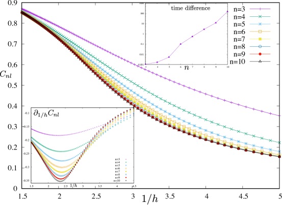
Figure 2: (color online) Non-local quantum coherence (NLQC) of the edge qubits of an Ising chain with $n$ spins as a function of the reciprocal of the transverse magnetic field. In the bottom inset is shown the first derivative of the NLQC, whose minimum is seem to go slowly towards the point of quantum phase transition ($h=1/2$). In the upper inset is shown, in logarithmic scale, the difference between the time taken, to do the calculations for a fixed value of $n$, by the direct and optimized implementations of the partial trace function. We notice thus a exponential increase of this time difference with $n$.

V “Partial traces” via Bloch’s parametrization

As the most frequent application of the partial trace function is to compute reduced density matrices (also called partial states or quantum marginals), let us consider yet another approach we may apply to perform that task and analyze its computational complexity. From the defining properties of a density matrix (positiveness $\rho\geq 0$ and unit trace $\mathrm{Tr}(\rho)=1$), follows that it can be written in terms of $\mathbb{I}_{b}$ and of the orthonormal-traceless-hermitian generators $\Gamma_{j}$ of the special unitary group, as shown below. For a bipartite system $\mathcal{H}_{a}\otimes\mathcal{H}_{b}$, the reduced state of sub-system $b$ can be written as Petruccione_rrho ; Bertlmann :

$$\rho^{b}=\frac{\mathbb{I}_{b}}{d_{b}}+\sum_{j=1}^{d_{b}^{2}-1}\frac{\gamma_{j}}{2}\Gamma_{j},$$ (42)

where $\mathrm{Tr}_{b}(\Gamma_{j}^{\dagger}\Gamma_{k})=2\delta_{jk}$ and $\gamma_{j}=\mathrm{Tr}_{b}(\Gamma_{j}\rho^{b})$. If the density matrix $\rho$ of the whole system is known, and we want to compute $\rho^{b}$, then

$$\gamma_{j}=\mathrm{Tr}_{b}(\Gamma_{j}\rho^{b})=\mathrm{Tr}_{ab}(\mathbb{I}_{a}\otimes\Gamma_{j}\rho)=\sum_{k=1}^{d_{a}d_{b}}(\mathbb{I}_{a}\otimes\Gamma_{j}\rho)_{k,k}$$ (43)

will yield the $d_{b}^{2}-1$ real components of the Bloch vector $\vec{\gamma}=[\gamma_{1}\mbox{ }\gamma_{2}\mbox{ }\cdots\mbox{ }\gamma_{d_{b}^{2}-1}]^{t}$.

V.1 Direct implementation

Let us start by the most straightforward, unoptimized, implementation of the partial trace via Bloch parametrization. Counting the basic operations need to compute each $\gamma_{j}$, we note that for the tensor product $\mathbb{I}_{a}\otimes\Gamma_{j}$, $\mbox{mops}=d_{a}^{2}d_{b}^{2}$, for the matrix multiplication $(\mathbb{I}_{a}\otimes\Gamma_{j})\rho$, $\mbox{mops}=d_{a}^{3}d_{b}^{3}$ and $\mbox{sops}=d_{a}^{2}d_{b}^{2}(d_{a}d_{b}-1)$, and for the trace, $\mbox{sops}=d_{a}d_{b}-1$. Then, for the $d_{b}^{2}-1$ components $\gamma_{j}$ we shall need $\mbox{mops}=(d_{b}^{2}-1)d_{a}^{2}d_{b}^{2}(d_{a}d_{b}+1)$ and $\mbox{sops}=(d_{b}^{2}-1)(d_{a}^{2}d_{b}^{2}+1)(d_{a}d_{b}-1)$. After knowing $\vec{\gamma}$, $d_{b}^{4}$ mops and $d_{b}^{2}(d_{b}^{2}-2)+d_{b}$ sops are required to compute $\rho^{b}$. Thus, on total we have to do $\mbox{mops}=d_{b}^{2}(d_{b}^{2}+d_{a}^{2}(d_{b}^{2}-1)(d_{a}d_{b}+1))$ and $\mbox{sops}=(d_{b}^{2}-1)(d_{a}^{2}d_{b}^{2}+1)(d_{a}d_{b}-1)+d_{b}^{2}(d_{b}^{2}-2)+d_{b}$, which for $d_{b}\gg 1$ become

$$\mbox{mops}=\mbox{sops}\approx d_{a}^{3}d_{b}^{5}.$$ (44)

V.2 (Not) Using the zeros of $\mathbb{I}_{a}$

Now let’s use the zeros of $\mathbb{I}_{a}$ to diminish the number of ops needed to obtain $\gamma_{j}$. We begin by writing

$$(\mathbb{I}_{a}\otimes\Gamma_{j})\rho=\begin{bmatrix}\Gamma_{j}&0_{d_{b}\mathrm{x}d_{b}}&\cdots&0_{d_{b}\mathrm{x}d_{b}}\\ 0_{d_{b}\mathrm{x}d_{b}}&\Gamma_{j}&\cdots&0_{d_{b}\mathrm{x}d_{b}}\\ \vdots&\vdots&\ddots&\vdots\\ 0_{d_{b}\mathrm{x}d_{b}}&0_{d_{b}\mathrm{x}d_{b}}&\cdots&\Gamma_{j}\end{bmatrix}\begin{bmatrix}\rho^{(1)}&[?]&\cdots&[?]\\ {}[?]&\rho^{(2)}&\cdots&[?]\\ \vdots&\vdots&\ddots&\vdots\\ {}[?]&[?]&\cdots&\rho^{(d_{a})}\end{bmatrix}=\begin{bmatrix}\Gamma_{j}\rho^{(1)}&\Gamma_{j}[?]&\cdots&\Gamma_{j}[?]\\ \Gamma_{j}[?]&\Gamma_{j}\rho^{(2)}&\cdots&\Gamma_{j}[?]\\ \vdots&\vdots&\ddots&\vdots\\ \Gamma_{j}[?]&\Gamma_{j}[?]&\cdots&\Gamma_{j}\rho^{(d_{a})}\end{bmatrix},$$ (45)

where $0_{d_{b}\mathrm{x}d_{b}}$ is the $d_{b}\mathrm{x}d_{b}$ null matrix and $[?]$ is used to denote those $d_{b}\mathrm{x}d_{b}$ sub-blocks of $\rho$ that we do not need when computing $\gamma_{j}$. From the last equation we see that

$$\gamma_{j} = \sum_{\beta=1}^{d_{a}}\mathrm{Tr}(\Gamma_{j}\rho^{(\beta)})=\sum_{\beta=1}^{d_{a}}\sum_{\alpha=1}^{d_{b}}(\Gamma_{j}\rho^{(\beta)})_{\alpha,\alpha}=\sum_{\beta=1}^{d_{a}}\sum_{\alpha=1}^{d_{b}}\sum_{k=1}^{d_{b}}(\Gamma_{j})_{\alpha,k}\rho_{k,\alpha}^{(\beta)}$$ (46)

$$= \sum_{\alpha=1}^{d_{b}}\sum_{k=1}^{d_{b}}(\Gamma_{j})_{\alpha,k}\sum_{\beta=1}^{d_{a}}\rho_{(\beta-1)d_{b}+k,(\beta-1)d_{b}+\alpha},$$ (47)

which is valid for any choice of the generators $\Gamma_{j}$. If computed as shown in the last equation, each $\gamma_{j}$ requires $\mbox{sops}=d_{b}^{2}(d_{a}-1)$ and $\mbox{mops}=d_{b}^{2}$, and we need to compute $d_{b}^{2}-1$ of them. Thus, when accounted for also the ops necessary to compute Eq. (42) given $\vec{\gamma}$, we arrive at a total of $2d_{b}^{2}(d_{b}^{2}-1)$ mops and $d_{b}^{2}((d_{b}^{2}-1)d_{a}-1)+d_{b}$ sops needed to compute $\rho^{b}$. For $d_{b}\gg 1$:

$$\mbox{mops}\approx 2d_{b}^{4}\mbox{ and }\mbox{sops}\approx d_{a}d_{b}^{4}.$$ (48)

V.3 (Not) Using the zeros of $\Gamma_{j}$ (and of $\mathbb{I}_{b}$)

These numbers can be reduced even more if we use the zeros of the generators $\Gamma_{j}$. To do that, a particular basis $\Gamma_{j}$ has to be chosen, and we shall pick here the generalized Gell Mann’s matrices Bertlmann :

$$\Gamma_{j}^{(1)}=\sqrt{\frac{2}{j(j+1)}}\left(\sum_{k=1}^{j}|k\rangle\langle k|-j|j+1\rangle\langle j+1|\right),\mbox{ for }j=1,\cdots,d_{b}-1,$$ (49)

$$\Gamma_{(k,l)}^{(2)}=|k\rangle\langle l|+|l\rangle\langle k|,\mbox{ for }1\leq k<l\leq d_{b},$$ (50)

$$\Gamma_{(k,l)}^{(3)}=-i(|k\rangle\langle l|-|l\rangle\langle k|),\mbox{ for }1\leq k<l\leq d_{b}.$$ (51)

From Eq. (47), when computing the components of the Bloch vector, we see that for the generators corresponding to the diagonal group in Eq. (49):

$$\gamma_{j}^{(1)}=\sqrt{\frac{2}{j(j+1)}}\sum_{\alpha=1}^{j+1}(-j)^{\delta_{\alpha,j+1}}\sum_{\beta=1}^{d_{a}}\rho_{(\beta-1)d_{b}+\alpha,(\beta-1)d_{b}+\alpha}.$$ (52)

Then $6(d_{b}-1)$ mops and $1+(d_{a}-1)(\sum_{j=1}^{d_{b}}j)=1+(d_{a}-1)2^{-1}d_{b}(d_{b}+1)$ sops are used for this first group. Related to the generators belonging to the symmetric and anti-symmetric groups in Eqs. (50) and (51), respectively, from Eq. (47) we get

$$\gamma_{(k,l)}^{(2)} = \sum_{\beta=1}^{d_{a}}\left(\rho_{(\beta-1)d_{b}+l,(\beta-1)d_{b}+k}+\rho_{(\beta-1)d_{b}+k,(\beta-1)d_{b}+l}\right)=2\sum_{\beta=1}^{d_{a}}\mathrm{Re}(\rho_{(\beta-1)d_{b}+l,(\beta-1)d_{b}+k}),$$ (53)

$$\gamma_{(k,l)}^{(3)} = -i\sum_{\beta=1}^{d_{a}}\left(\rho_{(\beta-1)d_{b}+l,(\beta-1)d_{b}+k}-\rho_{(\beta-1)d_{b}+k,(\beta-1)d_{b}+l}\right)=2\sum_{\beta=1}^{d_{a}}\mathrm{Im}(\rho_{(\beta-1)d_{b}+l,(\beta-1)d_{b}+k}).$$ (54)

These two groups, formed by $d_{b}(d_{b}-1)/2$ elements each, entail in $\mbox{mops}=2$ and $\mbox{sops}=2(d_{a}-1)$; but, as we will see below, we do not need them to compute the reduced state $\rho^{b}$.

In the sequence, we shall rewrite the partial state splitting its diagonal $\Delta$ and non-diagonal $\Theta$ parts, i.e.,

$$\rho^{b}=\Delta+\Theta.$$ (55)

We will look first at the diagonal elements of $\rho^{b}$:

$$\Delta = \frac{\mathbb{I}_{b}}{d_{b}}+\sum_{j=1}^{d_{b}-1}\frac{\gamma_{j}^{(1)}}{2}\Gamma_{j}^{(1)}=\frac{\sum_{k=1}^{d_{b}}|k\rangle\langle k|}{d_{b}}+\sum_{j=1}^{d_{b}-1}\frac{\gamma_{j}^{(1)}}{2}\sqrt{\frac{2}{j(j+1)}}\left(\sum_{k=1}^{j}|k\rangle\langle k|-j|j+1\rangle\langle j+1|\right).$$ (56)

If, for $j=1,\cdots,d_{b}-1$, we define the function $\xi_{j}=\gamma_{j}^{(1)}/\sqrt{2(j(j+1))}$ and set $\xi_{0}=d_{b}^{-1}$ and $q=d_{b}$, then

$$\Delta = \mathrm{diag}(\xi_{0},\xi_{0},\xi_{0},\xi_{0},\xi_{0},\cdots,\xi_{0})+\mathrm{diag}(\xi_{1},-\xi_{1},0,0,0,\cdots,0)+\mathrm{diag}(\xi_{2},\xi_{2},-2\xi_{2},0,0,\cdots,0)$$ (59)

$$+\mathrm{diag}(\xi_{3},\xi_{3},\xi_{3},-3\xi_{3},0,\cdots,0)+\cdots+\mathrm{diag}(\xi_{q-3},\cdots,\xi_{q-3},-(q-3)\xi_{q-3},0,0)$$

$$+\mathrm{diag}(\xi_{q-2},\xi_{q-2},\cdots,\xi_{q-2},-(q-2)\xi_{q-2},0)+\mathrm{diag}(\xi_{q-1},\xi_{q-1},\xi_{q-1},\xi_{q-1},\cdots,\xi_{q-1},-(q-1)\xi_{q-1}).$$

After some analysis, we see that

$$\Delta_{1,1} =\sum_{k=0}^{d_{b}-1}\xi_{k} \mbox{ and }\Delta_{j,j}=\Delta_{j-1,j-1}+(j-2)\xi_{j-2}-j\xi_{j-1}\mbox{ for }j=2,\cdots,d_{b}.$$ (60)

If we know the $\gamma_{j}^{(1)}$’s, for the $\xi_{j}$’s $\mbox{mops}=4(d_{b}-1)+1$ and $\mbox{sops}=d_{b}-1$ and for the $\Delta_{j,j}$’s $2\mbox{mops}=\mbox{sops}=4(d_{b}-1)$. Then for $\Delta$ we shall need $6(d_{b}-1)+1$ mops and $5(d_{b}-1)$ sops.

Let us now consider the off-diagonal elements of $\rho^{b}$:

$$\Theta = \sum_{1\leq k<l\leq d_{b}}\frac{1}{2}\left(\gamma_{(k,l)}^{(2)}\Gamma_{(k,l)}^{(2)}+\gamma_{(k,l)}^{(3)}\Gamma_{(k,l)}^{(3)}\right)=\sum_{1\leq k<l\leq d_{b}}\frac{1}{2}\left((\gamma_{(k,l)}^{(2)}-i\gamma_{(k,l)}^{(3)})|k\rangle\langle l|+(\gamma_{(k,l)}^{(2)}+i\gamma_{(k,l)}^{(3)})|l\rangle\langle k|\right).$$ (61)

Using Eqs. (53) and (54) we arrive at

$$\Theta_{l,k}=\sum_{\beta=1}^{d_{a}}\rho_{(\beta-1)d_{b}+l,(\beta-1)d_{b}+k}.$$

Then, as $\Theta_{k,l}=\Theta_{l,k}^{*}$, we shall need $\mbox{sops}=2^{-1}d_{b}(d_{b}-1)(d_{a}-1)$ to calculate $\Theta$. So, after knowing $\vec{\gamma}$, $6(d_{b}-1)+1$ mops and $(d_{b}-1)(2^{-1}d_{b}(d_{a}-1)+5)$ sops are used to compute $\rho^{b}$. Therefore, counting the ops need to compute the $\gamma_{j}^{(1)}$’s, on total $\mbox{mops}=12(d_{b}-1)+1$ and $\mbox{sops}=d_{b}^{2}(d_{a}-1)+5(d_{b}-1)+1$ shall be used to get $\rho^{b}$ via Bloch parametrization. And for $d_{a},d_{b}\gg 1$

$$\mbox{mops}\approx 12d_{b}\mbox{ and }\mbox{sops}\approx d_{a}d_{b}^{2}.$$ (62)

As the “worst case” complexity for the multiplication is equal to the square of the complexity for the addition, we see that this number of operations is comparable with the optimized one obtained in Sec. III.3, for $d_{a},d_{b}\gg 1$. Here is another, more dramatic example of the reduction in the number of elementary operations needed to compute the partial trace ($\mathcal{O}(d_{a}^{6}d_{b}^{10})\rightarrow\mathcal{O}(d_{a}d_{b}^{2})$), which is obtained simply by performing some analytical developments. We also provide the Fortran code to compute partial states of bipartite systems via Bloch’s parametrization using this last procedure, i.e., with generalized Gell Mann’s matrices.

VI Concluding remarks

In this article, a thorough discussion about the partial trace function was made. We gave special attention to its numerical implementation. It is a good programming practice trying to avoid making the computer perform calculations which make no difference to the final result. We showed here that by following this truism we can decrease considerably the number of elementary operations needed to compute the partial trace, or reduced density matrix, which is an extremely important and common procedure in the quantum mechanics of composite (and open) systems. We provided and described Fortran code for computing the partial trace over any set of parties of a discrete multipartite system. At last, we analyzed the calculation of partial states via the Bloch’s parametrization with generalized Gell Mann’s matrices. We believe this text will be of pedagogical and practical value for the physics and quantum information science communities. As the partial trace function is highly adaptable for parallel calculations, we think this is a natural theme for future investigations. Extending our approach to continuous variable systems is an interesting research topic. It would also be fruitful producing translations of our code to other open source programming languages such as e.g. Maxima and Octave, as was already done for Python.