We study the global structure of some exact scalar hairy dynamical black holes which were constructed in Einstein gravity either minimally or non-minimally coupled to a scalar field. We find that both the apparent horizon and the local event horizon (measured in luminosity coordinate) monotonically increase with the advanced time as well as the Vaidya mass. At late advanced times, the apparent horizon approaches the event horizon and gradually becomes future outer. Correspondingly, the space-time arrives at stationary black hole states with the relaxation time inversely proportional to the $1/(n-1)$ power of the final black hole mass, where $n$ is the space-time dimension. These results strongly support the solutions describing the formation of black holes with scalar hair. We also obtain new charged dynamical solutions in the non-minimal theory by introducing an Maxwell field which is non-minimally coupled to the scalar. The presence of the electric charge strongly modifies the dynamical evolution of the space-time.

Emails: fanzhy@pku.edu.cn, bchen01@pku.edu.cn,   mrhonglu@gmail.com

1 Introduction

The no-hair theorems in General Relativity exclude the existence of hairy black holes in asymptotically flat space-times for a variety of theories. However, it turns out that the no-hair theorems are easily evaded. People have found many counter examples in recent years. For instance, many scalar hairy black holes that are asymptotic to Minkowski space-times have been analytically constructed in Einstein gravity minimally coupled to a scalar field [1, 2, 3, 4, 5]. Rotating black holes with scalar hair were also numerically studied in [6]. Black holes with vector hair [7] and with Yang-Mills hair [8, 9, 10, 11, 12] have also been found in literature. By numerical analysis, it was established that non-Schwarzschild black holes do exist in higher derivative gravity in four dimensions [13, 14].

For asymptotical (anti-)de Sitter space-times, the condition for the no-hair theorems was much relaxed. There are large classes of scalar hairy black holes having been constructed in Einstein gravity either minimally or non-minimally coupled to a scalar field [2, 3, 4, 5, 15, 16, 17, 18, 19, 20]. More interestingly, some of these theories even admit exact dynamical black holes solutions with scalar hair [20, 21, 22, 23, 24, 25, 26]. The solutions provide explicit and analytical examples for the formation of scalar hairy black holes. In particular, one class of solutions analytically shows how the linearly stable AdS vacua undergoes non-linear instability and spontaneously evolves into stationary black holes states [20, 26]. The solutions that are asymptotic to AdS space-times also have potential applications in the AdS/CFT correspondence.

The purpose of current paper is to gain an even deeper understanding of the scalar hairy dynamical solutions which were found in certain minimally and non-minimally coupled Einstein-scalar gravity by studying their global properties. We focus on discussing the dynamical evolution of the apparent horizon which was studied as a function of the advanced time. We find that the apparent horizon (measured in luminosity coordinate) grows monotonically with the advanced time and approaches the event horizon at the future infinity. At late times of the evolution, the apparent horizon smoothly evolves and becomes future outer gradually. In addition, it is also instructive to study the dynamical evolution of the event horizon for our solutions. Unfortunately, the event horizon is in general hard to be established in dynamical space-times, though it is globally well defined. Instead, we adopt an effective notion “local event horizon”. We find that it covers the apparent horizon in the whole dynamical process and also approaches the event horizon at the future infinity. These results provide strong evidence to support the dynamical solutions describing black holes formation.

Moreover, we generalize the non-minimally coupled Einstein-scalar gravity by introducing an additional Maxwell field which is non-minimally coupled to the scalar. We obtain new charged dynamical solutions for proper gauge coupling functions. The dynamical evolution of the space-time turns out to be strongly dependent on the electric charges. The global property of the charged solutions differs significantly from the pure neutral solutions.

This paper is organized as follows. In section 2, we present some preliminaries for studying the global properties of dynamical solutions. In section 3, we study two explicit examples: the dynamical solutions that are constructed in certain minimally and non-minimally coupled Einstein-scalar gravity. In section 4, we obtain more charged dynamical solutions in the non-minimal theory and discuss their global properties. We conclude this paper in section 5.

2 Global properties of dynamical solutions

In this section, we give the preliminaries for studying the global structure of dynamical solutions of the type

$$ds^{2}=-Hdu^{2}+2hdudr+\rho^{2}d\Omega_{n-2}^{2}\,,$$ (1)

where $H,h$ and $\rho$ are all functions of the Eddington-Finkelestein-type coordinates $r$ and $u$ and $d\Omega_{n-2}$ is the $(n-2)$ dimensional space with spherical/torus/hyperbolic symmetries.

2.1 Local event horizon

The event horizon of a static black hole can be easily established corresponding to a null Killing vector with non-negative surface gravity. The situation for a dynamical solution is much more subtle. The location of the event horizon cannot be solved in general even for an exact black hole solution. We shall adopt a local definition for the event horizon, which can be found in many standard textbooks and some early literature such as [27, 28]. We call it “local event horizon”. It is defined by a null hypersurface which preserves the isometry of the space-time. That is, if the null hypersurface is parameterized by:

$$F(r\,,u)=0\,,$$ (2)

with $r=r(u)$, it satisfies

$$g^{\mu\nu}{\frac{\partial F}{\partial x^{\mu}}}{\frac{\partial F}{\partial x^{\nu}}}=0\,.$$ (3)

This gives

$$H{\frac{\partial F}{\partial r}}+2h{\frac{\partial F}{\partial u}}=0\,.$$ (4)

On the other hand, we have

$$0\equiv{\frac{dF}{du}}={\frac{\partial F}{\partial u}}+{\frac{\partial F}{\partial r}}{\frac{dr}{du}}\,.$$ (5)

Combining these two equations, we find

$${\frac{dr}{du}}={\frac{H}{2h}}\,.$$ (6)

It follows that the local event horizon coincides with the “true” event horizon in the stationary limit. However, we should point out that it is not clear what the precise relation is between the local event horizon and the event horizon in dynamical space-times. In this paper, we simply take it to be an effective conception for describing black holes formation. Indeed, we find that it enjoys some reasonable aspects for our solutions. For example, the local event horizon always encloses the apparent horizon in the dynamical process and approaches the event horizon at the future infinity.

2.2 The apparent horizon

For the dynamical solutions with planar topology describing gravitational collapse, a sufficient condition is the apparent horizon should be future outer at late advanced times [29]. We shall first give a general discussion on this topic. The tangent vector of radial null geodesic congruences can be given by:

$$k_{\epsilon}^{a}\equiv({\textstyle{\frac{\scriptstyle\partial}{\scriptstyle\partial\xi_{\epsilon}}}})^{a}=\epsilon\Big{(}({\textstyle{\frac{\scriptstyle\partial}{\scriptstyle\partial u}}})^{a}+{\textstyle{\frac{\scriptstyle H}{\scriptstyle 2h}}}({\textstyle{\frac{\scriptstyle\partial}{\scriptstyle\partial r}}})^{a}\Big{)}\,,$$ (7)

where $\epsilon=-1$ for ingoing null geodesic congruences and $\epsilon=+1$ for outgoing null geodesic congruences respectively. It is straightforward to verify that $k_{\epsilon}^{a}$ is null and it satisfies the null geodesic equations of motions, namely

$$k_{\epsilon}^{b}\triangledown_{b}k_{\epsilon}^{a}=\lambda_{\epsilon}k_{\epsilon}^{a}\,,\qquad\lambda_{\epsilon}={\frac{\epsilon}{2h}}(2h_{u}+H_{r})\,,$$ (8)

where $H_{r}\equiv{\frac{\partial H}{\partial r}},\ h_{u}\equiv{\frac{\partial h}{\partial u}}$. Given the tangent vector, it is easy to calculate the expansion

$$\theta_{\epsilon}=g_{ab}\triangledown^{b}k_{\epsilon}^{a}-\lambda_{\epsilon}={\textstyle{\frac{\scriptstyle\epsilon(n-2)}{\scriptstyle 2}}}\Big{(}{\frac{H\rho_{r}}{h\rho}}+{\frac{2\rho_{u}}{\rho}}\Big{)}\,,$$ (9)

where $\rho_{r}\,,\rho_{u}$ denotes the derivatives of $\rho$ with respect to $r$ and $u$ respectively. The location of the apparent horizon is defined by $\theta_{\epsilon}=0$. In the luminosity coordinate $\rho\equiv r$, the expansion was simplified to be $\theta_{\epsilon}={\textstyle{\frac{\scriptstyle\epsilon(n-2)H}{\scriptstyle 2hr}}}$. It is immediately seen that the expansion of the ingoing null geodesic congruences $\theta_{-}$ is negative outside the apparent horizon($H(r,u)>0$), which implies that the apparent horizon is future. This is independent of the coordinate system and is valid for more general $\rho$ coordinate.

In order to show the apparent horizon is outer, we need compute the Lie derive of the expansion of the ingoing null geodesic congruences along the tangent vector of the outgoing null geodesic congruences

$$\mathcal{L}_{k_{+}}\theta_{-} = k_{+}^{b}\triangledown_{b}\theta_{-}=k_{+}^{r}{\frac{\partial\theta_{-}}{\partial r}}+k_{+}^{u}{\frac{\partial\theta_{-}}{\partial u}}$$

$$= {\frac{(n-2)}{4\rho^{2}h^{3}}}\Big{(}4h^{3}(\rho_{u}^{2}-\rho\rho_{uu})-2h^{2}\rho\rho_{r}H_{u}$$

$$+\big{(}4h(\rho_{r}\rho_{u}-\rho\rho_{ru})+\rho\rho_{r}(2h_{u}-H_{r})\big{)}hH$$

$$+\big{(}h\rho_{r}^{2}+\rho(h_{r}\rho_{r}-h\rho_{rr})\big{)}H^{2}\Big{)}\,.$$

If this is also negative outside the apparent horizon, the apparent horizon is called outer. This is valid for planar black holes. For the solutions considered in this paper, we will show that the apparent horizon approaches the event horizon and smoothly evolves into a future outer one at the late times of the evolution.

3 Explicit examples

3.1 The non-minimal example

The first example we consider is non-minimally coupled Einstein-scalar gravity in general $n$ dimensions [20]. The Lagrangian is given by:

$$\mathcal{L}_{n}=\sqrt{-g}\Big{(}\kappa_{0}R-{\textstyle{\frac{\scriptstyle 1}{\scriptstyle 2}}}\xi\phi^{2}R-{\textstyle{\frac{\scriptstyle 1}{\scriptstyle 2}}}(\partial\phi)^{2}-V(\phi)\Big{)}\,,$$ (11)

where $\kappa_{0}$ is the bared gravitational coupling constant and $\xi$ is a constant that characterizes the coupling strength between the scalar $\phi$ and the curvature. The covariant equations of motion are

$$E_{\mu\nu}\equiv\kappa_{0}G_{\mu\nu}-T_{\mu\nu}^{\rm(min)}-T_{\mu\nu}^{\rm(non)}\,,\qquad\Box\phi=\xi\phi\,R+{\frac{dV}{d\phi}}\,,$$ (12)

where $G_{\mu\nu}=R_{\mu\nu}-{\frac{1}{2}}Rg_{\mu\nu}$ is the Einstein tensor and

$$T_{\mu\nu}^{\rm(min)} = {\textstyle{\frac{\scriptstyle 1}{\scriptstyle 2}}}\partial_{\mu}\phi\partial_{\nu}\phi-{\textstyle{\frac{\scriptstyle 1}{\scriptstyle 2}}}g_{\mu\nu}\Big{(}{\textstyle{\frac{\scriptstyle 1}{\scriptstyle 2}}}(\partial\phi)^{2}+V(\phi)\Big{)}\,,$$

$$T_{\mu\nu}^{\rm(non)} = {\textstyle{\frac{\scriptstyle 1}{\scriptstyle 2}}}\xi(\phi^{2}G_{\mu\nu}+g_{\mu\nu}\square\phi^{2}-\nabla_{\mu}\nabla_{\nu}\phi^{2})\,.$$ (13)

Without loss of generality, we let

$$\kappa_{0}={\frac{\xi}{2}}\,,$$ (14)

in this subsection. The effective gravitational coupling constant depends on $\phi$, given by

$$\kappa(\phi)=\kappa_{0}-{\textstyle{\frac{\scriptstyle 1}{\scriptstyle 2}}}\xi\phi^{2}={\textstyle{\frac{\scriptstyle 1}{\scriptstyle 2}}}\xi(1-\phi^{2})\,.$$ (15)

We shall require $\phi<1$ to cancel ghost-like graviton modes. For generic $\xi$, there are large classes of static hairy planar black holes which were reported in [20]. In particular, When $\xi$ takes the value

$$\xi=\frac{n-2}{4(n-1)}\,,$$ (16)

the non-minimal theory admits exact dynamic solutions with the potential given by

$$V=-{\textstyle{\frac{\scriptstyle 1}{\scriptstyle 8}}}(n-2)^{2}\Big{(}g^{2}+\alpha\phi^{{\frac{2(n-1)}{n-2}}}\big{(}{\textstyle{\frac{\scriptstyle 1}{\scriptstyle 1-\phi^{2}}}}-{}_{2}F_{1}[1,{\textstyle{\frac{\scriptstyle n-1}{\scriptstyle n-2}}};{\textstyle{\frac{\scriptstyle 2n-3}{\scriptstyle n-2}}};\phi^{2}]\big{)}\Big{)}\,.$$ (17)

The scalar potential has a stationary point $\phi=0$ and its small $\phi$ expansion is given by

$$V=-{\textstyle{\frac{\scriptstyle 1}{\scriptstyle 8}}}(n-2)^{2}g^{2}-{\frac{(n-2)^{3}\alpha}{8(2n-3)}}\phi^{4+{\frac{2}{n-2}}}-{\frac{(n-2)^{3}\alpha}{4(3n-5)}}\phi^{6+{\frac{2}{n-2}}}+\cdots\,.$$ (18)

It follows that the scalar has vanishing mass square, which is above the Breitenlohner-Freedman (BF) bound because $m_{\mathrm{BF}}^{2}=-{\textstyle{\frac{\scriptstyle 1}{\scriptstyle 4}}}g^{2}$ for the non-minimal coupling (16). This implies that the AdS vacua is linearly stable against perturbation.

In Eddington-Finkelstein-like coordinates, our dynamical solutions can be cast into the form of

$$ds^{2} = -fdu^{2}+2dudr+r^{2}dx^{i}dx^{i}\,,\qquad\phi=\Big{(}{\frac{a}{r}}\Big{)}^{{\frac{1}{2}}(n-2)}\,,$$ (19)

$$f = g^{2}r^{2}-{\frac{\alpha a^{n-1}}{r^{n-3}}}\,{}_{2}F_{1}[1,{\textstyle{\frac{\scriptstyle n-1}{\scriptstyle n-2}}};{\textstyle{\frac{\scriptstyle 2n-3}{\scriptstyle n-2}}},\big{(}{\textstyle{\frac{\scriptstyle a}{\scriptstyle r}}}\big{)}^{n-2}]\,,$$ (20)

where $a\equiv a(u)$ is the time dependent “scalar charge”. It satisfies a second order non-linear differential equation

$${\frac{\ddot{a}}{a^{2}}}-{\frac{2\dot{a}^{2}}{a^{3}}}+{\frac{\tilde{\alpha}\dot{a}}{a}}=0\,,\qquad\tilde{\alpha}={\textstyle{\frac{\scriptstyle 1}{\scriptstyle 2}}}(n-1)\alpha\,.$$ (21)

Here a dot denotes the derivative with respect to $u$. This equation can be integrated. The resulting first order equation is

$$\dot{a}+\tilde{\alpha}\,a^{2}\log\big{(}{\frac{a}{q}}\big{)}=0\,,$$ (22)

where $q$ is an integration constant. It is clear that both $a=0$ and $a=q$ are stationary points. The former corresponds to the pure AdS vacua whilst the latter corresponds to the stable black holes. The first order equation can be solved exactly in terms of an exponential integral function

$${\rm Ei}\big{(}\log({\textstyle{\frac{\scriptstyle q}{\scriptstyle a}}})\big{)}=-\tilde{\alpha}q\,u\,.$$ (23)

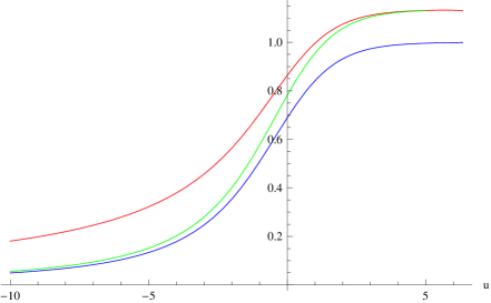
Figure 1: The plots for $a(u)$ (the blue line), the apparent horizon (the green line) and the local event horizon (the red line) for the $n=4$ dimension. At late advanced times $u\rightarrow\infty$, $a(u)$ approaches its equilibrium value $q$ and both horizons approach the event horizon at an exponential rate of $e^{-u/u_{0}}$, where $u_{0}=1/(\tilde{\alpha}q)$ is the characteristic relaxation time. Some constants $g^{2}\,,\tilde{\alpha}\,,q$ have been set to unity.

In Fig.1, we plot $a(u)$ as a function of the advanced time $u$ (the blue line). The advanced time coordinate $u$ runs over ($-\infty\,,+\infty$). Correspondingly, the space-time evolves from pure AdS vacua with $a=0$ at the past infinity to stable black holes states with $a=q$ at the future infinity. In addition, from the asymptotical behavior of the metric function $f$

$$f=g^{2}r^{2}-{\frac{\alpha a^{n-1}}{r^{n-3}}}+\cdots\,,$$ (24)

we can read off the effective Vaidya mass

$$M={\frac{(n-2)^{2}\alpha}{128(n-1)\pi}}a^{n-1}\,,$$ (25)

and deduce its first order derivative

$$\dot{M}={\frac{(n-1)(n-2)^{2}\alpha^{2}}{256\pi}}a^{n}\log\big{(}{\frac{q}{a}}\big{)}\,.$$ (26)

It follows that $\dot{M}$ is positive for $a<q$, implying that the Vaidya mass monotonically increases with the advanced time.

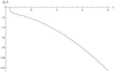
Figure 2: The plots for the Lie derivative $\mathcal{L}_{k_{+}}\theta_{-}$ for $n=4$ dimension. The left plot is given for static solutions and the Lie derivative is plotted as a function of $r$. In the right plot, the Lie derivative is plotted as a function of the advanced time $u$ for $r=r_{AH}$ (Green), $r=r_{EH}$ (Red) and $r=1.23$ (Blue), respectively. We have $r_{AH}<r_{EH}<1.23$. To have a nice presentation, we have properly scaled the Lie derivative on the apparent horizon as $\mathcal{L}_{k_{+}}\theta_{-}\rightarrow{\textstyle{\frac{\scriptstyle 1}{\scriptstyle 5}}}\mathcal{L}_{k_{+}}\theta_{-}$ and shifted it as $\mathcal{L}_{k_{+}}\theta_{-}\rightarrow\mathcal{L}_{k_{+}}\theta_{-}+0.715$ at $r=1.23$. Some constants $g^{2}\,,\tilde{\alpha}\,,q$ have been set to unity.

At the past infinity $u\rightarrow-\infty$, $a(u)$ behaves as $a\log a\sim-1/u$, indicating that the scalar only provides a weak source to perturb the space-time. However, the AdS vacuum is linearly stable against perturbation. It is some non-linear effects that pushes the space-time evolving into stationary black holes states. Hence, this solution provides an analytical example how the linearly stable AdS vacua undergoes non-linear instability and eventually settles down to stable black holes states.

In Fig.1, we also plot the apparent horizon (the green line) and the local event horizon (the red line) during the black holes formation. It is interesting to note that the apparent horizon is always inside the local event horizon in the whole dynamic process and both of them approach the event horizon at the large $u$ region. In fact, at the future infinity $u\rightarrow+\infty$, the space-time approaches the static limit exponentially fast. We find

$$a(u)=q\Big{(}1-c_{0}e^{-\tilde{\alpha}qu}+{\textstyle{\frac{\scriptstyle 3c_{0}^{2}}{\scriptstyle 2}}}e^{-2\tilde{\alpha}qu}+\cdots\Big{)}\,,$$

$$M(u)=M_{0}\Big{(}1-(n-1)c_{0}e^{-\tilde{\alpha}qu}+{\textstyle{\frac{\scriptstyle(n^{2}-1)c_{0}^{2}}{\scriptstyle 2}}}e^{-2\tilde{\alpha}qu}+\cdots\Big{)}\,.$$ (27)

Here $c_{0}$ is a positive integration constant which can be absorbed by constant shift of $u$ and $M_{0}$ is the static black hole mass, given by Eq.(25) with $a$ replaced by $q$. The apparent horizon and the local event horizon have analogous behaviors at late advanced times. Therefore, we can naturally define a characteristic relaxation time $u_{0}=1/(\tilde{\alpha}q)\sim 1/M_{0}^{{\frac{1}{n-1}}}$. It turns out that the relaxation time becomes shorter for a bigger black hole mass.

To end this subsection, we remark that our solutions have future outer apparent horizons. This is immediately seen from the behavior of the Lie derivative $\mathcal{L}_{k_{+}}\theta_{-}$ (see Fig.2). For the static solutions it vanishes on the apparent horizon and becomes negative outside the apparent horizon. In the dynamical process, the Lie derivative continuously evolves and approaches the static limit at late advanced times. These results imply that the apparent horizon is future outer and the dynamical solutions describe the physical process of black holes formation.

3.2 The minimal example

The second example we consider is the dynamical black holes which were found in certain minimal coupled Einstein-scalar gravity in four dimensions [21]. The Lagrangian is given by

$${\cal L} = \sqrt{-g}\Big{(}R-{\textstyle{\frac{\scriptstyle 1}{\scriptstyle 2}}}(\partial\phi)^{2}-V(\phi)\Big{)},$$ (28)

$$V = -2g^{2}(\cosh\phi+2)-2\alpha(2\phi+\phi\cosh\phi-3\sinh\phi)\,.$$ (29)

The scalar potential has a stationary point $\phi=0$ with small $\phi$ expansion

$$V=-6g^{2}-g^{2}\phi^{2}-{\textstyle{\frac{\scriptstyle 1}{\scriptstyle 12}}}g^{2}\phi^{4}-{\textstyle{\frac{\scriptstyle 1}{\scriptstyle 30}}}\alpha^{2}\phi^{5}+\cdots\,.$$ (30)

It follows that the scalar has a mass square $m^{2}=2g^{2}$ which is above the Breitenlohner-Freedman bound ($m_{BF}^{2}=-{\textstyle{\frac{\scriptstyle 9}{\scriptstyle 4}}}g^{2}$) in AdS space-time with $g^{2}>0$. In fact, the potential arises from $\mathcal{N}=4\,,D=4$ gauged supergravity for vanishing $\alpha$ and $g^{2}>0$ [30].

Using Eddington-Finekelstein-like coordinates, the dynamical solution reads

$$ds^{2} = -fdu^{2}+2dudr+r(r+a)d\Omega_{2,k}^{2}\,,\qquad\phi=\log{\Big{(}1+{\frac{a}{r}}\Big{)}}\,,$$ (31)

$$f = g^{2}r^{2}+k-{\textstyle{\frac{\scriptstyle 1}{\scriptstyle 2}}}\alpha a^{2}-\dot{a}+(g^{2}-\alpha)ar+\alpha r^{2}\Big{(}1+{\frac{a}{r}}\Big{)}\log\!\Big{(}1+{\frac{a}{r}}\Big{)}\,,$$ (32)

where $d\Omega_{2,k}$ is the $2$-space with constant curvature $k=0\,,\pm 1$. The time dependent “scalar charge” $a\equiv a(u)$ satisfies

$$\ddot{a}+\alpha a\dot{a}=0\,,$$ (33)

which can be solved immediately by

$$a=q\tanh{\Big{(}{\textstyle{\frac{\scriptstyle 1}{\scriptstyle 2}}}\alpha qu\Big{)}}\,.$$ (34)

It follows that $a=0$ at $u=0$. However, its first order derivative $\dot{a}={\textstyle{\frac{\scriptstyle 1}{\scriptstyle 2}}}\alpha q^{2}\mathrm{sech}{\Big{(}{\textstyle{\frac{\scriptstyle 1}{\scriptstyle 2}}}\alpha qu\Big{)}}$ is non-vanishing at this point. This results to subtle global structure around this point [21]. When $u$ goes to zero, the space-time turns out to be pure AdS except the singular point $R=0$, where $R$ is the luminosity coordinate defined by $R=\sqrt{r(r+a)}$. In fact, the existence of this singularity strongly depends on the path to $(0\,,0)$ point on the $(u\,,R)$ plane. We find that for some paths such as $R\propto u^{\delta}$ with $\delta\leq 1/3$, the singularity disappears. However, all these trajectories are space-like, indicating that this singularity is non-traversable.

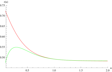
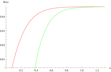
Figure 3: The dynamical evolution of apparent horizon (green) and local event horizon (red) for planar black holes $k=0$ in $r$ (left) and $R$ (right) coordinate, respectively. We have set $g^{2}\,,q$ to unity and $\alpha=2$.

In Fig.3, we plot the apparent horizon and the local event horizon as a function of the advanced time for planar black holes with $k=0$. We find that the apparent horizon is always enclosed by the local event horizon in the dynamical process. Note that in $r$ coordinate, both horizons become decreasing functions of the advanced time at late times. However, this does not mean the black objects are radiating energies. To clarify this point, we also plot the horizons in luminosity coordinate. We see that both horizons grow with the advanced time monotonically and approach the event horizon at the future infinity. For sphrical/hyperbolic black holes, we also find qualitatively similar features.

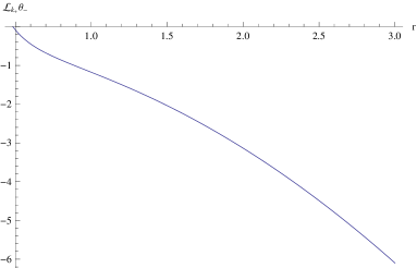
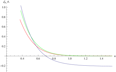
Figure 4: The plots of the Lie derivative $\mathcal{L}_{k_{+}}\theta_{-}$ for planar black holes. The left plot is presented for static solutions and the Lie derivative is plotted as a function of $r$. In the right plot, the Lie derivative is plotted as a function of the advanced time $u$ for $r=r_{AH}$ (Green), $r=r_{EH}$ (Red) and $r=0.53$ (Blue), respectively. We have set $g^{2}\,,q$ to unity and $\alpha=2$.

In addition, the Vaidya mass of the dynamical black holes is given by

$$M(u)={\textstyle{\frac{\scriptstyle 1}{\scriptstyle 2}}}M_{0}\tanh({\textstyle{\frac{\scriptstyle 1}{\scriptstyle 2}}}\alpha^{2}q\,u)\big{(}3-\tanh^{2}({\textstyle{\frac{\scriptstyle 1}{\scriptstyle 2}}}\alpha^{2}q\,u)\big{)}\geq 0\,,$$ (35)

which is a monotonically increasing function of the advanced time and approaches the final black hole mass $M_{0}={\textstyle{\frac{\scriptstyle 1}{\scriptstyle 12}}}\alpha q^{3}$. This is independent of the radial coordinates.

At the future infinity, the system exponentially reaches the static limit. We find

$$a=q\Big{(}1-2e^{-\alpha qu}+2e^{-2\alpha qu}+\cdots\Big{)}\,,\qquad M=M_{0}\Big{(}1-6e^{-2\alpha qu}+16e^{-3\alpha qu}+\cdots\Big{)}\,.$$ (36)

The characteristic relaxation time is given by $u_{0}=1/\big{(}\alpha q\big{)}$, which is inversely proportional to the cube root of the final black hole mass $u_{0}\sim 1/M_{0}^{1/3}$.

Finally, we plot the Lie derivative $\mathcal{L}_{k_{+}}\theta_{-}$ for planar black holes in Fig.4. It is clear that for static solutions the Lie derivative vanishes on the event horizon and becomes negative outside the event horizon. In dynamical process, it smoothly decreases and approaches the equilibrium value at late advanced times. Hence, our dynamical solutions have future outer apparent horizons at the future infinity which implies that the solutions indeed describe black holes formation.

4 More charged black holes

In order to construct further solutions in the non-minimal theory Eq.(11), we introduce an additional Maxwell field which is non-minimally coupled to the scalar filed. Its Lagrangian density is given by

$$\mathcal{L}_{A}=-{\textstyle{\frac{\scriptstyle 1}{\scriptstyle 4}}}Z^{-1}F^{2}\,,$$ (37)

where $F=dA$ and $Z=Z(\phi)$ is the gauge coupling function which is specified by

$$Z={\frac{\gamma\big{(}(n-3)\phi^{2}+n-1\big{)}\phi^{{\frac{2}{n-2}}}}{(1-\phi^{2})^{3}}}\,,$$ (38)

where $\gamma$ is a positive constant (recall that $\phi<1$). From Maxwell equations

$$\triangledown_{\mu}\big{(}Z^{-1}F^{\mu\nu}\big{)}=0\,,$$ (39)

the gauge field strength can be solved as

$$F={\frac{Q\,Z}{\kappa_{0}\,r^{n-2}}}dr\wedge du\,.$$ (40)

Here $Q$ is the total electric charge

$$Q\equiv\kappa_{0}\int_{\Sigma_{n-2}}Z^{-1}{}^{*}F\,.$$ (41)

Provided the gauge coupling function Eq.(38) and the scalar potential Eq.(17), our new theory admits charged dynamical solutions

$$ds^{2} = -fdu^{2}+2dudr+r^{2}dx^{i}dx^{i}\,,\qquad\phi=\Big{(}{\frac{a}{r}}\Big{)}^{{\frac{1}{2}}(n-2)}\,,$$

$$f = g^{2}r^{2}-{\textstyle{\frac{\scriptstyle\alpha a^{n-1}}{\scriptstyle r^{n-3}}}}\,{}_{2}F_{1}[1,{\textstyle{\frac{\scriptstyle n-1}{\scriptstyle n-2}}};{\textstyle{\frac{\scriptstyle 2n-3}{\scriptstyle n-2}}};{\textstyle{\frac{\scriptstyle a^{n-2}}{\scriptstyle r^{n-2}}}}]$$ (42)

$$+{\textstyle{\frac{\scriptstyle 256(n-1)^{3}\gamma Q^{2}}{\scriptstyle(n-2)^{5}a^{n-3}r^{n-3}}}}{}_{2}F_{1}[1,{\textstyle{\frac{\scriptstyle n-1}{\scriptstyle n-2}}},{\textstyle{\frac{\scriptstyle 1}{\scriptstyle n-2}}};{\textstyle{\frac{\scriptstyle a^{n-2}}{\scriptstyle r^{n-2}}}}]\,,$$

where $a(u)$ satisfies a new non-linear second order differential equation

$${\frac{\ddot{a}}{a^{2}}}-{\frac{2\dot{a}^{2}}{a^{3}}}+{\frac{\tilde{\alpha}\dot{a}}{a}}+{\frac{\tilde{\gamma}Q^{2}\dot{a}}{a^{2n-3}}}=0\,,\qquad\tilde{\gamma}={\frac{128(n-3)(n-1)^{3}\gamma}{(n-2)^{5}}}\,.$$ (43)

We see that both the metric function $f$ and the dynamical evolution equation of the “scalar charge” receive new contributions from the electric charge. From the asymptotical behavior of the metric function $f$ when $r\rightarrow\infty$

$$f=g^{2}r^{2}-{\textstyle{\frac{\scriptstyle 1}{\scriptstyle r^{n-3}}}}\big{(}\alpha a^{n-1}-{\textstyle{\frac{\scriptstyle 256(n-1)^{3}\gamma Q^{2}}{\scriptstyle(n-2)^{5}a^{n-3}}}}\big{)}+\cdots\,,$$ (44)

we can read off the new Vaidya mass

$$M={\frac{(n-2)^{2}}{128(n-1)\pi}}\big{(}\alpha a^{n-1}-{\textstyle{\frac{\scriptstyle 256\gamma(n-1)^{3}Q^{2}}{\scriptstyle(n-2)^{5}a^{n-3}}}}\big{)}\,.$$ (45)

The positiveness of the Vaidya mass requires

$$a(u)>\big{(}{\textstyle{\frac{\scriptstyle 256(n-1)^{3}\gamma Q^{2}}{\scriptstyle\alpha(n-2)^{5}}}}\big{)}^{{\textstyle{\frac{\scriptstyle 1}{\scriptstyle 2n-4}}}}=\big{(}{\textstyle{\frac{\scriptstyle(n-1)\tilde{\gamma}Q^{2}}{\scriptstyle(n-3)\tilde{\alpha}}}}\big{)}^{{\textstyle{\frac{\scriptstyle 1}{\scriptstyle 2n-4}}}}>0\,,$$ (46)

which provides a lower bound for the “scalar charge”. We shall require the initial state of the evolution satisfying this bound. In fact, in order to ensure the existence of an apparent horizon, the “scalar charge” should be sufficiently large such that the $\alpha$ term dominates in the metric function $f$. This is expected since an apparent horizon exists for generic $\alpha$ and any non-vanishing $a$ in the neutral limit. Generally speaking, $a(u)$ satisfies this bound when an apparent horizon exists in the initial state.

The dynamical evolution equation Eq.(43) can also be integrated, giving rise to a first order equation

$$\dot{a}+\tilde{\alpha}\,a^{2}\log\big{(}{\frac{a}{q_{*}}}\big{)}-{\textstyle{\frac{\scriptstyle\tilde{\gamma}Q^{2}}{\scriptstyle 2(n-2)}}}a^{6-2n}=0\,,$$ (47)

where $q_{*}$ is an integration constant. It follows that for $a\leq q_{*}$, $\dot{a}>0$, indicating that $a=q_{*}$ is not a stable point. In fact, we find that there is only one stable point (denoted by $a=q$) in this equation, which is determined by

$$x\log x={\textstyle{\frac{\scriptstyle\tilde{\gamma}Q^{2}}{\scriptstyle\tilde{\alpha}}}}q_{*}^{4-2n}\,,\qquad x\equiv\big{(}{\frac{q}{q_{*}}}\big{)}^{2n-4}\,,$$ (48)

or more explicitly

$$q_{*}=q\,\mathrm{exp}\Big{(}-{\textstyle{\frac{\scriptstyle\tilde{\gamma}Q^{2}}{\scriptstyle 2(n-2)\tilde{\alpha}}}}q^{4-2n}\Big{)}\,,$$ (49)

which turns out to be smaller than $q$. Moreover, for $q_{*}\gg 1$ we find

$$q\simeq q_{*}(1+{\textstyle{\frac{\scriptstyle\tilde{\gamma}Q^{2}}{\scriptstyle 2(n-2)\tilde{\alpha}}}}q_{*}^{4-2n})\,,$$ (50)

which is a little bigger than $q_{*}$. We shall point out that this stable point corresponds to the final stable black hole state.

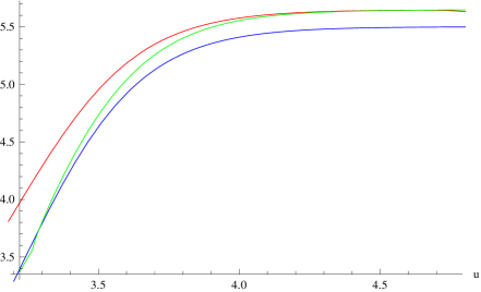
Figure 5: The plots for $a(u)$ (the blue line), the apparent horizon (the green line) and the local event horizon (the red line) in the dynamic process. We have set $g^{2}\,,\tilde{\alpha}\,,\tilde{\gamma}$ to unity and $q_{*}=5\,,Q=1/\sqrt{3}$.

In general, Eq.(47) cannot be solved analytically. We will study it using numerical approach. Without loss of generality, we focus on the $n=4$ dimension. In Fig.5, we plot $a(u)$ as a function of the advanced time $u$. It is clear that the space-time evolves from some unstable states in which the power-law singularity at the origin was dressed by an apparent horizon. This is characteristic for our charged solutions. At the future infinity, the space-time approaches the equilibrium and arrives at stationary black hole states. We also see that both the apparent horizon and the local event horizon monotonically increase with the advanced time and approach the event horizon of the final black holes at the future infinity.

In addition, the Vaidya mass satisfies

$$\dot{M}={\textstyle{\frac{\scriptstyle(n-2)^{2}}{\scriptstyle 64(n-1)\pi}}}a^{n-2}(\tilde{\alpha}+\tilde{\gamma}Q^{2}a^{4-2n})\dot{a}\,.$$ (51)

It follows that $\dot{M}>0$ in the whole dynamic process since $\dot{a}>0$, implying that the Vaidya mass also monotonically increases with the advanced time.

At the future infinity, the system approaches the static limit at an exponential rate of $e^{-u/u_{0}}$. We find

$$a=q\big{(}1-c_{0}e^{-{\frac{u}{u_{0}}}}+{\textstyle{\frac{\scriptstyle 3-(2n-7)\log x}{\scriptstyle 2(1+\log x)}}}c_{0}^{2}e^{-{\frac{2u}{u_{0}}}}+\cdots\big{)}\,,$$

$$M=M_{0}\Big{(}1-{\textstyle{\frac{\scriptstyle(n-3)(n-1)(1+\log x)}{\scriptstyle n-3-(n-1)\log x}}}c_{0}e^{-{\frac{u}{u_{0}}}}+{\textstyle{\frac{\scriptstyle(n-3)(n-1)\big{(}n+1-3(n-3)\log x\big{)}}{\scriptstyle 2\big{(}n-3-(n-1)\log x\big{)}}}}c_{0}^{2}e^{-{\frac{2u}{u_{0}}}}+\cdots\Big{)}\,.$$ (52)

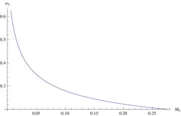
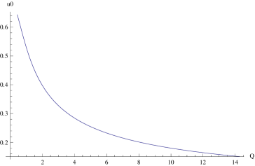
Figure 6: The plots for the relation time $u_{0}$ in the $n=4$ dimension. In the left plot, $u_{0}$ is plotted as a function of the final black hole mass $M_{0}$ for fixing electric charge $Q=1/\sqrt{3}$. In the right plot, it is plotted as a function of the electric charge for fixing black hole mass $M_{0}=1/(48\pi)$. We have set $g^{2}\,,\tilde{\alpha}\,,\tilde{\gamma}$ to unity.

Here $c_{0}$ is a positive integration constant and $M_{0}$ is the mass of the final black holes, given by Eq.(45) with $a$ replaced by $q$. Note that the sub-leading correction of the Vaidya mass requires $\log x<{\textstyle{\frac{\scriptstyle n-3}{\scriptstyle n-1}}}$. This is equivalent to the condition for the positiveness of the final black hole mass. The relaxation time is given by

$$u_{0}={\frac{1}{\tilde{\alpha}q(1+\log x)}}={\frac{1}{q\big{(}\tilde{\alpha}+\tilde{\gamma}Q^{2}q^{4-2n}\big{)}}}\,,$$ (53)

which turns out to be a rather involved and decreasing function of the mass and the electric charge of the final black holes (see Fig.6).

5 Conclusions

In this paper, we study the global properties of some exact dynamical black holes with scalar hair which were found in certain minimally and non-minimally coupled Einstein-scalar gravity. In order to analyze the global structures, we adopt an effective notion “local event horizon” as well as the apparent horizon.

For the solutions of both minimal and non-minimal thoeries, we find that the apparent horizon is always inside the local event horizon in the whole dynamical process and both of them increase monotonically with the advanced time and approach the event horizon at the future infinity. We also find that the apparent horizon smoothly and gradually evolves into a future outer one at the late times of the evolution. This is instructive to support the solutions describing black holes formation. At the future infinity, the solution reaches the static limit exponentially fast with the relaxation time inversely proportional to the $1/(n-1)$ power of the final black hole mass.

There exists a crucial difference in the initial state of the solutions between the minimal and non-minimal theories. For the non-minimal case, the dynamical evolution of the space-time starts from pure AdS vacua which is linearly stable. However, driven by some non-linear effects the space-time spontaneously evolves into stationary black hole states at the future infinity. For the minimal case, the space-time evolves from some finite advanced time (which was set to zero), at which the scalar vanishes. However, the space-time does not become AdS vacua at this point. It contains a power-law singularity at the origin which results to linear instability and triggers the dynamical evolution.

For the non-minimal theory, we also obtain new charged solutions by introducing an additional Maxwell filed which is non-minimally coupled to the scalar. The initial state of the evolution has non-vanishing scalar and becomes unstable at the linear level. This is significantly different from the pure neutral solutions. At the future infinity, the charged solutions also exponentially approach stable black hole states with the relaxation time strongly modified by the electric charge.

References

- [1] A. Anabalon, D. Astefanesei and R. Mann, Exact asymptotically flat charged hairy black holes with a dilaton potential, JHEP 1310, 184 (2013) [arXiv:1308.1693 [hep-th]].
- [2] A. Anabalon, Exact hairy black holes, Springer Proc. Phys. 157, 3 (2014) [arXiv:1211.2765 [gr-qc]].
- [3] P.A. González, E. Papantonopoulos, J. Saavedra and Y. Vásquez, Four-dimensional asymptotically AdS black holes with scalar Hair, JHEP 1312, 021 (2013) [arXiv:1309.2161 [gr-qc]].
- [4] X.H. Feng, H. Lü and Q. Wen, Scalar hairy black holes in general dimensions, Phys. Rev. D 89, no. 4, 044014 (2014) [arXiv:1312.5374 [hep-th]].
- [5] Z. Y. Fan and H. Lu, Charged Black Holes with Scalar Hair, JHEP 1509, 060 (2015) [arXiv:1507.04369 [hep-th]].
- [6] C. A. R. Herdeiro and E. Radu, Kerr black holes with scalar hair, Phys. Rev. Lett. 112, 221101 (2014) [arXiv:1403.2757 [gr-qc]].
- [7] W. J. Geng and H. Lu, Einstein-Vector Gravity, Emerging Gauge Symmetry and de Sitter Bounce, arXiv:1511.03681 [hep-th].
- [8] P. Bizon, Colored black holes, Phys. Rev. Lett. 64, 2844 (1990).
- [9] B. Kleihaus and J. Kunz, Rotating hairy black holes, Phys. Rev. Lett. 86, 3704 (2001) [gr-qc/0012081].
- [10] B. Kleihaus, J. Kunz and F. Navarro-Lerida, Rotating Einstein-Yang-Mills black holes, Phys. Rev. D 66, 104001 (2002) [gr-qc/0207042].
- [11] P. Meessen, Supersymmetric coloured/hairy black holes, Phys. Lett. B 665, 388 (2008) [arXiv:0803.0684 [hep-th]].
- [12] Z. Y. Fan and H. L , SU(2)-Colored (A)dS Black Holes in Conformal Gravity, JHEP 1502, 013 (2015) [arXiv:1411.5372 [hep-th]].
- [13] H. Lu, A. Perkins, C. N. Pope and K. S. Stelle, Black Holes in Higher-Derivative Gravity, Phys. Rev. Lett. 114, no. 17, 171601 (2015) [arXiv:1502.01028 [hep-th]].
- [14] H. L , A. Perkins, C. N. Pope and K. S. Stelle, Spherically Symmetric Solutions in Higher-Derivative Gravity, Phys. Rev. D 92, no. 12, 124019 (2015) [arXiv:1508.00010 [hep-th]].
- [15] M. Henneaux, C. Martinez, R. Troncoso and J. Zanelli, Black holes and asymptotics of 2+1 gravity coupled to a scalar field, Phys. Rev. D 65, 104007 (2002) [hep-th/0201170].
- [16] C. Martinez, R. Troncoso and J. Zanelli, Exact black hole solution with a minimally coupled scalar field, Phys. Rev. D 70, 084035 (2004) [hep-th/0406111].
- [17] A. Anabalon and D. Astefanesei, On attractor mechanism of black holes, Phys. Lett. B 727, 568 (2013) [arXiv:1309.5863 [hep-th]].
- [18] A. Acena, A. Anabalon, D. Astefanesei and R. Mann, Hairy planar black holes in higher dimensions, JHEP 1401, 153 (2014) [arXiv:1311.6065 [hep-th]].
- [19] K.G. Zloshchastiev, On co-existence of black holes and scalar field, Phys. Rev. Lett. 94, 121101 (2005) [hep-th/0408163].
- [20] Z. Y. Fan and H. Lu, Static and Dynamic Hairy Planar Black Holes, Phys. Rev. D 92, no. 6, 064008 (2015) [arXiv:1505.03557 [hep-th]].
- [21] X. Zhang and H. Lü, Exact black hole formation in asymptotically (A)dS and flat spacetimes, Phys. Lett. B 736, 455 (2014) [arXiv:1403.6874 [hep-th]].
- [22] X. Zhang and H. Lü, Critical behavior in a massless scalar field collapse with self-interaction potential, Phys. Rev. D 91, no. 4, 044046 (2015) [arXiv:1410.8337 [gr-qc]].
- [23] H. Lü and X. Zhang, Exact collapse solutions in gauged supergravity and their generalizations, JHEP 1407, 099 (2014) [arXiv:1404.7603 [hep-th]].
- [24] W. Xu, Exact black hole formation in three dimensions, Phys. Lett. B 738, 472 (2014) [arXiv:1409.3368 [hep-th]].
- [25] E. Ayón-Beato, M. Hassaïne and J. A. Méndez-Zavaleta, (Super-)renormalizably dressed black holes, Phys. Rev. D 92, no. 2, 024048 (2015) [arXiv:1506.02277 [hep-th]].
- [26] Z. Y. Fan and B. Chen, Exact formation of hairy planar black holes, arXiv:1512.09145 [hep-th].
- [27] Z. Zhao and X. X. Dai, A New method dealing with Hawking effects of evaporating black holes, Mod. Phys. Lett. A 7, 1771 (1992).
- [28] Z. Zhao, J. H. Zhang and J. Y. Zhu, Quantum thermal effect of arbitrarily accelerating Kinnersley black hole, Int. J. Theor. Phys. 34, 2039 (1995) [Int. J. Mod. Phys. A 20, 1353 (2005)].
- [29] A. Wang, No-Go Theorem in Spacetimes with Two Commuting Spacelike Killing Vectors, Gen. Rel. Grav. 37, 1919 (2005)
- [30] S.J. Gates, Jr. and B. Zwiebach, Gauged supergravity theory with a new scalar potential, Phys. Lett. B 123, 200 (1983).