Interval Estimation for the ‘Net Promoter Score’

Abstract

The Net Promoter Score (NPS) is a novel summary statistic used by thousands of companies as a key performance indicator of customer loyalty. While adoption of the statistic has grown rapidly over the last decade, there has been little published on its statistical properties. Common interval estimation techniques are adapted for use with the NPS, and performance assessed on the largest available database of companies’ Net Promoter Scores. Variations on the Adjusted Wald, and an iterative Score test are found to have superior performance.

Key words: confidence interval, Net Promoter, net score, NPS, significance test

Satmetrix Systems Inc., 3 Twin Dolphin Dr, Redwood City, CA 94065
e-mail: rocks.brendan@gmail.com

1 The Net Promoter Score

1.1 Usage and Calculation

The Net Promoter Score (NPS) is a summary statistic proposed by Reichheld (2003; 2006), commonly used in commercial survey research to estimate the propensity of a business’ customers to exhibit desirable behaviors, such as recommending friends, or spending a greater share of their income (Owen & Brooks, 2008; Reichheld, 2011). General practice is to ask the question “How likely is it that you would recommend Company X to a friend or colleague?”, with responses captured on a 0 to 10 Likert scale. The NPS statistic is then calculated as follows; respondents who rate 0 to 6 are classified as Detractors, 7 or 8 as Passives, and 9 or 10 as Promoters. The NPS is calculated as the percentage of Promoters, less the percentage of Detractors, producing a score between -1 and 1.

We’ll consider the number of respondents in each category a vector of length three, $x=[x_{det},\>x_{pas,\>}x_{pro}]$, with their relative proportions the corresponding probability vector $p=[p_{det},\>p_{pas,\>}p_{pro}]$, the score itself being $NPS=p_{pro}-p_{det}$. The score may also be reached by recoding Promoter, Passive and Detractor responses as 1, 0, and -1, respectively, and taking the arithmetic mean.

This paper focuses on estimating intervals for the $NPS$ statistic itself, as opposed to other measures which might describe the trinomial distribution used to derive it. This is an important distinction; a single $NPS$ can come from many (potentially rather different) distributions.

1.2 Critiques

A variety of metrics thought to predict customer behaviors exist within marketing, and Riechheld’s (2003) claim that the $NPS$ is superior has been challenged by several authors. In particular, on the grounds that $NPS$ and alternative metrics have similar relationships to business-outcomes (Van Doorn et al. 2013; Pingitore et al. 2007; Keiningham et al. 2007b); that an 11-point Likert scale may not be the optimal measurement instrument (Schneider et al. 2008); and that multiple measures combined and weighted via a regression model provide better predictions (Keiningham et al. 2007a). Compared to taking the mean on the original scale, the novel calculation has been argued to both lose information (Eskildsen and Kristensen 2011), and improve performance in predicting customer retention (De Haan et al. 2015). Despite these critiques, the Net Promoter Score is used to estimate customer sentiment by thousands of companies (Owen and Brooks 2008; Reichheld 2011). This paper investigates its statistical properties.

1.3 Properties

Many possible trinomial probability mass distributions (TPMDs) can result in an $NPS$ of 0, half that number for an $NPS$ of $\frac{1}{2}$, and only 1 for an $NPS$ of 1 (or -1). For any $n$, there are $2n+1$ possible Net Promoter scores, the distribution having a peak 1 score wide at 0, with $n$ ‘steps’ of two scores width either side for even $n$, and a peak of 3 scores wide, with $n-1$ steps for odd numbered $n.$

Unlike the [0,1] uniform distribution of possible values of a binomial proportion, possible values of the $NPS$ from a simplex lattice follow a triangular distribution ($a=1,b=-1,c=0$) as $n$ approaches infinity.

This is an important distinction with regard to assessing interval methods; performance averaged uniformly across possible TPMDs is not performance averaged uniformly over Net Promoter Scores (Figure 1).

Testing a method for $NPS$ with equal weight across TPMDs, means that (for example) performance at $NPS=0$ will have twice the weight of performance at $NPS=\frac{1}{2}$, as for arbitrary trinomial distributions, an $NPS$ of $0$ is twice as likely to occur.

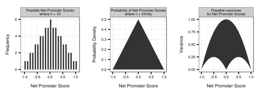
Figure 1: Illustrations of Net Promoter Scores drawn from simplex lattices. The left panel illustrates the discrete distribution of possible Net Promoter Scores for $n=10$. The center panel shows the smooth triangular distribution when $n$ approaches infinity - the binomial equivalent would be uniform. The rightmost panel shows the range of possible Net Promoter Scores and variances for infinite $n$, the possible distributions being uniformly distributed within the inverted shield shape.

1.4 Variance of the NPS

Methods for the variance of the difference of two proportions can be applied to the $NPS$ (e.g. Gold, 1963; Goodman, 1965)

$$\sigma_{NPS}=p_{pro}+p_{det}-(p_{pro}-p_{det})^{2},$$

with the variance ranging from 0 (all respondents in the same category, for example Passives), to a maximum of 1 (data equally split between Promoters and Detractors). It’s worth noting that these two extreme examples would both produce an $NPS$ of 0; unlike a binomial proportion, we cannot derive an $NPS$ from its variance.

2 Interval estimation

2.1 Wald Intervals, and Variations

2.1.1 The Wald Interval

A commonly taught and used method for sample proportions is the Wald confidence interval (first proposed by Laplace, 1812), $p\pm z_{\alpha/2}\sqrt{p(1-p)/n}$, where $z_{\alpha/2}$ denotes the $1-(\alpha/2)$ quantile of a standard normal distribution. It is straightforward to use the variance calculation (1) to produce a Wald interval for the $NPS$:

$$NPS\pm z_{\alpha/2}\sqrt{\frac{\sigma_{NPS}}{n}}.$$ (1)

2.1.2 The Goodman method

Goodman (1964), proposed a method for estimating net differences between multinomial parameters. It functions in a similar form to the Wald interval, with the sample $NPS$ forming the central point of the interval

$$\pm\sqrt{\chi\frac{\sigma_{NPS}}{n}}$$

where $\chi$ is the upper $(a/K)\times 100th$ percentile of the $\chi^{2}$ distribution with one degree of freedom.

2.1.3 The Adjusted Wald

The ‘Adjusted Wald’ test proposed by Agresti & Coull (1998) in its original binomial form is to perform the Wald test, after the adjustment of adding $\frac{z_{\alpha/2}^{2}}{2}$ to the number of successes, and $z_{\alpha/2}^{2}$ to the number of trails. Similarly, Agresti & Min (2005) proposed an Adjusted Wald for matched pairs in $2\times 2$ contingency table designs.

We can adapt this to the $NPS$ by adding $\frac{z_{\alpha/2}^{2}}{3}$ to the number of respondents in each category, so that $\hat{x}=x+\frac{z_{\alpha/2}^{2}}{3}$, and $\hat{n}=n+z_{\alpha/2}^{2}$, making our adjusted estimate of the TPMD $\hat{p}=\frac{\hat{x}}{\hat{n}}$, the new central estimate $\widehat{NPS}=\hat{{p}}_{pro}-\hat{{p}}_{det}$, and new variance $\hat{\sigma}_{NPS}=\hat{{p}}{}_{pro}+\hat{{p}}_{det}-(\hat{{p}}_{pro}-\hat{{p}}_{det})^{2}$. We then use these adjusted parameters to create intervals using the Wald method in 1 above:

$$\widehat{NPS}\pm z_{\alpha/2}\sqrt{\frac{\hat{\sigma}_{NPS}}{\hat{n}}.}$$

These adjustments shrink the estimated TPMD towards the uniform, the additions to $\hat{x}$ bringing $\widehat{NPS}$ closer to 0, and the estimated variance closer to $\frac{2}{3}$.

The weights added to $x$ need not necessarily sum to $z_{\alpha/2}^{2}$, or be equally distributed across the trinomial categories. Agresti & Coull (1998) proposed a total weight of 4 (as opposed to $z_{\alpha/2}^{2}$). Agresti & Min’s (2005) specification for matched-pairs advocates adding the same weight to each of the four categories in a $2\times 2$ table, which when respecified for a TPMD, can be considered adding twice the weight to $p_{pas}$ than is added to $p_{pro}$ and $p_{det}$. This does not affect the central estimate of the interval, but has the effect of reducing the estimated variance and interval width.

Bonett & Price (2012) suggested another novel adjustment for the Wald, again in the context of matched pairs and $2\times 2$ tables, which is to add the weight to just the cells subject to the statistic’s calculation - in our case, the weight split equally between the trinomial extremes of $p_{pro}$ and $p_{det}$.

Notation for Adjusted Wald Interval Estimates

This paper uses the notation $AW(w,shape)$ to denote an Adjusted Wald interval, where $w$ is the total weight added to $\hat{x}$, and $shape$ can be extreme (E), triangular (T), or uniform (U); denoting $p_{pas}$ having no weight, twice the weight, or the same weight as the other categories, respectively. This results in the prior having a variance of $1$ (for E) $\frac{2}{3}$ (for U) or $\frac{1}{2}$ (for T). For example, an Adjusted Wald interval with one response added to each trinomial category would be denoted $AW(3,U)$. This paper assesses Adjusted Wald 95% intervals where $w$ is equal to $2$, $3$, and $z_{\alpha/2}^{2}$ ($\approx 3.84$), for all three shape types.

2.2 Score Tests

2.2.1 The Score Test

The score test, originally proposed by Wilson (1927) has the binomial formula

$$\left(p+\frac{z_{\alpha/2}^{2}}{2n}\pm z_{\alpha/2}\sqrt{\left[p(1-p)+z_{\alpha/2}^{2}/4n\right]/n}\right)/(1+z_{\alpha/2}^{2}/n).$$ (2)

As presented in Agresti & Coull’s illuminating 1998 paper, the central point of the interval can be alternatively specified as a weighted average, $p(w_{1})+\frac{1}{2}(w_{2})$, the two weights being $w_{1}=\frac{n}{n+z^{2}}$ and $w_{2}=\frac{z^{2}}{n+z^{2}}$ respectively. This weighted average shrinks $\hat{p}$ towards $\frac{1}{2}$, with this effect diminishing as $n$ increases. Standard errors either side of this midpoint are $z_{\alpha/2}\sqrt{\frac{p(1-p)w_{1}+\frac{1}{4}w_{2}}{n+z^{2}}}$, providing a weighted average between the sample variance, and the maximum possible variance of $\frac{1}{4}$.

Using the the weighted average principle, we can adapt this to the $NPS$, with the two weights shrinking the central estimate towards 0 as opposed to $\frac{1}{2}$, as follows:

$$\widehat{NPS}=\left(NPS+1\right)w_{1}+w_{2}-1,$$

The formula for the intervals,

$$\widehat{NPS}\pm z_{\alpha/2}\sqrt{\frac{\sigma_{NPS}w_{1}+w_{2}}{n+z^{2}}}$$ (3)

is similar in form to the original Wilson score test, but with the weighted average drawing the variance towards the $NPS$ maximum of 1. This prior variance can be altered by the addition of a multiplier to $w_{2}$; in this paper prior variances of $\frac{2}{3}$ and $\frac{1}{2}$ are tested, to provide equivalence with the prior variances of the uniform and triangular Adjusted Wald tests.

2.2.2 The Iterative Score Method

Inverting the score test was first proposed for paired sample designs, and applications to $2\times 2$ tables by Tango (1998). This test can be reinterpreted to cover the $NPS$ of a trinomial distribution. Modifying Agresti & Min’s (2005) presentation, its interval would be the set of values $\Delta$, satisfying

$$\frac{|(NPS)-\Delta|}{\sqrt{\frac{(\tilde{p}_{pro}(\Delta)+\tilde{p}_{det}(\Delta))-\Delta^{2}}{n}}}<z_{\alpha/2}$$

where $\tilde{p}_{i}(\Delta)$ is the MLE of $p_{i}$, under the constraint $\Delta=NPS$. This can be solved iteratively; for this paper, the implementation was adapted from code for the Tango (1998) method by Agresti (2003).

2.2.3 The May-Johnson Score Method

May & Johnson (1997) proposed a closed form version of Tango’s method, again originally intended for $2\times 2$ tables from matched pairs designs. It can be adapted to trinomial data and the $NPS$ as follows

$$NPS\left(\frac{n}{\hat{n}}\right)\pm z_{\alpha/2}\sqrt{\frac{\hat{n}(p_{pro}+p_{det})-n(p_{pro}-p_{det})^{2}}{\hat{n}}}$$

where $\hat{n}=n+z_{\alpha/2}^{2}$.

2.3 Similarity Between Methods

The Score Method, May-Joshnson Score Method, and Adjusted Wald tests with a weight of $z_{\alpha/2}^{2}$, all produce identical central estimates for the interval. Both the Goodman and Wald methods take the sample $NPS$ as the central estimate.

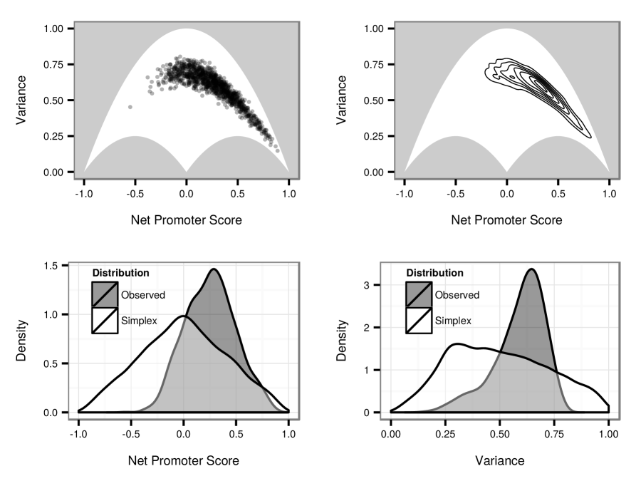
Figure 2: The $NPS$ and variance of the 1,098 observed TPMDs from the Satmetrix data set, illustrated with a scatter plot (upper left panel), and contour plot (upper right panel) of the two-dimensional kernel density estimate. The area outside the range of possible distributions is shaded gray. Marginal density estimates from the same model for the $NPS$ (lower left panel), and variance (lower right panel) are also shown, compared to those from the samples from the simplex lattice. Compared to the range of possible TPMDs, those observed have higher mean Net Promoter Scores and variances, and are much more tightly grouped.

3 Assessment of Coverage Probabilities

3.1 Methods

The methods of Agresti & Coull (1998) inform the simulation based approach for coverage probability assessment. The specified confidence level of a procedure is compared to the long run average of times that a procedure’s interval contains the ‘true’ population parameter, when supplied data from a random sample of the population. For the this analysis, the nominal confidence level chosen is 95%. This means that the results indicate average, as opposed to worst possible performance; procedures where coverage probabilities are greater than the nominal confidence level will be seen as overly conservative, those with lower than nominal coverage probabilities will be seen as overly liberal.

3.1.1 Arbitrary Trinomial Distributions

Trinomial probability mass distributions were generated by randomly sampling $J=10,000$ points from a (3, 400) simplex lattice. Performance at each TPMD was assessed at 20 $n$ counts; $2\times 10^{5}$ trinomial distributions in total. Performance at each trinomial distribution was assessed with 10,000 simulations. This is a sample of trinomial distributions from those which are arbitrarily possible.

3.1.2 Observed Trinomial Distributions

While sampling from a simplex lattice gives a good indication of performance over possible distributions, in psychometric practice, some distributions are more likely than others. The Satmetrix US Consumer Net Promoter Study (Rocks, 2015) is the largest available database of companies’ Net Promoter Scores. Aggregating at the interaction of year-of-response and company, 347,788 Likelihood to Recommend ratings for 236 companies over 14 years yielded 1,098 trinomial Net Promoter distributions (with at least 250 responses). The data illustrate that samples from a simplex lattice are not an ideal model of human response behaviors (Figure 2). The observed TPMDs have much more narrowly distributed Net Promoter Scores (mean = .26, standard deviation = .24) and variances (mean = .59, standard deviation = .12) than the simplex lattice samples, and occupy a relatively small small area of the possible parameter space.

Performance more likely to be observed in practice

To create statistics which reflect performance across values sampled from the simplex lattice, performance is averaged across the $J$ TPMDs sampled from it. For statistics which might better reflect performance in practice, we can make this a weighted average, the weights reflecting how frequently such a TPMD has been observed. To create these weights, a two-dimensional kernel density estimate was fit to the $NPS$ and variance of the trinomial distributions observed in the Satmetrix data-set , the weights being the density estimate of a given distribution (rescaled so that the sum of the weights across the $J$ samples is 1). This paper presents performance both with and without these observational weights applied.

3.1.3 Desirable Performance Characteristics

In addition to a test having an average coverage level close to 95%, the following characteristics are desirable:

• Good performance across values for $n$, especially $\leqslant 100$

• Low variation in performance across trinomial distributions. For example, a test may have an average coverage probability of 95%, by returning extremely conservative results for certain distributions, and extremely liberal results for others

• Good performance for both the observed and simplex distributions

A convenient summary of these properties is the mean absolute error (MAE) of the test, defined at a particular $n$ value, as

$$MAE=\frac{\sum(C_{j}-0.95)w_{j}}{\sum w_{j}}$$

where $C_{j}$ is the coverage probability of the test for the $j^{th}$ TPMD sampled from the simplex lattice, and $w_{j}$ is the weight for that distribution. The tests’ MAE for $n\leqslant 100$ will be used as our ultimate criteria for recommendation. This paper considers performance both with, and without ($w_{1,\ldots,J}=\frac{1}{J}$) observational weights applied to the MAE.

Table 1: A coverage probability heat map for the different interval estimation methods varying with sample $n$ counts, for the observed (left panel) and simplex (right panel) distributions. Tests are ordered by average coverage probability for the observed distribution, where $n\leqslant 100$. Coverage probabilities below $90\%$ are filled solid black with white text.

3.2 Results

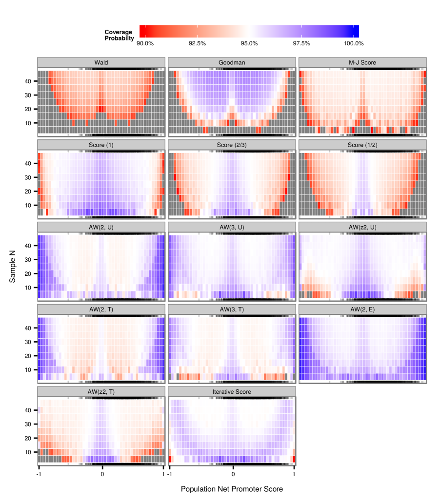
Figure 3: A coverage probability heat map for the different interval estimation methods, with varying Net Promoter Scores and $n$ counts. Rug plots above and below each panel illustrate the observed distribution of Net Promoter Scores. Coverage probabilities below $90\%$ are shaded gray.

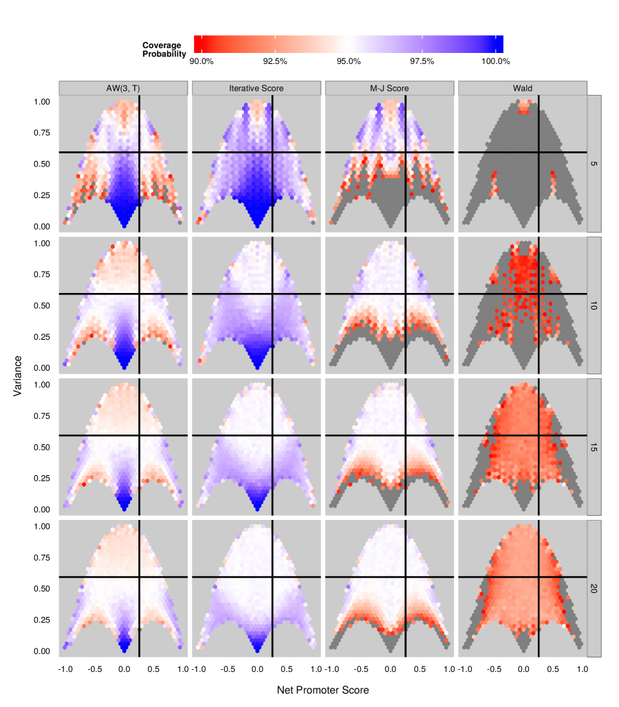
Figure 4: Coverage probabilities for the $AW(3,T)$, Iterative Score, May-Johnson Score, and Wald methods, across the TPMD parameter space, for varying $n$. The mean $NPS$ and variance of the observed distribution is indicated on each small multiple with cross-hairs. Areas with coverage probabilities below 90% are shaded dark gray. Note that for the $AW(3,T)$, the area around the mean of the bivariate distribution is closest to its region of optimal performance, compared to the Iterative Score, where it is in a region of conservative bias.

Table 1 shows the average coverage probabilities for the tests at 95% intervals. The tests share the same general characteristic of performance closer to the nominal level with increasing $n$, the exception being the Goodman method. It produces intervals which are too small with low $n$, and to wide with large $n$, the test passing through the nominal coverage level at $n$ of around 20 for the simplex distribution.

The Wald test for $NPS$ fares better than its binomial equivalent in Agresti & Coull (1998), though performance is still overly liberal. Coverage improves with increasing $n$, though doesn’t quite reach the nominal 95% level by $n=300$.

Table 2: Mean Absolute Error (multiplied by 100 for presentational purposes) and rank, for interval estimation methods, for both the simplex and observed distributions. Tests are ordered by descending total MAE for the observed distribution, where $n\leqslant 100$.

The May-Johnson Score test has the best average coverage probability for the observed distribution. However, this comes at the expense of variation in performance (illustrated in Figure 3), which is rather high, the coverage probability falling to below 90% at $n=5$ on the simplex distribution, and being overly liberal at extreme and central $NPS$ values at low $n$.

Weighted Average Variations on the Score Test

For the ‘weighted average’ variations on the Wilson type score tests, drawing the variance towards $\frac{1}{2}$ and $\frac{2}{3}$ produces an on-average improvement in coverage probability over the original specification of a prior variance of 1 (Table 1). Unfortunately, this comes at the expense of greater variance in performance across Net Promoter Scores at low $n$ (Figure 3).

Variations on the Adjusted Wald

All Adjusted Wald methods are superior to the Wald, with the $AW(3,T)$ the best of those tested, on both the observed and simplex distributions. For the observed distribution, it has the lowest MAE for $n\leqslant 100$ of any test, and the second lowest for the simplex (Table 2), very little coverage below the nominal level (Figure 3), and superb average coverage probabilities (Table 1), for both the observed and simplex distributions.

The Iterative Score

The Iterative Score method also has excellent performance. Summing MAE for all $n$, it has the lowest total for the simplex distribution, and its performance is very rarely over-liberal, the test returning coverage below 90% the least frequently of any considered (less than 0.01% of simplex samples), and having the highest minimum coverage observed in the simulations (83%). However, it has the disadvantage of being overly conservative at low n. Like the Adjusted Wald tests, it’s more conservative at the extremes of $NPS$ for small $n$.

Performance with varying n

Our main performance statistic for recommending a test (MAE for $n\leqslant 100$) contains an intentional bias, in that it favors tests which have better performance at low $n$ values, where MAE tends to be higher, making a greater contribution to the aggregate. The $AW(3,T)$ benefits from this the most, having better relative performance for observed and simplex distributions at $n$ below around 15 and 20, respectively.

An alternative statistic might be to rank our tests’ performance at each value of $n$, and then select the method with the lowest average rank. For the simplex distribution, using this criteria makes little difference, with the Iterative Score, followed by the $AW(3,T)$ having the lowest average rank. However, for the observed distribution, the $AW(3,T)$ falls to eighth place, with the May-Johnson score coming out the best, followed by the $AW(z_{\alpha/2}^{2},T)$.

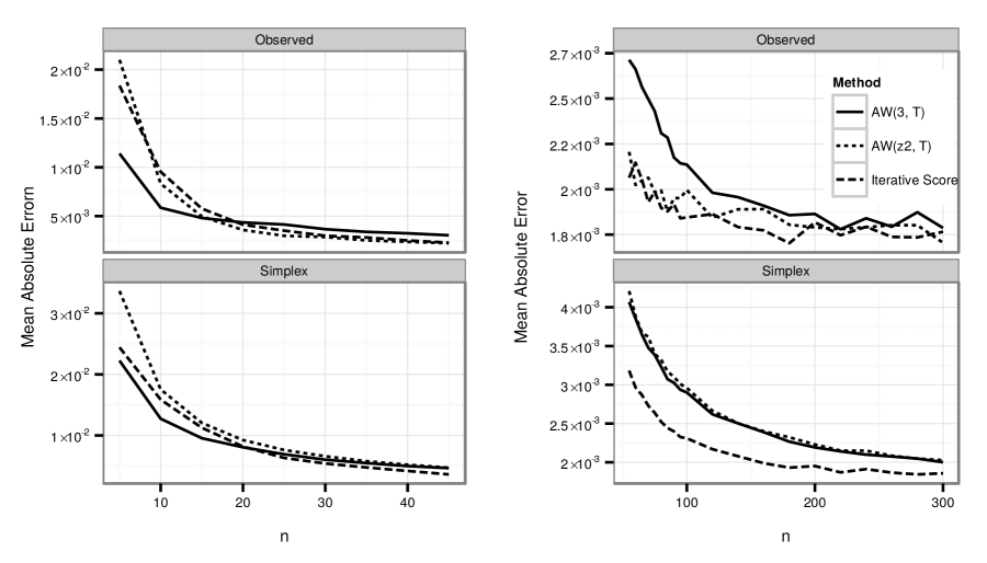
Figure 5: Mean Absolute Error with varying $n$, for the Iterative score, AW(3, T), and AW$(z_{\alpha/2}^{2}$, T) tests.

Of course, $n$ counts are known at the time of interval construction; it is possible to select the best performing test at any of the intervals for $n$ analyzed in this paper, or create a single ‘method’ where the underlying calculations change based on the total $n$. However, doing so offers extremely modest performance improvements (reducing the MAE by $4.09\times 10^{-4}$ and $5.38\times 10^{-4}$ for the simplex and observed distributions respectively).

The difference between the MAEs of the tests decreases rapidly with $n$, meaning that there is very little difference in MAE between the ranks after around $n=30$. Figure 5 illustrates this pattern, the $AW(3,T)$ having superior performance, when differences in performance are of the highest magnitude.

Observed vs. Simplex distributions

Our choice of two distributions provides us with two different sets of results to judge our tests by. It’s clear from the observational data (Figure 2) that performance in a relatively small region of parameter space is of much greater importance under the conditions observed. Figure 4 illustrates the overlap of observational data and coverage probability in parameter space, explaining the large increase in performance in the $AW(3,T)$ and May-Johnson Score tests that are seen on the observed vs. simplex distributions.

The observations have been selected to be representative of US Consumers using the standard survey methodology, and thus perhaps the data generating mechanism from which practitioners are most likely to encounter the $NPS$. However, response behaviors are known to vary by both industry and country (Owen & Brooks, 2008), and interval estimation methods may be applied to ‘net proportion’ statistics outside of traditional data collection for a Net Promoter Score. Performance on both distributions are presented here, and it is left to the reader to select the best test for their particular application.

3.3 Additional Confidence Levels

While the 95% confidence interval is perhaps the most commonly used, an important consideration for a test is performance at a range of common confidence levels. The analysis above was replicated for a subset of tests (the Iterative Score, the Score $\left(\frac{2}{3}\right)$, the $AW(3,T)$, and the $AW(z^{2},T)$), for 99%, 90% and 80% confidence intervals. The tests represent the best performing test of each type (closed-form score, Adjusted Wald, and Iterative score) at 95% confidence, with the addition of the $AW(z^{2},T)$, which varies weights based on $\alpha$.

Results are presented in Table 3. Averaged across confidence levels and $n$ values, the test with the lowest $MAE$ remains the $AW(3,T)$ for the observed distribution, and the Iterative Score for the simplex distribution. However, these averages are affected by the higher $MAE$ seen in lower confidence levels. Results vary, with tests which were generally liberal at 95% performing better at lower confidence levels, and vice versa. Averaging $MAE$ across $n$, the best test for the 99% level on both distributions is the Iterative Score, followed by the $AW(3,T)$. For 80% and 90% confidence levels, the best performing test is the Score $\left(\frac{2}{3}\right)$ for the observed distribution, and the $AW(z^{2},T)$ for the simplex.

Table 3: Mean Absolute Error of estimation methods (multiplied by 100 for presentational purposes) and rank, for the simplex and observed distributions across confidence levels. Tests are ordered by descending total MAE for the observed distribution, where $n\leqslant 100$.

4 Conclusion & Summary

The Wald and Goodman tests perform poorly; their use should be avoided. All Adjusted Wald variations considered provided substantial improvement, with the best of those (weights of $3$ and $z_{\alpha/2}^{2}$) outperforming non-iterative Score methods.

The best performing Adjusted Wald is $AW(3,T)$ which can be used by adding $\frac{3}{4}$ to the counts of both Promoters and Detractors, and $\frac{3}{2}$ to the count of Passives, before construction of a Wald interval. The method has good performance across the $n$ values and confidence levels examined, especially for data likely to be observed in practice.

The Iterative Score method also has excellent performance, with the advantage that it has very few regions of parameter space where coverage drops below 95%, providing accurate coverage probabilities for almost any trinomial distribution. Its disadvantage is its greater computational complexity, and slight conservatism at low $n$ values ($<20$ for a 95% interval) for trinomial distributions likely to be observed in practice.

5 Acknowledgements

The author would like to thank two anonymous reviewers and an assistant editor for comments which greatly helped improve this manuscript.

6 Trademark Information

Net Promoter, Net Promoter Score, and NPS are trademarks of Satmetrix Systems, Inc., Bain & Company, Inc., and Fred Reichheld.

References

- Agresti (2003) Agresti, A. (2003) R2 matched. URLhttp://www.stat.ufl.edu/ aa/cda/R/matched/R2_matched/. [Online; accessed 2014-12-20].
- Agresti and Coull (1998) Agresti, A. and Coull, B. A. (1998) Approximate is better than “exact” for interval estimation of binomial proportions. The American Statistician, 52, 119–126.
- Agresti and Min (2005) Agresti, A. and Min, Y. (2005) Simple improved confidence intervals for comparing matched proportions. Statistics in Medicine, 24, 729–740.
- Bonett and Price (2012) Bonett, D. G. and Price, R. M. (2012) Adjusted wald confidence interval for a difference of binomial proportions based on paired data. Journal of Educational and Behavioral Statistics, 37, 479–488.
- Chacón and Duong (2010) Chacón, J. E. and Duong, T. (2010) Multivariate plug-in bandwidth selection with unconstrained pilot bandwidth matrices. Test, 19, 375–398.
- De Haan et al. (2015) De Haan, E., Verhoef, P. C. and Wiesel, T. (2015) The predictive ability of different customer feedback metrics for retention. International Journal of Research in Marketing, 32, 195–206.
- Duong (2014) Duong, T. (2014) ks: Kernel Smoothing. URLhttp://cran.r-project.org/package=ks.
- Eskildsen and Kristensen (2011) Eskildsen, J. K. and Kristensen, K. (2011) The accuracy of the net promoter score under different distributional assumptions. In Quality, Reliability, Risk, Maintenance, and Safety Engineering (ICQR2MSE), 2011 International Conference on, 964–969. IEEE.
- Gold (1963) Gold, R. Z. (1963) Tests auxiliary to 2 tests in a Markov chain. Annals of Mathematical Statistics, 34, 56–74.
- Goodman (1964) Goodman, L. A. (1964) Simultaneous confidence intervals for contrasts among multinomial populations. The Annals of Mathematical Statistics, 35, 716–725.
- Goodman (1965) — (1965) On simultaneous confidence intervals for multinomial proportions. Technometrics, 7, 247–254.
- Huber (2011) Huber, W. (2011) How can i calculate margin of error in a nps (net promoter score) result? URLhttp://stats.stackexchange.com/a/18609. [Online; accessed 2014-12-20].
- Keiningham et al. (2007a) Keiningham, T. L., Cooil, B., Aksoy, L., Andreassen, T. W. and Weiner, J. (2007a) The value of different customer satisfaction and loyalty metrics in predicting customer retention, recommendation, and share-of-wallet. Managing Service Quality: An International Journal, 17, 361–384.
- Keiningham et al. (2007b) Keiningham, T. L., Cooil, B., Andreassen, T. W. and Aksoy, L. (2007b) A longitudinal examination of net promoter and firm revenue growth. Journal of Marketing, 71, 39–51.
- de Laplace (1812) de Laplace, P. S. (1812) Théorie analytique des probabilités. Paris, France: Courcier.
- May and Johnson (1997) May, W. L. and Johnson, W. D. (1997) Confidence intervals for differences in correlated binary proportions. Statistics in Medicine, 16, 2127–2136.
- Owen and Brooks (2008) Owen, R. and Brooks, L. L. (2008) Answering The Ultimate Question: How Net Promoter can Transform your Business. New Jersey, USA: John Wiley & Sons.
- Pingitore et al. (2007) Pingitore, G., Morgan, N. A., Rego, L. L., Gigliotti, A. and Meyers, J. (2007) The single-question trap. Marketing Research, 19.
- Reichheld (2003) Reichheld, F. F. (2003) The one number you need to grow. Harvard Business Review, 81, 46–55.
- Reichheld (2006) — (2006) The ultimate question. Harvard Business School Press.
- Reichheld (2011) — (2011) The Ultimate Question 2.0: How Net Promoter Companies Thrive in a Customer-Driven World. Boston, USA: Harvard Business Press.
- Rocks (2015) Rocks, B. (2015) The Satmetrix 2015 us consumer net promoter study. URLhttp://www.satmetrix.com/net-promoter/industry-benchmarks/. [Online; accessed 2015-01-15].
- Schneider et al. (2008) Schneider, D., Berent, M., Thomas, R. and Krosnick, J. (2008) Measuring customer satisfaction and loyalty: Improving the ‘net-promoter’ score. In Poster presented at the Annual Meeting of the American Association for Public Opinion Research, New Orleans, Louisiana.
- Tango (1998) Tango, T. (1998) Equivalence test and confidence interval for the difference in proportions for the paired-sample design. Statistics in Medicine, 17, 891–908.
- Van Doorn et al. (2013) Van Doorn, J., Leeflang, P. S. H. and Tijs, M. (2013) Satisfaction as a predictor of future performance: A replication. International Journal of Research in Marketing, 30, 314–318.
- Wilson (1927) Wilson, E. B. (1927) Probable inference, the law of succession, and statistical inference. Journal of the American Statistical Association, 22, 209–212.