Extending the Coyote emulator to dark energy models with standard - parametrization of the equation of state.
Abstract
We discuss an extension of the Coyote emulator to predict non-linear matter power spectra of dark energy (DE) models with a scale factor dependent equation of state of the form . The extension is based on the mapping rule between non-linear spectra of DE models with constant equation of state and those with time varying one originally introduced in ref. [40]. Using a series of N-body simulations we show that the spectral equivalence is accurate to sub-percent level across the same range of modes and redshift covered by the Coyote suite. Thus, the extended emulator provides a very efficient and accurate tool to predict non-linear power spectra for DE models with - parametrization. According to the same criteria we have developed a numerical code that we have implemented in a dedicated module for the CAMB code, that can be used in combination with the Coyote Emulator in likelihood analyses of non-linear matter power spectrum measurements. All codes can be found at https://github.com/luciano-casarini/pkequal.
1 Introduction
The origin of cosmic acceleration is scarcely understood. No doubt however remains that the Universe is close to spatially flat (curvature parameter ), while baryons and Dark Matter (DM) only account for of the critical density, errors hardly exceeding [1]. Accordingly, we infere the gap to be filled by a component, or phenomenon, called Dark Energy (DE) and responsible for the observed accelerated expansion [2, 3].
DE could be Einstein’s cosmological constant and/or arise from vacuum quantum fluctuations, being so equivalent to a fluid with state parameter . This simple CDM scenario meets a plenty of cosmic data, well beyond background composition, at least above middle size galactic mass scales. But this does not allow us to forget the mess of conceptual problems going with it, first of all that quantum field theory predicts a vacuum energy exceeding the phenomenological value by orders of magnitudes.
An alternative to is a self–interacting scalar field [5, 6, 7, 8], possibly interacting with DM, as well. Moreover, General Relativity (GR) has no independent test on the huge scales where acceleration is measured, so DE could just arise from large scale GR violations (for comprehensive review see, e.g.,[9]).
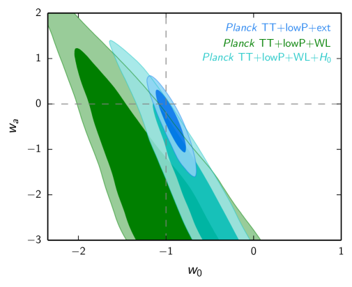
Selecting among different options requires fresh data which, however, are hard to collect. The Planck experiment suggests at [1], if is assumed to be constant. If however one assumes DE state parameter to be consistent with the expression [11, 12]
| (1.1) |
and tests it against the same data, it turns out that at , as also shown by the small ellypse at the center of Figure 1. (We will refer to eq. (1.1) as CPL parametrization.) Clearly results still significantly depend on the range of models tested.
As shown by [13], the CPL expression (and alike) is not exempt of pitfalls either. Moreover, Figure 1 indicates that some tension exists between Planck outputs and CFHTLensS weak lensing data 222Canada France Haway Telescope Lensing Survey [15], leadind to include values in the likelihood ellypse, for which a CPL parametrization [eq. (1.1)] looses significance [14].
Although it is licit to suspect that some systematics pollutes such CMB–lensing comparison, these outputs make evident that weak lensing can be a basic tool to improve our DE knowledge. In fact, while CMB measurement errors have approached cosmic variance limits, so that planned future experiments are essentially meant to improve our knowledge on the inflationary era, the upcoming generation of tomographic lensing surveys, such as LSST333http://www.lsst.org/lsst/ and the Euclid experiment [16], can be expected to measure the power spectrum of matter density fluctuations, , across a wide range of scales and redshifts, up to accuracy. Such accuracy level is therefore the natural target for spectral predictions.
On the very large length scales linear codes match such requirement. Perturbation theory can then extend predictions to the mild non–linearity area; in fact, aiming at a per-cent level, even on the scales of BAO we cannot neglect non-linear dynamics (see e.g. [17]).
At larger ’s, only N-body simulations can provide model predictions. They however demand a significant effort to overcome ambiguities due to sample variance, dependence on the box size and long-wavelength mode contributions, resolution and dynamical range across the entire model parameter space. In turn, this excludes N-body simulations to be part of an “on line” algorithm evaluating model likelihood. Accordingly, future galaxy survey data analyses require reliable and readily available spectral predictions from N–body simulations.
This is why emulators are built, exploring a grid of models by varying a set of parameters, and based on wide set of simulations with different box sizes, resolution etc., for each grid element, so to minimize the impact of the overmentioned N–body simulation problems.
The Coyote emulator [35, 36, 37, 38], in particular, is based on a suite of spatially flat simulations and provides 1 accuracy level estimates of spectra up to (at greater baryon physics matters more than 1), for the following parameter range
Here , while and are the dimensionless Hubble parameter and the density parameters for baryons and DM, respectively; is the spectral index for primeval scalar perturbations; is the m.s. amplitude of density fluctuations on the 8Mpc scale. For a given value of and the reduced Hubble constant is set to reproduce the location of the CMB peaks in the temperature anisotropy power spectrum. The effective number of neutrino species is however assumed to be through the whole suite.
In this work we shall show how the Coyote emulator can be extended to models with a CPL DE state parameter [eq. (1.1)] without any significant accuracy degrade. To do so, we shall follow the pattern outlined in some previous papers [40, 41, 42] extending the approach of [43], also adding a specific evaluation of the shifts on the admitted range of , which depends on the – values considered. Thanks to the width of the intervals explored by the Coyote simulation suite, the evaluated limits (we shall plot them accurately in a forthcoming Section, for a specific choice of ’s and ) will be shown to include all physically relevant – models and, in particular, those inside the 2– ellypse at the center of Fig. 1. In connection with this work, we also provide a code, to be associated to the Coyote emulator, allowing one to predict spectra for – cosmologies without significant accuracy degrade.
In this work we shall also consider a fully different approach to detect fluctuation spectra, based on the halo model and first followed by [18]. Their analysis gradually evolved into the Halofit expressions [19] furtherly extended by [20] and were also included in the CAMB code [21]. Along the same pattern, massive neutrinos models, and an update for modified gravity models [29, 30] were included respectively in [22] and [23].
Beside Halofit, a standard halo model [24, 25] fitting formula was provided by [26] were baryons effects were tentatively included by using the simulations of [27]. Then [28] went still forward, providing predictions for a number of more complex cases. They include models with massive neutrinos, gravity models, including those yielding Chamaleon or Vainshtein screening [31, 32], and DM– coupling described by the equations
| (1.2) |
fulfilled by stress–energy tensors of DM and DE; apices (c) and (d), respectively; these models were first simulated by [34] and later by [33] who also treated the case of . In spite of such a wide range of cosmologies, the halo model exhibits its effectiveness by providing fair predictions, with an accuracy . Although still far from the desired 1 limit, this is a significant step forward to cover the domain that experiments will be testing.
Letting however apart these extensions, in association to this work we also provide a code to be used together with the CAMB package, enabling one to extend [20] results for constant , to any – cosmology, without any appreciable accuracy degrade.
The paper is organized as follows. In Section 2 we will review the mapping rule between model parameters and [40], providing explicit codes to implement it. In Section 3 we test the validity of the spectral equivalence using results from a set of N-body simulations. In Section 4 we discuss the physical origin of the spectral equivalence and compare results from different model mapping criteria. Section 5 is then devoted to a precise determination of CPL models to which the Coyote emulator can be extended.
2 Non-Linear Matter Power Spectrum and Model Equivalence
Numerical studies of structure formation show signatures of DE state equation on a number of non–linear observables, as the halo mass function [49, 50, 51], the density profile of DM halos [50, 52, 53] and, namely, fluctuation spectra [44, 45, 46, 40, 47, 48]. This comes as no surprise as DE alters the late linear growth. In turn, in an expanding background, the equations of motion for a system of collisionless particles are almost model independent if the linear growth factor is used as time-variable [54].
These arguments provide the physical basis to estimate the non-linear spectra of a given target model at a given redshift , from N-body simulations of an equivalent or auxiliary model . In fact, [43] showed that – and constant– cosmologies exhibit close spectra at if, besides of sharing the cosmological parameters and (density parameters for baryons, matter, DM, reduced Hubble parameter, primeval scalar spectral index and m.s. fluctuation amplitude on the scale of 8Mpc at , respectively), they also exhibit an identical comoving distance between and the last scattering surface (LSB). Moreover, according to [43], for some – choices, there exists a greater redshift where and are again equidistant from the LSB. Spectral discrepancies, keeping within up to Mpc-1 at , grow up to in the 0– interval; they tend again to decrease in the proximity of , becoming wider and wider at still greater redshift. Aiming at 1 accuracy, [40] tried to extend the criterion at each , seeking –dependent auxiliary models .
First of all we require that all models share target model and parameter values at . This soon implies and to share the reduced density parameters at any , even though and are different. Then, if we want to determine the value of and the present normalization amplitude of the power spectrum in model , such that both models have the same non-linear power spectra at redshift as shown in [40] this requires imposing two conditions.
First, by demanding that and have the same distance to the last scattering surface one can infer the value of by numerically solving the equation:
| (2.1) |
where is the redshfit when last scattering surface occurs, , and
| (2.2) |
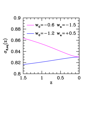
Secondly, having determined we can derive the value of in from the value of in by imposing that the amplitude of the density fluctuations at the scale of Mpc h-1 at redshift is the same in both models:
| (2.3) |
where the linear growth factor is the growing mode solution to the linear perturbation equation:
| (2.4) |
For a given set of values of and these two conditions give at each redshift a unique value of and .
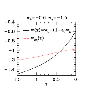
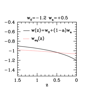
In former work [40, 41, 42] the validity of this criterion was tested for a wide range of models. Here, for the sake of example, Fig. 2 shows tests concerning two different target models , close to the edge of contours of the smallest ellipse at the center of Fig. 1.
A fortran program, called PKequal, computing the values of and at a given redshift for any given target model can be downloaded from the following link https://github.com/luciano-casarini/pkequal. This program was used, e.g., to obtain Fig. 2.
3 N-body Simulation Tests
In this Section we provide details on the tests run for this work, aimed at comparing the power spectra from N-body simulations of target and auxiliary models in and about the parameter range covered by the Coyote emulator. Particle distributions generated at by graphic2 [56] were evolved down to by using the tree–code pdkgrav [55]. Matter power spectra were then obtained at various redshifts through the code PMpowerM, included in the PM package described in [57], performing a Cloud-in-Cell interpolation of the particle distribution to reconstruct the density field on a uniform cartesian grid, with a maximum number of cells.
Simulations were run in boxes with various box sizes and particle numbers, yielding different values for the Nyquist frequency , mostly considered a fair estimate of the maximum where simulations are numerically reliable. At an accuracy level , this however needs to be verified. The simulations used to obtain the results in Figures 3 and 4 are shown in the Table
Their names shown in the first column are meant to remind and .
This selection of simulation parameters is aimed to test the effects of longer wavelength modes and small scale resolution on the discrepancies between target and auxiliary models, for which we aim at reaching a precise scale and redshift dependence.
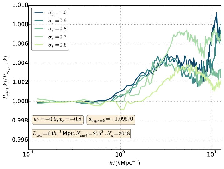
Here below we shall illustrate results for a CPL target model with , , , and, namely, and , treated also in Figure 2. Those related to the other extreme of the likelihood ellipse are mostly analogous and we shall just outline the differences we found.
In Coyote’s range the auxiliary models of such cosmology have state parameter ranging from () to -1.1863 (), as also shown in Fig. 2. These values are close to the center of the -interval covered by the Coyote emulator. A set of values, ranging from 0.6 to 1, were considered. Results will be shown in Figure 3.
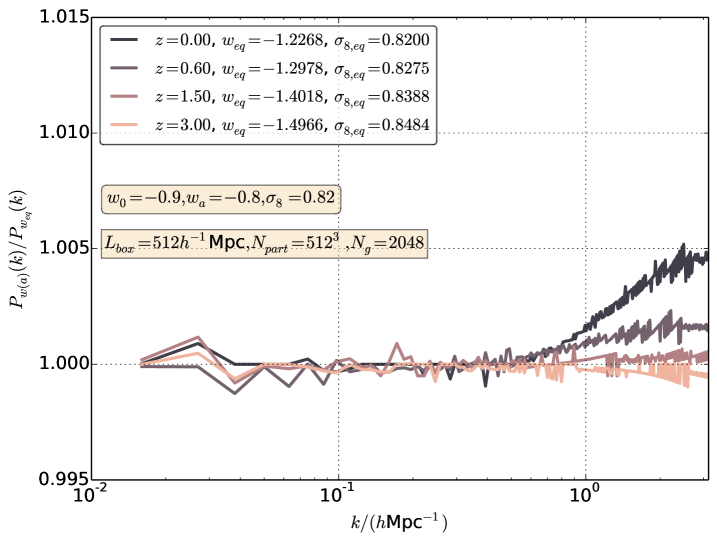
We however went forward and, in Figure 4, will show results for redshifts up to although for a unique target model with .
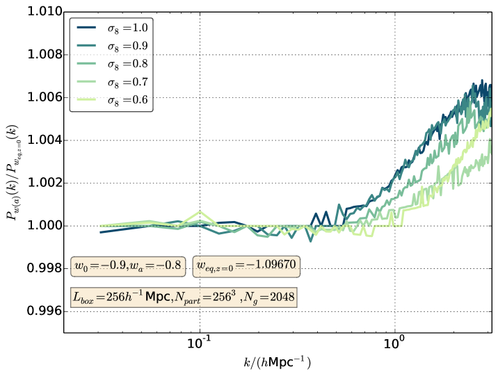
From all simulations we derive ratios between matter power spectra of target and auxiliary models at where, according to previous analysis, discrepancies reach their maximum. In the top panel of Figure 3 we plot such ratio, as derived from , up to at for different values of 444Notice that at we have . Up to Mpc-1, for , discrepancies essentially overlap. For (0.6) they are slightly (significantly) smaller. Until Mpc-1 they never exceed ; they then approach () at Mpc -1 ( Mpc -1). It should be also outlined that, at Mpc -1, the discrepancy growth tends to stop, never bypassing .
The bottom panel of Fig. 3 is derived from . Longer wavelength modes are therefore included, at the expenses of a smaller resolution, although however exceeds Mpc-1. Model discrepancies appear slightly greater here than in , approaching at Mpc-1 while however keeping below for Mpc-1. This is associated to a start of discrepancies at a slightly lower than in in .
There seem to be scarce doubts that the latter tiny effect arises from the contribution of long wavelength discrepancies. On the contrary, comparison with the next Figure will confirm that the bulk of the former slight increase is to be attributed to being already too close. Even including such a tiny numerical noise effect, however, the limit for Mpc-1 is kept.
Let us finally comment the discrepancies in . Although restricted to at , Figure 4 shows, first of all, how discrepancies decrease with increasing , becoming apparent only for . It is however worth outlining that, in the case of the model with , , discrepancies do not dye so early. This is due to the greater values of , only partially balanced by decreasing –instead of increasing, see Figure 2– with . Even in this case, however, no residual discrepancy can be appreciated above .
Apart of that, we may compare the discrepancies at with those for in the previous Figure. This allows us to appreciate, first of all, that doubling the volume side does not modify at all the range above which discrepancy exhibit their mild increase, i.e, longer wave have no more impact on that. Then, at –Mpc-1, we recognize almost identical details, hence presumably deriving from the approaching of identical Nyquist frequencies. Although bearing no impact on the discrepancy limits for Mpc-1, this makes us believe that, in this region, the top panel of Fig. 3 may be more reliable than the bottom one.
Altogether we can conclude that residual model discrepancies increase with (while decreasing with ). Being mostly interested here just to Mpc-1 (above such baryon physics requires corrections ) model discrepancies were never seen to exceed . However, if one wishes to use the procedure up to Mpc-1, a safe accuracy limit can be .
4 Physical Origin of Spectral Equivalence
In this Section we shall compare other possible options with the equivalence criterion set by eq. (2.1), which can be also restated as requiring that equal conformal times have elapsed from the LSS to the relevant redshift .
It has been known since long that the conformal time sets the best metric on the time coordinate, over scales involved in the cosmic expansion. Such metric is often used in linear codes (e.g. by CAMB) and primeval sonic waves are (quasi–)periodical in respect to it. Then, as mentioned in [54], the linear growth factor defines a time variable that rescale the dynamical equations of N-body particles in a form that is nearly independent of the underlying cosmological model. Thus, once two models share the same linear growth histories, when N-body particles begin to form non–linearities, the similarity is preserved and eventually leads to similar power spectra.
To show this more clearly, we test the spectral equivalence for two tentative additional DE model mapping criteria, defined as the following.
For a given set of values of and we infer by requiring:
-
•
equality of the linear growth factors at the redshift of interest,
(4.1) -
•
equality of the integral of the linear growth factors up to the redshift of interest,
(4.2)
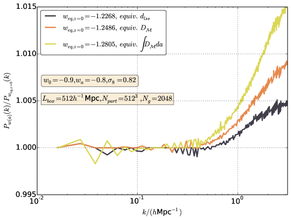
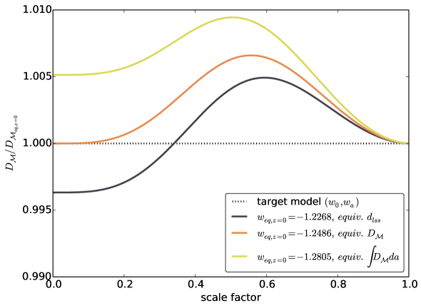
We consider again a target model with and . At it is mapped into an auxiliary model with constant equation of state [, ] for the criterion (2.1) [(4.1), (4.2)]. To test such two additional criteria, we run ad–hoc simulations for each equivalent model defined according to them. We used a Mpc box size, with particles, and set ; the other cosmological parameters are kept equal.
In Figure 5 we plot the ratio of non-linear power spectra at (top panel) of target and auxiliary models for the three different criteria and the ratio of the normalized linear growth factors (bottom panel). This shows that the differences between the non-linear spectra in the high- interval are correlated with deviations of the linear growth histories between target and auxiliary models. The mapping rule based on the equality of the distance to last scattering surface (conformal times) shows the smallest deviations between non-linear spectra as well as the smallest differences of the linear growth factors across the entire cosmic history. In contrast, the criterion based on the integral of the growth factors leads to the largest discrepancies of the spectra as well as the large deviations between the linear growth histories. This clearly indicates that whenever two cosmologies share similar growth factors they should also have similar non-linear power spectra.
This criterion suggests a mapping rule that, in principle, could be extended beyond the case of DE parametrizations, e.g. to Modified Gravity models. This might deserve an accurate future study.
A point outlined in the top panel of Figure 3 is that discrepancies between target and auxiliary models apparently stabilize even when we extend the spectral comparison up to large ’s. Admittedly, this part of computed spectra has no direct phenomenological meaning as, there, baryons cannot be neglected. An open question, however, is whether non–linear baryon dynamics necessarily leads to differentiating otherwise equivalent models which, e.g., share and values; and, if it does so, which are the origin and the size of the expected discrepancies.
5 CPL parameter range of the Coyote emulator
The Coyote emulator provides non-linear power spectra for DE models with constant equation of state. Thus, we can use the spectral model equivalence described in the previous Section to extend the predictions to the CPL parameter space. Here, we determine the range of values of and that for a given value of and at a given redshift have an auxiliary model with values of and in the range covered by the Coyote emulator.
Hereafter, we set , , and which are well within the range probed by the Coyote suite.
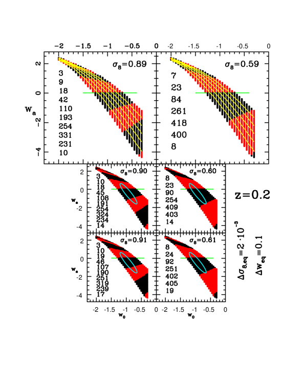
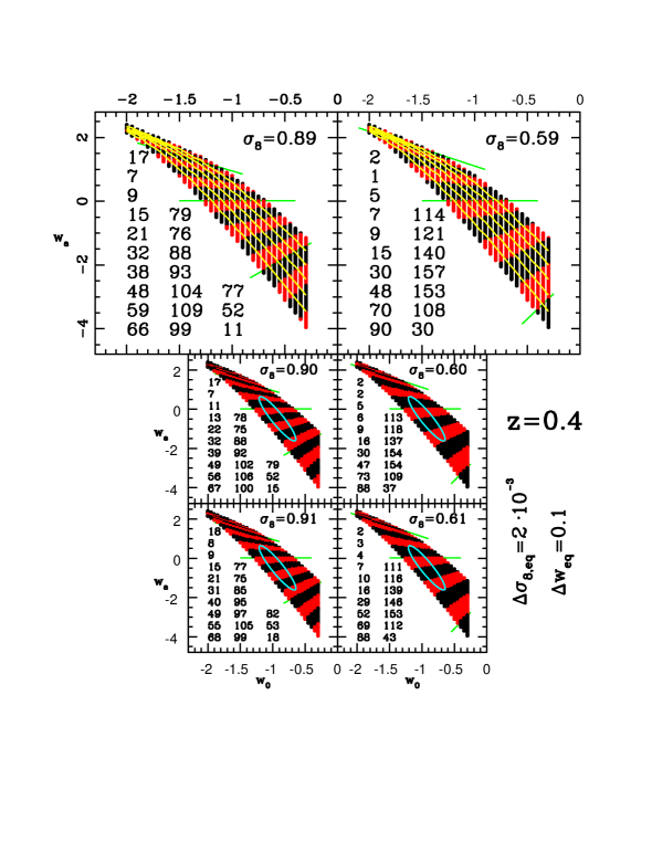
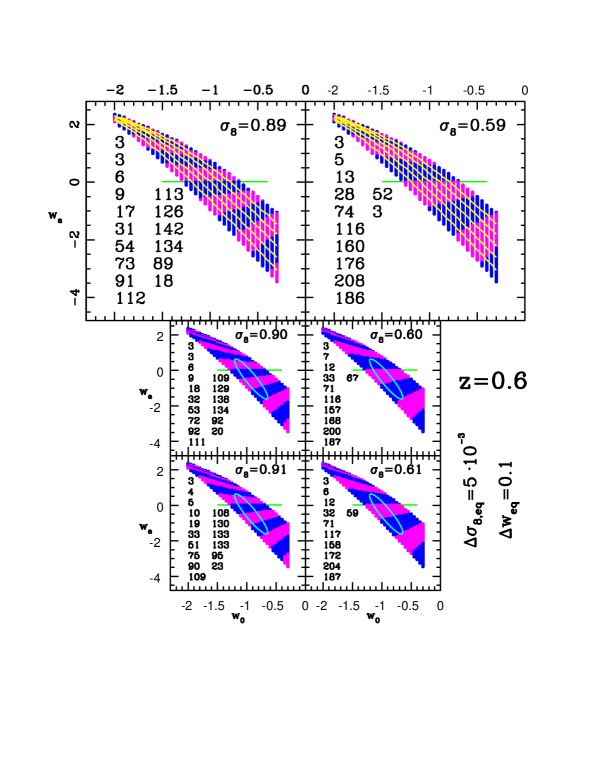
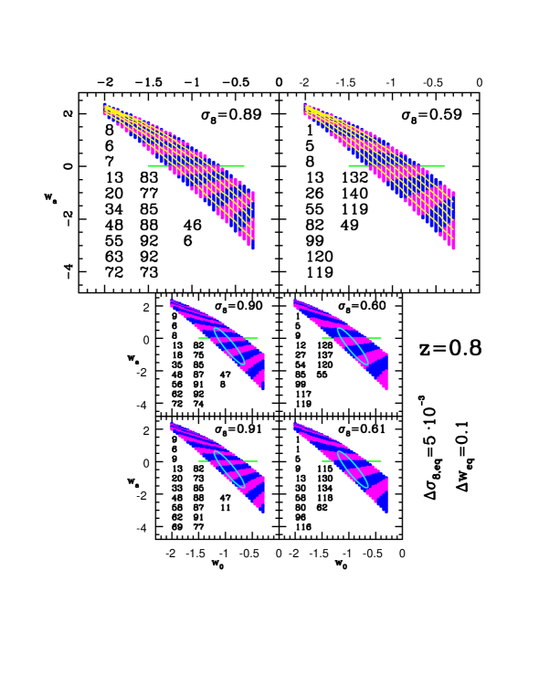
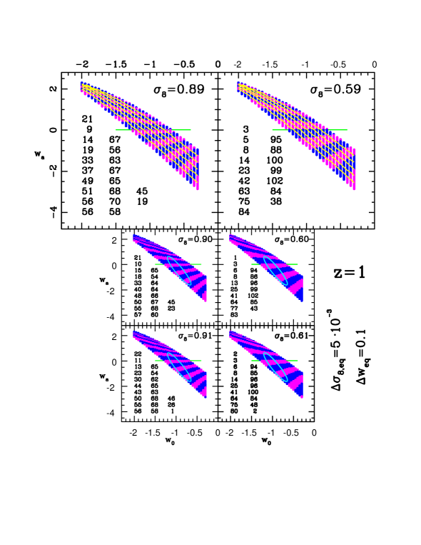
At , we find that all values of and within the countours of the combined Planck data analysis shown in Figure 1 have a counterpart in the Coyote suite. At higher redshift the availability of auxiliary models depends on redshift the specific values of , and as summarized in Figure 6 for (top panel) and (bottom panel), Figure 7 for (top panel) and (bottom panel) and Figure 8 for . In each panel the various plots correspond to different . We specifically focus on values which are at the extreme end of the Coyote interval, since it is in these cases that target models may corresponds to auxiliary ones with values outside the Coyote range. Thus, in the figures we plot region of the CPL parameter space for and respectively.
The information encoded in these plots can be read as the following. Each panel show a region of the - plane (roughly corresponding to the region constrained by the Planck data, see Figure 1) that maps corresponding values of probed by the Coyote emulator. In each panel the values of can be read from the larger plots as a series of nearly parallel yellow lines varying in the range in steps of from bottom to top. The horizontal green lines correspond to the case , where and . The alternating black and red bands above (below) the horizontal green lines correspond to increments (decrements) of the value by for and , and for and respectively. The smaller plots in each panel show the case corresponding to values that are at the limit (or just outside) the range covered by the Coyote emulator. Here, only certain regions of the parameter space have auxiliary models in the Coyote suite, while other have no counterpart includes models that are within the contours from the combined Planck data analysis (represented in the figure by the elliptical contour). Nonetheless, it is worth noticing that such regions are associated with extreme values of and that are more than away from Planck best-fit value.
The various plots have been realized through a discrete sampling of the CPL parameter space in steps of in and . The list of numbers in each plot specifies the number of - pairs for each band of values. In the case we have two additional green lines above and below the horizontal one which mark the shift in the increment (decrement) of by . Notice that the limits shown in Figure 6 to 8 hold when the remaining cosmological parameters are set to fiducial values; we however tested that varying and within current observational uncertainties induces negligible differences. We can conclude that, up to , the bulk of physically significant DE models with CPL parametrization have a counterpart in the ensemble of models originally covered by the Coyote emulator.
6 Comparison with HMcode
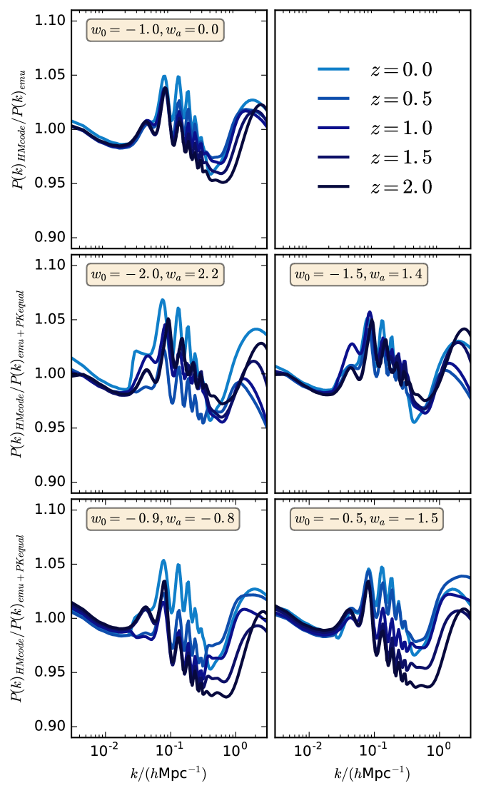
The improved accuracy of our algorithm can be directly appreciated if we compare our results with the fitted Halo model provided by the HMcode recently extended to CPL models [28] 555https://github.com/alexander-mead/HMcode.
In Figure 9, we show a comparison between the power spectra predicted by our code PKequal applied to COSMIC EMU and the HMcode.
As a basic example, let us consider a CDM cosmology, whose equivalent model, obviously, is CDM itself. Let us then compare the results of the HMcode, for this case, directly with the COSMIC EMU. As expected, through the HMcode, we recover the results shown in Fig. 2 of [26]; the predictions of COSMIC EMU, although slightly discrepant, are substantially in agreement with the HMcode at 5 % level, as expected. In order to perform this comparison we considered the node 0 set parameters indicated in Table 1 of [26]: , , , and .
Fig. 9 let us then appreciate the performance of HMcode also for a number of CPL models, mostly inside the precision for and , apart of the case of DE with , at , exhibiting a greater discrepancy in a short interval around . It should be however borne in mind that the HMcode covers models well beyond standard DE, whose state equation has a CPL expression, like coupled DE models and Vainshtein screened modified gravity models.
7 Conclusions
In this work we have first revisited the equivalence criterion proposed by [40], to extend [43] results to any redshift with no accuracy degrade. Such criterion allows us to obtain the spectra of models with state parameter parametrized by the CPL expression (target models) from suitable auxiliary models with constant state parameter. The auxiliary model, and hence the constant state parameter , varies with redshift.
This criterion, already tested in a variety of cases [40, 41, 42], was again verified here for two models at the extremes of the 2– likelihood ellipse set by the Planck experiment on the – plane. Results were shown in detail for , , standard ’s, and parameter values, and a set of values from 0.6 to unity.
Residual discrepancies were so shown to keep within () in the range of modes (3) and for redshifts .
The remarkable precision of this equivalence points to a degeneracy of the imprint of DE on the non-linear matter power power spectrum. This is because the non-linear regime of gravitational collapse, far from erasing information on the past linear growth, rather carries a strong signature of it. Henceforth, since DE nature affects the linear growth of matter density perturbations in the late cosmic expansion, models with similar linear growth histories also show very similar non-linear power spectra. The conditions for the spectral equivalence defined by eqs. (2.1) and (2.3) guarantees to maps models with such properties.
We also compared the model mapping criterion [40] with a few alternative ones and found that it performs best. This result outlines the key role of comoving distance or conformal time in comparing linear (and, henceforth, nonlinear) evolutions.
The essential contribution of this work however concerns a set of new codes, based on this equivalence criterion and now made available. In fact, spectral equivalence allows us to provide an improved emulator extending the predictions of the Coyote suite to the non-linear matter power spectrum of DE models with CPL parametrization.
We have also shown that the whole of the CPL parameter space compatible with [1] cosmological constraints has auxiliary models in the Coyote suite, although high values, marginally compatible with available cosmological limits, are just on the edge of the extended emulator at , for these models where high values find their compensation in strongly negative . Let us also remind that the Coyote emulator, both in the original and our extended versions, works up to at most.
On the contrary, the extended Halofit expressions, also included in the CAMB program, formally work at any and . Accordingly, besides of a code that can be used individually or joined with Coyote Emulator, we developed a module, which can be inserted in the CAMB package, and allows anyone to obtain non linear power spectra for any –, in agreement with our equivalence criterion. This routine, e.g., can be immediately used in likelihood analyses of non-linear matter power spectrum measurements.
Acknowledgments
S.A. Bonometto acknowledges the support of CIFS (Inter–University Center for Space Physics), P.S. Corasaniti is supported by the ERC-StG “EDECS” no. 279954. This work has made use of the computing facilities of National Center for Supercomputing (CESUP/UFRGS), and of the Laboratory of Astroinformatics (IAG/USP, NAT/Unicsul), whose purchase was made possible by the Brazilian agency FAPESP (2009/54006-4) and the INCT-A.
References
- [1] Planck collaboration: P. Ade et al., Planck 2015 results. XIII. Cosmological parameters, arXiv:1502.01589v2
- [2] A. G. Riess et al., Observational Evidence from Supernovae for an Accelerating Universe and a Cosmological Constant, ApJ 116, 1009 (1998)
- [3] S. Perlmutter et al., Measurements of and from 42 High-Redshift Supernovae, ApJ 517, 565 (1999)
- [4] M. Tegmark et al., Cosmological parameters from SDSS and WMAP, Phys. Rev. D 69, 103501 (2004)
- [5] B. Ratra, P.J.E. Peebles, Cosmological consequences of a rolling homogeneous scalar field, Phys. Rev. D37, 3406 (1988)
- [6] C. Wetterich, Cosmology and the fate of dilatation symmetry, Nucl. Phys. B302, 668 (1988)
- [7] J. Ellis, S. Kalara, K.A. Olive & C. Wetterich, Density-dependent couplings and astrophysical bounds on light scalar particles, Phys. Lett. B2 28, 264 (1989)
- [8] R.R. Caldwell, R. Dave, P.J. Steinhardt, Cosmological Imprint of an Energy Component with General Equation of State, Phys. Rev. Lett. 80, 1582 (1998)
- [9] T. Clifton, P.G. Ferreira, A. Padilla, C. Skordis, Modified Gravity and Cosmology, Phys. Rep. 513, 1 (2012), arXiv:1106.2476v3
- [10] I. Maor, R. Brustein, J. McMahon, P.J. Steinhardt, Measuring the Equation-of-state of the Universe: Pitfalls and Prospects, Phys. Rev. D65, 123003 (2002)
- [11] M. Chevallier, D. Polarski, Accelerating Universes with Scaling Dark Matter, Int. J. Mod. Phys. D 10, 213 (2001)
- [12] E. Linder, Exploring the Expansion History of the Universe, Phys. Rev. Lett. 90, 1301 (2003)
- [13] B.A. Bassett, P.S. Corasaniti, M. Kunz, The essence of quintessence and the cost of compression, Astrophys. J. 617, L1 (2004)
- [14] P.S. Corasaniti, E.J. Copeland, A model independent approach to the dark energy equation of state, Phys. Rev. D 67, 063521 (2003)
- [15] T. Erben et al., CFHTLenS: the Canada-France-Hawaii Telescope Lensing Survey - imaging data and catalogue products , Mont. Not. Roy. Astron. Soc., 433, 2545 (2013),arXiv:1210.8156
- [16] R. Laureijs et al., Euclid Definition Study Report arXiv:1110.3193
- [17] Y. Rasera et al., Cosmic-variance limited Baryon Acoustic Oscillations from the DEUS-FUR CDM simulation, Mont. Not. Roy. Astron. Soc., 440, 1420 (2014), arXiv:1311.5662
- [18] J.A. Peacock, S.J. Dodds, Non-linear evolution of cosmological power spectra, Mont. Not. Roy. Astron. Soc. 280, 19 (1996)
- [19] Smith, R. E., et al., Stable clustering, the halo model and non-linear cosmological power spectra, Mont. Not. Roy. Astron. Soc., 341, 1311 (2003)
- [20] R. Takahashi, M. Sato, T. Nishimiki, A. Taruya, M. Oguri, Revising the Halofit Model for the Nonlinear Matter Power Spectrum, ApJ 761, 152 (2012)
- [21] A. Lewis, A. Challinor, A. Lasenby, Efficient computation of CMB anisotropies in closed FRW Models, Astrophy. J. 538, 473 (2000)
- [22] S. Bird, M. Viel, M. G. Haehnelt, Massive neutrinos and the non-linear matter power spectrum, Mont. Not. Roy. Astron. Soc., 420, 2551 (2012)
- [23] G.-B. Zhao, Modeling the Nonlinear Clustering in Modified Gravity Models. I. A Fitting Formula for the Matter Power Spectrum of f(R) Gravity, ApJS, 211, 23
- [24] J. A. Peacock and R. E. Smith, Halo occupation numbers and galaxy bias, Mont. Not. Roy. Astron. Soc. 318, 1144 (2000)
- [25] U. Seljak, Analytic model for galaxy and dark matter clustering, Mont. Not. Roy. Astron. Soc. 318, 203 (2000)
- [26] A. J. Mead et al., An accurate halo model for fitting non-linear cosmological power spectra and baryonic feedback models, Mont. Not. Roy. Astron. Soc. 454, 1958 (2015)
- [27] M. P. van Daalen, J. Schaye, C. M. Booth and C. Dalla Vecchia, The effects of galaxy formation on the matter power spectrum: a challenge for precision cosmology, Mont. Not. Roy. Astron. Soc. 415, 3649 (2011)
- [28] A. J. Mead et al., Accurate halo-model matter power spectra with dark energy, massive neutrinos and modified gravitational forces, Mont. Not. Roy. Astron. Soc. 459, 1468 (2016)
- [29] H. A. Buchdahl, Non-linear Lagrangians and cosmological theory, Mont. Not. Roy. Astron. Soc., 150, 1 (1970)
- [30] H. Wayne and S. Ignacy, Models of f(R) cosmic acceleration that evade solar system tests, Physical Review D, 76, 064004 (2007)
- [31] A. I. Vainshtein, To the problem of nonvanishing gravitation mass, Physics Letters B, 39, 393 (1972)
- [32] G. Dvali, G. Gabadadze and M. Porrati, 4D gravity on a brane in 5D Minkowski space, Physics Letters B, 485, 208 (2000)
- [33] M. Baldi, V. Pettorino, G. Robbers and V. Springel, Hydrodynamical N-body simulations of coupled dark energy cosmologies, Mont. Not. Roy. Astron. Soc. 403, 1684 (2010)
- [34] A. V. Macciò, C. Quercellini, R. Mainini, L. Amendola, S. A. Bonometto Coupled dark energy: Parameter constraints from N-body simulations, Physical Review D, 69, 123516 (2004)
- [35] K. Heitmann, E. Lawrence, J. Kwan, S. Habib, D. Higdon, The Coyote Universe Extended: Precision Emulation of the Matter Power Spectrum, ApJ 780, 111 (2014)
- [36] K. Heitmann, M. White, C. Wagner, S. Habib, D. Higdon, The Coyote Universe I: Precision Determination of the Nonlinear Matter Power Spectrum, ApJ 715, 104 (2010)
- [37] K. Heitmann, D. Higdon, M. White, S. Habib, B. J. Williams, C. Wagner, The Coyote Universe II: Cosmological Models and Precision Emulation of the Nonlinear Matter Power Spectrum, ApJ 705, 156 (2009)
- [38] E. Lawrence, K. Heitmann, M. White, D. Higdon, C. Wagner, S. Habib, B. Williams The Coyote Universe III: Simulation Suite and Precision Emulator for the Nonlinear Matter Power Spectrum, ApJ 713, 1322 (2010)
- [39] S. Agarwal et al., PkANN - II. A non-linear matter power spectrum interpolator developed using artificial neural networks, Mont. Not. Roy. Astron. Soc. 439, 2102 (2014)
- [40] L. Casarini, A.V. Macció, S.A. Bonometto, Dynamical dark energy simulations: high accuracy power spectra at high redshift, JCAP 3, 14 (2009)
- [41] L. Casarini, High-precision spectra for dynamical Dark Energy cosmologies from constant-w models, JCAP 8, 5 (2010)
- [42] L. Casarini, Spectra of dynamical dark energy cosmologies from constant- w models, New Astron. 15, 575 (2010)
- [43] M.J. Francis, G.F. Lewis, E.V. Linder, Power Spectra to 1 Accuracy between Dynamical Dark Energy Cosmologies, Mont. Not. Roy. Astron. Soc. 380, 1079 (2007)
- [44] C.-P. Ma, R.R. Caldwell, P. Bode, L. Wang, The mass power spectrum in quintessence cosmological models, Astrophys. J. 521, L1 (1999)
- [45] P. McDonald, H. Trac, C. Contaldi, Dependence of the non-linear mass power spectrum on the equation of state of dark energy, Mont. Not. Roy. Astron. Soc. 366, 547 (2006)
- [46] Z. Ma, The Nonlinear Matter Power Spectrum, Astrophys. J. 665, 887 (2007)
- [47] J.-M. Alimi et al., Imprints of Dark Energy on Cosmic Structure Formation. I. Realistic Quintessence Models, Mont. Not. Roy. Astron. Soc. 401, 775 (2010)
- [48] E. Jennings, C.M. Baugh, R.E. Angulo, S. Pascoli, Simulations of quintessential cold dark matter: beyond the cosmological constant, Mont. Not. Roy. Astron. Soc. 401, 2181 (2010)
- [49] P. Bode, N.A. Bahcall, E.B. Ford, J.P. Ostriker, Evolution of the Cluster MAss Function: GPC3 Dark Matter Simulations, Astrophys. J. 551, 15 (2001)
- [50] A. Klypin, A.V. Macció, R. Mainini, S.A. Bonometto, Halo Properties in Models with Dynamical Dark Energy, Astrophys. J. 559, 31 (2003), arXiv:astro-ph/0303304
- [51] J. Courtin et al., Imprints of dark energy on cosmic structure formation: II) Non-Universality of the halo mass function, Mont. Not. Roy. Astron. Soc. 440, 1911 (2011)
- [52] K. Dolag et al., Numerical study of halo concentrations in dark energy cosmologies, Astron. & Astrophys. 416, 853 (2004)
- [53] C. De Boni et al., Hydrodynamical simulations of galaxy clusters in dark energy cosmologies - I. General properties, Mont. Not. Roy. Astron. Soc. 415, 2758 (2011)
- [54] A. Nusser, J.M. Colberg, The Omega dependence in equations of motion, Mont. Not. Roy. Astron. Soc. 294, 457 (1998)
- [55] J.G. Stadel, Cosmological N-body simulations and their analysis, PhD thesis, University of Washington (2001)
- [56] E. Bertschinger, Multiscale Gaussian Random Fields and Their Application to Cosmological Simulations, Astrophys. J. Suppl. 137, 1 (2001)
- [57] A. Klypin, J. Holtzman, Particle-Mesh code for cosmological simulations, astro-ph/9712217 (1997)