Optimal Auctions with Convex Perceived Payments

Amy Greenwald
Department of Computer Science
Brown University
amy@cs.brown.edu
   Takehiro Oyakawa
Department of Computer Science
Brown University
oyakawa@cs.brown.edu
   Vasilis Syrgkanis
Microsoft Research, NYC
vasy@microsoft.com
Abstract

Myerson derived a simple and elegant solution to the single-parameter revenue-maximization problem in his seminal work on optimal auction design assuming the usual model of quasi-linear utilities. In this paper, we consider a slight generalization of this usual model—from linear to convex “perceived” payments. This more general problem does not appear to admit a solution as simple and elegant as Myerson’s.

While some of Myerson’s results extend to our setting, like his payment formula (suitably adjusted), and the observation that “the mechanism is incentive compatible only if the allocation rule is monotonic,” others do not. For example, we observe that the solutions to the Bayesian and the robust (i.e., non-Bayesian) optimal auction design problems in the convex perceived payment setting do not coincide like they do in the case of linear payments. We therefore study the two problems in turn.

Myerson finds an optimal robust (and Bayesian) auction by solving pointwise: for each vector of virtual values, he finds an optimal, ex-post feasible auction; then he plugs the resulting allocation, which he first verifies is monotonic, into his payment formula. This strategy relies on a key theorem, that expected revenue equals expected virtual surplus, which does not hold in our setting. Still, we derive an upper and a heuristic lower bound on expected revenue in our setting. These bounds are easily computed pointwise, and yield monotonic allocation rules, so can be supported by Myerson payments (suitably adjusted). In this way, our bounds yield heuristics that approximate the optimal robust auction, assuming convex perceived payments.

In tackling the Bayesian problem, we derive a mathematical program that improves upon the default formulation in that it has only polynomially-many payment variables; however, it still has exponentially-many allocation variables and ex-post feasibility constraints. To address this latter issue, we also study the ex-ante relaxation, which requires only polynomially-many constraints, in all. Specifically, we present a closed-form solution to a straightforward relaxation of this relaxation. Then, following similar logic, we present a closed-form upper bound and a heuristic lower bound on the solution to the (ex-post) robust problem. As above, the resulting allocation rules can then be supported by Myerson payment rules, yielding faster heuristics than the greedy ones for approximating the optimal robust auction. Interestingly, all our closed-form solutions are rather intuitive: they allocate in proportion to values (or virtual values).

We close with experiments, the final set of which massages the output of one of the closed-form heuristics for the robust problem into an extremely fast, near-optimal heuristic solution to the Bayesian optimal auction design problem.

1 Introduction

In a seminal paper, Myerson [8] provides a simple and elegant solution to a fundamental problem in optimal auction design: the single-parameter revenue-maximization problem, assuming quasi-linear utilities with linear payments: i.e., ui=vixipisubscript𝑢𝑖subscript𝑣𝑖subscript𝑥𝑖subscript𝑝𝑖u_{i}=v_{i}x_{i}-p_{i}, where vi>0subscript𝑣𝑖0v_{i}>0 is i𝑖i’s private value, xisubscript𝑥𝑖x_{i} is his allocation, and pisubscript𝑝𝑖p_{i} is his payment to the auctioneer. Generally speaking, xisubscript𝑥𝑖x_{i} and pisubscript𝑝𝑖p_{i} are not expressed in the same units; hence, we can think of visubscript𝑣𝑖v_{i} as a conversion factor, converting units of the good being allocated into units of payment (often, money). In this paper, we investigate the extent to which Myerson’s observations carry over to the case of convex “perceived”111There are two potential payments for bidders to consider in auction problems: those paid to the auctioneer, and those subtracted from vixisubscript𝑣𝑖subscript𝑥𝑖v_{i}x_{i} in the bidders’ utility functions. In general, these two payments need not be equated. While we choose to label the former payments (made to the auctioneer) “actual,” and the latter, “perceived,” we could just as well have taken the perspective of the bidders in our naming, and referred to the former as “perceived,” and the latter as “actual.” We also considered referring to perceived payments instead as “costs” instead of payments, which they rightfully are. But as our results include a payment formula for these costs which closely relates to Myerson’s original payment formula, it seemed that qualifying the term payment would be more illuminating. payments. Specifically, we consider utilities of the form ui=vixiqi(pi)subscript𝑢𝑖subscript𝑣𝑖subscript𝑥𝑖subscript𝑞𝑖subscript𝑝𝑖u_{i}=v_{i}x_{i}-q_{i}(p_{i}), where qisubscript𝑞𝑖q_{i} is a convex function that describes payments that i𝑖i perceives, which we distinguish from pisubscript𝑝𝑖p_{i} itself (i𝑖i’s “actual” payment to the auctioneer). Although our results apply to any convex function qisubscript𝑞𝑖q_{i}, as a concrete running example throughout this paper, we assume qi(pi)=pi2subscript𝑞𝑖subscript𝑝𝑖superscriptsubscript𝑝𝑖2q_{i}(p_{i})=p_{i}^{2}, for all bidders i𝑖i.

Our problem formulation is motivated by a reverse auction setting in which a government with a fixed budget is offering subsidies (in euros, say) to power companies in exchange for a supply of renewable energy (in watts, say). We assume the power companies’ utility functions take this form: ui=xiqi(pi)/visuperscriptsubscript𝑢𝑖subscript𝑥𝑖subscript𝑞𝑖subscript𝑝𝑖subscript𝑣𝑖u_{i}^{\prime}=x_{i}-q_{i}(p_{i})/v_{i}, where xisubscript𝑥𝑖x_{i} is some fraction of the total budget in euros, and pisubscript𝑝𝑖p_{i} is some deliverable amount of power in watts. As already mentioned, visubscript𝑣𝑖v_{i} is a conversion factor, in this case from euros to watts. The assumption that qi(pi)subscript𝑞𝑖subscript𝑝𝑖q_{i}(p_{i}) is convex reflects the fact that energy production costs may not be linear; for example, because of diseconomies of scale, it may be the case that as more energy is produced, further units become more and more expensive to produce.

Note that multiplying uisuperscriptsubscript𝑢𝑖u_{i}^{\prime} by visubscript𝑣𝑖v_{i} yields a more familiar utility function—that of the forward auction setting: ui=vixiqi(pi)subscript𝑢𝑖subscript𝑣𝑖subscript𝑥𝑖subscript𝑞𝑖subscript𝑝𝑖u_{i}=v_{i}x_{i}-q_{i}(p_{i}), with utility measured in units of power, rather than money. From this point of view, defining perceived payments qi(pi)=pi2subscript𝑞𝑖subscript𝑝𝑖superscriptsubscript𝑝𝑖2q_{i}(p_{i})=p_{i}^{2} can be interpreted as an assumption of risk aversion. A power company might be risk averse because it might be concerned that it has overestimated its own value, or it might worry that the government won’t actually deliver on the promised subsidies.

Another problem which also fits into our framework is the problem of allocating a fixed block of advertising time to retailers during the Superbowl. In this application, an advertiser’s utility is calculated by converting its allocation, in time, into dollars via its private value, and then subtracting the cost of production: ui=vixiqi(pi)subscript𝑢𝑖subscript𝑣𝑖subscript𝑥𝑖subscript𝑞𝑖subscript𝑝𝑖u_{i}=v_{i}x_{i}-q_{i}(p_{i}). Here, dividing by visubscript𝑣𝑖v_{i} yields the utility function uisuperscriptsubscript𝑢𝑖u_{i}^{\prime}, which, under the assumption that qi(pi)=pi2subscript𝑞𝑖subscript𝑝𝑖superscriptsubscript𝑝𝑖2q_{i}(p_{i})=p_{i}^{2}, again yields the interpretation that production costs are convex; for example, it may be the case that an advertisement that is three times as long as another takes nine times as long to produce.

In both of these problems, the auctioneer’s objective is to maximize its total revenue: 𝔼𝐯[ipi]subscript𝔼𝐯subscript𝑖subscript𝑝𝑖\operatorname*{\mathbb{E}}_{\mathbf{v}}[\sum_{i}p_{i}], where 𝐯=(v1,,vn)𝐯subscript𝑣1subscript𝑣𝑛\mathbf{v}=(v_{1},\ldots,v_{n}) is distributed according to some commonly known joint distribution. Specifically, in the energy problem, the government’s objective is to maximize the amount of power produced, subject to its budget constraint. In the advertising problem, the television network is seeking to maximize its revenue for selling a fixed block of advertising time during the Superbowl (or any other television program).

Summary of Results

In our setting, in which perceived payments are convex, some of Myerson’s observations, such as “the mechanism is incentive compatible only if the allocation rule is monotonic,” continue to hold. So does his payment formula (suitably adjusted).

But others do not. The solutions to the robust (i.e., non-Bayesian) and Bayesian optimal auction design problems (in the latter, incentive compatibility and individual rationality need only hold in expectation) do not coincide in our setting like they do in the linear-payment setting. Moreover, bidder surplus is no longer an upper bound on revenue, and expected revenue no longer equals expected virtual surplus.

We do show, however, that revenue can be upper bounded by a quantity we call pseudo-surplus, and that expected revenue can be heuristically lower bounded by expected virtual surplus. Because it is straightforward to compute these bounds (i.e., greedy algorithms suffice), we propose the following heuristic procedure for the robust optimal auction design problem: 1. solve greedily for a feasible allocation that achieves the upper or heuristic lower bound, and 2. plug that allocation into Myerson’s payment formula to ensure incentive compatibility and individual rationality. We show experimentally that the performance of these heuristics can be near-optimal, and that they are faster than solving the corresponding revenue-maximizing mathematical programs using standard solvers.

Our heuristic that lower bounds the solution to the robust optimal auction design problem also heuristically lower bounds the Bayesian problem, because in the latter the constraints are strictly weaker. Regardless, we prove a theorem for the Bayesian setting that allows us to simplify the revenue-maximizing mathematical program from one that has exponentially-many payment variables to one that has only polynomially-many.

Even so, a Bayesian optimal auction still involves exponentially-many allocation variables and requires satisfying exponentially-many ex-post feasibility constraints. To address this latter concern, we also study the ex-ante relaxation, which requires only polynomially-many constraints, in all. Specifically, we present a closed-form solution to a straightforward relaxation of this relaxation, which yields a closed-form upper bound on the ex-ante Bayesian problem. Intuitively, this solution allocates in proportion to virtual values.

Lastly, following similar logic, we present a closed-form upper bound and a heuristic lower bound on the solution to the (ex-post) robust problem. (Interestingly, these closed-form solutions allocate in proportion to values.) An analog of the aforementioned greedy heuristics then applies, in which the closed-form allocation rule is supported by Myerson payment rules, yielding closed-form heuristics that approximate the optimal robust auction. In our final set of experiments, we massage the output of one of these closed-form heuristics for the robust problem using the payment variables in the simpler formulation of the Bayesian problem to arrive at a near-optimal heuristic solution to the Bayesian problem, which is faster in practice than standard solvers (and faster than our greedy heuristic).

Related Work

Vickery [11] showed that auctions in which the highest bidder wins and pays the second-highest bid incentivizes bidders to bid truthfully. Myerson [8] showed that in the single-parameter setting, with the usual utility function involving linear payments, expected revenue is maximized by a Vickrey auction with reserve prices. Our setting is not captured by Myerson’s classic characterization because payments in our model are convex.

The technical difficulties that arise in our setting are similar in spirit to the ones faced by Pai and Vohra [9] when designing optimal auctions for budget-constrained bidders. If qi(pi)/vi=piksubscript𝑞𝑖subscript𝑝𝑖subscript𝑣𝑖superscriptsubscript𝑝𝑖𝑘q_{i}(p_{i})/v_{i}=p_{i}^{k} for some k0much-greater-than𝑘0k\gg 0, then ui=vixipik0subscript𝑢𝑖subscript𝑣𝑖subscript𝑥𝑖superscriptsubscript𝑝𝑖𝑘0u_{i}=v_{i}x_{i}-p_{i}^{k}\geq 0 when (vixi)1/kpisuperscriptsubscript𝑣𝑖subscript𝑥𝑖1𝑘subscript𝑝𝑖\left(v_{i}x_{i}\right)^{1/k}\geq p_{i}. Additionally, if pisubscript𝑝𝑖p_{i} ever exceeds (vixi)1/ksuperscriptsubscript𝑣𝑖subscript𝑥𝑖1𝑘\left(v_{i}x_{i}\right)^{1/k}, utility quickly approaches -\infty. Therefore, we can interpret a utility function with convex perceived payments as a continuous approximation of that of a budget-limited agent whose utility is -\infty whenever her payment exceeds her budget.

Our model also has strong connections with the literature on optimal auctions for risk-averse buyers (see Maskin and Riley [7]), since the fact that utility is a concave function in terms of payments can be seen as a form of risk aversion. In fact, our model is captured by their generic formulation if the good to be allocated is indivisible. Optimal auctions for risk-averse bidders are notoriously hard to characterize in theory. Developing and testing theoretically-inspired heuristics may prove to be a fruitful alternative.

The idea of translating a reverse auction into a direct auction by multiplying utility by the private parameter visubscript𝑣𝑖v_{i} was previously proposed in the literature on optimal contests (see, for example, Chawla, et al. [3] or DiPalantino and Vojnovic [4]).

Procuring services subject to a budget constraint is also the subject of the literature on budget-feasible mechanisms initiated by Singer [10]. However, in this literature, the service of each seller is fixed and the utility of the buyer is a combinatorial function of the set of sellers the buyer picks. In our setting, each seller can produce a different level of service (i.e., amount of energy) by incurring a different cost, so the buyer picks not only a set of sellers, but a level of service that each seller should provide as well. This renders the two procurement models incomparable.

Our model is also related to the parameterized supply bidding game of Johari and Tsitsiklis [6], where firms play a game in which they submit a single-parameter family of supply functions. There, the amount each firm is asked to produce is decided via a non-truthful mechanism, and efficiency at equilibrium is analyzed. Here, we consider the design of truthful mechanisms and we study a different objective, but we also restrict attention to single-parameter families of supply functions qi(pi)subscript𝑞𝑖subscript𝑝𝑖q_{i}(p_{i}).

In principle, some of our problem formulations can be solved using Border’s characterization of interim feasible outcomes [2] and an ellipsoid type algorithm with a separation oracle. However, such mechanisms tend to be computationally expensive. Here, we seek fast allocation heuristics with potential economic justification, such as virtual-value-based maximizations. Virtual-value-maximizing approximations to optimal auction design were also studied recently by Alaei, et al. [1] in the context of multi-dimensional mechanism design, and from a worst-case point of view. Proving worst-case approximation guarantees for our heuristics is an interesting future direction.

We close this discussion of related work by pointing out that the case of a finitely divisible good, such as euros or seconds, which motivates the current work, lies along a continuum between an indivisible and an infinitely divisible good. An optimal solution that is subject to a discretization constraint (i.e., finitely divisible) can differ from a corresponding optimal continuous solution (i.e., infinitely divisible) by at most a discretization term. For a budget that is small relative to this discretization factor, the magniture of the error is large, so the budget behaves more like an indivisible good; but as a budget increases relative to the discretization factor, the magnitude of the error decreases, so the budget behaves more like an infinitely divisible good.

2 Our Model

Consider a reverse auction with n𝑛n bidders. Each bidder iN={1,,n}𝑖𝑁1𝑛i\in N=\{1,\dots,n\} has a private type 0viTi0subscript𝑣𝑖subscript𝑇𝑖0\leq v_{i}\in T_{i} that is independently drawn from some distribution Fisubscript𝐹𝑖F_{i}. Let T=T1××Tn𝑇subscript𝑇1subscript𝑇𝑛T=T_{1}\times\cdots\times T_{n} be the set of all possible type vectors, and let F=F1××Fn𝐹subscript𝐹1subscript𝐹𝑛F=F_{1}\times\cdots\times F_{n} be the distribution over type vectors 𝐯=(v1,,vn)T𝐯subscript𝑣1subscript𝑣𝑛𝑇\mathbf{v}=(v_{1},\dots,v_{n})\in T. Let 𝐛=(b1,,bn)n𝐛subscript𝑏1subscript𝑏𝑛superscript𝑛\mathbf{b}=(b_{1},\dots,b_{n})\in{\operatorname*{\mathbb{R}}}^{n} be a vector of bids, where the i𝑖ith entry bisubscript𝑏𝑖b_{i} is bidder i𝑖i’s bid. For 𝐲{𝐛,𝐯}𝐲𝐛𝐯\mathbf{y}\in\{\mathbf{b},\mathbf{v}\}, we use the notation 𝐲=(yi,𝐲i)𝐲subscript𝑦𝑖subscript𝐲𝑖\mathbf{y}=(y_{i},\mathbf{y}_{-i}), where 𝐲i=(y1,,yi1,yi+1,,yn)subscript𝐲𝑖subscript𝑦1subscript𝑦𝑖1subscript𝑦𝑖1subscript𝑦𝑛\mathbf{y}_{-i}=(y_{1},\ldots,y_{i-1},y_{i+1},\ldots,y_{n}). Similarly, we use the notation Tisubscript𝑇𝑖T_{-i}, where Ti=T1××Tii×Ti+1××Tnsubscript𝑇𝑖subscript𝑇1subscript𝑇𝑖𝑖subscript𝑇𝑖1subscript𝑇𝑛T_{-i}=T_{1}\times\cdots\times T_{i-i}\times T_{i+1}\times\cdots\times T_{n}, and Fisubscript𝐹𝑖F_{-i}, where Fi=F1××Fii×Fi+1××Fnsubscript𝐹𝑖subscript𝐹1subscript𝐹𝑖𝑖subscript𝐹𝑖1subscript𝐹𝑛F_{-i}=F_{1}\times\cdots\times F_{i-i}\times F_{i+1}\times\cdots\times F_{n}.

Given vector of reports 𝐛𝐛\mathbf{b}, a mechanism produces an allocation rule 𝐱(𝐛)[0,1]n𝐱𝐛superscript01𝑛\mathbf{x}(\mathbf{b})\in[0,1]^{n} that typically depends only on those reports, together with a payment rule 𝐩(𝐛,𝐱)n𝐩𝐛𝐱superscript𝑛\mathbf{p}(\mathbf{b},\mathbf{x})\in{\operatorname*{\mathbb{R}}}^{n}, which, in general, can depend on both the reports and the allocation rule. Where it is clear from context, we suppress dependence of the payment rule on 𝐱𝐱\mathbf{x}, and write only 𝐩(𝐛)𝐩𝐛\mathbf{p}(\mathbf{b}). We also do the same for payment terms pi(𝐛,𝐱)subscript𝑝𝑖𝐛𝐱p_{i}(\mathbf{b},\mathbf{x}), which comprise payment rule 𝐩(𝐛)𝐩𝐛\mathbf{p}(\mathbf{b}), and refer to bidder i𝑖i’s payment as pi(bi,𝐛i)subscript𝑝𝑖subscript𝑏𝑖subscript𝐛𝑖p_{i}(b_{i},\mathbf{b}_{-i}).

We define bidder i𝑖i’s utility function as ui(bi,𝐛i)=xi(bi,𝐛i)Qi(pi(bi,𝐛i),vi)superscriptsubscript𝑢𝑖subscript𝑏𝑖subscript𝐛𝑖subscript𝑥𝑖subscript𝑏𝑖subscript𝐛𝑖subscript𝑄𝑖subscript𝑝𝑖subscript𝑏𝑖subscript𝐛𝑖subscript𝑣𝑖u_{i}^{\prime}(b_{i},\mathbf{b}_{-i})=x_{i}(b_{i},\mathbf{b}_{-i})-Q_{i}(p_{i}(b_{i},\mathbf{b}_{-i}),v_{i}), where visubscript𝑣𝑖v_{i} is private information, known only to bidder i𝑖i, and Qi(pi,vi)subscript𝑄𝑖subscript𝑝𝑖subscript𝑣𝑖Q_{i}(p_{i},v_{i}) is a function that converts payments, in units such as energy, to the units of the good being allocated, such as euros. If we assume Qi(pi(bi,𝐛i),vi)=qi(pi(bi,𝐛i))/visubscript𝑄𝑖subscript𝑝𝑖subscript𝑏𝑖subscript𝐛𝑖subscript𝑣𝑖subscript𝑞𝑖subscript𝑝𝑖subscript𝑏𝑖subscript𝐛𝑖subscript𝑣𝑖Q_{i}(p_{i}(b_{i},\mathbf{b}_{-i}),v_{i})=q_{i}(p_{i}(b_{i},\mathbf{b}_{-i}))/v_{i}, then maximizing the function viui(bi,𝐛i)=vixi(bi,𝐛i)qi(pi(bi,𝐛i))subscript𝑣𝑖superscriptsubscript𝑢𝑖subscript𝑏𝑖subscript𝐛𝑖subscript𝑣𝑖subscript𝑥𝑖subscript𝑏𝑖subscript𝐛𝑖subscript𝑞𝑖subscript𝑝𝑖subscript𝑏𝑖subscript𝐛𝑖v_{i}u_{i}^{\prime}(b_{i},\mathbf{b}_{-i})=v_{i}x_{i}(b_{i},\mathbf{b}_{-i})-q_{i}(p_{i}(b_{i},\mathbf{b}_{-i})) also maximizes ui(bi,𝐛i)=viui(bi,𝐛i)subscript𝑢𝑖subscript𝑏𝑖subscript𝐛𝑖subscript𝑣𝑖superscriptsubscript𝑢𝑖subscript𝑏𝑖subscript𝐛𝑖u_{i}(b_{i},\mathbf{b}_{-i})=v_{i}u_{i}^{\prime}(b_{i},\mathbf{b}_{-i}). Consequently, hereafter we assume forward utility functions of this form:

ui(bi,𝐛i)=vixi(bi,𝐛i)qi(pi(bi,𝐛i)).subscript𝑢𝑖subscript𝑏𝑖subscript𝐛𝑖subscript𝑣𝑖subscript𝑥𝑖subscript𝑏𝑖subscript𝐛𝑖subscript𝑞𝑖subscript𝑝𝑖subscript𝑏𝑖subscript𝐛𝑖u_{i}(b_{i},\mathbf{b}_{-i})=v_{i}x_{i}(b_{i},\mathbf{b}_{-i})-q_{i}(p_{i}(b_{i},\mathbf{b}_{-i})). (1)

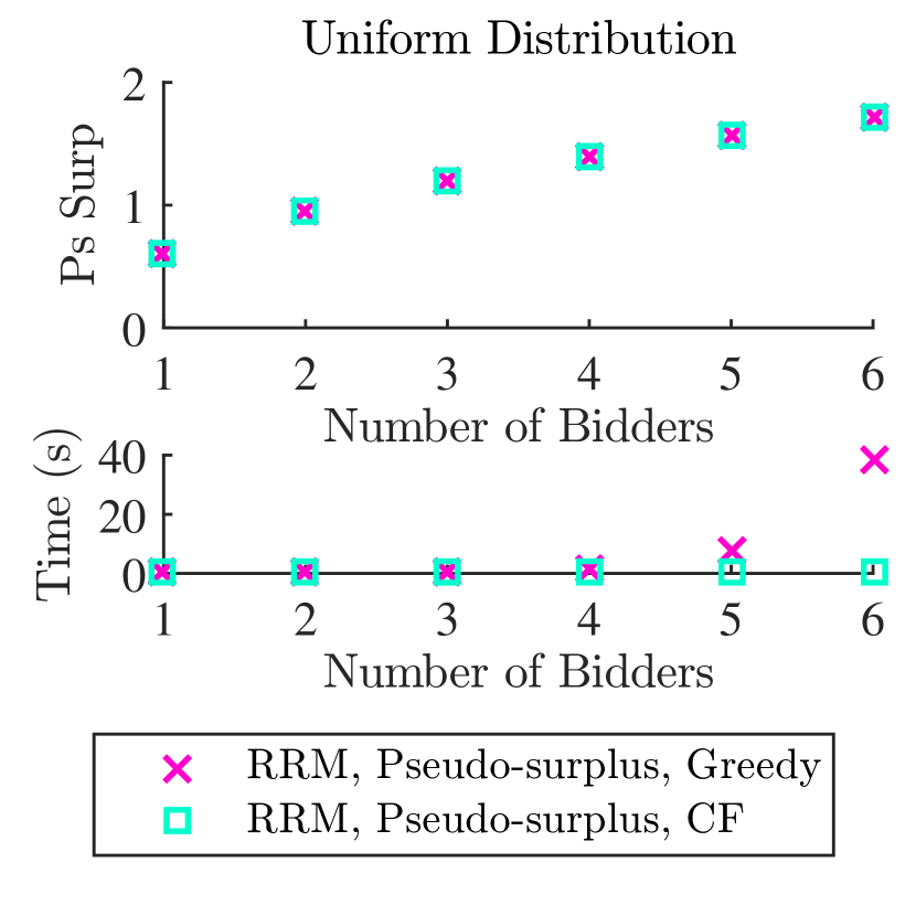
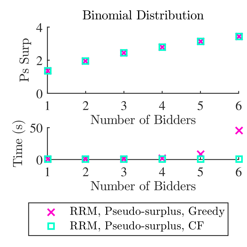
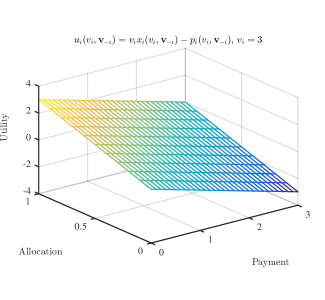
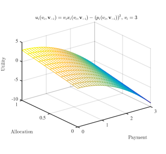
The shape of the utility function varies with the choice of qisubscript𝑞𝑖q_{i}: for example, it can be linear if we choose qisubscript𝑞𝑖q_{i} to be the identity function, or concave if we choose qi(pi(bi,𝐛i))=(pi(bi,𝐛i))2subscript𝑞𝑖subscript𝑝𝑖subscript𝑏𝑖subscript𝐛𝑖superscriptsubscript𝑝𝑖subscript𝑏𝑖subscript𝐛𝑖2q_{i}(p_{i}(b_{i},\mathbf{b}_{-i}))=(p_{i}(b_{i},\mathbf{b}_{-i}))^{2}. Figures 1 and 2 plot sample utility functions for these two choices of qisubscript𝑞𝑖q_{i}.

For readability, we usually write qi(bi,𝐛i)subscript𝑞𝑖subscript𝑏𝑖subscript𝐛𝑖q_{i}(b_{i},\mathbf{b}_{-i}) instead of qi(pi(bi,𝐛i))subscript𝑞𝑖subscript𝑝𝑖subscript𝑏𝑖subscript𝐛𝑖q_{i}(p_{i}(b_{i},\mathbf{b}_{-i})). Furthermore, we refer to the rule 𝐪(𝐛)n𝐪𝐛superscript𝑛\mathbf{q}(\mathbf{b})\in{\operatorname*{\mathbb{R}}}^{n} as the perceived payment rule, as these are payments the bidders impose upon themselves. Likewise, we think of 𝐩(𝐛)𝐩𝐛\mathbf{p}(\mathbf{b}) as an actual payment rule, as these are payments the bidders actually pay to the auctioneer. (But we usually omit the descriptor “actual,” as what it modifies is the actual payment rule!)

With this general utility function in mind, we proceed to formulate the optimal auction design problem: we seek the revenue-maximizing, ex-post feasible auction in which it is optimal for bidders to bid truthfully, and it is rational for them to participate. Once again, Myerson solved this problem in the quasi-linear case, assuming linear payments.
Refer to caption
Figure 1: Linear quasi-linear utility as a function of allocation and linear payments is shown, for ui(vi,𝐯i)=vixi(vi,𝐯i)pi(vi,𝐯i)subscript𝑢𝑖subscript𝑣𝑖subscript𝐯𝑖subscript𝑣𝑖subscript𝑥𝑖subscript𝑣𝑖subscript𝐯𝑖subscript𝑝𝑖subscript𝑣𝑖subscript𝐯𝑖u_{i}(v_{i},\mathbf{v}_{-i})=v_{i}x_{i}(v_{i},\mathbf{v}_{-i})-p_{i}(v_{i},\mathbf{v}_{-i}), where vi=3subscript𝑣𝑖3v_{i}=3. For a fixed allocation xi(vi,𝐯i)subscript𝑥𝑖subscript𝑣𝑖subscript𝐯𝑖x_{i}(v_{i},\mathbf{v}_{-i}), utility scales linearly with pi(vi,𝐯i)subscript𝑝𝑖subscript𝑣𝑖subscript𝐯𝑖p_{i}(v_{i},\mathbf{v}_{-i}), and for a fixed payment pi(vi,𝐯i)subscript𝑝𝑖subscript𝑣𝑖subscript𝐯𝑖p_{i}(v_{i},\mathbf{v}_{-i}), utility scales linearly with x(vi,𝐯i)𝑥subscript𝑣𝑖subscript𝐯𝑖x(v_{i},\mathbf{v}_{-i}). Utility is non-negative when vixi(vi,𝐯i)pi(vi,𝐯i)subscript𝑣𝑖subscript𝑥𝑖subscript𝑣𝑖subscript𝐯𝑖subscript𝑝𝑖subscript𝑣𝑖subscript𝐯𝑖v_{i}x_{i}(v_{i},\mathbf{v}_{-i})\geq p_{i}(v_{i},\mathbf{v}_{-i}), so individual rationality dictates that pi(vi,𝐯i)subscript𝑝𝑖subscript𝑣𝑖subscript𝐯𝑖p_{i}(v_{i},\mathbf{v}_{-i}) can be at most 333.
Refer to caption
Figure 2: Concave quasi-linear utility as a function of allocation and convex perceived payments is shown, for ui(vi,𝐯i)=vixi(vi,𝐯i)(pi(vi,𝐯i))2subscript𝑢𝑖subscript𝑣𝑖subscript𝐯𝑖subscript𝑣𝑖subscript𝑥𝑖subscript𝑣𝑖subscript𝐯𝑖superscriptsubscript𝑝𝑖subscript𝑣𝑖subscript𝐯𝑖2u_{i}(v_{i},\mathbf{v}_{-i})=v_{i}x_{i}(v_{i},\mathbf{v}_{-i})-\left(p_{i}(v_{i},\mathbf{v}_{-i})\right)^{2}, where vi=3subscript𝑣𝑖3v_{i}=3. For a fixed allocation xi(vi,𝐯i)subscript𝑥𝑖subscript𝑣𝑖subscript𝐯𝑖x_{i}(v_{i},\mathbf{v}_{-i}), utility scales quadratically with pi(vi,𝐯i)subscript𝑝𝑖subscript𝑣𝑖subscript𝐯𝑖p_{i}(v_{i},\mathbf{v}_{-i}), and for a fixed payment pi(vi,𝐯i)subscript𝑝𝑖subscript𝑣𝑖subscript𝐯𝑖p_{i}(v_{i},\mathbf{v}_{-i}), utility scales linearly with xi(vi,𝐯i)subscript𝑥𝑖subscript𝑣𝑖subscript𝐯𝑖x_{i}(v_{i},\mathbf{v}_{-i}). Utility is non-negative when vixi(vi,𝐯i)pi(vi,𝐯i)subscript𝑣𝑖subscript𝑥𝑖subscript𝑣𝑖subscript𝐯𝑖subscript𝑝𝑖subscript𝑣𝑖subscript𝐯𝑖\sqrt{v_{i}x_{i}(v_{i},\mathbf{v}_{-i})}\geq p_{i}(v_{i},\mathbf{v}_{-i}), so individual rationality dictates that pi(vi,𝐯i)subscript𝑝𝑖subscript𝑣𝑖subscript𝐯𝑖p_{i}(v_{i},\mathbf{v}_{-i}) can be at most 33\sqrt{3}.

2.1 Constraints

In this section, we formalize the constraints we will impose on an optimal auction design. Because we restrict our attention to incentive compatible auctions, where it is optimal to bid truthfully, we write qi(vi,𝐯i)subscript𝑞𝑖subscript𝑣𝑖subscript𝐯𝑖q_{i}(v_{i},\mathbf{v}_{-i}) instead of qi(bi,𝐛i)subscript𝑞𝑖subscript𝑏𝑖subscript𝐛𝑖q_{i}(b_{i},\mathbf{b}_{-i}). (As usual, the variables qi(vi,𝐯i)subscript𝑞𝑖subscript𝑣𝑖subscript𝐯𝑖q_{i}(v_{i},\mathbf{v}_{-i}) comprise the perceived payment rule 𝐪(𝐯)n𝐪𝐯superscript𝑛\mathbf{q}(\mathbf{v})\in\mathbb{R}^{n}.)

A mechanism is called incentive compatible (IC) if each bidder maximizes her utility by reporting bids bisubscript𝑏𝑖b_{i} that are equal to values visubscript𝑣𝑖v_{i}: iNfor-all𝑖𝑁\forall i\in N, vi,wiTifor-allsubscript𝑣𝑖subscript𝑤𝑖subscript𝑇𝑖\forall v_{i},w_{i}\in T_{i}, and 𝐯iTifor-allsubscript𝐯𝑖subscript𝑇𝑖\forall\mathbf{v}_{-i}\in T_{-i},

vixi(vi,𝐯i)qi(vi,𝐯i)vixi(wi,𝐯i)qi(wi,𝐯i).subscript𝑣𝑖subscript𝑥𝑖subscript𝑣𝑖subscript𝐯𝑖subscript𝑞𝑖subscript𝑣𝑖subscript𝐯𝑖subscript𝑣𝑖subscript𝑥𝑖subscript𝑤𝑖subscript𝐯𝑖subscript𝑞𝑖subscript𝑤𝑖subscript𝐯𝑖v_{i}x_{i}(v_{i},\mathbf{v}_{-i})-q_{i}(v_{i},\mathbf{v}_{-i})\geq v_{i}x_{i}(w_{i},\mathbf{v}_{-i})-q_{i}(w_{i},\mathbf{v}_{-i}). (2)

Individual rationality (IR) ensures that bidders have non-negative utilities: iNfor-all𝑖𝑁\forall i\in N, viTifor-allsubscript𝑣𝑖subscript𝑇𝑖\forall v_{i}\in T_{i}, and 𝐯iTifor-allsubscript𝐯𝑖subscript𝑇𝑖\forall\mathbf{v}_{-i}\in T_{-i},

vixi(vi,𝐯i)qi(vi,𝐯i)0.subscript𝑣𝑖subscript𝑥𝑖subscript𝑣𝑖subscript𝐯𝑖subscript𝑞𝑖subscript𝑣𝑖subscript𝐯𝑖0v_{i}x_{i}(v_{i},\mathbf{v}_{-i})-q_{i}(v_{i},\mathbf{v}_{-i})\geq 0. (3)

Next, we define IC and IR in expectation (with respect to Fisubscript𝐹𝑖F_{-i}). To do so, we introduce interim allocation and interim perceived payment variables, respectively: x^i(vi)x^i(vi,)=𝔼𝐯i[xi(vi,𝐯i)]subscript^𝑥𝑖subscript𝑣𝑖subscript^𝑥𝑖subscript𝑣𝑖subscript𝔼subscript𝐯𝑖subscript𝑥𝑖subscript𝑣𝑖subscript𝐯𝑖\hat{x}_{i}(v_{i})\equiv\hat{x}_{i}(v_{i},\cdot)=\operatorname*{\mathbb{E}}_{\mathbf{v}_{-i}}\left[x_{i}(v_{i},\mathbf{v}_{-i})\right] and q^i(vi)q^i(vi,)=𝔼𝐯i[qi(vi,𝐯i)]subscript^𝑞𝑖subscript𝑣𝑖subscript^𝑞𝑖subscript𝑣𝑖subscript𝔼subscript𝐯𝑖subscript𝑞𝑖subscript𝑣𝑖subscript𝐯𝑖\hat{q}_{i}(v_{i})\equiv\hat{q}_{i}(v_{i},\cdot)=\operatorname*{\mathbb{E}}_{\mathbf{v}_{-i}}\left[q_{i}(v_{i},\mathbf{v}_{-i})\right]. These variables comprise the interim allocation and perceived payment rules, 𝐱^(𝐯)[0,1]n^𝐱𝐯superscript01𝑛\hat{\mathbf{x}}(\mathbf{v})\in[0,1]^{n} and 𝐪^(𝐯)n^𝐪𝐯superscript𝑛\hat{\mathbf{q}}(\mathbf{v})\in\mathbb{R}^{n}.

We call a mechanism Bayesian incentive compatible (BIC) if utility is maximized by truthful reports in expectation: iNfor-all𝑖𝑁\forall i\in N and vi,wiTifor-allsubscript𝑣𝑖subscript𝑤𝑖subscript𝑇𝑖\forall v_{i},w_{i}\in T_{i},

vix^i(vi)q^i(vi)vix^i(wi)q^i(wi).subscript𝑣𝑖subscript^𝑥𝑖subscript𝑣𝑖subscript^𝑞𝑖subscript𝑣𝑖subscript𝑣𝑖subscript^𝑥𝑖subscript𝑤𝑖subscript^𝑞𝑖subscript𝑤𝑖v_{i}\hat{x}_{i}(v_{i})-\hat{q}_{i}(v_{i})\geq v_{i}\hat{x}_{i}(w_{i})-\hat{q}_{i}(w_{i}). (4)

Bayesian individual rationality (BIR) insists on non-negative utilities in expectation: iNfor-all𝑖𝑁\forall i\in N and viTifor-allsubscript𝑣𝑖subscript𝑇𝑖\forall v_{i}\in T_{i},

vix^i(vi)q^i(vi)0.subscript𝑣𝑖subscript^𝑥𝑖subscript𝑣𝑖subscript^𝑞𝑖subscript𝑣𝑖0v_{i}\hat{x}_{i}(v_{i})-\hat{q}_{i}(v_{i})\geq 0. (5)

We say a mechanism is ex-post feasible (XP) if it never overallocates: 𝐯Tfor-all𝐯𝑇\forall\mathbf{v}\in T,

i=1nxi(vi,𝐯i)1.superscriptsubscript𝑖1𝑛subscript𝑥𝑖subscript𝑣𝑖subscript𝐯𝑖1\sum_{i=1}^{n}x_{i}(v_{i},\mathbf{v}_{-i})\leq 1. (6)

Ex-ante feasibility (XA) is satisfied if, in expectation, the mechanism does not over-allocate:

𝔼𝐯[i=1nxi(𝐯)]1.subscript𝔼𝐯superscriptsubscript𝑖1𝑛subscript𝑥𝑖𝐯1\operatorname*{\mathbb{E}}_{\mathbf{v}}\left[\sum_{i=1}^{n}x_{i}(\mathbf{v})\right]\leq 1. (7)

Finally, we require that 0xi(vi,𝐯i),x^i(vi)1formulae-sequence0subscript𝑥𝑖subscript𝑣𝑖subscript𝐯𝑖subscript^𝑥𝑖subscript𝑣𝑖10\leq x_{i}(v_{i},\mathbf{v}_{-i}),\hat{x}_{i}(v_{i})\leq 1, iNfor-all𝑖𝑁\forall i\in N, viTifor-allsubscript𝑣𝑖subscript𝑇𝑖\forall v_{i}\in T_{i} and 𝐯iTifor-allsubscript𝐯𝑖subscript𝑇𝑖\forall\mathbf{v}_{-i}\in T_{-i}.

2.2 Revenue Maximization

The robust revenue-maximization problem (RRM) is to maximize total expected payments (i.e., 𝔼𝐯[i=1npi(vi,𝐯i)]subscript𝔼𝐯superscriptsubscript𝑖1𝑛subscript𝑝𝑖subscript𝑣𝑖subscript𝐯𝑖\operatorname*{\mathbb{E}}_{\mathbf{v}}\left[\sum_{i=1}^{n}p_{i}(v_{i},\mathbf{v}_{-i})\right]), subject to IR, IC, and ex-post feasibility. RRM is expressed as a mathematical program in Section C.1.1. A typical relaxation of this problem insists on ex-ante feasibility only.

Likewise, the Bayesian revenue-maximization problem (BRM) is to maximize total expected payments subject to BIR, BIC, and ex-post feasibility (or ex-ante feasibility). BRM with ex-post feasibility is expressed as a mathematical program in Section C.2.1. BRM with ex-ante feasibility is expressed as a mathematical program in Section C.3.1.

In both RRM and BRM, there are exponentially-many ex-post feasibility constraints, and exponentially-many allocation and payment variables. However, revenue maximization subject to BIC and BIR but only ex-ante feasibility involves only one feasibility constraint and polynomially-many interim allocation and payment variables.

In this paper, we assume qi(pi(vi,𝐯i))=(pi(vi,𝐯i))2subscript𝑞𝑖subscript𝑝𝑖subscript𝑣𝑖subscript𝐯𝑖superscriptsubscript𝑝𝑖subscript𝑣𝑖subscript𝐯𝑖2q_{i}(p_{i}(v_{i},\mathbf{v}_{-i}))=(p_{i}(v_{i},\mathbf{v}_{-i}))^{2} (or qi=pi2subscript𝑞𝑖superscriptsubscript𝑝𝑖2q_{i}=p_{i}^{2}, for short). This choice of perceived payments yields quadratic constraints. While small instances of the quadratic programs that express BRM and RRM can be solved by standard mathematical programming solvers, this approach does not scale. We are interested in finding scalable algorithms that produce approximately-optimal solutions to these problems.

3 Myerson’s Payment Formula

We start by providing a straightforward adaptation of Myerson’s payment formula [8] to the case where the utilities are of the concave form of interest.

For consistency with our implementations,222True to our profession—computer science—we have implemented all mechanisms discussed in this paper. we describe our contributions under the assumption that type distributions are discrete, but our theoretical results are in no way contingent on this assumption. Specifically, we assume the distribution of values is drawn from the discrete type space Ti={zi,k:1kMi}subscript𝑇𝑖conditional-setsubscript𝑧𝑖𝑘1𝑘subscript𝑀𝑖T_{i}=\{z_{i,k}:1\leq k\leq M_{i}\}, of cardinality Misubscript𝑀𝑖M_{i}, where zi,j<zi,ksubscript𝑧𝑖𝑗subscript𝑧𝑖𝑘z_{i,j}<z_{i,k} for j<k𝑗𝑘j<k, and we let zi,Mi+1=zi,Misubscript𝑧𝑖subscript𝑀𝑖1subscript𝑧𝑖subscript𝑀𝑖z_{i,{M_{i}}+1}=z_{i,{M_{i}}}. Furthermore, let fi(vi)subscript𝑓𝑖subscript𝑣𝑖f_{i}(v_{i}) be the probability of viTisubscript𝑣𝑖subscript𝑇𝑖v_{i}\in T_{i}, let f(𝐯)𝑓𝐯f(\mathbf{v}) be the probability of 𝐯T𝐯𝑇\mathbf{v}\in T, and let fi(𝐯i)subscript𝑓𝑖subscript𝐯𝑖f_{-i}(\mathbf{v}_{-i}) be the probability of 𝐯iTisubscript𝐯𝑖subscript𝑇𝑖\mathbf{v}_{-i}\in T_{-i}.

Myerson’s payment theorem, which takes as a starting point the bidders’ utility functions (i.e., Equation (1)), applies immediately to the perceived payment rules 𝐪𝐪\mathbf{q} and 𝐪^^𝐪\hat{\mathbf{q}}:

Theorem 3.1.

Assume bidders’ utilities take the form of Equation (1). A mechanism is IC and IR iff for each bidder iN𝑖𝑁i\in N:

  • the allocation rule 𝐱𝐱\mathbf{x} is monotone, i.e., viwiTifor-allsubscript𝑣𝑖subscript𝑤𝑖subscript𝑇𝑖\forall v_{i}\geq w_{i}\in T_{i} and 𝐯iTifor-allsubscript𝐯𝑖subscript𝑇𝑖\forall\mathbf{v}_{-i}\in T_{-i}, xi(vi,𝐯i)xi(wi,𝐯i)subscript𝑥𝑖subscript𝑣𝑖subscript𝐯𝑖subscript𝑥𝑖subscript𝑤𝑖subscript𝐯𝑖x_{i}(v_{i},\mathbf{v}_{-i})\geq x_{i}(w_{i},\mathbf{v}_{-i}); and

  • the perceived payment rule 𝐪𝐪\mathbf{q} is given by: zi,Tifor-allsubscript𝑧𝑖subscript𝑇𝑖\forall z_{i,\ell}\in T_{i} and 𝐯iTifor-allsubscript𝐯𝑖subscript𝑇𝑖\forall\mathbf{v}_{-i}\in T_{-i},

    qi(zi,,𝐯i)=zi,xi(zi,,𝐯i)j=11(zi,j+1zi,j)xi(zi,j,𝐯i)subscript𝑞𝑖subscript𝑧𝑖subscript𝐯𝑖subscript𝑧𝑖subscript𝑥𝑖subscript𝑧𝑖subscript𝐯𝑖superscriptsubscript𝑗11subscript𝑧𝑖𝑗1subscript𝑧𝑖𝑗subscript𝑥𝑖subscript𝑧𝑖𝑗subscript𝐯𝑖q_{i}(z_{i,\ell},\mathbf{v}_{-i})=z_{i,\ell}x_{i}(z_{i,\ell},\mathbf{v}_{-i})-\sum_{j=1}^{\ell-1}(z_{i,j+1}-z_{i,j})x_{i}(z_{i,j},\mathbf{v}_{-i}) (8)

    where qi(0,𝐯i)=0subscript𝑞𝑖0subscript𝐯𝑖0q_{i}(0,\mathbf{v}_{-i})=0.

Likewise, in the Bayesian setting, a mechanism is BIC and BIR iff for each bidder iN𝑖𝑁i\in N:

  • the allocation rule 𝐱^^𝐱\hat{\mathbf{x}} is monotone, i.e., viwiTifor-allsubscript𝑣𝑖subscript𝑤𝑖subscript𝑇𝑖\forall v_{i}\geq w_{i}\in T_{i}, x^i(vi)x^i(wi)subscript^𝑥𝑖subscript𝑣𝑖subscript^𝑥𝑖subscript𝑤𝑖\hat{x}_{i}(v_{i})\geq\hat{x}_{i}(w_{i}); and

  • the perceived payment rule 𝐪^^𝐪\hat{\mathbf{q}} is given by: zi,Tifor-allsubscript𝑧𝑖subscript𝑇𝑖\forall z_{i,\ell}\in T_{i},

    q^i(zi,)=zi,x^i(zi,)j=11(zi,j+1zi,j)x^i(zi,j)subscript^𝑞𝑖subscript𝑧𝑖subscript𝑧𝑖subscript^𝑥𝑖subscript𝑧𝑖superscriptsubscript𝑗11subscript𝑧𝑖𝑗1subscript𝑧𝑖𝑗subscript^𝑥𝑖subscript𝑧𝑖𝑗\hat{q}_{i}(z_{i,\ell})=z_{i,\ell}\hat{x}_{i}(z_{i,\ell})-\sum_{j=1}^{\ell-1}(z_{i,j+1}-z_{i,j})\hat{x}_{i}(z_{i,j}) (9)

    where q^i(0)=0subscript^𝑞𝑖00\hat{q}_{i}(0)=0.

Remark 3.2.

The monotonicity of the allocation rule ensures that the perceived payment rule is also monotonic. Specifically, the perceived payment associated with a bidder of type zi,+1subscript𝑧𝑖1z_{i,\ell+1} is at least as great as the perceived payment associated with a bidder of type zi,subscript𝑧𝑖z_{i,\ell}:

qi(zi,+1,𝐯i)subscript𝑞𝑖subscript𝑧𝑖1subscript𝐯𝑖\displaystyle q_{i}(z_{i,\ell+1},\mathbf{v}_{-i}) =zi,+1xi(zi,+1,𝐯i)j=1(zi,j+1zi,j)xi(zi,j,𝐯i)absentsubscript𝑧𝑖1subscript𝑥𝑖subscript𝑧𝑖1subscript𝐯𝑖superscriptsubscript𝑗1subscript𝑧𝑖𝑗1subscript𝑧𝑖𝑗subscript𝑥𝑖subscript𝑧𝑖𝑗subscript𝐯𝑖\displaystyle=z_{i,\ell+1}x_{i}(z_{i,\ell+1},\mathbf{v}_{-i})-\sum_{j=1}^{\ell}\left(z_{i,j+1}-z_{i,j}\right)x_{i}(z_{i,j},\mathbf{v}_{-i})
=zi,+1(xi(zi,+1,𝐯i)xi(zi,,𝐯i))+zi,xi(zi,,𝐯i)j=11(zi,j+1zi,j)xi(zi,j,𝐯i)absentsubscript𝑧𝑖1subscript𝑥𝑖subscript𝑧𝑖1subscript𝐯𝑖subscript𝑥𝑖subscript𝑧𝑖subscript𝐯𝑖subscript𝑧𝑖subscript𝑥𝑖subscript𝑧𝑖subscript𝐯𝑖superscriptsubscript𝑗11subscript𝑧𝑖𝑗1subscript𝑧𝑖𝑗subscript𝑥𝑖subscript𝑧𝑖𝑗subscript𝐯𝑖\displaystyle=z_{i,\ell+1}\left(x_{i}(z_{i,\ell+1},\mathbf{v}_{-i})-x_{i}(z_{i,\ell},\mathbf{v}_{-i})\right)+z_{i,\ell}x_{i}(z_{i,\ell},\mathbf{v}_{-i})-\sum_{j=1}^{\ell-1}(z_{i,j+1}-z_{i,j})x_{i}(z_{i,j},\mathbf{v}_{-i})
=zi,+1(xi(zi,+1,𝐯i)xi(zi,,𝐯i))+qi(zi,,𝐯i)absentsubscript𝑧𝑖1subscript𝑥𝑖subscript𝑧𝑖1subscript𝐯𝑖subscript𝑥𝑖subscript𝑧𝑖subscript𝐯𝑖subscript𝑞𝑖subscript𝑧𝑖subscript𝐯𝑖\displaystyle=z_{i,\ell+1}\left(x_{i}(z_{i,\ell+1},\mathbf{v}_{-i})-x_{i}(z_{i,\ell},\mathbf{v}_{-i})\right)+q_{i}(z_{i,\ell},\mathbf{v}_{-i})
qi(zi,,𝐯i).absentsubscript𝑞𝑖subscript𝑧𝑖subscript𝐯𝑖\displaystyle\geq q_{i}(z_{i,\ell},\mathbf{v}_{-i}).

But as our goal is to maximize revenue, we are interested not in the bidders’ perceived payments, but rather in the actual payments to the auctioneer, namely 𝐩(𝐯),𝐩^(𝐯)n𝐩𝐯^𝐩𝐯superscript𝑛\mathbf{p}(\mathbf{v}),\hat{\mathbf{p}}(\mathbf{v})\in\mathbb{R}^{n}, the latter of which is comprised of variables p^i(vi)p^i(vi,)=𝔼𝐯i[pi(vi,𝐯i)]subscript^𝑝𝑖subscript𝑣𝑖subscript^𝑝𝑖subscript𝑣𝑖subscript𝔼subscript𝐯𝑖subscript𝑝𝑖subscript𝑣𝑖subscript𝐯𝑖\hat{p}_{i}(v_{i})\equiv\hat{p}_{i}(v_{i},\cdot)=\operatorname*{\mathbb{E}}_{\mathbf{v}_{-i}}\left[p_{i}(v_{i},\mathbf{v}_{-i})\right]. In the robust problem, the generalization is straightforward: since qi(zi,,𝐯i)=(pi(zi,,𝐯i))2subscript𝑞𝑖subscript𝑧𝑖subscript𝐯𝑖superscriptsubscript𝑝𝑖subscript𝑧𝑖subscript𝐯𝑖2q_{i}(z_{i,\ell},\mathbf{v}_{-i})=(p_{i}(z_{i,\ell},\mathbf{v}_{-i}))^{2}, it follows that pi(zi,,𝐯i)subscript𝑝𝑖subscript𝑧𝑖subscript𝐯𝑖p_{i}(z_{i,\ell},\mathbf{v}_{-i}) is simply the square root of qi(zi,,𝐯i)subscript𝑞𝑖subscript𝑧𝑖subscript𝐯𝑖q_{i}(z_{i,\ell},\mathbf{v}_{-i}).

In the Bayesian problem, however, q^i(zi,)subscript^𝑞𝑖subscript𝑧𝑖\hat{q}_{i}(z_{i,\ell}) need not equal (p^i(zi,))2superscriptsubscript^𝑝𝑖subscript𝑧𝑖2(\hat{p}_{i}(z_{i,\ell}))^{2}, because q^i(zi,)=𝔼𝐯i[qi(zi,,𝐯i)]=𝔼𝐯i[(pi(zi,,𝐯i))2](𝔼𝐯i[pi(zi,,𝐯i)])2(p^i(zi,))2subscript^𝑞𝑖subscript𝑧𝑖subscript𝔼subscript𝐯𝑖subscript𝑞𝑖subscript𝑧𝑖subscript𝐯𝑖subscript𝔼subscript𝐯𝑖superscriptsubscript𝑝𝑖subscript𝑧𝑖subscript𝐯𝑖2superscriptsubscript𝔼subscript𝐯𝑖subscript𝑝𝑖subscript𝑧𝑖subscript𝐯𝑖2superscriptsubscript^𝑝𝑖subscript𝑧𝑖2\hat{q}_{i}(z_{i,\ell})=\operatorname*{\mathbb{E}}_{\mathbf{v}_{-i}}\left[q_{i}(z_{i,\ell},\mathbf{v}_{-i})\right]=\operatorname*{\mathbb{E}}_{\mathbf{v}_{-i}}\left[(p_{i}(z_{i,\ell},\mathbf{v}_{-i}))^{2}\right]\neq\left(\operatorname*{\mathbb{E}}_{\mathbf{v}_{-i}}\left[p_{i}(z_{i,\ell},\mathbf{v}_{-i})\right]\right)^{2}\equiv(\hat{p}_{i}(z_{i,\ell}))^{2}. Nonetheless, in Section 6, we successfully derive an interim payment function hi(zi,)subscript𝑖subscript𝑧𝑖h_{i}(z_{i,\ell}) for which q^i(zi,)=(hi(zi,))2subscript^𝑞𝑖subscript𝑧𝑖superscriptsubscript𝑖subscript𝑧𝑖2\hat{q}_{i}(z_{i,\ell})=(h_{i}(z_{i,\ell}))^{2}, so that hi(zi,)subscript𝑖subscript𝑧𝑖h_{i}(z_{i,\ell}) is the square root of q^i(zi,)subscript^𝑞𝑖subscript𝑧𝑖\hat{q}_{i}(z_{i,\ell}).333In Algorithms 7) and 10, the payment rule 𝐡(𝐯)n𝐡𝐯superscript𝑛\mathbf{h}(\mathbf{v})\in\mathbb{R}^{n}, is comprised of variables hi(vi)subscript𝑖subscript𝑣𝑖h_{i}(v_{i}).

Corollary 3.3.

Under the assumptions of Theorem 3.1, for qi(zi,,𝐯i)=(pi(zi,,𝐯i))2subscript𝑞𝑖subscript𝑧𝑖subscript𝐯𝑖superscriptsubscript𝑝𝑖subscript𝑧𝑖subscript𝐯𝑖2q_{i}(z_{i,\ell},\mathbf{v}_{-i})=(p_{i}(z_{i,\ell},\mathbf{v}_{-i}))^{2},

pi(zi,,𝐯i)=zi,xi(zi,,𝐯i)j=11(zi,j+1zi,j)xi(zij,𝐯i).subscript𝑝𝑖subscript𝑧𝑖subscript𝐯𝑖subscript𝑧𝑖subscript𝑥𝑖subscript𝑧𝑖subscript𝐯𝑖superscriptsubscript𝑗11subscript𝑧𝑖𝑗1subscript𝑧𝑖𝑗subscript𝑥𝑖subscript𝑧𝑖𝑗subscript𝐯𝑖p_{i}(z_{i,\ell},\mathbf{v}_{-i})=\sqrt{z_{i,\ell}x_{i}(z_{i,\ell},\mathbf{v}_{-i})-\sum_{j=1}^{\ell-1}(z_{i,j+1}-z_{i,j})x_{i}(z_{ij},\mathbf{v}_{-i})}. (10)

Likewise, given an interim payment function hi:Ti:subscript𝑖subscript𝑇𝑖h_{i}:T_{i}\to\operatorname*{\mathbb{R}} such that q^i(zi,)=(hi(zi,))2subscript^𝑞𝑖subscript𝑧𝑖superscriptsubscript𝑖subscript𝑧𝑖2\hat{q}_{i}(z_{i,\ell})=(h_{i}(z_{i,\ell}))^{2}, then

hi(zi,)=zi,x^i(zi,)j=11(zi,j+1zi,j)x^i(zi,j).subscript𝑖subscript𝑧𝑖subscript𝑧𝑖subscript^𝑥𝑖subscript𝑧𝑖superscriptsubscript𝑗11subscript𝑧𝑖𝑗1subscript𝑧𝑖𝑗subscript^𝑥𝑖subscript𝑧𝑖𝑗h_{i}(z_{i,\ell})=\sqrt{z_{i,\ell}\hat{x}_{i}(z_{i,\ell})-\sum_{j=1}^{\ell-1}(z_{i,j+1}-z_{i,j})\hat{x}_{i}(z_{i,j})}. (11)

Myerson’s payment formula is immensely powerful. It gives rise to a procedure for optimal auction design that at first glance borders on the miraculous. The procedure is thus: First, solve for an allocation rule that optimizes your objective (surplus, revenue, what have you), subject only to ex-post feasibility. Second, check for monotonicity. If the optimal allocation rule is indeed monotonic, then you are home free; you need only plug that allocation rule into Myerson’s payment formula and you will have imposed incentive compatibility and individual rationality without sacrificing one ounce of optimality!. In other words, given a monotone allocation rule, IC and IR are yours for the taking. That is the essence of Myerson’s approach, and something we exploit heavily in this work.

4 Robust vs. Bayesian Optimal Auctions

Another of the more surprising facts that Myerson discovered about the optimal auction design problem (assuming linear perceived payments) is that the total expected revenue in the robust and Bayesian problems are equivalent. It is clear that the value of a solution to BRM must be at least that of RRM, since the objectives are the same while BRM’s constraints are weaker. It is the other direction, namely that the value of a solution to BRM never exceeds that of RRM, which is surprising. This latter relies on the assumption that perceived payments, and hence utilities, are linear, and therefore does not hold in our setting with convex perceived payments, and hence concave utilities, which we now proceed to show via counterexample.

4.1 Robust Revenue \neq Bayesian Revenue

We begin our analysis of BRM vs. RRM with convex perceived payments by demonstrating via example that solutions to BRM can strictly exceed those of RRM when qi=pi2subscript𝑞𝑖superscriptsubscript𝑝𝑖2q_{i}=p_{i}^{2}. Therefore, an optimal solution to RRM does not generally yield an optimal solution to BRM, although it does yield an immediate lower bound.

Example 4.1.

Suppose we have n=2𝑛2n=2 symmetric bidders, where for each bidder iN={1,2}𝑖𝑁12i\in N=\{1,2\}, Ti={0,100}subscript𝑇𝑖0100T_{i}=\{0,100\}, and for each value viTisubscript𝑣𝑖subscript𝑇𝑖v_{i}\in T_{i}, fi(vi)=1/2subscript𝑓𝑖subscript𝑣𝑖12f_{i}(v_{i})=1/2.

RRM

Our goal is to maximize revenue, while satisfying IC, IR, and the ex-post feasibility constraints. This mathematical program appears in Section C.1.1.

We know from IR that qi(vi,𝐯i)subscript𝑞𝑖subscript𝑣𝑖subscript𝐯𝑖q_{i}(v_{i},\mathbf{v}_{-i}) is upper-bounded by vixi(vi,𝐯i)subscript𝑣𝑖subscript𝑥𝑖subscript𝑣𝑖subscript𝐯𝑖v_{i}x_{i}(v_{i},\mathbf{v}_{-i}). So when vi=0subscript𝑣𝑖0v_{i}=0, qi(vi,𝐯i)0subscript𝑞𝑖subscript𝑣𝑖subscript𝐯𝑖0q_{i}(v_{i},\mathbf{v}_{-i})\leq 0. So we can set xi(vi,𝐯i)=0subscript𝑥𝑖subscript𝑣𝑖subscript𝐯𝑖0x_{i}(v_{i},\mathbf{v}_{-i})=0, for all 𝐯iTisubscript𝐯𝑖subscript𝑇𝑖\mathbf{v}_{-i}\in T_{-i}.

When one bidder, say i𝑖i, has type 100100100, and the other bidder has type 00, we maximize total payments by setting xi(100,0)=1subscript𝑥𝑖10001x_{i}(100,0)=1.

When both bidders have type 100100100, by Equation (10), pi(100,100)=100xi(100,100)subscript𝑝𝑖100100100subscript𝑥𝑖100100p_{i}(100,100)=\sqrt{100\,x_{i}(100,100)}. Therefore, total payments are maximized when xi(100,100)=1/2subscript𝑥𝑖10010012x_{i}(100,100)=1/2.

Thus, in the robust problem, the following allocation is optimal:

x1(0,0)subscript𝑥100\displaystyle x_{1}(0,0) =0absent0\displaystyle=0 x2(0,0)subscript𝑥200\displaystyle\quad x_{2}(0,0) =0absent0\displaystyle=0
x1(100,0)subscript𝑥11000\displaystyle x_{1}(100,0) =1absent1\displaystyle=1 x2(100,0)subscript𝑥21000\displaystyle\quad x_{2}(100,0) =0absent0\displaystyle=0
x1(0,100)subscript𝑥10100\displaystyle x_{1}(0,100) =0absent0\displaystyle=0 x2(0,100)subscript𝑥20100\displaystyle\quad x_{2}(0,100) =1absent1\displaystyle=1
x1(100,100)subscript𝑥1100100\displaystyle x_{1}(100,100) =1/2absent12\displaystyle=1/2 x2(100,100)subscript𝑥2100100\displaystyle\quad x_{2}(100,100) =1/2.absent12\displaystyle=1/2.

Computing payments according to Equation (10) yields:

p1(0,0)subscript𝑝100\displaystyle p_{1}(0,0) =0absent0\displaystyle=0 p2(0,0)subscript𝑝200\displaystyle\quad p_{2}(0,0) =0absent0\displaystyle=0
p1(100,0)subscript𝑝11000\displaystyle p_{1}(100,0) =10absent10\displaystyle=10 p2(100,0)subscript𝑝21000\displaystyle\quad p_{2}(100,0) =0absent0\displaystyle=0
p1(0,100)subscript𝑝10100\displaystyle p_{1}(0,100) =0absent0\displaystyle=0 p2(0,100)subscript𝑝20100\displaystyle\quad p_{2}(0,100) =10absent10\displaystyle=10
p1(100,100)subscript𝑝1100100\displaystyle p_{1}(100,100) =50absent50\displaystyle=\sqrt{50} p2(100,100)subscript𝑝2100100\displaystyle\quad p_{2}(100,100) =50.absent50\displaystyle=\sqrt{50}.

Therefore, the total expected revenue in the robust problem is:

i=1n𝐯f(𝐯)pi(vi,𝐯i)superscriptsubscript𝑖1𝑛subscript𝐯𝑓𝐯subscript𝑝𝑖subscript𝑣𝑖subscript𝐯𝑖\displaystyle\sum_{i=1}^{n}\sum_{\mathbf{v}}f(\mathbf{v})p_{i}(v_{i},\mathbf{v}_{-i}) =2𝐯f(𝐯)pi(vi,𝐯i)absent2subscript𝐯𝑓𝐯subscript𝑝𝑖subscript𝑣𝑖subscript𝐯𝑖\displaystyle=2\sum_{\mathbf{v}}f(\mathbf{v})p_{i}(v_{i},\mathbf{v}_{-i})
=2(14(0+10+0+50))absent214010050\displaystyle=2\left(\frac{1}{4}\left(0+10+0+\sqrt{50}\right)\right)
=5(1+22).absent5122\displaystyle=5\left(1+\frac{\sqrt{2}}{2}\right).
BRM

Our goal is to maximize revenue, while satisfying BIC, BIR and the ex-post feasibility constraints. This mathematical program appears in Section C.2.1.

We know from BIR that q^i(vi)subscript^𝑞𝑖subscript𝑣𝑖\hat{q}_{i}(v_{i}) is upper-bounded by vix^i(vi)subscript𝑣𝑖subscript^𝑥𝑖subscript𝑣𝑖v_{i}\hat{x}_{i}(v_{i}). So when vi=0subscript𝑣𝑖0v_{i}=0, q^i(vi)0subscript^𝑞𝑖subscript𝑣𝑖0\hat{q}_{i}(v_{i})\leq 0. So we can set x^i(vi)=0subscript^𝑥𝑖subscript𝑣𝑖0\hat{x}_{i}(v_{i})=0, which implies that xi(0,𝐯i)=0subscript𝑥𝑖0subscript𝐯𝑖0x_{i}(0,\mathbf{v}_{-i})=0, for all 𝐯iTisubscript𝐯𝑖subscript𝑇𝑖\mathbf{v}_{-i}\in T_{-i}. Additionally, since q^i(0)=𝔼𝐯i[(pi(0,𝐯i))2]subscript^𝑞𝑖0subscript𝔼subscript𝐯𝑖superscriptsubscript𝑝𝑖0subscript𝐯𝑖2\hat{q}_{i}(0)=\operatorname*{\mathbb{E}}_{\mathbf{v}_{-i}}\left[\left(p_{i}(0,\mathbf{v}_{-i})\right)^{2}\right], this also means that pi(0,𝐯i)=0subscript𝑝𝑖0subscript𝐯𝑖0p_{i}(0,\mathbf{v}_{-i})=0, for all 𝐯iTisubscript𝐯𝑖subscript𝑇𝑖\mathbf{v}_{-i}\in T_{-i}.

When vi=100subscript𝑣𝑖100v_{i}=100, we want to maximize x^i(vi)subscript^𝑥𝑖subscript𝑣𝑖\hat{x}_{i}(v_{i}) so that we can maximize q^i(vi)subscript^𝑞𝑖subscript𝑣𝑖\hat{q}_{i}(v_{i}), as this will maximize the payments the auctioneer collects when a bidder has type 100100100. For bidder 1:

x^1(100)subscript^𝑥1100\displaystyle\hat{x}_{1}(100) =f1(0)x1(100,0)+f1(100)x1(100,100)absentsubscript𝑓10subscript𝑥11000subscript𝑓1100subscript𝑥1100100\displaystyle=f_{-1}(0)x_{1}(100,0)+f_{-1}(100)x_{1}(100,100)
=12(x1(100,0)+x1(100,100)).absent12subscript𝑥11000subscript𝑥1100100\displaystyle=\frac{1}{2}\left(x_{1}(100,0)+x_{1}(100,100)\right).

We can set x1(100,0)subscript𝑥11000x_{1}(100,0) to 111, which leaves only x1(100,100)subscript𝑥1100100x_{1}(100,100) to be determined. Since the setting is symmetric, we can also set x2(0,100)=1subscript𝑥201001x_{2}(0,100)=1, leaving x2(100,100)subscript𝑥2100100x_{2}(100,100) also to be determined.

Rewriting the BIR constraints using payment terms explicitly, we have

100(12x1(100,0)+12x1(100,100))12((p1(100,0))2+(p1(100,100))2)10012subscript𝑥1100012subscript𝑥110010012superscriptsubscript𝑝110002superscriptsubscript𝑝11001002\displaystyle 100\left(\frac{1}{2}x_{1}(100,0)+\frac{1}{2}x_{1}(100,100)\right)\geq\frac{1}{2}\left(\left(p_{1}(100,0)\right)^{2}+\left(p_{1}(100,100)\right)^{2}\right)
100(12x2(0,100)+12x2(100,100))12((p2(0,100))2+(p2(100,100))2)10012subscript𝑥2010012subscript𝑥210010012superscriptsubscript𝑝201002superscriptsubscript𝑝21001002\displaystyle 100\left(\frac{1}{2}x_{2}(0,100)+\frac{1}{2}x_{2}(100,100)\right)\geq\frac{1}{2}\left(\left(p_{2}(0,100)\right)^{2}+\left(p_{2}(100,100)\right)^{2}\right)

Equivalently,

100(12+12x1(100,100))12((p1(100,0))2+(p1(100,100))2)1001212subscript𝑥110010012superscriptsubscript𝑝110002superscriptsubscript𝑝11001002\displaystyle 100\left(\frac{1}{2}+\frac{1}{2}x_{1}(100,100)\right)\geq\frac{1}{2}\left(\left(p_{1}(100,0)\right)^{2}+\left(p_{1}(100,100)\right)^{2}\right)
100(12+12(1x1(100,100)))12((p2(0,100))2+(p2(100,100))2)10012121subscript𝑥110010012superscriptsubscript𝑝201002superscriptsubscript𝑝21001002\displaystyle 100\left(\frac{1}{2}+\frac{1}{2}\left(1-x_{1}(100,100)\right)\right)\geq\frac{1}{2}\left(\left(p_{2}(0,100)\right)^{2}+\left(p_{2}(100,100)\right)^{2}\right)

Combining the inequalities yields

15012((p1(100,0))2+(p1(100,100))2+(p2(0,100))2+(p2(100,100))2)15012superscriptsubscript𝑝110002superscriptsubscript𝑝11001002superscriptsubscript𝑝201002superscriptsubscript𝑝21001002150\geq\frac{1}{2}\bigg{(}\left(p_{1}(100,0)\right)^{2}+\left(p_{1}(100,100)\right)^{2}+\left(p_{2}(0,100)\right)^{2}+\left(p_{2}(100,100)\right)^{2}\bigg{)}

Subject to this constraint, we can maximize total payments,

p1(100,0)+p1(100,100)+p2(0,100)+p2(100,100),subscript𝑝11000subscript𝑝1100100subscript𝑝20100subscript𝑝2100100\displaystyle p_{1}(100,0)+p_{1}(100,100)+p_{2}(0,100)+p_{2}(100,100),

by equating each of the four payment terms, so that pi(100,𝐯i)=53subscript𝑝𝑖100subscript𝐯𝑖53p_{i}(100,\mathbf{v}_{-i})=5\sqrt{3}.

In summary, the following payment rule maximizes revenue:

pi(0,𝐯i)subscript𝑝𝑖0subscript𝐯𝑖\displaystyle p_{i}(0,\mathbf{v}_{-i}) =0,absent0\displaystyle=0, iN,𝐯iTiformulae-sequencefor-all𝑖𝑁for-allsubscript𝐯𝑖subscript𝑇𝑖\displaystyle\forall i\in N,\forall\mathbf{v}_{-i}\in T_{-i}
pi(100,𝐯i)subscript𝑝𝑖100subscript𝐯𝑖\displaystyle p_{i}(100,\mathbf{v}_{-i}) =53,absent53\displaystyle=5\sqrt{3}, iN,𝐯iTi.formulae-sequencefor-all𝑖𝑁for-allsubscript𝐯𝑖subscript𝑇𝑖\displaystyle\forall i\in N,\forall\mathbf{v}_{-i}\in T_{-i}.

This payment rule implies a symmetric allocation in which x1(100,0)=x2(0,100)=12subscript𝑥11000subscript𝑥2010012x_{1}(100,0)=x_{2}(0,100)=\frac{1}{2}. Therefore, this BRM problem can be solved using the same allocation rule as the corresponding RRM problem:

x1(0,0)subscript𝑥100\displaystyle x_{1}(0,0) =0absent0\displaystyle=0 x2(0,0)subscript𝑥200\displaystyle\quad x_{2}(0,0) =0absent0\displaystyle=0
x1(100,0)subscript𝑥11000\displaystyle x_{1}(100,0) =1absent1\displaystyle=1 x2(100,0)subscript𝑥21000\displaystyle\quad x_{2}(100,0) =0absent0\displaystyle=0
x1(0,100)subscript𝑥10100\displaystyle x_{1}(0,100) =0absent0\displaystyle=0 x2(0,100)subscript𝑥20100\displaystyle\quad x_{2}(0,100) =1absent1\displaystyle=1
x1(100,100)subscript𝑥1100100\displaystyle x_{1}(100,100) =1/2absent12\displaystyle=1/2 x2(100,100)subscript𝑥2100100\displaystyle\quad x_{2}(100,100) =1/2.absent12\displaystyle=1/2.

Furthermore, the interim allocation rule is given by:

x^1(0)subscript^𝑥10\displaystyle\hat{x}_{1}(0) =0absent0\displaystyle=0 x^2(0)=0subscript^𝑥200\displaystyle\quad\hat{x}_{2}(0)=0
x^1(100)subscript^𝑥1100\displaystyle\hat{x}_{1}(100) =34absent34\displaystyle=\frac{3}{4} x^2(100)=34.subscript^𝑥210034\displaystyle\quad\hat{x}_{2}(100)=\frac{3}{4}.

From this interim allocation rule, we derive the interim payment rule according to Equation (11):

hi(0)subscript𝑖0\displaystyle h_{i}(0) =0x^i(0)=0absent0subscript^𝑥𝑖00\displaystyle=\sqrt{0\,\hat{x}_{i}(0)}=0
hi(100)subscript𝑖100\displaystyle h_{i}(100) =100x^i(100)(1000)x^i(0)=53.absent100subscript^𝑥𝑖1001000subscript^𝑥𝑖053\displaystyle=\sqrt{100\,\hat{x}_{i}(100)-(100-0)\,\hat{x}_{i}(0)}=5\sqrt{3}.

Observe that hi(0)=pi(0,𝐯i)=𝔼𝐯i[pi(0,𝐯i)]=p^i(0)subscript𝑖0subscript𝑝𝑖0subscript𝐯𝑖subscript𝔼subscript𝐯𝑖subscript𝑝𝑖0subscript𝐯𝑖subscript^𝑝𝑖0h_{i}(0)=p_{i}(0,\mathbf{v}_{-i})=\operatorname*{\mathbb{E}}_{\mathbf{v}_{-i}}\left[p_{i}(0,\mathbf{v}_{-i})\right]=\hat{p}_{i}(0), for all 𝐯iTisubscript𝐯𝑖subscript𝑇𝑖\mathbf{v}_{-i}\in T_{-i}; likewise for 100.

Finally, the total expected revenue in the Bayesian problem (which we can compute using either the hi(vi)ssubscript𝑖superscriptsubscript𝑣𝑖𝑠h_{i}(v_{i})^{\prime}s or the pi(vi,𝐯i)ssubscript𝑝𝑖superscriptsubscript𝑣𝑖subscript𝐯𝑖𝑠p_{i}(v_{i},\mathbf{v}_{-i})^{\prime}s) is:

i=1nviTifi(vi)hi(vi)superscriptsubscript𝑖1𝑛subscriptsubscript𝑣𝑖subscript𝑇𝑖subscript𝑓𝑖subscript𝑣𝑖subscript𝑖subscript𝑣𝑖\displaystyle\sum_{i=1}^{n}\sum_{v_{i}\in T_{i}}f_{i}(v_{i})h_{i}(v_{i}) =2viTifi(vi)hi(vi)absent2subscriptsubscript𝑣𝑖subscript𝑇𝑖subscript𝑓𝑖subscript𝑣𝑖subscript𝑖subscript𝑣𝑖\displaystyle=2\sum_{v_{i}\in T_{i}}f_{i}(v_{i})h_{i}(v_{i})
=2(12(0+53))absent212053\displaystyle=2\left(\frac{1}{2}\left(0+5\sqrt{3}\right)\right)
=53.absent53\displaystyle=5\sqrt{3}.

Since 31.732>1.707(1+2/2)31.7321.707122\sqrt{3}\approx 1.732>1.707\approx(1+\sqrt{2}/2), it follows that 53>5(1+2/2)5351225\sqrt{3}>5(1+\sqrt{2}/2). Thus, we conclude that the value of the optimal solution to a Bayesian problem can exceed the value of the optimal solution to the corresponding robust problem, assuming convex perceived payments, and hence concave utilities. ∎

Remark 4.2.

More generally, with two types, 00 and v𝑣v, the total expected robust revenue is 12(v+v2)12𝑣𝑣2\frac{1}{2}\left(\sqrt{v}+\sqrt{\frac{v}{2}}\right), while the total expected Bayesian revenue is 32v32𝑣\frac{\sqrt{3}}{2}\sqrt{v}, making BRM greater than RRM by a factor of

32v12(v+v2)=62+11.015.32𝑣12𝑣𝑣26211.015\frac{\frac{\sqrt{3}}{2}\sqrt{v}}{\frac{1}{2}\left(\sqrt{v}+\sqrt{\frac{v}{2}}\right)}=\frac{\sqrt{6}}{\sqrt{2}+1}\approx 1.015.

An open question at present is how bad this ratio becomes as the number of types increases.

Remark 4.3.

Until now, we have not discussed the possibility of randomized auctions. Randomization is not necessary in the linear-payment setting because there always exists an optimal allocation rule that is integral. But in our examples, the optimal allocation rule is fractional. While a fractional allocation rule does not pose a problem in the case of an infinitely divisible good, in the case of an indivisible good, strictly more revenue can be obtained by interpreting the allocations 𝐱(𝐯)𝐱𝐯\mathbf{x}(\mathbf{v}) as probabilities, and then allocating that one good at random based on these probabilities: i.e., randomization adds power assuming convex perceived payments.

Likewise, in our case—the case of a finitely divisible good (i.e., a budget)—randomization again adds power, assuming convex perceived payments. However, that power decreases as the discretization factor decreases with respect to the budget. Specifically, for a discretization factor of ΔBsubscriptΔ𝐵\Delta_{B} (say €0.01), given a budget of B𝐵B (say 1 million euro), the potential gain due to randomization is at most O(ΔB/B)𝑂subscriptΔ𝐵𝐵O(\Delta_{B}/B) (which is €108superscript10810^{-8}, in our example). (We prove this claim in Appendix A.)

Having established that these two problems—BRM and RRM—are distinct, we proceed to study them in turn (see Sections 5 and 6). But first a word about surplus.

4.2 Robust Pseudo-surplus \neq Bayesian Pseudo-surplus

In addition to noting the equivalence of revenue in the robust and Bayesian (linear perceived payment) problems, Myerson also noted the equivalence of bidder surplus in these two problems. Bidder surplus is a quantity of interest in the usual setting with linear perceived payments, even when studying revenue maximization, because bidder surplus upper bounds revenue. In our convex perceived payment setting, however, bidder surplus does not upper bound revenue (see Example 5.1). Nonetheless, we introduce a quantity we call pseudo-surplus, which does upper bound revenue (in both the robust and the Bayesian problems).

When perceived payments are linear, so that qi=pisubscript𝑞𝑖subscript𝑝𝑖q_{i}=p_{i}, IR implies that vixi(vi,𝐯i)pi(vi,𝐯i)subscript𝑣𝑖subscript𝑥𝑖subscript𝑣𝑖subscript𝐯𝑖subscript𝑝𝑖subscript𝑣𝑖subscript𝐯𝑖v_{i}x_{i}(v_{i},\mathbf{v}_{-i})\geq p_{i}(v_{i},\mathbf{v}_{-i}). The quantity on the left-hand side of this inequality is called bidder i𝑖i’s surplus. Taking expectations and summing over all bidders yields expected bidder surplus as an upper bound on expected revenue:

i=1n𝔼𝐯[vixi(vi,𝐯i)]i=1n𝔼𝐯[pi(vi,𝐯i)].superscriptsubscript𝑖1𝑛subscript𝔼𝐯subscript𝑣𝑖subscript𝑥𝑖subscript𝑣𝑖subscript𝐯𝑖superscriptsubscript𝑖1𝑛subscript𝔼𝐯subscript𝑝𝑖subscript𝑣𝑖subscript𝐯𝑖\sum_{i=1}^{n}\operatorname*{\mathbb{E}}_{\mathbf{v}}\left[v_{i}x_{i}(v_{i},\mathbf{v}_{-i})\right]\geq\sum_{i=1}^{n}\operatorname*{\mathbb{E}}_{\mathbf{v}}\left[p_{i}(v_{i},\mathbf{v}_{-i})\right]. (12)

When perceived payments are quadratic, so that qi=pi2subscript𝑞𝑖superscriptsubscript𝑝𝑖2q_{i}=p_{i}^{2}, IR implies that vixi(vi,𝐯i)pi(vi,𝐯i)subscript𝑣𝑖subscript𝑥𝑖subscript𝑣𝑖subscript𝐯𝑖subscript𝑝𝑖subscript𝑣𝑖subscript𝐯𝑖\sqrt{v_{i}x_{i}(v_{i},\mathbf{v}_{-i})}\geq p_{i}(v_{i},\mathbf{v}_{-i}). We call the quantity on the left-hand side of this inequality bidder i𝑖i’s (robust) pseudo-surplus. After taking expectations and summing over all bidders, as above, we find that expected revenue is upper bounded by expected bidder pseudo-surplus:

i=1n𝔼𝐯[vixi(vi,𝐯i)]i=1n𝔼𝐯[pi(vi,𝐯i)].superscriptsubscript𝑖1𝑛subscript𝔼𝐯subscript𝑣𝑖subscript𝑥𝑖subscript𝑣𝑖subscript𝐯𝑖superscriptsubscript𝑖1𝑛subscript𝔼𝐯subscript𝑝𝑖subscript𝑣𝑖subscript𝐯𝑖\sum_{i=1}^{n}\operatorname*{\mathbb{E}}_{\mathbf{v}}\left[\sqrt{v_{i}x_{i}(v_{i},\mathbf{v}_{-i})}\right]\geq\sum_{i=1}^{n}\operatorname*{\mathbb{E}}_{\mathbf{v}}\left[p_{i}(v_{i},\mathbf{v}_{-i})\right]. (13)

Likewise, in the Bayesian problem, by BIR, iNfor-all𝑖𝑁\forall i\in N and viTifor-allsubscript𝑣𝑖subscript𝑇𝑖\forall v_{i}\in T_{i}, vix^i(vi)q^i(vi)subscript𝑣𝑖subscript^𝑥𝑖subscript𝑣𝑖subscript^𝑞𝑖subscript𝑣𝑖v_{i}\hat{x}_{i}(v_{i})\geq\hat{q}_{i}(v_{i}). When perceived payments are quadratic, if there exists an interim payment function hi:Ti:subscript𝑖subscript𝑇𝑖h_{i}:T_{i}\to\operatorname*{\mathbb{R}} such that q^i(vi)=(hi(vi))2subscript^𝑞𝑖subscript𝑣𝑖superscriptsubscript𝑖subscript𝑣𝑖2\hat{q}_{i}(v_{i})=(h_{i}(v_{i}))^{2}, as in Corollary 3.3, then vix^i(vi)(hi(vi))2subscript𝑣𝑖subscript^𝑥𝑖subscript𝑣𝑖superscriptsubscript𝑖subscript𝑣𝑖2v_{i}\hat{x}_{i}(v_{i})\geq(h_{i}(v_{i}))^{2}, so that vix^i(vi)hi(vi)subscript𝑣𝑖subscript^𝑥𝑖subscript𝑣𝑖subscript𝑖subscript𝑣𝑖\sqrt{v_{i}\hat{x}_{i}(v_{i})}\geq h_{i}(v_{i}). We call the quantity on the left-hand side of this inequality bidder i𝑖i’s Bayesian pseudo-surplus. After taking expectations and summing over all bidders, as usual, we find that expected revenue is upper-bounded by expected bidder Bayesian pseudo-surplus:

i=1n𝔼vi[vix^i(vi)]i=1n𝔼vi[hi(vi)].superscriptsubscript𝑖1𝑛subscript𝔼subscript𝑣𝑖subscript𝑣𝑖subscript^𝑥𝑖subscript𝑣𝑖superscriptsubscript𝑖1𝑛subscript𝔼subscript𝑣𝑖subscript𝑖subscript𝑣𝑖\sum_{i=1}^{n}\operatorname*{\mathbb{E}}_{v_{i}}\left[\sqrt{v_{i}\hat{x}_{i}(v_{i})}\right]\geq\sum_{i=1}^{n}\operatorname*{\mathbb{E}}_{v_{i}}\left[h_{i}(v_{i})\right]. (14)
Remark 4.4.

Bayesian pseudo-surplus is at least as great as robust pseudo-surplus:

𝔼vi[vix^i(vi)]subscript𝔼subscript𝑣𝑖subscript𝑣𝑖subscript^𝑥𝑖subscript𝑣𝑖\displaystyle\operatorname*{\mathbb{E}}_{v_{i}}\left[\sqrt{v_{i}\hat{x}_{i}(v_{i})}\right] =𝔼vi[vi𝔼𝐯i[xi(vi,𝐯i)]]absentsubscript𝔼subscript𝑣𝑖subscript𝑣𝑖subscript𝔼subscript𝐯𝑖subscript𝑥𝑖subscript𝑣𝑖subscript𝐯𝑖\displaystyle=\operatorname*{\mathbb{E}}_{v_{i}}\left[\sqrt{v_{i}\operatorname*{\mathbb{E}}_{\mathbf{v}_{-i}}\left[x_{i}(v_{i},\mathbf{v}_{-i})\right]}\right]
𝔼vi[𝔼𝐯i[vixi(vi,𝐯i)]]absentsubscript𝔼subscript𝑣𝑖subscript𝔼subscript𝐯𝑖subscript𝑣𝑖subscript𝑥𝑖subscript𝑣𝑖subscript𝐯𝑖\displaystyle\geq\operatorname*{\mathbb{E}}_{v_{i}}\left[\operatorname*{\mathbb{E}}_{\mathbf{v}_{-i}}\left[\sqrt{v_{i}x_{i}(v_{i},\mathbf{v}_{-i})}\right]\right]
=𝔼𝐯[vixi(vi,𝐯i)].absentsubscript𝔼𝐯subscript𝑣𝑖subscript𝑥𝑖subscript𝑣𝑖subscript𝐯𝑖\displaystyle=\operatorname*{\mathbb{E}}_{\mathbf{v}}\left[\sqrt{v_{i}x_{i}(v_{i},\mathbf{v}_{-i})}\right].

The following example, which builds on Example 4.1, shows that the pseudo-surplus bounds (Equations (13) and (14)) are tight, meaning revenue can equal pseudo-surplus in both the robust and Bayesian problem settings.

Example 4.5.

We continue using the framework of Example 4.1.

In the robust problem, revenue equals pseudo-surplus:

i=12𝔼𝐯[vixi(vi,𝐯i)]superscriptsubscript𝑖12subscript𝔼𝐯subscript𝑣𝑖subscript𝑥𝑖subscript𝑣𝑖subscript𝐯𝑖\displaystyle\sum_{i=1}^{2}\operatorname*{\mathbb{E}}_{\mathbf{v}}\left[\sqrt{v_{i}x_{i}(v_{i},\mathbf{v}_{-i})}\right]
=2𝐯Tf(𝐯)[v1x1(v1,𝐯1)]absent2subscript𝐯𝑇𝑓𝐯delimited-[]subscript𝑣1subscript𝑥1subscript𝑣1subscript𝐯1\displaystyle=2\sum_{\mathbf{v}\in T}f(\mathbf{v})\left[\sqrt{v_{1}x_{1}(v_{1},\mathbf{v}_{-1})}\right]
=2(14(0x1(0,0)+0x1(0,100)+100x1(100,0)+100x1(100,100)))absent2140subscript𝑥1000subscript𝑥10100100subscript𝑥11000100subscript𝑥1100100\displaystyle=2\left(\frac{1}{4}\left(\sqrt{0\,x_{1}(0,0)}+\sqrt{0\,x_{1}(0,100)}+\sqrt{100\,x_{1}(100,0)}+\sqrt{100\,x_{1}(100,100)}\right)\right)
=2(14(00+00+1001+10012))absent2140000100110012\displaystyle=2\left(\frac{1}{4}\left(\sqrt{0\cdot 0}+\sqrt{0\cdot 0}+\sqrt{100\cdot 1}+\sqrt{100\cdot\frac{1}{2}}\right)\right)
=52(2+2).absent5222\displaystyle=\frac{5}{2}\left(2+\sqrt{2}\right).

Similarly, in the Bayesian problem, revenue equals pseudo-surplus:

i=12𝔼vi[vix^i(vi)]superscriptsubscript𝑖12subscript𝔼subscript𝑣𝑖subscript𝑣𝑖subscript^𝑥𝑖subscript𝑣𝑖\displaystyle\sum_{i=1}^{2}\operatorname*{\mathbb{E}}_{v_{i}}\left[\sqrt{v_{i}\hat{x}_{i}(v_{i})}\right]
=2v1T1f1(v1)v1x^1(v1)absent2subscriptsubscript𝑣1subscript𝑇1subscript𝑓1subscript𝑣1subscript𝑣1subscript^𝑥1subscript𝑣1\displaystyle=2\sum_{v_{1}\in T_{1}}f_{1}(v_{1})\sqrt{v_{1}\hat{x}_{1}(v_{1})}
=2(12(0x^1(0)+100x^1(100)))absent2120subscript^𝑥10100subscript^𝑥1100\displaystyle=2\left(\frac{1}{2}\left(\sqrt{0\,\hat{x}_{1}(0)}+\sqrt{100\,\hat{x}_{1}(100)}\right)\right)
=2(12(00+10034))absent2120010034\displaystyle=2\left(\frac{1}{2}\left(\sqrt{0\cdot 0}+\sqrt{100\cdot\frac{3}{4}}\right)\right)
=53.absent53\displaystyle=5\sqrt{3}.

In Example 4.1, revenue in the Bayesian problem exceeds revenue in the robust problem. But in Example 4.5, revenue equals pseudo-surplus in both the robust and Bayesian problems. Therefore, Bayesian pseudo-surplus exceeds robust pseudo-surplus. In other words, while pseudo-surplus in a Bayesian problem is always at least that of pseudo-surplus in the corresponding robust problem (potentially greater objective function; weaker constraints), Bayesian pseudo-surplus can strictly exceed robust pseudo-surplus.

In summary, both revenue and pseudo-surplus in the Bayesian and the corresponding robust problems are not generally equal in the convex perceived payment setting as they are in the linear perceived payment setting. (In the linear perceived payment setting, because of linearity, there is no distinction between Bayesian and robust surplus; there is only surplus.) Consequently, we are unable to proceed as Myerson did, and solve for an optimal auction in the robust problem formulation as a means of finding an optimal auction in the corresponding Bayesian setting. Instead, we are forced to address these two problems separately.

5 Robust Revenue Maximization

The first problem we tackle is robust revenue maximization (RRM). Recall the power of Myerson’s payment characterization (Theorem 3.1): the problem of optimal auction design can be reduced to the problem of finding an optimal feasible allocation, where feasible here means only ex-post feasible; then if the resulting allocation is monotonic, IC and IR can be had for free, by assigning the appropriate payments, thereby resulting in an optimal auction. This is precisely the approach we take here.

We have already established an upper bound on revenue (namely, pseudo-surplus). The present exercise will lead us to an algorithm for finding an ex-post feasible allocation that optimizes that upper bound, which, when saddled with Myerson payment rule, yields a heuristic procedure that approximates RRM from above. Likewise, this exercise will also lead us to a heuristic lower bound, along with an analogous algorithm for computing an ex-post feasible allocation that optimizes that heuristic lower bound, which, along with Myerson payment rule, yields a heuristic procedure that approximates RRM from below.

In Appendix B, we also derive an alternative, as-of-yet non-operational, (tight) upper bound on expected revenue.

5.1 Pseudo-Surplus Maximization

Although Myerson ultimately applied his payment formula to compute payments in a revenue-maximizing auction, his formula applies equally well to computing payments in a surplus-maximizing auction. While maximizing surplus is not the eventual goal of this work (recall our example in which the government wished to maximize power: i.e., revenue), we can nonetheless use Myerson’s approach to find a pseudo-surplus-maximizing auction in our setting, in a manner analogous to finding a surplus-maximizing auction in the usual quasi-linear setting with linear perceived payments.

Our present objective is surplus, in the usual quasi-linear setting. Observe the following:

max𝐱𝔼𝐯[i=1nvixi(vi,𝐯i)]=𝔼𝐯[max𝐱(𝐯)i=1nvixi(vi,𝐯i)].subscript𝐱subscript𝔼𝐯superscriptsubscript𝑖1𝑛subscript𝑣𝑖subscript𝑥𝑖subscript𝑣𝑖subscript𝐯𝑖subscript𝔼𝐯subscript𝐱𝐯superscriptsubscript𝑖1𝑛subscript𝑣𝑖subscript𝑥𝑖subscript𝑣𝑖subscript𝐯𝑖\max_{\mathbf{x}}\,\operatorname*{\mathbb{E}}_{\mathbf{v}}\left[\sum_{i=1}^{n}v_{i}\,x_{i}(v_{i},\mathbf{v}_{-i})\right]=\operatorname*{\mathbb{E}}_{\mathbf{v}}\left[\max_{\mathbf{x}(\mathbf{v})}\,\sum_{i=1}^{n}v_{i}\,x_{i}(v_{i},\mathbf{v}_{-i})\right]. (15)

This equality holds because 𝐱(𝐯)𝐱𝐯\mathbf{x}(\mathbf{v}) is independent of any other 𝐯𝐯Tsuperscript𝐯𝐯𝑇\mathbf{v}^{\prime}\neq\mathbf{v}\in T. Consequently, surplus (the left-hand side) can be maximized by proceeding pointwise (the right-hand side), in which an optimal allocation is determined for each 𝐯𝐯\mathbf{v} in turn.

Recall that Myerson reduced the problem of optimal auction design to the problem of finding an optimal ex-post feasible allocation (assuming monotonicity). It is straightforward to enforce ex-post feasibility and simultaneously maximize the objective function pointwise: given 𝐯𝐯\mathbf{v}, simply allocate to iargmaxi{ci}superscript𝑖subscript𝑖subscript𝑐𝑖i^{*}\in\arg\max_{i}\{c_{i}\}, breaking ties randomly. (Pseudocode for this pointwise approach is presented in Algorithm 1.444In the case of an indivisible good, this pseudocode can be interpreted as defining a randomized mechanism that allocates uniformly at random to exactly one of the highest bidders. In the case of an infinitely divisible good, fractionally, in proportion to the number of bidders tied for the highest bid. In the case of interest, namely a finitely divisible budget B𝐵B, any error in a discrete approximation as compared to the continuous (i.e., infinitely divisible) case, assuming discretization factor ΔBsubscriptΔ𝐵\Delta_{B}, is upper-bounded by O(|M|ΔB/B)𝑂𝑀subscriptΔ𝐵𝐵O(|M|\Delta_{B}/B).) Since the resulting allocation is monotone (higher values are allocated more), it can be plugged in to Myerson’s payment rule to arrive at an IC, IR, ex-post feasible surplus-maximizing auction (see Algorithm 2). Doing so yields Vickrey’s famous second-price auction [11].

Algorithm 1 Pointwise Maximization
1:procedure Pointwise_Maximization(𝐜𝐜\mathbf{c})
2:     for i=1𝑖1i=1 to n𝑛n do
3:         xi(ci,𝐜i)0subscript𝑥𝑖subscript𝑐𝑖subscript𝐜𝑖0x_{i}(c_{i},\mathbf{c}_{-i})\leftarrow 0
4:     end for
5:     if any of the cisubscript𝑐𝑖c_{i}’s are positive then
6:         Margmaxi{ci}𝑀subscriptargmax𝑖subscript𝑐𝑖M\leftarrow\operatorname*{arg\,max}_{i}\left\{c_{i}\right\}
7:         for all iMsuperscript𝑖𝑀i^{*}\in M do
8:              xi(ci,𝐜i)1/|M|subscript𝑥superscript𝑖subscript𝑐superscript𝑖subscript𝐜superscript𝑖1𝑀x_{i^{*}}(c_{i^{*}},\mathbf{c}_{-i^{*}})\leftarrow 1/\lvert M\rvert
9:         end for
10:     end if
11:     return 𝐱(𝐜)𝐱𝐜\mathbf{x}(\mathbf{c})
12:end procedure
Algorithm 2 Surplus Maximizer
1:for all 𝐯T𝐯𝑇\mathbf{v}\in T do
2:     𝐱(𝐯)Pointwise_Maximization(𝐯)𝐱𝐯Pointwise_Maximization𝐯\mathbf{x}(\mathbf{v})\leftarrow\textsc{Pointwise\_Maximization}(\mathbf{v})
3:end for
4:W𝔼𝐯[i=1nvixi(vi,𝐯i)]𝑊subscript𝔼𝐯superscriptsubscript𝑖1𝑛subscript𝑣𝑖subscript𝑥𝑖subscript𝑣𝑖subscript𝐯𝑖W\leftarrow\operatorname*{\mathbb{E}}_{\mathbf{v}}\left[\sum_{i=1}^{n}v_{i}x_{i}(v_{i},\mathbf{v}_{-i})\right] \triangleright Total expected surplus
5:Calculate the payment rule 𝐩𝐩\mathbf{p} using Equation (8) with q=p𝑞𝑝q=p
6:return W𝑊W, 𝐱𝐱\mathbf{x}, 𝐩𝐩\mathbf{p}

Like surplus, pseudo-surplus can be maximized pointwise, because once again

max𝐱𝔼𝐯[i=1nvixi(vi,𝐯i)]=𝔼𝐯[max𝐱(𝐯)i=1nvixi(vi,𝐯i)].subscript𝐱subscript𝔼𝐯superscriptsubscript𝑖1𝑛subscript𝑣𝑖subscript𝑥𝑖subscript𝑣𝑖subscript𝐯𝑖subscript𝔼𝐯subscript𝐱𝐯superscriptsubscript𝑖1𝑛subscript𝑣𝑖subscript𝑥𝑖subscript𝑣𝑖subscript𝐯𝑖\max_{\mathbf{x}}\,\operatorname*{\mathbb{E}}_{\mathbf{v}}\left[\sum_{i=1}^{n}\sqrt{v_{i}\,x_{i}(v_{i},\mathbf{v}_{-i})}\right]=\operatorname*{\mathbb{E}}_{\mathbf{v}}\left[\max_{\mathbf{x}(\mathbf{v})}\,\sum_{i=1}^{n}\sqrt{v_{i}\,x_{i}(v_{i},\mathbf{v}_{-i})}\right]. (16)

Given 𝐯𝐯\mathbf{v}, the function vixi(vi,𝐯i)subscript𝑣𝑖subscript𝑥𝑖subscript𝑣𝑖subscript𝐯𝑖\sqrt{v_{i}x_{i}(v_{i},\mathbf{v}_{-i})} is non-decreasing and concave. Consequently, we can find an ex-post feasible allocation that maximizes i=1nvixi(vi,𝐯i)superscriptsubscript𝑖1𝑛subscript𝑣𝑖subscript𝑥𝑖subscript𝑣𝑖subscript𝐯𝑖\sum_{i=1}^{n}\sqrt{v_{i}x_{i}(v_{i},\mathbf{v}_{-i})} by invoking the equi-marginal principle [5], which states that it is optimal (up to discretization error) to allocate greedily until supply is exhausted. That is, assuming vi0subscript𝑣𝑖0v_{i}\geq 0, we calculate

δi(vi,𝐯i)=vi(xi(vi,𝐯i)+ϵxi(vi,𝐯i)),subscript𝛿𝑖subscript𝑣𝑖subscript𝐯𝑖subscript𝑣𝑖subscript𝑥𝑖subscript𝑣𝑖subscript𝐯𝑖italic-ϵsubscript𝑥𝑖subscript𝑣𝑖subscript𝐯𝑖\delta_{i}(v_{i},\mathbf{v}_{-i})=\sqrt{v_{i}}\Big{(}\sqrt{x_{i}(v_{i},\mathbf{v}_{-i})+\epsilon}-\sqrt{x_{i}(v_{i},\mathbf{v}_{-i})}\Big{)},

and then allocate to iargmaxi{δi(vi,𝐯i)}superscript𝑖subscriptargmax𝑖subscript𝛿𝑖subscript𝑣𝑖subscript𝐯𝑖i^{*}\in\operatorname*{arg\,max}_{i}\{\delta_{i}(v_{i},\mathbf{v}_{-i})\}, breaking ties randomly. Since the resulting allocation rule is monotone—higher values are more likely to be allocated—it can be plugged into Myerson’s payment rule (as we have extended it to the convex perceived payment setting) to obtain an optimal IC, IR, and ex-post feasible pseudo-surplus-maximizing auction. This heuristic procedure—1. greedily solve for an allocation rule that optimizes pseudo-surplus (an upper bound), and 2. support that allocation rule with Myerson’s payment rule—approximates RRM from above.

Generalizing slightly, Algorithm 3 solves (up to some set discretization factor ϵitalic-ϵ\epsilon, and for α=1/2𝛼12\alpha=1/2) the following mathematical program, which we call Program C𝐶C, for “concave”: given a vector of constants 𝐜n𝐜superscript𝑛\mathbf{c}\in{\operatorname*{\mathbb{R}}}^{n} and α(0,1)𝛼01\alpha\in(0,1),

max𝐱(𝐜)subscript𝐱𝐜\displaystyle\max_{\mathbf{x}(\mathbf{c})}\, i=1nciα(xi(ci,𝐜i))αsuperscriptsubscript𝑖1𝑛superscriptsubscript𝑐𝑖𝛼superscriptsubscript𝑥𝑖subscript𝑐𝑖subscript𝐜𝑖𝛼\displaystyle\sum_{i=1}^{n}c_{i}^{\alpha}\left(x_{i}(c_{i},\mathbf{c}_{-i})\right)^{\alpha} (17)
subject to i=1nxi(ci,𝐜i)1superscriptsubscript𝑖1𝑛subscript𝑥𝑖subscript𝑐𝑖subscript𝐜𝑖1\displaystyle\sum_{i=1}^{n}x_{i}(c_{i},\mathbf{c}_{-i})\leq 1 (18)
0xi(ci,𝐜i)1,0subscript𝑥𝑖subscript𝑐𝑖subscript𝐜𝑖1\displaystyle 0\leq x_{i}(c_{i},\mathbf{c}_{-i})\leq 1, iN.for-all𝑖𝑁\displaystyle\forall i\in N. (19)

Using Algorithm 3, Algorithm 4 produces a pseudo-surplus maximizing IC, IR, XP auction.

Algorithm 3 Equi-marginal Principle Solver
1:procedure eqp_solver(𝐜𝐜\mathbf{c})
2:     for i=1𝑖1i=1 to n𝑛n do
3:         xi(𝐜)0subscript𝑥𝑖𝐜0x_{i}(\mathbf{c})\leftarrow 0
4:     end for
5:     for i=1𝑖1i=1 to n𝑛n do
6:         ci+max{ci,0}superscriptsubscript𝑐𝑖subscript𝑐𝑖0c_{i}^{+}\leftarrow\max\{c_{i},0\}
7:     end for
8:     if any of the cisubscript𝑐𝑖c_{i}’s are positive then
9:         while i=1nxi(𝐜)<1superscriptsubscript𝑖1𝑛subscript𝑥𝑖𝐜1\sum_{i=1}^{n}x_{i}(\mathbf{c})<1 do
10:              Margmaxi{ci+(xi(ci,𝐜i)+ϵxi(ci,𝐜i))}𝑀subscriptargmax𝑖superscriptsubscript𝑐𝑖subscript𝑥𝑖subscript𝑐𝑖subscript𝐜𝑖italic-ϵsubscript𝑥𝑖subscript𝑐𝑖subscript𝐜𝑖M\leftarrow\operatorname*{arg\,max}_{i}\left\{\sqrt{c_{i}^{+}}\Big{(}\sqrt{x_{i}(c_{i},\mathbf{c}_{-i})+\epsilon}-\sqrt{x_{i}(c_{i},\mathbf{c}_{-i})}\Big{)}\right\}
11:              for all iMsuperscript𝑖𝑀i^{*}\in M do
12:                  xi(ci,𝐜i)xi(ci,𝐜i)+ϵ/|M|subscript𝑥superscript𝑖subscript𝑐superscript𝑖subscript𝐜superscript𝑖subscript𝑥superscript𝑖subscript𝑐superscript𝑖subscript𝐜superscript𝑖italic-ϵ𝑀x_{i^{*}}(c_{i^{*}},\mathbf{c}_{-i^{*}})\leftarrow x_{i^{*}}(c_{i^{*}},\mathbf{c}_{-i^{*}})+\epsilon/\lvert M\rvert
13:              end for
14:         end while
15:     end if
16:     return 𝐱(𝐜)𝐱𝐜\mathbf{x}(\mathbf{c})
17:end procedure
Algorithm 4 Pseudo-Surplus Maximizer
1:for all 𝐯T𝐯𝑇\mathbf{v}\in T do
2:     𝐱(𝐯)eqp_solver(𝐯)𝐱𝐯eqp_solver𝐯\mathbf{x}(\mathbf{v})\leftarrow\textsc{eqp\_solver}(\mathbf{v})
3:end for
4:W𝔼𝐯[i=1nvixi(vi,𝐯i)]𝑊subscript𝔼𝐯superscriptsubscript𝑖1𝑛subscript𝑣𝑖subscript𝑥𝑖subscript𝑣𝑖subscript𝐯𝑖W\leftarrow\operatorname*{\mathbb{E}}_{\mathbf{v}}\left[\sum_{i=1}^{n}\sqrt{v_{i}x_{i}(v_{i},\mathbf{v}_{-i})}\right] \triangleright Total expected pseudo-surplus
5:Calculate the payment rule 𝐩𝐩\mathbf{p} using Equation (10)
6:return W𝑊W, 𝐱𝐱\mathbf{x}, 𝐩𝐩\mathbf{p}
Example 5.1.

Suppose there are n𝑛n bidders, with Ti={1}subscript𝑇𝑖1T_{i}=\{1\}, for all bidders iN={1,,n}𝑖𝑁1𝑛i\in N=\{1,\ldots,n\}. When bidder utilities are quasi-linear, surplus maximization prescribes that we assign xi(𝐯)=1subscript𝑥𝑖𝐯1x_{i}(\mathbf{v})=1 to a bidder i𝑖i whose type is maximal, and xj(𝐯)=0subscript𝑥𝑗𝐯0x_{j}(\mathbf{v})=0 to all other bidders jNi𝑗𝑁𝑖j\in N\setminus i. By Myerson’s payment rule (Equation (8) with qi=pisubscript𝑞𝑖subscript𝑝𝑖q_{i}=p_{i}), this allocation rule yields payments pi(vi,𝐯i)=1subscript𝑝𝑖subscript𝑣𝑖subscript𝐯𝑖1p_{i}(v_{i},\mathbf{v}_{-i})=1 and pj(vj,𝐯j)=0subscript𝑝𝑗subscript𝑣𝑗subscript𝐯𝑗0p_{j}(v_{j},\mathbf{v}_{-j})=0 for jNi𝑗𝑁𝑖j\in N\setminus i. Therefore, surplus and revenue are both 111, making surplus a tight upper bound on revenue.

When perceived payments are convex with qi=pi2subscript𝑞𝑖superscriptsubscript𝑝𝑖2q_{i}=p_{i}^{2}, an integral allocation may not be optimal. Pseudo-surplus and revenue are both maximized when xi(vi,𝐯i)=1/nsubscript𝑥𝑖subscript𝑣𝑖subscript𝐯𝑖1𝑛x_{i}(v_{i},\mathbf{v}_{-i})=1/n for all bidders iN𝑖𝑁i\in N, and by Myerson’s payment rule (Equation (10)), all bidders pay pi(vi,𝐯i)=1/nsubscript𝑝𝑖subscript𝑣𝑖subscript𝐯𝑖1𝑛p_{i}(v_{i},\mathbf{v}_{-i})=\sqrt{1/n}. Pseudo-surplus and revenue are both n𝑛\sqrt{n}, so analogous to the quasi-linear case, pseudo-surplus is a tight upper bound on revenue in our convex perceived payment setting.

Interestingly, in this example, bidder surplus, is not an upper bound on revenue, because i=1nvixi(vi,𝐯i)=1n=i=1npi(vi,𝐯i)superscriptsubscript𝑖1𝑛subscript𝑣𝑖subscript𝑥𝑖subscript𝑣𝑖subscript𝐯𝑖1𝑛superscriptsubscript𝑖1𝑛subscript𝑝𝑖subscript𝑣𝑖subscript𝐯𝑖\sum_{i=1}^{n}v_{i}x_{i}(v_{i},\mathbf{v}_{-i})=1\leq\sqrt{n}=\sum_{i=1}^{n}p_{i}(v_{i},\mathbf{v}_{-i}). Thus, unlike in the usual setting with linear perceived payments, where bidder surplus upper bounds revenue, revenue in the convex perceived payment setting can actually exceed bidder surplus. ∎

Algorithm 3 applies the equi-marginal principle specifically to the sum of square root functions, subject to ex-post feasibility. But this algorithm works equally well when applied to the sum of any concave functions. In fact, when the concave functions are differentiable, as in Equations (17), (18), and (19), this program can be solved in closed form (see Section 7.2). But Algorithm 3 remains applicable and Algorithm 4 finds a pseudo-surplus maximizing IC, IR, XP auction, even in cases where the concave functions are not differentiable.

The two subroutines presented above—pointwise maximization and the equi-marginal principle—are both used in the next section when we revisit Myerson’s virtual values.

5.2 Myerson’s Virtual Values

In his seminal work on optimal auction design, Myerson proved that expected revenue can be expressed as something he called expected virtual surplus, which he defined in terms of virtual values. Myerson used this theorem to reduce the problem of finding an optimal robust auction to pointwise optimization in virtual value space. In this section, we restate Myerson’s theorem and algorithm for discrete, rather than continuous, types. In the next section, we go on to use virtual values to heuristically lower bound revenue when perceived payments are convex, and utilities hence concave.

Following Section 3, we assume bidder i𝑖i’s type space is Ti={zi,k:1kMi}subscript𝑇𝑖conditional-setsubscript𝑧𝑖𝑘1𝑘subscript𝑀𝑖T_{i}=\{z_{i,k}:1\leq k\leq M_{i}\}, of cardinality Misubscript𝑀𝑖M_{i}, where zi,j<zi,ksubscript𝑧𝑖𝑗subscript𝑧𝑖𝑘z_{i,j}<z_{i,k} for j<k𝑗𝑘j<k, and we let zi,Mi+1=zi,Misubscript𝑧𝑖subscript𝑀𝑖1subscript𝑧𝑖subscript𝑀𝑖z_{i,{M_{i}}+1}=z_{i,{M_{i}}}. We also assume the probability of type zi,kTisubscript𝑧𝑖𝑘subscript𝑇𝑖z_{i,k}\in T_{i} is given by cumulative distribution function Fi,kFi(zi,k)subscript𝐹𝑖𝑘subscript𝐹𝑖subscript𝑧𝑖𝑘F_{i,k}\equiv F_{i}(z_{i,k}) and corresponding probability mass function fi,kfi(zi,k)subscript𝑓𝑖𝑘subscript𝑓𝑖subscript𝑧𝑖𝑘f_{i,k}\equiv f_{i}(z_{i,k}).

Using this notation, here is the definition of virtual values for discrete distributions:

ψi(zi,k,zi,k+1)=zi,k(zi,k+1zi,k)(1Fi,kfi,k).subscript𝜓𝑖subscript𝑧𝑖𝑘subscript𝑧𝑖𝑘1subscript𝑧𝑖𝑘subscript𝑧𝑖𝑘1subscript𝑧𝑖𝑘1subscript𝐹𝑖𝑘subscript𝑓𝑖𝑘\psi_{i}(z_{i,k},z_{i,k+1})=z_{i,k}-(z_{i,k+1}-z_{i,k})\left(\frac{1-F_{i,k}}{f_{i,k}}\right). (20)

We abbreviate the virtual value ψi(zi,k,zi,k+1)subscript𝜓𝑖subscript𝑧𝑖𝑘subscript𝑧𝑖𝑘1\psi_{i}(z_{i,k},z_{i,k+1}) by ψi,ksubscript𝜓𝑖𝑘\psi_{i,k}. We also use the shorthand ψi(vi)ψi(zi,k,zi,k+1)subscript𝜓𝑖subscript𝑣𝑖subscript𝜓𝑖subscript𝑧𝑖𝑘subscript𝑧𝑖𝑘1\psi_{i}(v_{i})\equiv\psi_{i}(z_{i,k},z_{i,k+1}), when vi=zi,ksubscript𝑣𝑖subscript𝑧𝑖𝑘v_{i}=z_{i,k} for some 1kMi1𝑘subscript𝑀𝑖1\leq k\leq M_{i}.

Using the discrete version of Myerson’s payment formula (Theorem 3.1), and following a similar analysis to that of Myerson [8], we arrive at the following theorem.

Theorem 5.2.

Assume bidders’ utilities take the form of Equation (1). If a mechanism is IC and IR, then for all bidders i𝑖i,

𝔼zi,kFi[qi(zi,k,𝐯i)]=𝔼zi,kFi[ψi,kxi(zi,k,𝐯i)].subscript𝔼similar-tosubscript𝑧𝑖𝑘subscript𝐹𝑖subscript𝑞𝑖subscript𝑧𝑖𝑘subscript𝐯𝑖subscript𝔼similar-tosubscript𝑧𝑖𝑘subscript𝐹𝑖subscript𝜓𝑖𝑘subscript𝑥𝑖subscript𝑧𝑖𝑘subscript𝐯𝑖\operatorname*{\mathbb{E}}_{z_{i,k}\sim F_{i}}\left[q_{i}(z_{i,k},\mathbf{v}_{-i})\right]=\operatorname*{\mathbb{E}}_{z_{i,k}\sim F_{i}}\left[\psi_{i,k}\,x_{i}(z_{i,k},\mathbf{v}_{-i})\right]. (21)

(The right-hand side of Equation (22) is called bidder i𝑖i’s expected virtual surplus, because it is surplus in virtual value space.)

By Theorem 5.2, when perceived payments are linear (i.e., qi=pisubscript𝑞𝑖subscript𝑝𝑖q_{i}=p_{i}), each bidder’s expected (actual) payment is equal to his expected virtual surplus. Furthermore, total expected revenue is equal to total expected virtual surplus:

𝔼𝐯[i=1npi(vi,𝐯i)]=𝔼𝐯[i=1nψi(vi)xi(vi,𝐯i)].subscript𝔼𝐯superscriptsubscript𝑖1𝑛subscript𝑝𝑖subscript𝑣𝑖subscript𝐯𝑖subscript𝔼𝐯superscriptsubscript𝑖1𝑛subscript𝜓𝑖subscript𝑣𝑖subscript𝑥𝑖subscript𝑣𝑖subscript𝐯𝑖\operatorname*{\mathbb{E}}_{\mathbf{v}}\left[\sum_{i=1}^{n}p_{i}(v_{i},\mathbf{v}_{-i})\right]=\operatorname*{\mathbb{E}}_{\mathbf{v}}\left[\sum_{i=1}^{n}\psi_{i}(v_{i})\,x_{i}(v_{i},\mathbf{v}_{-i})\right]. (22)

Mimicking Equations (15) and (16), virtual surplus (the right-hand side of Equation (22)) can be maximized in the same pointwise fashion as surplus and pseudo-surplus:

max𝐱𝔼𝐯[i=1nψi(vi)xi(vi,𝐯i)]=𝔼𝐯[max𝐱(𝐯)i=1nψi(vi)xi(vi,𝐯i)].subscript𝐱subscript𝔼𝐯superscriptsubscript𝑖1𝑛subscript𝜓𝑖subscript𝑣𝑖subscript𝑥𝑖subscript𝑣𝑖subscript𝐯𝑖subscript𝔼𝐯subscript𝐱𝐯superscriptsubscript𝑖1𝑛subscript𝜓𝑖subscript𝑣𝑖subscript𝑥𝑖subscript𝑣𝑖subscript𝐯𝑖\max_{\mathbf{x}}\operatorname*{\mathbb{E}}_{\mathbf{v}}\left[\sum_{i=1}^{n}\psi_{i}(v_{i})\,x_{i}(v_{i},\mathbf{v}_{-i})\right]=\operatorname*{\mathbb{E}}_{\mathbf{v}}\left[\max_{\mathbf{x}(\mathbf{v})}\sum_{i=1}^{n}\psi_{i}(v_{i})\,x_{i}(v_{i},\mathbf{v}_{-i})\right]. (23)

Furthermore, by Equation (22), maximizing virtual surplus also maximizes revenue. So, in fact, Myerson’s virtual value theorem (Theorem 5.2) gives rise to a pointwise method (Algorithm 5) for finding a revenue-maximizing ex-post feasible allocation rule: for each 𝐯𝐯\mathbf{v}, simply allocate to one of the bidders with the highest virtual value.

The next question, then, is: is this allocation rule monotone? If so, we can apply Myerson’s payment formula to arrive at a mechanism that is also IC and IR. But there is nothing that guarantees that the resulting allocation rule is monotone; the rule depends on virtual values, while monotonicity is a constraint on values. So, we need one further assumption on the bidders’ type distributions to ensure monotonicity of virtual values in values: i.e., for all bidders iN𝑖𝑁i\in N, ψi,k+1ψi,ksubscript𝜓𝑖𝑘1subscript𝜓𝑖𝑘\psi_{i,k+1}\geq\psi_{i,k} whenever zi,k+1zi,ksubscript𝑧𝑖𝑘1subscript𝑧𝑖𝑘z_{i,k+1}\geq z_{i,k}. This assumption is called regularity. Assuming regularity, pointwise optimization of virtual surplus yields a monotonic allocation rule, and Algorithm 5 yields a solution to RRM in the linear perceived payment case.

Algorithm 5 Virtual Surplus Maximizer
1:for all 𝐯T𝐯𝑇\mathbf{v}\in T do
2:     for all iN𝑖𝑁i\in N do
3:         𝝍iψi(vi)subscript𝝍𝑖subscript𝜓𝑖subscript𝑣𝑖\bm{\psi}_{i}\leftarrow\psi_{i}(v_{i}) \triangleright Calculate virtual values using Equation (20).
4:     end for
5:     𝐱(𝐯)Pointwise_Maximization(𝝍)𝐱𝐯Pointwise_Maximization𝝍\mathbf{x}(\mathbf{v})\leftarrow\textsc{Pointwise\_Maximization}(\bm{\psi})
6:end for
7:Calculate the payment rule 𝐩𝐩\mathbf{p} using Equation (8) with q=p𝑞𝑝q=p
8:R𝔼𝐯[i=1npi(vi,𝐯i)]𝑅subscript𝔼𝐯superscriptsubscript𝑖1𝑛subscript𝑝𝑖subscript𝑣𝑖subscript𝐯𝑖R\leftarrow\operatorname*{\mathbb{E}}_{\mathbf{v}}\left[\sum_{i=1}^{n}p_{i}(v_{i},\mathbf{v}_{-i})\right] \triangleright Total expected revenue/virtual surplus
9:return R𝑅R, 𝐱𝐱\mathbf{x}, 𝐩𝐩\mathbf{p}
Remark 5.3.

The auction that falls out of Algorithm 5 can be interpreted as one with per-bidder reserve prices. Restricting the search to positive virtual values (Algorithm 1, Line 5) ensures that the winning bidder’s bid exceeds not only the second-highest bid, but in addition the smallest value for which his inverse virtual value function is zero. Plugging the resulting allocation into Myerson’s payment formula then dictates that the winning bidder pay the maximum of the second-highest bid and the inverse of his virtual value function at zero,555When the inverse is not a singleton, he pays the minimum value in this set. the latter of which functions as his reserve price.

5.3 Heuristic Lower Bound

In the more general case of convex perceived payments, expected revenue does not equal expected virtual surplus. Nonetheless, for qi=pi2subscript𝑞𝑖superscriptsubscript𝑝𝑖2q_{i}=p_{i}^{2}, we can derive bounds on expected revenue in terms of expected virtual surplus. One operational upper bound is pseudo-surplus; we present a second, non-operational upper bound expressed in terms of virtual surplus in Appendix B. Here, we present a heuristic lower bound, also in terms of virtual surplus, which lends itself to a heuristic procedure that approximates RRM.

Theorem 5.4.

If bidders’ utilities take the form of Equation (1) and qi(pi)subscript𝑞𝑖subscript𝑝𝑖q_{i}(p_{i}) is quadratic (i.e., qi(pi(zi,k,𝐯i))=(pi(zi,k,𝐯i))2subscript𝑞𝑖subscript𝑝𝑖subscript𝑧𝑖𝑘subscript𝐯𝑖superscriptsubscript𝑝𝑖subscript𝑧𝑖𝑘subscript𝐯𝑖2q_{i}(p_{i}(z_{i,k},\mathbf{v}_{-i}))=\left(p_{i}(z_{i,k},\mathbf{v}_{-i})\right)^{2}), then expected payments can be lower-bounded as follows:

𝔼zi,kFi[pi(zi,k,𝐯i)]𝔼zi,kFi[ψi,kxi(zi,k,𝐯i)pi(zi,k,𝐯i)].subscript𝔼similar-tosubscript𝑧𝑖𝑘subscript𝐹𝑖subscript𝑝𝑖subscript𝑧𝑖𝑘subscript𝐯𝑖subscript𝔼similar-tosubscript𝑧𝑖𝑘subscript𝐹𝑖subscript𝜓𝑖𝑘subscript𝑥𝑖subscript𝑧𝑖𝑘subscript𝐯𝑖subscript𝑝𝑖subscript𝑧𝑖𝑘subscript𝐯𝑖\operatorname*{\mathbb{E}}_{z_{i,k}\sim F_{i}}\left[p_{i}(z_{i,k},\mathbf{v}_{-i})\right]\geq\operatorname*{\mathbb{E}}_{z_{i,k}\sim F_{i}}\left[\frac{\psi_{i,k}\,x_{i}(z_{i,k},\mathbf{v}_{-i})}{p_{i}(z_{i,k},\mathbf{v}_{-i})}\right]. (24)
Proof.

First, observe the following:

𝔼zi,kFi[pi(zi,k,𝐯i)]subscript𝔼similar-tosubscript𝑧𝑖𝑘subscript𝐹𝑖subscript𝑝𝑖subscript𝑧𝑖𝑘subscript𝐯𝑖\displaystyle\operatorname*{\mathbb{E}}_{z_{i,k}\sim F_{i}}\left[p_{i}(z_{i,k},\mathbf{v}_{-i})\right] =𝔼zi,kFi[pi(zi,k,𝐯i)2pi(zi,k,𝐯i)]absentsubscript𝔼similar-tosubscript𝑧𝑖𝑘subscript𝐹𝑖subscript𝑝𝑖superscriptsubscript𝑧𝑖𝑘subscript𝐯𝑖2subscript𝑝𝑖subscript𝑧𝑖𝑘subscript𝐯𝑖\displaystyle=\operatorname*{\mathbb{E}}_{z_{i,k}\sim F_{i}}\left[\frac{p_{i}(z_{i,k},\mathbf{v}_{-i})^{2}}{p_{i}(z_{i,k},\mathbf{v}_{-i})}\right] (25)
=k=1Mifi,k[zi,kxi(zi,k,𝐯i)j=1k1(zi,j+1zi,j)xi(zi,j,𝐯i)pi(zi,k,𝐯i)]absentsuperscriptsubscript𝑘1subscript𝑀𝑖subscript𝑓𝑖𝑘delimited-[]subscript𝑧𝑖𝑘subscript𝑥𝑖subscript𝑧𝑖𝑘subscript𝐯𝑖superscriptsubscript𝑗1𝑘1subscript𝑧𝑖𝑗1subscript𝑧𝑖𝑗subscript𝑥𝑖subscript𝑧𝑖𝑗subscript𝐯𝑖subscript𝑝𝑖subscript𝑧𝑖𝑘subscript𝐯𝑖\displaystyle=\sum_{k=1}^{M_{i}}f_{i,k}\left[\frac{z_{i,k}\,x_{i}(z_{i,k},\mathbf{v}_{-i})-\sum_{j=1}^{k-1}(z_{i,j+1}-z_{i,j})\,x_{i}(z_{i,j},\mathbf{v}_{-i})}{p_{i}(z_{i,k},\mathbf{v}_{-i})}\right] (26)
=k=1Mifi,kzi,kxi(zi,k,𝐯i)pi(zi,k,𝐯i)k=1Mij=1k1fi,k(zi,j+1zi,j)xi(zi,j,𝐯i)pi(zi,k,𝐯i).absentsuperscriptsubscript𝑘1subscript𝑀𝑖subscript𝑓𝑖𝑘subscript𝑧𝑖𝑘subscript𝑥𝑖subscript𝑧𝑖𝑘subscript𝐯𝑖subscript𝑝𝑖subscript𝑧𝑖𝑘subscript𝐯𝑖superscriptsubscript𝑘1subscript𝑀𝑖superscriptsubscript𝑗1𝑘1subscript𝑓𝑖𝑘subscript𝑧𝑖𝑗1subscript𝑧𝑖𝑗subscript𝑥𝑖subscript𝑧𝑖𝑗subscript𝐯𝑖subscript𝑝𝑖subscript𝑧𝑖𝑘subscript𝐯𝑖\displaystyle=\sum_{k=1}^{M_{i}}\frac{f_{i,k}\,z_{i,k}\,x_{i}(z_{i,k},\mathbf{v}_{-i})}{p_{i}(z_{i,k},\mathbf{v}_{-i})}-\sum_{k=1}^{M_{i}}\sum_{j=1}^{k-1}\frac{f_{i,k}\,(z_{i,j+1}-z_{i,j})\,x_{i}(z_{i,j},\mathbf{v}_{-i})}{p_{i}(z_{i,k},\mathbf{v}_{-i})}. (27)

We now work only with the negative part of Equation (27). By summation by parts, this expression equals:

j=1Mik=j+1Mifi,k(zi,j+1zi,j)xi(zi,j,𝐯i)pi(zi,k,𝐯i)superscriptsubscript𝑗1subscript𝑀𝑖superscriptsubscript𝑘𝑗1subscript𝑀𝑖subscript𝑓𝑖𝑘subscript𝑧𝑖𝑗1subscript𝑧𝑖𝑗subscript𝑥𝑖subscript𝑧𝑖𝑗subscript𝐯𝑖subscript𝑝𝑖subscript𝑧𝑖𝑘subscript𝐯𝑖\displaystyle\sum_{j=1}^{M_{i}}\sum_{k=j+1}^{M_{i}}\frac{f_{i,k}\,(z_{i,j+1}-z_{i,j})\,x_{i}(z_{i,j},\mathbf{v}_{-i})}{p_{i}(z_{i,k},\mathbf{v}_{-i})} (28)
j=1Mi(zi,j+1zi,j)xi(zi,j,𝐯i)(k=j+1Mifi,kpi(zi,j,𝐯i))absentsuperscriptsubscript𝑗1subscript𝑀𝑖subscript𝑧𝑖𝑗1subscript𝑧𝑖𝑗subscript𝑥𝑖subscript𝑧𝑖𝑗subscript𝐯𝑖superscriptsubscript𝑘𝑗1subscript𝑀𝑖subscript𝑓𝑖𝑘subscript𝑝𝑖subscript𝑧𝑖𝑗subscript𝐯𝑖\displaystyle\leq\sum_{j=1}^{M_{i}}(z_{i,j+1}-z_{i,j})\,x_{i}(z_{i,j},\mathbf{v}_{-i})\left(\sum_{k=j+1}^{M_{i}}\frac{f_{i,k}}{p_{i}(z_{i,j},\mathbf{v}_{-i})}\right) (29)
=j=1Mi(zi,j+1zi,j)xi(zi,j,𝐯i)(1Fi,jpi(zi,j,𝐯i)).absentsuperscriptsubscript𝑗1subscript𝑀𝑖subscript𝑧𝑖𝑗1subscript𝑧𝑖𝑗subscript𝑥𝑖subscript𝑧𝑖𝑗subscript𝐯𝑖1subscript𝐹𝑖𝑗subscript𝑝𝑖subscript𝑧𝑖𝑗subscript𝐯𝑖\displaystyle=\sum_{j=1}^{M_{i}}(z_{i,j+1}-z_{i,j})\,x_{i}(z_{i,j},\mathbf{v}_{-i})\left(\frac{1-F_{i,j}}{p_{i}(z_{i,j},\mathbf{v}_{-i})}\right). (30)

Equation (29) follows from the fact that pi(zi,j+1,𝐯i)pi(zi,j,𝐯i)subscript𝑝𝑖subscript𝑧𝑖𝑗1subscript𝐯𝑖subscript𝑝𝑖subscript𝑧𝑖𝑗subscript𝐯𝑖p_{i}(z_{i,j+1},\mathbf{v}_{-i})\geq p_{i}(z_{i,j},\mathbf{v}_{-i}), which follows in turn from the fact that qi(zi,j+1,𝐯i)qi(zi,j,𝐯i)subscript𝑞𝑖subscript𝑧𝑖𝑗1subscript𝐯𝑖subscript𝑞𝑖subscript𝑧𝑖𝑗subscript𝐯𝑖q_{i}(z_{i,j+1},\mathbf{v}_{-i})\geq q_{i}(z_{i,j},\mathbf{v}_{-i}). Equation (30) is the result of substituting k=j+1Mifi,k=1Fi,jsuperscriptsubscript𝑘𝑗1subscript𝑀𝑖subscript𝑓𝑖𝑘1subscript𝐹𝑖𝑗\sum_{k=j+1}^{M_{i}}f_{i,k}=1-F_{i,j}.

Merging back in the positive part of Equation (27) and re-arranging yields:

𝔼zi,kFi[pi(zi,k,𝐯i)]subscript𝔼similar-tosubscript𝑧𝑖𝑘subscript𝐹𝑖subscript𝑝𝑖subscript𝑧𝑖𝑘subscript𝐯𝑖\displaystyle\operatorname*{\mathbb{E}}_{z_{i,k}\sim F_{i}}\left[p_{i}(z_{i,k},\mathbf{v}_{-i})\right] k=1Mifi,kzi,kxi(zi,k,𝐯i)pi(zi,k,𝐯i)j=1Mi(zi,j+1zi,j)xi(zi,j,𝐯i)(1Fi,jpi(zi,j,𝐯i))absentsuperscriptsubscript𝑘1subscript𝑀𝑖subscript𝑓𝑖𝑘subscript𝑧𝑖𝑘subscript𝑥𝑖subscript𝑧𝑖𝑘subscript𝐯𝑖subscript𝑝𝑖subscript𝑧𝑖𝑘subscript𝐯𝑖superscriptsubscript𝑗1subscript𝑀𝑖subscript𝑧𝑖𝑗1subscript𝑧𝑖𝑗subscript𝑥𝑖subscript𝑧𝑖𝑗subscript𝐯𝑖1subscript𝐹𝑖𝑗subscript𝑝𝑖subscript𝑧𝑖𝑗subscript𝐯𝑖\displaystyle\geq\sum_{k=1}^{M_{i}}\frac{f_{i,k}\,z_{i,k}\,x_{i}(z_{i,k},\mathbf{v}_{-i})}{p_{i}(z_{i,k},\mathbf{v}_{-i})}-\sum_{j=1}^{M_{i}}(z_{i,j+1}-z_{i,j})\,x_{i}(z_{i,j},\mathbf{v}_{-i})\left(\frac{1-F_{i,j}}{p_{i}(z_{i,j},\mathbf{v}_{-i})}\right) (31)
=k=1Mifi,kxi(zi,k,𝐯i)pi(zi,k,𝐯i)(zi,k(zk+1zi,k)(1Fi,kfi,k))absentsuperscriptsubscript𝑘1subscript𝑀𝑖subscript𝑓𝑖𝑘subscript𝑥𝑖subscript𝑧𝑖𝑘subscript𝐯𝑖subscript𝑝𝑖subscript𝑧𝑖𝑘subscript𝐯𝑖subscript𝑧𝑖𝑘subscript𝑧𝑘1subscript𝑧𝑖𝑘1subscript𝐹𝑖𝑘subscript𝑓𝑖𝑘\displaystyle=\sum_{k=1}^{M_{i}}\frac{f_{i,k}\,x_{i}(z_{i,k},\mathbf{v}_{-i})}{p_{i}(z_{i,k},\mathbf{v}_{-i})}\left(z_{i,k}-(z_{k+1}-z_{i,k})\left(\frac{1-F_{i,k}}{f_{i,k}}\right)\right) (32)
=k=1Mifi,k(ψi,kxi(zi,k,𝐯i)pi(zi,k,𝐯i))absentsuperscriptsubscript𝑘1subscript𝑀𝑖subscript𝑓𝑖𝑘subscript𝜓𝑖𝑘subscript𝑥𝑖subscript𝑧𝑖𝑘subscript𝐯𝑖subscript𝑝𝑖subscript𝑧𝑖𝑘subscript𝐯𝑖\displaystyle=\sum_{k=1}^{M_{i}}f_{i,k}\left(\frac{\psi_{i,k}\,x_{i}(z_{i,k},\mathbf{v}_{-i})}{p_{i}(z_{i,k},\mathbf{v}_{-i})}\right) (33)
=𝔼zi,kFi[ψi,kxi(zi,k,𝐯i)pi(zi,k,𝐯i)].absentsubscript𝔼similar-tosubscript𝑧𝑖𝑘subscript𝐹𝑖subscript𝜓𝑖𝑘subscript𝑥𝑖subscript𝑧𝑖𝑘subscript𝐯𝑖subscript𝑝𝑖subscript𝑧𝑖𝑘subscript𝐯𝑖\displaystyle=\operatorname*{\mathbb{E}}_{z_{i,k}\sim F_{i}}\left[\frac{\psi_{i,k}\,x_{i}(z_{i,k},\mathbf{v}_{-i})}{p_{i}(z_{i,k},\mathbf{v}_{-i})}\right]. (34)

Example 5.5.

Following up on Example 5.1, in which Ti={1}subscript𝑇𝑖1T_{i}=\{1\}, we find that ψi,1=1subscript𝜓𝑖11\psi_{i,1}=1, for all bidders iN𝑖𝑁i\in N. In this case, the lower bound (Equation (24)) is tight:

ψi,1xi(vi,𝐯i)pi(zi,𝐯i)=(1)(1n)1n=nn=1n=pi(vi,𝐯i).subscript𝜓𝑖1subscript𝑥𝑖subscript𝑣𝑖subscript𝐯𝑖subscript𝑝𝑖subscript𝑧𝑖subscript𝐯𝑖11𝑛1𝑛𝑛𝑛1𝑛subscript𝑝𝑖subscript𝑣𝑖subscript𝐯𝑖\frac{\psi_{i,1}\,x_{i}(v_{i},\mathbf{v}_{-i})}{p_{i}(z_{i},\mathbf{v}_{-i})}=\frac{(1)\left(\frac{1}{n}\right)}{\sqrt{\frac{1}{n}}}=\frac{\sqrt{n}}{n}=\sqrt{\frac{1}{n}}=p_{i}(v_{i},\mathbf{v}_{-i}).

Although Theorem 5.4 is actually a claim about expectations, let us make the stronger assumption that for all viTisubscript𝑣𝑖subscript𝑇𝑖v_{i}\in T_{i} and 𝐯iTisubscript𝐯𝑖subscript𝑇𝑖\mathbf{v}_{-i}\in T_{-i},

pi(vi,𝐯i)ψi(vi)xi(vi,𝐯i)pi(vi,𝐯i);subscript𝑝𝑖subscript𝑣𝑖subscript𝐯𝑖subscript𝜓𝑖subscript𝑣𝑖subscript𝑥𝑖subscript𝑣𝑖subscript𝐯𝑖subscript𝑝𝑖subscript𝑣𝑖subscript𝐯𝑖p_{i}(v_{i},\mathbf{v}_{-i})\geq\frac{\psi_{i}(v_{i})\,x_{i}(v_{i},\mathbf{v}_{-i})}{p_{i}(v_{i},\mathbf{v}_{-i})}; (35)

equivalently, (pi(vi,𝐯i))2ψi(vi)xi(vi,𝐯i)superscriptsubscript𝑝𝑖subscript𝑣𝑖subscript𝐯𝑖2subscript𝜓𝑖subscript𝑣𝑖subscript𝑥𝑖subscript𝑣𝑖subscript𝐯𝑖\left(p_{i}(v_{i},\mathbf{v}_{-i})\right)^{2}\geq\psi_{i}(v_{i})\,x_{i}(v_{i},\mathbf{v}_{-i}). Now, letting ψi+(vi)=max{ψi(vi),0}superscriptsubscript𝜓𝑖subscript𝑣𝑖subscript𝜓𝑖subscript𝑣𝑖0\psi_{i}^{+}(v_{i})=\max\{\psi_{i}(v_{i}),0\}, it also holds that (pi(vi,𝐯i))2ψi+(vi)xi(vi,𝐯i)superscriptsubscript𝑝𝑖subscript𝑣𝑖subscript𝐯𝑖2superscriptsubscript𝜓𝑖subscript𝑣𝑖subscript𝑥𝑖subscript𝑣𝑖subscript𝐯𝑖\left(p_{i}(v_{i},\mathbf{v}_{-i})\right)^{2}\geq\psi_{i}^{+}(v_{i})\,x_{i}(v_{i},\mathbf{v}_{-i}); equivalently, pi(vi,𝐯i)ψi+(vi)xi(vi,𝐯i)subscript𝑝𝑖subscript𝑣𝑖subscript𝐯𝑖superscriptsubscript𝜓𝑖subscript𝑣𝑖subscript𝑥𝑖subscript𝑣𝑖subscript𝐯𝑖p_{i}(v_{i},\mathbf{v}_{-i})\geq\sqrt{\psi_{i}^{+}(v_{i})\,x_{i}(v_{i},\mathbf{v}_{-i})}. Summing over all bidders and then taking expectations yields:

𝔼𝐯[i=1npi(vi,𝐯i)]𝔼𝐯[i=1nψi+(vi)xi(vi,𝐯i)],subscript𝔼𝐯superscriptsubscript𝑖1𝑛subscript𝑝𝑖subscript𝑣𝑖subscript𝐯𝑖subscript𝔼𝐯superscriptsubscript𝑖1𝑛superscriptsubscript𝜓𝑖subscript𝑣𝑖subscript𝑥𝑖subscript𝑣𝑖subscript𝐯𝑖\operatorname*{\mathbb{E}}_{\mathbf{v}}\left[\sum_{i=1}^{n}p_{i}(v_{i},\mathbf{v}_{-i})\right]\geq\operatorname*{\mathbb{E}}_{\mathbf{v}}\left[\sum_{i=1}^{n}\sqrt{\psi_{i}^{+}(v_{i})\,x_{i}(v_{i},\mathbf{v}_{-i})}\right], (36)

which gives us a new heuristic objective of maximizing the right-hand side of Equation (36). As usual, we optimize this expression in a pointwise fashion subject to ex-post feasibility.

Given 𝐯𝐯\mathbf{v}, the function ψi+(vi)xi(vi,𝐯i)superscriptsubscript𝜓𝑖subscript𝑣𝑖subscript𝑥𝑖subscript𝑣𝑖subscript𝐯𝑖\sqrt{\psi_{i}^{+}(v_{i})x_{i}(v_{i},\mathbf{v}_{-i})} is non-decreasing and concave. Consequently, we can find an ex-post feasible allocation that maximizes i=1nψi+(vi)xi(vi,𝐯i)superscriptsubscript𝑖1𝑛superscriptsubscript𝜓𝑖subscript𝑣𝑖subscript𝑥𝑖subscript𝑣𝑖subscript𝐯𝑖\sum_{i=1}^{n}\sqrt{\psi_{i}^{+}(v_{i})x_{i}(v_{i},\mathbf{v}_{-i})} by invoking the equi-marginal principle [5]. That is, we calculate

δi(vi,𝐯i)=ψi,k+(xi(vi,𝐯i)+ϵxi(vi,𝐯i)),subscript𝛿𝑖subscript𝑣𝑖subscript𝐯𝑖superscriptsubscript𝜓𝑖𝑘subscript𝑥𝑖subscript𝑣𝑖subscript𝐯𝑖italic-ϵsubscript𝑥𝑖subscript𝑣𝑖subscript𝐯𝑖\delta_{i}(v_{i},\mathbf{v}_{-i})=\sqrt{\psi_{i,k}^{+}}\left(\sqrt{x_{i}(v_{i},\mathbf{v}_{-i})+\epsilon}-\sqrt{x_{i}(v_{i},\mathbf{v}_{-i})}\right),

and then allocate ϵitalic-ϵ\epsilon to argmaxi{δi(vi,𝐯i)}subscriptargmax𝑖subscript𝛿𝑖subscript𝑣𝑖subscript𝐯𝑖\operatorname*{arg\,max}_{i}\{\delta_{i}(v_{i},\mathbf{v}_{-i})\}. Assuming regularity, the resulting allocation rule is monotone (higher values are allocated more), so it can be plugged into Myerson’s payment rule (as we have extended it to the convex perceived payment setting) to obtain an optimal IC, IR, and ex-post feasible revenue-maximizing auction. This heuristic procedure—1. greedily solve for an allocation rule that optimizes the heuristic lower bound, and 2. support that allocation rule with Myerson’s payment rule—approximates RRM from below. (See Algorithm 6.)

Algorithm 6 Heuristic Lower Bound Maximizer
1:for all 𝐯T𝐯𝑇\mathbf{v}\in T do
2:     for all iN𝑖𝑁i\in N do
3:         𝝍iψi(vi)subscript𝝍𝑖subscript𝜓𝑖subscript𝑣𝑖\bm{\psi}_{i}\leftarrow\psi_{i}(v_{i}) \triangleright Calculate virtual values using Equation (20)
4:     end for
5:     𝐱(𝐯)eqp_solver(𝝍)𝐱𝐯eqp_solver𝝍\mathbf{x}(\mathbf{v})\leftarrow\textsc{eqp\_solver}(\bm{\psi})
6:end for
7:Calculate the payment rule 𝐩𝐩\mathbf{p} using Equation (10)
8:R𝔼𝐯[i=1npi(vi,𝐯i)]𝑅subscript𝔼𝐯superscriptsubscript𝑖1𝑛subscript𝑝𝑖subscript𝑣𝑖subscript𝐯𝑖R\leftarrow\operatorname*{\mathbb{E}}_{\mathbf{v}}\left[\sum_{i=1}^{n}p_{i}(v_{i},\mathbf{v}_{-i})\right] \triangleright Total expected revenue
9:return R𝑅R, 𝐱𝐱\mathbf{x}, 𝐩𝐩\mathbf{p}
Example 5.6 (Reserve bids).

Suppose the bidders have values drawn from a uniform distribution, where zi,kTi={j/Mi:j,1jMi}subscript𝑧𝑖𝑘subscript𝑇𝑖conditional-set𝑗subscript𝑀𝑖formulae-sequence𝑗1𝑗subscript𝑀𝑖z_{i,k}\in T_{i}=\{j/M_{i}:j\in\mathbb{N},1\leq j\leq M_{i}\}, fi,k=1/Misubscript𝑓𝑖𝑘1subscript𝑀𝑖f_{i,k}=1/M_{i} and Fi,k=k/Misubscript𝐹𝑖𝑘𝑘subscript𝑀𝑖F_{i,k}=k/M_{i}, for each bidder iN𝑖𝑁i\in N and 1jMi1𝑗subscript𝑀𝑖1\leq j\leq M_{i}. In an optimal auction, values that have negative corresponding virtual values are rejected. Since ψi(zi,k)=2k/Mi1subscript𝜓𝑖subscript𝑧𝑖𝑘2𝑘subscript𝑀𝑖1\psi_{i}(z_{i,k})=2k/M_{i}-1, the minimum k𝑘k for which ψi(zi,k)0subscript𝜓𝑖subscript𝑧𝑖𝑘0\psi_{i}(z_{i,k})\geq 0 is k=Mi/2superscript𝑘subscript𝑀𝑖2k^{*}=\lceil M_{i}/2\rceil. So, given 𝐯isubscript𝐯𝑖\mathbf{v}_{-i}, the allocation variable xi(vi,𝐯i)subscript𝑥𝑖subscript𝑣𝑖subscript𝐯𝑖x_{i}(v_{i},\mathbf{v}_{-i}) can only be positive if vizi,k=k/Mi=Mi/2/Misubscript𝑣𝑖subscript𝑧𝑖superscript𝑘superscript𝑘subscript𝑀𝑖subscript𝑀𝑖2subscript𝑀𝑖v_{i}\geq z_{i,k^{*}}=k^{*}/M_{i}=\lceil M_{i}/2\rceil/M_{i}.

If we insist upon an integral allocation rule (as in the case of an indivisible good, for example), so that exactly one bidder i𝑖i is allocated with xi(vi,𝐯i)=1subscript𝑥𝑖subscript𝑣𝑖subscript𝐯𝑖1x_{i}(v_{i},\mathbf{v}_{-i})=1, i𝑖i must bid at least zi,ksubscript𝑧𝑖superscript𝑘z_{i,k^{*}}, in which case i𝑖i pays qi(zi,k,𝐯i)=zi,ksubscript𝑞𝑖subscript𝑧𝑖superscript𝑘subscript𝐯𝑖subscript𝑧𝑖superscript𝑘q_{i}(z_{i,k^{*}},\mathbf{v}_{-i})=z_{i,k^{*}}. When Misubscript𝑀𝑖M_{i} is even, zi,k=1/2subscript𝑧𝑖superscript𝑘12z_{i,k^{*}}=1/2, so qi(zi,k,𝐯i)=1/2subscript𝑞𝑖subscript𝑧𝑖superscript𝑘subscript𝐯𝑖12q_{i}(z_{i,k^{*}},\mathbf{v}_{-i})=1/2. Assuming linear perceived payments, so that qi=pisubscript𝑞𝑖subscript𝑝𝑖q_{i}=p_{i}, it follows that pi(zi,k,𝐯i)=1/2subscript𝑝𝑖subscript𝑧𝑖superscript𝑘subscript𝐯𝑖12p_{i}(z_{i,k^{*}},\mathbf{v}_{-i})=1/2; assuming convex perceived payments, so that qi=pi2subscript𝑞𝑖superscriptsubscript𝑝𝑖2q_{i}=p_{i}^{2}, it follows that pi(zi,k,𝐯i)=1/2=2/2subscript𝑝𝑖subscript𝑧𝑖superscript𝑘subscript𝐯𝑖1222p_{i}(z_{i,k^{*}},\mathbf{v}_{-i})=\sqrt{1/2}=\sqrt{2}/2.

When we allow for a fractional allocation rule, i𝑖i must again bid at least zi,ksubscript𝑧𝑖superscript𝑘z_{i,k^{*}} to be allocated. If, for example, xi(zi,k,𝐯i)=1/2subscript𝑥𝑖subscript𝑧𝑖superscript𝑘subscript𝐯𝑖12x_{i}(z_{i,k^{*}},\mathbf{v}_{-i})=1/2, then qi(zi,k,𝐯i)=zi,k/2subscript𝑞𝑖subscript𝑧𝑖superscript𝑘subscript𝐯𝑖subscript𝑧𝑖superscript𝑘2q_{i}(z_{i,k^{*}},\mathbf{v}_{-i})=z_{i,k^{*}}/2. When Misubscript𝑀𝑖M_{i} is even, zi,k=1/2subscript𝑧𝑖superscript𝑘12z_{i,k^{*}}=1/2, so qi(zi,k,𝐯i)=1/4subscript𝑞𝑖subscript𝑧𝑖superscript𝑘subscript𝐯𝑖14q_{i}(z_{i,k^{*}},\mathbf{v}_{-i})=1/4. Assuming linear perceived payments, so that qi=pisubscript𝑞𝑖subscript𝑝𝑖q_{i}=p_{i}, it follows that pi(zi,k,𝐯i)=1/4subscript𝑝𝑖subscript𝑧𝑖superscript𝑘subscript𝐯𝑖14p_{i}(z_{i,k^{*}},\mathbf{v}_{-i})=1/4; assuming convex perceived payments, so that qi=pi2subscript𝑞𝑖superscriptsubscript𝑝𝑖2q_{i}=p_{i}^{2}, it follows that pi(zi,k,𝐯i)=1/4=1/2subscript𝑝𝑖subscript𝑧𝑖superscript𝑘subscript𝐯𝑖1412p_{i}(z_{i,k^{*}},\mathbf{v}_{-i})=\sqrt{1/4}=1/2.

N.B. In this example, if, when allowing for a fractional (or randomized) allocation rule, two bidders are both allocated 1/2121/2, they both pay 1/2121/2, and total revenue (111) exceeds total revenue in the case of an integral allocation rule only (2/222\sqrt{2}/2). ∎

6 Bayesian Revenue Maximization

We now turn our attention to the problem of Bayesian revenue maximization in our convex perceived payment setting. With a bit more effort, we are again able to apply Myerson’s payment rule, but unlike in the robust case, the logic employed here is not merely a straightforward generalization or application of Myerson’s original reasoning. Specifically, we produce a smaller mathematical program than the default revenue-maximizing one: whereas the default program has exponentially-many payment variables, ours has only polynomially-many; but it still has exponentially-many allocation variables and ex-post feasibility constraints.

Our strategy is as follows: First we show that in our search for an optimal Bayesian auction, it suffices to restrict our attention to auctions in which each bidder’s payment is a (deterministic) function hi:Ti:subscript𝑖subscript𝑇𝑖h_{i}:T_{i}\to\operatorname*{\mathbb{R}} of his type alone, irrespective of other bidders’ types. Second, since by design this interim payment function hisubscript𝑖h_{i} is such that q^i(vi)=(hi(vi))2subscript^𝑞𝑖subscript𝑣𝑖superscriptsubscript𝑖subscript𝑣𝑖2\hat{q}_{i}(v_{i})=(h_{i}(v_{i}))^{2}, by Corollary 3.3, hisubscript𝑖h_{i} is given by Equation (11).

Consider a (possibly randomized) auction, Auction A𝐴A, where piA(vi,𝐯i,r)superscriptsubscript𝑝𝑖𝐴subscript𝑣𝑖subscript𝐯𝑖𝑟p_{i}^{A}(v_{i},\mathbf{v}_{-i},r) denotes bidder i𝑖i’s payment in auction A𝐴A. (Here, r𝑟r is the outcome of some randomization device.) We define another (deterministic) auction, Auction B𝐵B, with payment rule piB(vi,𝐯i)=hi(vi)superscriptsubscript𝑝𝑖𝐵subscript𝑣𝑖subscript𝐯𝑖subscript𝑖subscript𝑣𝑖p_{i}^{B}(v_{i},\mathbf{v}_{-i})=h_{i}(v_{i}) for some function hi(vi)subscript𝑖subscript𝑣𝑖h_{i}(v_{i}) that depends only on visubscript𝑣𝑖v_{i}. More specifically,

hi(vi)=𝔼𝐯i,r[(piA(vi,𝐯i,r))2].subscript𝑖subscript𝑣𝑖subscript𝔼subscript𝐯𝑖𝑟superscriptsuperscriptsubscript𝑝𝑖𝐴subscript𝑣𝑖subscript𝐯𝑖𝑟2h_{i}(v_{i})=\sqrt{\operatorname*{\mathbb{E}}_{\mathbf{v}_{-i},r}\left[\left(p_{i}^{A}(v_{i},\mathbf{v}_{-i},r)\right)^{2}\right]}. (37)
Lemma 6.1.

An arbitrary allocation 𝐱[0,1]n𝐱superscript01𝑛\mathbf{x}\in[0,1]^{n}, together with the corresponding payment rule 𝐩^Asuperscript^𝐩𝐴\hat{\mathbf{p}}^{A} or 𝐩^Bsuperscript^𝐩𝐵\hat{\mathbf{p}}^{B}, satisfies BIC, BIR, and ex-post feasibility for Auction A𝐴A if and only if it satisfies BIC, BIR, and ex-post feasibility for Auction B𝐵B.

Proof.

An arbitrary allocation 𝐱[0,1]n𝐱superscript01𝑛\mathbf{x}\in[0,1]^{n} satisfies ex-post feasibility for Auction A𝐴A if and only if satisfies ex-post feasibility for B𝐵B, as these set of constraints are identical in both auctions. The BIC and BIR constraints, however, can differ across the two auctions because payments can differ. Nonetheless, we now proceed to show that an arbitrary allocation 𝐱𝐱\mathbf{x} satisfies BIC and BIR for Auction A𝐴A if and only if it satisfies these properties for Auction B𝐵B.

Since

𝔼𝐯i[(piB(vi,𝐯i))2]subscript𝔼subscript𝐯𝑖superscriptsuperscriptsubscript𝑝𝑖𝐵subscript𝑣𝑖subscript𝐯𝑖2\displaystyle\operatorname*{\mathbb{E}}_{\mathbf{v}_{-i}}\left[\left(p_{i}^{B}(v_{i},\mathbf{v}_{-i})\right)^{2}\right] =𝔼𝐯i[(hi(vi))2]absentsubscript𝔼subscript𝐯𝑖superscriptsubscript𝑖subscript𝑣𝑖2\displaystyle=\operatorname*{\mathbb{E}}_{\mathbf{v}_{-i}}\left[(h_{i}(v_{i}))^{2}\right] (38)
=(hi(vi))2absentsuperscriptsubscript𝑖subscript𝑣𝑖2\displaystyle=\left(h_{i}(v_{i})\right)^{2} (39)
=(𝔼𝐯i,r[(piA(vi,𝐯i,r))2])2absentsuperscriptsubscript𝔼subscript𝐯𝑖𝑟superscriptsuperscriptsubscript𝑝𝑖𝐴subscript𝑣𝑖subscript𝐯𝑖𝑟22\displaystyle=\left(\sqrt{\operatorname*{\mathbb{E}}_{\mathbf{v}_{-i},r}\left[\left(p_{i}^{A}(v_{i},\mathbf{v}_{-i},r)\right)^{2}\right]}\right)^{2} (40)
=𝔼𝐯i,r[(piA(vi,𝐯i,r))2],absentsubscript𝔼subscript𝐯𝑖𝑟superscriptsuperscriptsubscript𝑝𝑖𝐴subscript𝑣𝑖subscript𝐯𝑖𝑟2\displaystyle=\operatorname*{\mathbb{E}}_{\mathbf{v}_{-i},r}\left[\left(p_{i}^{A}(v_{i},\mathbf{v}_{-i},r)\right)^{2}\right], (41)

it follows that

q^iB(vi)superscriptsubscript^𝑞𝑖𝐵subscript𝑣𝑖\displaystyle\hat{q}_{i}^{B}(v_{i}) =𝔼𝐯i[qi(piB(vi,𝐯i))]absentsubscript𝔼subscript𝐯𝑖subscript𝑞𝑖superscriptsubscript𝑝𝑖𝐵subscript𝑣𝑖subscript𝐯𝑖\displaystyle=\operatorname*{\mathbb{E}}_{\mathbf{v}_{-i}}\left[q_{i}(p_{i}^{B}(v_{i},\mathbf{v}_{-i}))\right] (42)
=𝔼𝐯i[(piB(vi,𝐯i))2]absentsubscript𝔼subscript𝐯𝑖superscriptsuperscriptsubscript𝑝𝑖𝐵subscript𝑣𝑖subscript𝐯𝑖2\displaystyle=\operatorname*{\mathbb{E}}_{\mathbf{v}_{-i}}\left[\left(p_{i}^{B}(v_{i},\mathbf{v}_{-i})\right)^{2}\right] (43)
=𝔼𝐯i,r[(piA(vi,𝐯i,r))2]absentsubscript𝔼subscript𝐯𝑖𝑟superscriptsuperscriptsubscript𝑝𝑖𝐴subscript𝑣𝑖subscript𝐯𝑖𝑟2\displaystyle=\operatorname*{\mathbb{E}}_{\mathbf{v}_{-i},r}\left[\left(p_{i}^{A}(v_{i},\mathbf{v}_{-i},r)\right)^{2}\right] (44)
=𝔼𝐯i,r[qi(piA(vi,𝐯i,r))]absentsubscript𝔼subscript𝐯𝑖𝑟subscript𝑞𝑖superscriptsubscript𝑝𝑖𝐴subscript𝑣𝑖subscript𝐯𝑖𝑟\displaystyle=\operatorname*{\mathbb{E}}_{\mathbf{v}_{-i},r}\left[q_{i}(p_{i}^{A}(v_{i},\mathbf{v}_{-i},r))\right] (45)
=q^iA(vi).absentsuperscriptsubscript^𝑞𝑖𝐴subscript𝑣𝑖\displaystyle=\hat{q}_{i}^{A}(v_{i}). (46)

Therefore, for all bidders iN𝑖𝑁i\in N and values vi,wiTisubscript𝑣𝑖subscript𝑤𝑖subscript𝑇𝑖v_{i},w_{i}\in T_{i},

vix^i(vi)q^iB(vi)vix^i(wi)q^iB(wi)if and only ifvix^i(vi)q^iA(vi)vix^i(wi)q^iA(wi)subscript𝑣𝑖subscript^𝑥𝑖subscript𝑣𝑖superscriptsubscript^𝑞𝑖𝐵subscript𝑣𝑖subscript𝑣𝑖subscript^𝑥𝑖subscript𝑤𝑖superscriptsubscript^𝑞𝑖𝐵subscript𝑤𝑖if and only ifsubscript𝑣𝑖subscript^𝑥𝑖subscript𝑣𝑖superscriptsubscript^𝑞𝑖𝐴subscript𝑣𝑖subscript𝑣𝑖subscript^𝑥𝑖subscript𝑤𝑖superscriptsubscript^𝑞𝑖𝐴subscript𝑤𝑖v_{i}\hat{x}_{i}(v_{i})-\hat{q}_{i}^{B}(v_{i})\geq v_{i}\hat{x}_{i}(w_{i})-\hat{q}_{i}^{B}(w_{i})\ \text{if and only if}\ v_{i}\hat{x}_{i}(v_{i})-\hat{q}_{i}^{A}(v_{i})\geq v_{i}\hat{x}_{i}(w_{i})-\hat{q}_{i}^{A}(w_{i}) (47)

and

vix^i(vi)q^iB(vi)0if and only ifvix^i(vi)q^iA(vi)0.formulae-sequencesubscript𝑣𝑖subscript^𝑥𝑖subscript𝑣𝑖superscriptsubscript^𝑞𝑖𝐵subscript𝑣𝑖0if and only ifsubscript𝑣𝑖subscript^𝑥𝑖subscript𝑣𝑖superscriptsubscript^𝑞𝑖𝐴subscript𝑣𝑖0v_{i}\hat{x}_{i}(v_{i})-\hat{q}_{i}^{B}(v_{i})\geq 0\quad\text{if and only if}\quad v_{i}\hat{x}_{i}(v_{i})-\hat{q}_{i}^{A}(v_{i})\geq 0. (48)

In other words, 𝐱𝐱\mathbf{x} (and the corresponding payment rule 𝐩^^𝐩\hat{\mathbf{p}}) is BIC and BIR for Auction A𝐴A if and only if it is BIC and BIR for Auction B𝐵B. ∎

Lemma 6.2.

The total expected revenue of Auction B𝐵B is at least that of Auction A𝐴A.

Proof.

Let RB=i=1n𝔼𝐯[piB(vi,𝐯i)]subscript𝑅𝐵superscriptsubscript𝑖1𝑛subscript𝔼𝐯superscriptsubscript𝑝𝑖𝐵subscript𝑣𝑖subscript𝐯𝑖R_{B}=\sum_{i=1}^{n}\operatorname*{\mathbb{E}}_{\mathbf{v}}\left[p_{i}^{B}(v_{i},\mathbf{v}_{-i})\right] denote the expected revenue of Auction B𝐵B, and let RA=i=1n𝔼𝐯[piA(vi,𝐯i)]subscript𝑅𝐴superscriptsubscript𝑖1𝑛subscript𝔼𝐯superscriptsubscript𝑝𝑖𝐴subscript𝑣𝑖subscript𝐯𝑖R_{A}=\sum_{i=1}^{n}\operatorname*{\mathbb{E}}_{\mathbf{v}}\left[p_{i}^{A}(v_{i},\mathbf{v}_{-i})\right] denote the expected revenue of Auction A𝐴A. By Jensen’s inequality, since the square root is a concave function,

hi(vi)subscript𝑖subscript𝑣𝑖\displaystyle h_{i}(v_{i}) =𝔼𝐯i,r[(piA(vi,𝐯i,r))2]absentsubscript𝔼subscript𝐯𝑖𝑟superscriptsuperscriptsubscript𝑝𝑖𝐴subscript𝑣𝑖subscript𝐯𝑖𝑟2\displaystyle=\sqrt{\operatorname*{\mathbb{E}}_{\mathbf{v}_{-i},r}\left[\left(p_{i}^{A}(v_{i},\mathbf{v}_{-i},r)\right)^{2}\right]} (49)
𝔼𝐯i,r[(piA(vi,𝐯i,r))2]absentsubscript𝔼subscript𝐯𝑖𝑟superscriptsuperscriptsubscript𝑝𝑖𝐴subscript𝑣𝑖subscript𝐯𝑖𝑟2\displaystyle\geq\operatorname*{\mathbb{E}}_{\mathbf{v}_{-i},r}\left[\sqrt{\left(p_{i}^{A}(v_{i},\mathbf{v}_{-i},r)\right)^{2}}\right] (50)
=𝔼𝐯i,r[piA(vi,𝐯i,r)],absentsubscript𝔼subscript𝐯𝑖𝑟superscriptsubscript𝑝𝑖𝐴subscript𝑣𝑖subscript𝐯𝑖𝑟\displaystyle=\operatorname*{\mathbb{E}}_{\mathbf{v}_{-i},r}\left[p_{i}^{A}(v_{i},\mathbf{v}_{-i},r)\right], (51)

it follows that

RBsubscript𝑅𝐵\displaystyle R_{B} =i=1n𝔼𝐯[piB(vi,𝐯i)]absentsuperscriptsubscript𝑖1𝑛subscript𝔼𝐯superscriptsubscript𝑝𝑖𝐵subscript𝑣𝑖subscript𝐯𝑖\displaystyle=\sum_{i=1}^{n}\operatorname*{\mathbb{E}}_{\mathbf{v}}\left[p_{i}^{B}(v_{i},\mathbf{v}_{-i})\right] (52)
=i=1n𝔼vi[hi(vi)]absentsuperscriptsubscript𝑖1𝑛subscript𝔼subscript𝑣𝑖subscript𝑖subscript𝑣𝑖\displaystyle=\sum_{i=1}^{n}\operatorname*{\mathbb{E}}_{v_{i}}\left[h_{i}(v_{i})\right] (53)
i=1n𝔼vi[𝔼𝐯i,r[piA(vi,𝐯i,r)]]absentsuperscriptsubscript𝑖1𝑛subscript𝔼subscript𝑣𝑖subscript𝔼subscript𝐯𝑖𝑟superscriptsubscript𝑝𝑖𝐴subscript𝑣𝑖subscript𝐯𝑖𝑟\displaystyle\geq\sum_{i=1}^{n}\operatorname*{\mathbb{E}}_{v_{i}}\left[\operatorname*{\mathbb{E}}_{\mathbf{v}_{-i},r}\left[p_{i}^{A}(v_{i},\mathbf{v}_{-i},r)\right]\right] (54)
=i=1n𝔼𝐯,r[piA(vi,𝐯i,r)]absentsuperscriptsubscript𝑖1𝑛subscript𝔼𝐯𝑟superscriptsubscript𝑝𝑖𝐴subscript𝑣𝑖subscript𝐯𝑖𝑟\displaystyle=\sum_{i=1}^{n}\operatorname*{\mathbb{E}}_{\mathbf{v},r}\left[p_{i}^{A}(v_{i},\mathbf{v}_{-i},r)\right] (55)
=RA.absentsubscript𝑅𝐴\displaystyle=R_{A}. (56)

In other words, the expected revenue of Auction B𝐵B is at least that of Auction A𝐴A. ∎

These two lemmas establish that in our search for an optimal auction, it suffices to restrict our attention to auctions like Auction B𝐵B in which each bidder’s payment is a (deterministic) function hisubscript𝑖h_{i} of his type alone. Furthermore, since q^iB(vi)=𝔼𝐯i[qi(piB(vi,𝐯i))]=𝔼𝐯i[(piB(vi,𝐯i))2]=𝔼𝐯i[(hi(vi))2]=(hi(vi))2superscriptsubscript^𝑞𝑖𝐵subscript𝑣𝑖subscript𝔼subscript𝐯𝑖subscript𝑞𝑖superscriptsubscript𝑝𝑖𝐵subscript𝑣𝑖subscript𝐯𝑖subscript𝔼subscript𝐯𝑖superscriptsuperscriptsubscript𝑝𝑖𝐵subscript𝑣𝑖subscript𝐯𝑖2subscript𝔼subscript𝐯𝑖superscriptsubscript𝑖subscript𝑣𝑖2superscriptsubscript𝑖subscript𝑣𝑖2\hat{q}_{i}^{B}(v_{i})=\operatorname*{\mathbb{E}}_{\mathbf{v}_{-i}}\left[q_{i}(p_{i}^{B}(v_{i},\mathbf{v}_{-i}))\right]=\operatorname*{\mathbb{E}}_{\mathbf{v}_{-i}}\left[\left(p_{i}^{B}(v_{i},\mathbf{v}_{-i})\right)^{2}\right]=\operatorname*{\mathbb{E}}_{\mathbf{v}_{-i}}\left[(h_{i}(v_{i}))^{2}\right]=\left(h_{i}(v_{i})\right)^{2}, it follows by Corollary 3.3 that hisubscript𝑖h_{i} is given by Equation (11): i.e.,

hi(zi,)=zi,x^i(zi,)j=11(zi,j+1zi,j)x^i(zi,j).subscript𝑖subscript𝑧𝑖subscript𝑧𝑖subscript^𝑥𝑖subscript𝑧𝑖superscriptsubscript𝑗11subscript𝑧𝑖𝑗1subscript𝑧𝑖𝑗subscript^𝑥𝑖subscript𝑧𝑖𝑗h_{i}(z_{i,\ell})=\sqrt{z_{i,\ell}\hat{x}_{i}(z_{i,\ell})-\sum_{j=1}^{\ell-1}(z_{i,j+1}-z_{i,j})\hat{x}_{i}(z_{i,j})}. (57)

These two lemmas together with this final observation establish the follow theorem:

Theorem 6.3.

The mathematical program given in Section C.2.2, with only polynomially-many payment variables, gives a solution to the BRM problem, which when stated naively involves exponentially-many such variables (Section C.2.1).

Remark 6.4.

Theorem 6.3 holds not only for qi=pi2subscript𝑞𝑖superscriptsubscript𝑝𝑖2q_{i}=p_{i}^{2}, but for any qi=Ci(pi)subscript𝑞𝑖subscript𝐶𝑖subscript𝑝𝑖q_{i}=C_{i}(p_{i}), where Ci()subscript𝐶𝑖C_{i}(\cdot) is an invertible convex function. The only necessary modification in the proof of Theorem 6.3 is that we now consider deterministic payments of the form

hi(vi)=Ci1(𝔼𝐯i[Ci(piA(vi,𝐯i))]).subscript𝑖subscript𝑣𝑖superscriptsubscript𝐶𝑖1subscript𝔼subscript𝐯𝑖subscript𝐶𝑖superscriptsubscript𝑝𝑖𝐴subscript𝑣𝑖subscript𝐯𝑖h_{i}(v_{i})=C_{i}^{-1}\left(\operatorname*{\mathbb{E}}_{\mathbf{v}_{-i}}\left[C_{i}\left(p_{i}^{A}(v_{i},\mathbf{v}_{-i})\right)\right]\right). (58)

The theorem then follows by the concavity of Ci1()superscriptsubscript𝐶𝑖1C_{i}^{-1}(\cdot).

We close this section with a heuristic for approximating BRM. Analogous to Algorithm 6, which describes a method to approximate RRM from below, Algorithm 7 approximates BRM from below. The only difference between these two algorithms is that Algorithm 6 uses Equation (10) to determine payments, whereas this new heuristic uses Equation (11).

Algorithm 7 Bayesian Heuristic Lower Bound Maximizer
1:for all 𝐯T𝐯𝑇\mathbf{v}\in T do
2:     for all iN𝑖𝑁i\in N do
3:         𝝍iψi(vi)subscript𝝍𝑖subscript𝜓𝑖subscript𝑣𝑖\bm{\psi}_{i}\leftarrow\psi_{i}(v_{i}) \triangleright Calculate virtual values using Equation (20)
4:     end for
5:     𝐱(𝐯)eqp_solver(𝝍)𝐱𝐯eqp_solver𝝍\mathbf{x}(\mathbf{v})\leftarrow\textsc{eqp\_solver}(\bm{\psi})
6:end for
7:Calculate the interim allocation rule 𝐱^^𝐱\hat{\mathbf{x}}
8:Calculate the payment rule 𝐡𝐡\mathbf{h} using Equation (11).
9:R𝔼𝐯[i=1nhi(vi)]𝑅subscript𝔼𝐯superscriptsubscript𝑖1𝑛subscript𝑖subscript𝑣𝑖R\leftarrow\operatorname*{\mathbb{E}}_{\mathbf{v}}\left[\sum_{i=1}^{n}h_{i}(v_{i})\right] \triangleright Total expected revenue
10:return R𝑅R, 𝐱𝐱\mathbf{x}, 𝐡𝐡\mathbf{h}

7 Closed-Form Solutions

Next we present closed-form solutions to three mathematical programs of interest. The first problem we study is the ex-ante relaxation of BRM, which requires only polynomially-many constraints. We present an intuitive, closed-form solution to a relaxation of this relaxation, which yields a closed-form upper bound on the ex-ante Bayesian problem.

This solution also upper bounds RRM. Nonetheless, we derive a tighter upper bound in closed form. Specifically, the second two programs we discuss in this section optimize the upper and heuristic lower bounds we derived for RRM, subject to the usual ex-post feasibility constraints. While both these programs can both be solved greedily (Algorithm 3), we derive closed-form solutions, assuming the payment function is differentiable.

In searching for a near-optimal auction, all three of these problems optimize allocation variables. Interestingly and intuitively, all our closed-form solutions allocate in proportion to value (or virtual value). Consequently, the resulting allocation rules are all monotone,666assuming regularity which means that they support Myerson payments, and yield approximately-optimal auctions.

7.1 A Relaxation of the Ex-Ante Relaxation of BRM

Recall Theorem 5.4: Expected payments, when bidders have quasi-linear utility functions as described by Equation (1) and qi(pi(vi,𝐯i))=(pi(vi,𝐯i))2subscript𝑞𝑖subscript𝑝𝑖subscript𝑣𝑖subscript𝐯𝑖superscriptsubscript𝑝𝑖subscript𝑣𝑖subscript𝐯𝑖2q_{i}(p_{i}(v_{i},\mathbf{v}_{-i}))=(p_{i}(v_{i},\mathbf{v}_{-i}))^{2}, can be lower-bounded as follows:

𝔼viFi[pi(vi,𝐯i)]𝔼viFi[ψi(vi)xi(vi,𝐯i)pi(vi,𝐯i)].subscript𝔼similar-tosubscript𝑣𝑖subscript𝐹𝑖subscript𝑝𝑖subscript𝑣𝑖subscript𝐯𝑖subscript𝔼similar-tosubscript𝑣𝑖subscript𝐹𝑖subscript𝜓𝑖subscript𝑣𝑖subscript𝑥𝑖subscript𝑣𝑖subscript𝐯𝑖subscript𝑝𝑖subscript𝑣𝑖subscript𝐯𝑖\operatorname*{\mathbb{E}}_{v_{i}\sim F_{i}}\left[p_{i}(v_{i},\mathbf{v}_{-i})\right]\geq\operatorname*{\mathbb{E}}_{v_{i}\sim F_{i}}\left[\frac{\psi_{i}(v_{i})\,x_{i}(v_{i},\mathbf{v}_{-i})}{p_{i}(v_{i},\mathbf{v}_{-i})}\right]. (59)

Following similar logic, and taking expectations throughout, yields a similar lower bound:

𝔼viFi[p^i(vi)]𝔼viFi[ψi(vi)x^i(vi)p^i(vi)].subscript𝔼similar-tosubscript𝑣𝑖subscript𝐹𝑖subscript^𝑝𝑖subscript𝑣𝑖subscript𝔼similar-tosubscript𝑣𝑖subscript𝐹𝑖subscript𝜓𝑖subscript𝑣𝑖subscript^𝑥𝑖subscript𝑣𝑖subscript^𝑝𝑖subscript𝑣𝑖\operatorname*{\mathbb{E}}_{v_{i}\sim F_{i}}\left[\hat{p}_{i}(v_{i})\right]\geq\operatorname*{\mathbb{E}}_{v_{i}\sim F_{i}}\left[\frac{\psi_{i}(v_{i})\,\hat{x}_{i}(v_{i})}{\hat{p}_{i}(v_{i})}\right]. (60)

Like Equation (59), Equation (60) is a claim about expectations. Still, let us make the stronger assumption that for all viTisubscript𝑣𝑖subscript𝑇𝑖v_{i}\in T_{i},

p^i(vi)ψi(vi)x^i(vi)p^i(vi);subscript^𝑝𝑖subscript𝑣𝑖subscript𝜓𝑖subscript𝑣𝑖subscript^𝑥𝑖subscript𝑣𝑖subscript^𝑝𝑖subscript𝑣𝑖\hat{p}_{i}(v_{i})\geq\frac{\psi_{i}(v_{i})\,\hat{x}_{i}(v_{i})}{\hat{p}_{i}(v_{i})}; (61)

equivalently, (p^i(vi))2ψi(vi)x^i(vi)superscriptsubscript^𝑝𝑖subscript𝑣𝑖2subscript𝜓𝑖subscript𝑣𝑖subscript^𝑥𝑖subscript𝑣𝑖\left(\hat{p}_{i}(v_{i})\right)^{2}\geq\psi_{i}(v_{i})\,\hat{x}_{i}(v_{i}). Now, letting ψi+(vi)=max{ψi(vi),0}superscriptsubscript𝜓𝑖subscript𝑣𝑖subscript𝜓𝑖subscript𝑣𝑖0\psi_{i}^{+}(v_{i})=\max\{\psi_{i}(v_{i}),0\}, it also holds that (p^i(vi))2ψi+(vi)x^i(vi)superscriptsubscript^𝑝𝑖subscript𝑣𝑖2superscriptsubscript𝜓𝑖subscript𝑣𝑖subscript^𝑥𝑖subscript𝑣𝑖\left(\hat{p}_{i}(v_{i})\right)^{2}\geq\psi_{i}^{+}(v_{i})\,\hat{x}_{i}(v_{i}); equivalently, p^i(vi)ψi+(vi)x^i(vi)subscript^𝑝𝑖subscript𝑣𝑖superscriptsubscript𝜓𝑖subscript𝑣𝑖subscript^𝑥𝑖subscript𝑣𝑖\hat{p}_{i}(v_{i})\geq\sqrt{\psi_{i}^{+}(v_{i})\,\hat{x}_{i}(v_{i})}. Taking expectations and then summing over all bidders yields:

i=1n𝔼vi[p^i(vi)]i=1n𝔼vi[ψi+(vi)x^i(vi)],superscriptsubscript𝑖1𝑛subscript𝔼subscript𝑣𝑖subscript^𝑝𝑖subscript𝑣𝑖superscriptsubscript𝑖1𝑛subscript𝔼subscript𝑣𝑖superscriptsubscript𝜓𝑖subscript𝑣𝑖subscript^𝑥𝑖subscript𝑣𝑖\sum_{i=1}^{n}\operatorname*{\mathbb{E}}_{v_{i}}\left[\hat{p}_{i}(v_{i})\right]\geq\sum_{i=1}^{n}\operatorname*{\mathbb{E}}_{v_{i}}\left[\sqrt{\psi_{i}^{+}(v_{i})\,\hat{x}_{i}(v_{i})}\right], (62)

which gives us a new heuristic objective of maximizing the right-hand side of Equation (62). Note that this new objective cannot be maximized in a pointwise fashion, because the various value vectors 𝐯𝐯\mathbf{v} cannot be treated independently in an ex-ante problem. On the contrary, all the various allocations xi(vi,𝐯i)subscript𝑥𝑖subscript𝑣𝑖subscript𝐯𝑖x_{i}(v_{i},\mathbf{v}_{-i}) interact through the one ex-ante feasibility constraint.

Although we cannot maximize pointwise, we can still approximate a solution to the ex-ante relaxation by solving a mathematical program with this heuristic objective function and the relevant feasibility constraints. We go one step further and propose the following heuristic program as a means of approximating an optimal allocation:

max𝐱^0subscript^𝐱0\displaystyle\max_{\hat{\mathbf{x}}\geq 0}\, i=1nk=1Mifi,kψi,k+x^i(zi,k)superscriptsubscript𝑖1𝑛superscriptsubscript𝑘1subscript𝑀𝑖subscript𝑓𝑖𝑘superscriptsubscript𝜓𝑖𝑘subscript^𝑥𝑖subscript𝑧𝑖𝑘\displaystyle\sum_{i=1}^{n}\sum_{k=1}^{M_{i}}f_{i,k}\sqrt{\psi_{i,k}^{+}\,\hat{x}_{i}(z_{i,k})} (63)
subject to i=1nk=1Mifi,kx^i(zi,k)1.superscriptsubscript𝑖1𝑛superscriptsubscript𝑘1subscript𝑀𝑖subscript𝑓𝑖𝑘subscript^𝑥𝑖subscript𝑧𝑖𝑘1\displaystyle\sum_{i=1}^{n}\sum_{k=1}^{M_{i}}f_{i,k}\,\hat{x}_{i}(z_{i,k})\leq 1. (64)

This heuristic program ensures only ex-ante feasibility, but drops the constraints that the interim allocation variables lie in the range [0,1]01[0,1] (and indeed, they need not in the ensuing solution). Interestingly, we can solve this program in closed form.

Theorem 7.1.

The optimal solution to this heuristic program (call it Program A𝐴A) is to allocate in proportion to virtual values:

x^i(zi,k)=ψi,k+i=1n𝔼zi,jFi[ψi,j+].subscript^𝑥𝑖subscript𝑧𝑖𝑘superscriptsubscript𝜓𝑖𝑘superscriptsubscript𝑖1𝑛subscript𝔼similar-tosubscript𝑧𝑖𝑗subscript𝐹𝑖superscriptsubscript𝜓𝑖𝑗\hat{x}_{i}(z_{i,k})=\frac{\psi_{i,k}^{+}}{\sum_{i=1}^{n}\operatorname*{\mathbb{E}}_{z_{i,j}\sim F_{i}}\left[\psi_{i,j}^{+}\right]}. (65)

Under the regularity assumption, this proportional allocation is monotone, so can be supported by Bayesian (i.e., BIC and BIR) payments.

Proof.

Let yi,k=x^i(zi,k)subscript𝑦𝑖𝑘subscript^𝑥𝑖subscript𝑧𝑖𝑘y_{i,k}=\sqrt{\hat{x}_{i}(z_{i,k})}, and rewrite Program A𝐴A as follows:

maxysubscript𝑦\displaystyle\max_{y}\, i=1nk=1Mifi,kψi,k+yi,ksuperscriptsubscript𝑖1𝑛superscriptsubscript𝑘1subscript𝑀𝑖subscript𝑓𝑖𝑘superscriptsubscript𝜓𝑖𝑘subscript𝑦𝑖𝑘\displaystyle\sum_{i=1}^{n}\sum_{k=1}^{M_{i}}f_{i,k}\sqrt{\psi_{i,k}^{+}}\,y_{i,k} (66)
subject to ink=1Mifi,kyi,k21superscriptsubscript𝑖𝑛superscriptsubscript𝑘1subscript𝑀𝑖subscript𝑓𝑖𝑘superscriptsubscript𝑦𝑖𝑘21\displaystyle\sum_{i}^{n}\sum_{k=1}^{M_{i}}f_{i,k}\,y_{i,k}^{2}\leq 1 (67)
yi,k0,subscript𝑦𝑖𝑘0\displaystyle y_{i,k}\geq 0, iN,k{1,,Mi}.formulae-sequencefor-all𝑖𝑁𝑘1subscript𝑀𝑖\displaystyle\forall i\in N,k\in\{1,\dots,M_{i}\}. (68)

Call this new program Program B𝐵B.

Now consider the Lagrangian of Program B𝐵B, dropping the positivity constraints as they are redundant:

L(x^,μ)=i=1nk=1Mifi,kψi,k+yi,k+μ(1i=1nk=1Mifi,kyi,k2).𝐿^𝑥𝜇superscriptsubscript𝑖1𝑛superscriptsubscript𝑘1subscript𝑀𝑖subscript𝑓𝑖𝑘superscriptsubscript𝜓𝑖𝑘subscript𝑦𝑖𝑘𝜇1superscriptsubscript𝑖1𝑛superscriptsubscript𝑘1subscript𝑀𝑖subscript𝑓𝑖𝑘superscriptsubscript𝑦𝑖𝑘2L(\hat{x},\mu)=\sum_{i=1}^{n}\sum_{k=1}^{M_{i}}f_{i,k}\sqrt{\psi_{i,k}^{+}}\,y_{i,k}+\mu\left(1-\sum_{i=1}^{n}\sum_{k=1}^{M_{i}}f_{i,k}\,y_{i,k}^{2}\right). (69)

By the Karush-Kuhn-Tucker conditions, the partial derivative of the Lagrangian with respect to each yi,ksubscript𝑦𝑖𝑘y_{i,k} must equal 00:

fi,kψi,k+μ(2fi,kyi,k)=0.subscript𝑓𝑖𝑘superscriptsubscript𝜓𝑖𝑘𝜇2subscript𝑓𝑖𝑘subscript𝑦𝑖𝑘0f_{i,k}\sqrt{\psi_{i,k}^{+}}-\mu\left(2\,f_{i,k}\,y_{i,k}\right)=0. (70)

In other words, yi,k=ψi,k/2μsubscript𝑦𝑖𝑘subscript𝜓𝑖𝑘2𝜇y_{i,k}=\sqrt{\psi_{i,k}}/{2\mu}.

At any optimal solution, Constraint (67) will be tight, since otherwise we could increase the objective value by increasing some yi,jsubscript𝑦𝑖𝑗y_{i,j} for which fi,jψi,j>0subscript𝑓𝑖𝑗subscript𝜓𝑖𝑗0f_{i,j}\sqrt{\psi_{i,j}}>0 by an infinitesimal amount. So:

i=1nj=1Mifi,jyi,j2=1.superscriptsubscript𝑖1𝑛superscriptsubscript𝑗1subscript𝑀𝑖subscript𝑓𝑖𝑗superscriptsubscript𝑦𝑖𝑗21\sum_{i=1}^{n}\sum_{j=1}^{M_{i}}f_{i,j}\,y_{i,j}^{2}=1. (71)

Replacing yi,jsubscript𝑦𝑖𝑗y_{i,j} with ψi,j+/2μsuperscriptsubscript𝜓𝑖𝑗2𝜇\sqrt{\psi_{i,j}^{+}}/2\mu in Equation (71) yields:

i=1nj=1Mifi,j(ψi,j+(2μ)2)=1superscriptsubscript𝑖1𝑛superscriptsubscript𝑗1subscript𝑀𝑖subscript𝑓𝑖𝑗superscriptsubscript𝜓𝑖𝑗superscript2𝜇21\sum_{i=1}^{n}\sum_{j=1}^{M_{i}}f_{i,j}\left(\frac{\psi_{i,j}^{+}}{{(2\mu)}^{2}}\right)=1 (72)

so that

2μ=i=1nj=1Mifi,jψi,j+.2𝜇superscriptsubscript𝑖1𝑛superscriptsubscript𝑗1subscript𝑀𝑖subscript𝑓𝑖𝑗superscriptsubscript𝜓𝑖𝑗2\mu=\sqrt{\sum_{i=1}^{n}\sum_{j=1}^{M_{i}}f_{i,j}\,\psi_{i,j}^{+}}. (73)

Now substituting μ𝜇\mu into Equation (70), we arrive at a closed-form solution to Program B𝐵B:

yi,k=ψi,k+i=1nj=1Mifi,jψi,j+.subscript𝑦𝑖𝑘superscriptsubscript𝜓𝑖𝑘superscriptsubscript𝑖1𝑛superscriptsubscript𝑗1subscript𝑀𝑖subscript𝑓𝑖𝑗superscriptsubscript𝜓𝑖𝑗y_{i,k}=\sqrt{\frac{\psi_{i,k}^{+}}{\sum_{i=1}^{n}\sum_{j=1}^{M_{i}}f_{i,j}\,\psi_{i,j}^{+}}}. (74)

Equivalently, the optimal solution to Program A𝐴A takes the form:

x^i(zi,k)=yi,k2=ψi,k+i=1nj=1Mifi,jψi,j+.subscript^𝑥𝑖subscript𝑧𝑖𝑘superscriptsubscript𝑦𝑖𝑘2superscriptsubscript𝜓𝑖𝑘superscriptsubscript𝑖1𝑛superscriptsubscript𝑗1subscript𝑀𝑖subscript𝑓𝑖𝑗superscriptsubscript𝜓𝑖𝑗\hat{x}_{i}(z_{i,k})=y_{i,k}^{2}=\frac{\psi_{i,k}^{+}}{\sum_{i=1}^{n}\sum_{j=1}^{M_{i}}f_{i,j}\,\psi_{i,j}^{+}}. (75)

Finally, observe that for all bidders i𝑖i,

j=1Mifi,jψi,j+=𝔼zi,jFj[ψi,j+].superscriptsubscript𝑗1subscript𝑀𝑖subscript𝑓𝑖𝑗superscriptsubscript𝜓𝑖𝑗subscript𝔼similar-tosubscript𝑧𝑖𝑗subscript𝐹𝑗superscriptsubscript𝜓𝑖𝑗\sum_{j=1}^{M_{i}}f_{i,j}\,\psi_{i,j}^{+}=\operatorname*{\mathbb{E}}_{z_{i,j}\sim F_{j}}\left[\psi_{i,j}^{+}\right]. (76)

Therefore, the closed-form solution to Program A𝐴A takes the intuitive form:

x^i(zi,k)=ψi,k+i=1n𝔼zi,jFi[ψi,j+].subscript^𝑥𝑖subscript𝑧𝑖𝑘superscriptsubscript𝜓𝑖𝑘superscriptsubscript𝑖1𝑛subscript𝔼similar-tosubscript𝑧𝑖𝑗subscript𝐹𝑖superscriptsubscript𝜓𝑖𝑗\hat{x}_{i}(z_{i,k})=\frac{\psi_{i,k}^{+}}{\sum_{i=1}^{n}\operatorname*{\mathbb{E}}_{z_{i,j}\sim F_{i}}\left[\psi_{i,j}^{+}\right]}. (77)

7.2 A Closed-form Upper and Heuristic Lower Bound on RRM

In this section, we present closed-form solutions to two mathematical programs that upper and (heuristically) lower bound RRM. In the first, the objective function is pseudo-surplus, an upper bound on revenue. The second uses as an objective function the heuristic lower bound we derived for RRM based on virtual values (Equation (36)). Solving these programs in closed form yields solutions that allocate in proportion to value. Such monotonic allocation rules can be supported via Myerson’s payment rule.

Theorem 7.2.

The optimal solution to Program C𝐶C is

xj(cj,𝐜j)=(cj+)α/(1α)i=1n(ci+)α/(1α),jN,𝐜n,formulae-sequencesubscript𝑥𝑗subscript𝑐𝑗subscript𝐜𝑗superscriptsuperscriptsubscript𝑐𝑗𝛼1𝛼superscriptsubscript𝑖1𝑛superscriptsuperscriptsubscript𝑐𝑖𝛼1𝛼formulae-sequencefor-all𝑗𝑁for-all𝐜superscript𝑛x_{j}(c_{j},\mathbf{c}_{-j})=\frac{\left(c_{j}^{+}\right)^{\alpha/(1-\alpha)}}{\sum_{i=1}^{n}\left(c_{i}^{+}\right)^{\alpha/(1-\alpha)}},\quad\forall j\in N,\forall\mathbf{c}\in{\operatorname*{\mathbb{R}}}^{n}, (78)

where ci+=max{0,ci}superscriptsubscript𝑐𝑖0subscript𝑐𝑖c_{i}^{+}=\max\{0,c_{i}\}, whenever there exists at least one positive entry in 𝐜𝐜\mathbf{c}.

Proof.

Bidders whose constants cisubscript𝑐𝑖c_{i} are negative are not allocated, and bidders whose constants cisubscript𝑐𝑖c_{i} are zero have no impact, so we restrict our attention to bidders with positive constants. That is, it suffices to allocate assuming we are given 𝐜+superscript𝐜\mathbf{c}^{+} instead of 𝐜𝐜\mathbf{c}.

The derivative of the contribution of bidder i𝑖i is

(ci+)α(xi(ci,𝐜i))αxi(ci,𝐜i)=1α(ci+)α(xi(ci,𝐜i))α1.superscriptsuperscriptsubscript𝑐𝑖𝛼superscriptsubscript𝑥𝑖subscript𝑐𝑖subscript𝐜𝑖𝛼subscript𝑥𝑖subscript𝑐𝑖subscript𝐜𝑖1𝛼superscriptsuperscriptsubscript𝑐𝑖𝛼superscriptsubscript𝑥𝑖subscript𝑐𝑖subscript𝐜𝑖𝛼1\frac{\partial\left(c_{i}^{+}\right)^{\alpha}\left(x_{i}(c_{i},\mathbf{c}_{-i})\right)^{\alpha}}{\partial x_{i}(c_{i},\mathbf{c}_{-i})}=\frac{1}{\alpha}\left(c_{i}^{+}\right)^{\alpha}\left(x_{i}(c_{i},\mathbf{c}_{-i})\right)^{\alpha-1}. (79)

Equating derivatives for bidders i𝑖i and j𝑗j (as per the equi-marginal principle), we get

1α(ci+)α(xi(ci,𝐜i))α1=1α(cj+)α(xj(cj,𝐜j))α1.1𝛼superscriptsuperscriptsubscript𝑐𝑖𝛼superscriptsubscript𝑥𝑖subscript𝑐𝑖subscript𝐜𝑖𝛼11𝛼superscriptsuperscriptsubscript𝑐𝑗𝛼superscriptsubscript𝑥𝑗subscript𝑐𝑗subscript𝐜𝑗𝛼1\frac{1}{\alpha}\left(c_{i}^{+}\right)^{\alpha}\left(x_{i}(c_{i},\mathbf{c}_{-i})\right)^{\alpha-1}=\frac{1}{\alpha}\left(c_{j}^{+}\right)^{\alpha}\left(x_{j}(c_{j},\mathbf{c}_{-j})\right)^{\alpha-1}. (80)

The common terms can be removed, and after raising the expressions to the 1/(1α)11𝛼1/(1-\alpha) power, we can simplify to

(ci+)α/(1α)xi(ci,𝐜i)=(ci+)α/(1α)xj(cj,𝐜j).superscriptsuperscriptsubscript𝑐𝑖𝛼1𝛼subscript𝑥𝑖subscript𝑐𝑖subscript𝐜𝑖superscriptsuperscriptsubscript𝑐𝑖𝛼1𝛼subscript𝑥𝑗subscript𝑐𝑗subscript𝐜𝑗\frac{\left(c_{i}^{+}\right)^{\alpha/(1-\alpha)}}{x_{i}(c_{i},\mathbf{c}_{-i})}=\frac{\left(c_{i}^{+}\right)^{\alpha/(1-\alpha)}}{x_{j}(c_{j},\mathbf{c}_{-j})}. (81)

Therefore, bidder i𝑖i’s allocation in terms of bidder j𝑗j is

xi(ci,𝐜i)=(ci+cj+)α/(1α)xj(cj,𝐜j).subscript𝑥𝑖subscript𝑐𝑖subscript𝐜𝑖superscriptsuperscriptsubscript𝑐𝑖superscriptsubscript𝑐𝑗𝛼1𝛼subscript𝑥𝑗subscript𝑐𝑗subscript𝐜𝑗x_{i}(c_{i},\mathbf{c}_{-i})=\left(\frac{c_{i}^{+}}{c_{j}^{+}}\right)^{\alpha/(1-\alpha)}x_{j}(c_{j},\mathbf{c}_{-j}). (82)

Plugging this expression into the ex-post feasibility condition yields:

i=1nxi(ci,𝐜i)=i=1n(ci+cj+)α/(1α)xj(cj,𝐜j).superscriptsubscript𝑖1𝑛subscript𝑥𝑖subscript𝑐𝑖subscript𝐜𝑖superscriptsubscript𝑖1𝑛superscriptsuperscriptsubscript𝑐𝑖superscriptsubscript𝑐𝑗𝛼1𝛼subscript𝑥𝑗subscript𝑐𝑗subscript𝐜𝑗\sum_{i=1}^{n}x_{i}(c_{i},\mathbf{c}_{-i})=\sum_{i=1}^{n}\left(\frac{c_{i}^{+}}{c_{j}^{+}}\right)^{\alpha/(1-\alpha)}x_{j}(c_{j},\mathbf{c}_{-j}). (83)

It is always optimal to allocate until i=1nxi(ci,𝐜i)=1superscriptsubscript𝑖1𝑛subscript𝑥𝑖subscript𝑐𝑖subscript𝐜𝑖1\sum_{i=1}^{n}x_{i}(c_{i},\mathbf{c}_{-i})=1 when there is at least one bidder with a positive constant, so the ex-post feasibility constraint can be written as

i=1n(ci+cj+)α/(1α)xj(cj,𝐜j)=1.superscriptsubscript𝑖1𝑛superscriptsuperscriptsubscript𝑐𝑖superscriptsubscript𝑐𝑗𝛼1𝛼subscript𝑥𝑗subscript𝑐𝑗subscript𝐜𝑗1\sum_{i=1}^{n}\left(\frac{c_{i}^{+}}{c_{j}^{+}}\right)^{\alpha/(1-\alpha)}x_{j}(c_{j},\mathbf{c}_{-j})=1. (84)

Therefore, bidder j𝑗j is allocated as follows:

xj(cj,𝐜j)=(cj+)α/(1α)i=1n(ci+)α/(1α).subscript𝑥𝑗subscript𝑐𝑗subscript𝐜𝑗superscriptsuperscriptsubscript𝑐𝑗𝛼1𝛼superscriptsubscript𝑖1𝑛superscriptsuperscriptsubscript𝑐𝑖𝛼1𝛼x_{j}(c_{j},\mathbf{c}_{-j})=\frac{\left(c_{j}^{+}\right)^{\alpha/(1-\alpha)}}{\sum_{i=1}^{n}\left(c_{i}^{+}\right)^{\alpha/(1-\alpha)}}. (85)

The following corollary is immediate:

Corollary 7.3.

The optimal solution to Program C𝐶C when α=1/2𝛼12\alpha=1/2 is

xj(cj,𝐜j)=cj+i=1nci+,jN,𝐜T,formulae-sequencesubscript𝑥𝑗subscript𝑐𝑗subscript𝐜𝑗superscriptsubscript𝑐𝑗superscriptsubscript𝑖1𝑛superscriptsubscript𝑐𝑖formulae-sequencefor-all𝑗𝑁for-all𝐜𝑇x_{j}(c_{j},\mathbf{c}_{-j})=\frac{c_{j}^{+}}{\sum_{i=1}^{n}c_{i}^{+}},\quad\forall j\in N,\forall\mathbf{c}\in T, (86)

where ci+=max{0,ci}superscriptsubscript𝑐𝑖0subscript𝑐𝑖c_{i}^{+}=\max\{0,c_{i}\}, whenever there exists at least one positive entry in 𝐜𝐜\mathbf{c}.

When the constants 𝐜𝐜\mathbf{c} are values, the objective function in program C𝐶C is pseudo-surplus. When the constants 𝐜𝐜\mathbf{c} are virtual values, the objective function in program C𝐶C is our heuristic lower bound. Consequently, Theorem 7.2 immediately gives rise to closed-form solutions to these two mathematical programs of interest.

Corollary 7.4.

The following allocation is optimal when α=1/2𝛼12\alpha=1/2 and 𝐜=𝐯𝐜𝐯\mathbf{c}=\mathbf{v} (i.e., when the objective function is pseudo-surplus):

xj(vj,𝐯j)=vj+i=1nvi+,jN,𝐯T,formulae-sequencesubscript𝑥𝑗subscript𝑣𝑗subscript𝐯𝑗superscriptsubscript𝑣𝑗superscriptsubscript𝑖1𝑛superscriptsubscript𝑣𝑖formulae-sequencefor-all𝑗𝑁for-all𝐯𝑇x_{j}(v_{j},\mathbf{v}_{-j})=\frac{v_{j}^{+}}{\sum_{i=1}^{n}v_{i}^{+}},\quad\forall j\in N,\forall\mathbf{v}\in T, (87)

where vi+=max{0,vi}superscriptsubscript𝑣𝑖0subscript𝑣𝑖v_{i}^{+}=\max\{0,v_{i}\}, when there exists at least one positive entry in 𝐯𝐯\mathbf{v}.

Corollary 7.5.

The following allocation is optimal when α=1/2𝛼12\alpha=1/2 and 𝐜=𝛙𝐜𝛙\mathbf{c}=\bm{\psi} (i.e., when the objective function is our heuristic lower bound):

xj(vj,𝐯j)=ψj+(vj)i=1nψi+(vi),jN,𝐯T,formulae-sequencesubscript𝑥𝑗subscript𝑣𝑗subscript𝐯𝑗superscriptsubscript𝜓𝑗subscript𝑣𝑗superscriptsubscript𝑖1𝑛superscriptsubscript𝜓𝑖subscript𝑣𝑖formulae-sequencefor-all𝑗𝑁for-all𝐯𝑇x_{j}(v_{j},\mathbf{v}_{-j})=\frac{\psi_{j}^{+}(v_{j})}{\sum_{i=1}^{n}\psi_{i}^{+}(v_{i})},\quad\forall j\in N,\forall\mathbf{v}\in T, (88)

where ψi+(vi)=max{0,ψi(vi)}superscriptsubscript𝜓𝑖subscript𝑣𝑖0subscript𝜓𝑖subscript𝑣𝑖\psi_{i}^{+}(v_{i})=\max\{0,\psi_{i}(v_{i})\}, when there exists at least one positive entry in 𝛙𝛙\bm{\psi}.

Corollaries 7.4 and 7.5 gives rise to respective variants of Algorithm 4, Algorithm 6, and Algorithm 7: in each algorithm, simply replace the call to the equi-marginal principle solver with the corresponding closed form. Like their counterparts, these heuristics, which employ closed-form solutions instead of greedy ones, and then plug the resulting allocation rules into Myerson’s payment formula, approximate optimal auctions.

Algorithm 8 Pseudo-Surplus Maximizer (Closed-form)
1:for all 𝐯T𝐯𝑇\mathbf{v}\in T do
2:     Calculate the allocation rule 𝐱(𝐯)𝐱𝐯\mathbf{x}(\mathbf{v}) using Corollary 7.4
3:end for
4:W𝔼𝐯[i=1nvixi(vi,𝐯i)]𝑊subscript𝔼𝐯superscriptsubscript𝑖1𝑛subscript𝑣𝑖subscript𝑥𝑖subscript𝑣𝑖subscript𝐯𝑖W\leftarrow\operatorname*{\mathbb{E}}_{\mathbf{v}}\left[\sum_{i=1}^{n}\sqrt{v_{i}x_{i}(v_{i},\mathbf{v}_{-i})}\right] \triangleright Total expected pseudo-surplus
5:Calculate the payment rule 𝐩𝐩\mathbf{p} using Equation (10).
6:return W𝑊W, 𝐱𝐱\mathbf{x}, 𝐩𝐩\mathbf{p}
Algorithm 9 Heuristic Lower Bound Maximizer (Closed-form)
1:for all 𝐯T𝐯𝑇\mathbf{v}\in T do
2:     for all iN𝑖𝑁i\in N do
3:         𝝍iψi(vi)subscript𝝍𝑖subscript𝜓𝑖subscript𝑣𝑖\bm{\psi}_{i}\leftarrow\psi_{i}(v_{i}) \triangleright Calculate virtual values using Equation (20)
4:     end for
5:     Calculate the allocation rule 𝐱(𝐯)𝐱𝐯\mathbf{x}(\mathbf{v}) using Corollary 7.5
6:end for
7:Calculate the payment rule 𝐩𝐩\mathbf{p} using Equation (10).
8:R𝔼𝐯[i=1npi(vi,𝐯i)]𝑅subscript𝔼𝐯superscriptsubscript𝑖1𝑛subscript𝑝𝑖subscript𝑣𝑖subscript𝐯𝑖R\leftarrow\operatorname*{\mathbb{E}}_{\mathbf{v}}\left[\sum_{i=1}^{n}p_{i}(v_{i},\mathbf{v}_{-i})\right] \triangleright Total expected revenue
9:return R𝑅R, 𝐱𝐱\mathbf{x}, 𝐩𝐩\mathbf{p}
Algorithm 10 Bayesian Heuristic Lower Bound Maximizer (Closed-form)
1:for all 𝐯T𝐯𝑇\mathbf{v}\in T do
2:     for all iN𝑖𝑁i\in N do
3:         𝝍iψi(vi)subscript𝝍𝑖subscript𝜓𝑖subscript𝑣𝑖\bm{\psi}_{i}\leftarrow\psi_{i}(v_{i}) \triangleright Calculate virtual values using Equation (20)
4:     end for
5:     Calculate the allocation rule 𝐱(𝐯)𝐱𝐯\mathbf{x}(\mathbf{v}) using Corollary 7.5
6:end for
7:Calculate the interim allocation rule 𝐱^^𝐱\hat{\mathbf{x}}
8:Calculate the payment rule 𝐡𝐡\mathbf{h} using Equation (11).
9:R𝔼𝐯[i=1nhi(vi)]𝑅subscript𝔼𝐯superscriptsubscript𝑖1𝑛subscript𝑖subscript𝑣𝑖R\leftarrow\operatorname*{\mathbb{E}}_{\mathbf{v}}\left[\sum_{i=1}^{n}h_{i}(v_{i})\right] \triangleright Total expected revenue
10:return R𝑅R, 𝐱𝐱\mathbf{x}, 𝐡𝐡\mathbf{h}
Remark 7.6.

If values are continuous as in Myerson’s original paper, then Equation (8) is

qi(vi,𝐯i)=vixi(vi,𝐯i)0vixi(z,𝐯i)dz,subscript𝑞𝑖subscript𝑣𝑖subscript𝐯𝑖subscript𝑣𝑖subscript𝑥𝑖subscript𝑣𝑖subscript𝐯𝑖superscriptsubscript0subscript𝑣𝑖subscript𝑥𝑖𝑧subscript𝐯𝑖differential-d𝑧q_{i}(v_{i},\mathbf{v}_{-i})=v_{i}x_{i}(v_{i},\mathbf{v}_{-i})-\int_{0}^{v_{i}}x_{i}(z,\mathbf{v}_{-i})\,\mathrm{d}z, (89)

which, letting S=jivj+𝑆subscript𝑗𝑖superscriptsubscript𝑣𝑗S=\sum_{j\neq i}v_{j}^{+}, simplifies to

qi(vi,𝐯i)subscript𝑞𝑖subscript𝑣𝑖subscript𝐯𝑖\displaystyle q_{i}(v_{i},\mathbf{v}_{-i}) =vi(vivi+S)0vizz+Sdzabsentsubscript𝑣𝑖subscript𝑣𝑖subscript𝑣𝑖𝑆superscriptsubscript0subscript𝑣𝑖𝑧𝑧𝑆differential-d𝑧\displaystyle=v_{i}\left(\frac{v_{i}}{v_{i}+S}\right)-\int_{0}^{v_{i}}\frac{z}{z+S}\,\mathrm{d}z (90)
=vi(vivi+S)[zSln(z+S)]0viabsentsubscript𝑣𝑖subscript𝑣𝑖subscript𝑣𝑖𝑆superscriptsubscriptdelimited-[]𝑧𝑆𝑧𝑆0subscript𝑣𝑖\displaystyle=v_{i}\left(\frac{v_{i}}{v_{i}+S}\right)-\left[z-S\ln\left(z+S\right)\right]_{0}^{v_{i}} (91)
=vi(vivi+S1)+S(ln(vi+S)lnS)absentsubscript𝑣𝑖subscript𝑣𝑖subscript𝑣𝑖𝑆1𝑆subscript𝑣𝑖𝑆𝑆\displaystyle=v_{i}\left(\frac{v_{i}}{v_{i}+S}-1\right)+S\left(\ln\left(v_{i}+S\right)-\ln S\right) (92)
S(ln(vi+S)lnS)absent𝑆subscript𝑣𝑖𝑆𝑆\displaystyle\leq S\left(\ln\left(v_{i}+S\right)-\ln S\right) (93)
=Sln(vi+SS).absent𝑆subscript𝑣𝑖𝑆𝑆\displaystyle=S\ln\left(\frac{v_{i}+S}{S}\right). (94)

Since Equation (94) gives an upper bound that is proportional to the marginal gain in log-surplus, we expect that extracting more revenue from bidder i𝑖i will become more difficult as bidder i𝑖i’s type increases. We see this explicitly when computing derivatives. Specifically, perceived payment qi(vi,𝐯i)subscript𝑞𝑖subscript𝑣𝑖subscript𝐯𝑖q_{i}(v_{i},\mathbf{v}_{-i}) changes by

dqi(vi,𝐯i)dvi=viS(vi+S)21vi,dsubscript𝑞𝑖subscript𝑣𝑖subscript𝐯𝑖dsubscript𝑣𝑖subscript𝑣𝑖𝑆superscriptsubscript𝑣𝑖𝑆2proportional-to1subscript𝑣𝑖\displaystyle\frac{\mathrm{d}q_{i}(v_{i},\mathbf{v}_{-i})}{\mathrm{d}v_{i}}=\frac{v_{i}S}{\left(v_{i}+S\right)^{2}}\propto\frac{1}{v_{i}}, (95)

while actual payment pi(vi,𝐯i)=qi(vi,𝐯i)subscript𝑝𝑖subscript𝑣𝑖subscript𝐯𝑖subscript𝑞𝑖subscript𝑣𝑖subscript𝐯𝑖p_{i}(v_{i},\mathbf{v}_{-i})=\sqrt{q_{i}(v_{i},\mathbf{v}_{-i})} changes by

dpi(vi,𝐯i)dvi=viS2(vi+S)2pi(vi,𝐯i)1vipi(vi,𝐯i).dsubscript𝑝𝑖subscript𝑣𝑖subscript𝐯𝑖dsubscript𝑣𝑖subscript𝑣𝑖𝑆2superscriptsubscript𝑣𝑖𝑆2subscript𝑝𝑖subscript𝑣𝑖subscript𝐯𝑖proportional-to1subscript𝑣𝑖subscript𝑝𝑖subscript𝑣𝑖subscript𝐯𝑖\displaystyle\frac{\mathrm{d}p_{i}(v_{i},\mathbf{v}_{-i})}{\mathrm{d}v_{i}}=\frac{v_{i}S}{2\left(v_{i}+S\right)^{2}p_{i}(v_{i},\mathbf{v}_{-i})}\propto\frac{1}{v_{i}\,p_{i}(v_{i},\mathbf{v}_{-i})}. (96)

8 Experiments

We close this paper with some experimental results implemented in MATLAB demonstrating the performance of our methods in different settings. As a baseline, we used IBM’s ILOG CPLEX Optimization Studio to solve RRM and BRM optimally. In comparison, we used our heuristic procedures to generate heuristic lower bounds on total expected revenue, for auctions that satisfy all the relevant constraints. We also computed pseudo-surplus (ensuring ex-post feasibility only) to give upper bounds on total expected revenue; but we did not compute accompanying payments, so we did not ensure IC and IR or BIC and BIR. Finally, we also solved the ex-ante relaxation of BRM to obtain a nearly instantaneous upper bound on solutions to all our problems.

All programs were run on a system with an Intel Core i5 3.5 GHz processor and 8 GB of RAM. We compared total expected revenue and run time for different numbers of bidders. The number of bidders we used was limited by processing time and memory constraints.

In all simulations, bidders were symmetric, meaning Fi=Fjsubscript𝐹𝑖subscript𝐹𝑗F_{i}=F_{j} for all bidders i𝑖i and j𝑗j. We studied three different bidder distributions: categorical, uniform, and binomial.

While most of our heuristics are powerful enough to apply to any convex function (not only qi=pi2subscript𝑞𝑖superscriptsubscript𝑝𝑖2q_{i}=p_{i}^{2}), our experiments are restricted to this case because, to our knowledge, CPLEX (for MATLAB) can only handle objective functions and constraints that are linear, quadratic, or integer.

Categorical Distribution

Each bidder i𝑖i has type viTi={L,H}subscript𝑣𝑖subscript𝑇𝑖𝐿𝐻v_{i}\in T_{i}=\{L,H\}, where L=3𝐿3L=3 and H=10𝐻10H=10. The probability mass function values of each type are fi(L)=0.8subscript𝑓𝑖𝐿0.8f_{i}(L)=0.8 and fi(H)=0.2subscript𝑓𝑖𝐻0.2f_{i}(H)=0.2. Total expected revenue and run times for this distribution are shown in Figures 3(a), 4(a), 5(a), 6(a), 7(a), 8(a), 9(a), 10(a), and 11(a).

Uniform Distribution

Each bidder i𝑖i has type viTi={0,0.25,0.5,0.75,1}subscript𝑣𝑖subscript𝑇𝑖00.250.50.751v_{i}\in T_{i}=\{0,0.25,0.5,0.75,1\}, where fi(vi)=0.2subscript𝑓𝑖subscript𝑣𝑖0.2f_{i}(v_{i})=0.2 for all viTisubscript𝑣𝑖subscript𝑇𝑖v_{i}\in T_{i}. Total expected revenue and run times for this distribution are shown in Figures 3(b), 4(b), 5(b), 6(b), 7(b), 8(b), 9(b), 10(b), and 11(b).

Binomial Distribution

Each bidder i𝑖i has type viTi={k:0k4,k}subscript𝑣𝑖subscript𝑇𝑖conditional-set𝑘formulae-sequence0𝑘4𝑘v_{i}\in T_{i}=\{k:0\leq k\leq 4,k\in\mathbb{N}\}, where fi(k)=(4k)pk(1p)4ksubscript𝑓𝑖𝑘binomial4𝑘superscript𝑝𝑘superscript1𝑝4𝑘f_{i}(k)=\binom{4}{k}p^{k}(1-p)^{4-k} and p=0.5𝑝0.5p=0.5. Total expected revenue and run times for this distribution are shown in Figures 3(c), 4(c), 5(c), 6(c), 7(c), 8(c), 9(c), 10(c), and 11(c).

8.1 Pseudo-surplus in the Robust Problem

We optimize pseudo-surplus in the robust problem (see Section C.1.2). We report the results of the following two methods:

  • (MATLAB) Total expected pseudo-surplus using Algorithm 4 (the greedy method), but without calculating payments.

  • (MATLAB) Total expected pseudo-surplus using Algorithm 8 (the closed form), but without calculating payments.

Both methods achieve the optimal pseudo-surplus, but using Algorithm 8 (the closed form), we achieve this value more quickly than when using Algorithm 4 (the greedy method).
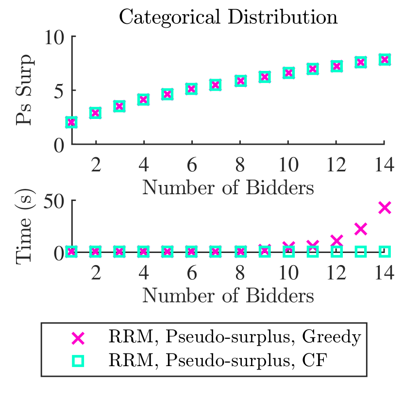
Refer to caption
(a) Categorical Distribution
Refer to caption
(b) Uniform Distribution
Refer to caption
(c) Binomial Distribution
Figure 3: Pseudo-surplus in the Robust Problem

8.2 Pseudo-surplus Scaling in the Robust Problem

We optimize pseudo-surplus in the robust problem, ensuring ex-post feasibility (see Section C.1.2), to see how it scales with the number of bidders. We report the results of the following:

  • (MATLAB) Total expected pseudo-surplus using Algorithm 8 (the closed form), but without calculating payments.

While the closed-form method is nearly instantaneous when the number of bidders is small, it cannot escape the fact that there are exponentially-many allocation variables. (The behavior of the closed-form solution for the heuristic lower bound—see Section 8.3—is identical as we scale the number of bidders.)
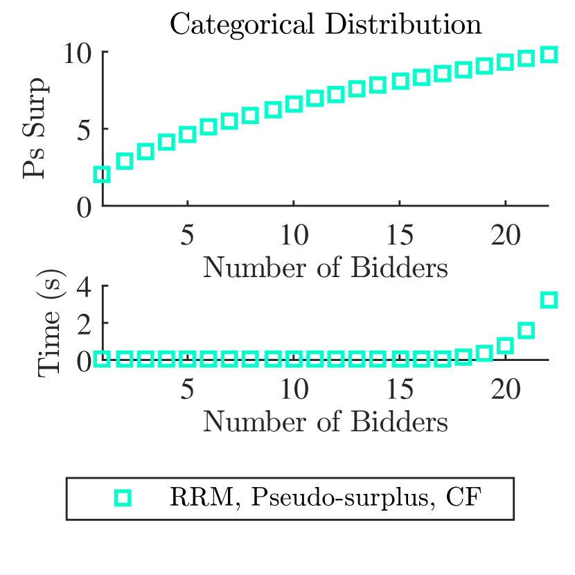
Refer to caption
(a) Categorical Distribution
Refer to caption
(b) Uniform Distribution
Refer to caption
(c) Binomial Distribution
Figure 4: Pseudo-surplus Scaling in the Robust Problem

8.3 Heuristic Lower Bound in the Robust Problem

We optimize the heuristic lower bound ensuring ex-post feasibility (see Section C.1.3). We report the results of the following two methods:

  • (MATLAB) The heuristic lower bound using Algorithm 6 (the greedy method), but without calculating payments.

  • (MATLAB) The heuristic lower bound using Algorithm 9 (the closed form), but without calculating payments.

Both methods achieve the optimal objective value, but using Algorithm 9 (the closed form), we achieve this value more quickly than when using Algorithm 6 (the greedy method).
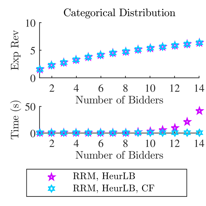
Refer to caption
(a) Categorical Distribution
Refer to caption
(b) Uniform Distribution
Refer to caption
(c) Binomial Distribution
Figure 5: Heuristic Lower Bound in the Robust Problem

8.4 Heuristic Revenue in the Robust Problem

We first optimize our heuristic lower bound in the robust problem (see Section C.1.3). Next, we plug the resulting allocation rule 𝐱𝐱\mathbf{x} into into Myerson’s formula to compute robust payment rule 𝐩𝐩\mathbf{p} (Equation (10)), and then total expected heuristic revenue. Varying the optimization technique, we report the results of the following two methods:

  • (MATLAB) Total expected heuristic revenue using Algorithm 6 (the greedy method) and robust payments (Equation (10)).

  • (MATLAB) Total expected heuristic revenue using Algorithm 9 (the closed form) and robust payments (Equation (10)).

Our choice of discretization factor in our greedy implementation is sufficiently fine that both methods achieve the same objective value. Moreover, the run times of the two methods are not noticeably different, because both are dominated by the exponential number of robust payment calculations. Both these runs are noticeably slower than the pseudo-surplus and heuristic lower bound runs, which perform no payment calculations at all.
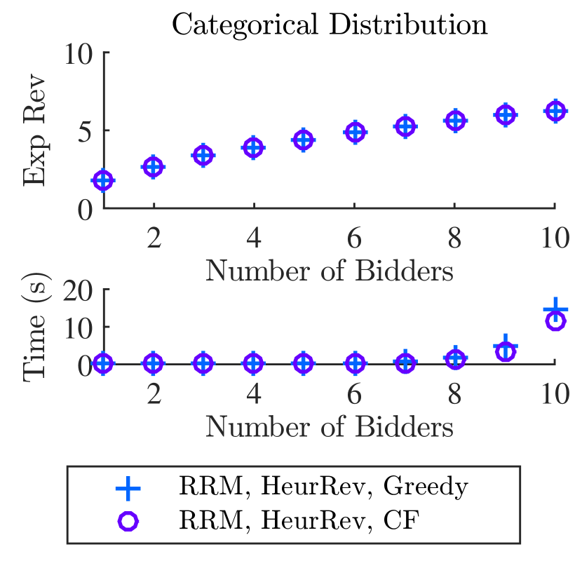
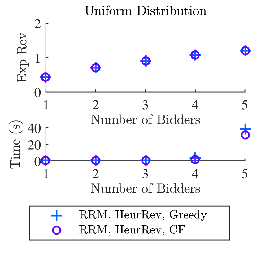
Refer to caption
(a) Categorical Distribution
Refer to caption
(b) Uniform Distribution
Refer to caption
(c) Binomial Distribution
Figure 6: Heuristic Revenue in the Robust Problem

8.5 Heuristic Revenue in the Bayesian Problem

We first optimize our heuristic lower bound in the robust problem (see Section C.1.3). Next we collapse the resulting allocation rule 𝐱𝐱\mathbf{x} into an interim allocation rule 𝐱^^𝐱\hat{\mathbf{x}}. Finally, we plug 𝐱^^𝐱\hat{\mathbf{x}} into Myerson’s formula to compute Bayesian payment rule 𝐡𝐡\mathbf{h} (Equation (11)), and then total expected heuristic revenue. Varying the optimization technique, we report the results of the following two methods:

  • (MATLAB) Total expected heuristic revenue using Algorithm 7 (the greedy method) and Bayesian payments (Equation (11)).

  • (MATLAB) Total expected heuristic revenue using Algorithm 10 (the closed form) and Bayesian payments (Equation (11)).

As above, our choice of discretization factor in our greedy implementation is sufficiently fine that both methods achieve the same objective value. But this time, using Algorithm 10 (the closed form), we achieve this value much more quickly. This is because there are only polynomially-many payment calculations in the Bayesian problem, so the speed up achieved by the closed-form method is not eviscerated by expensive payment calculations.
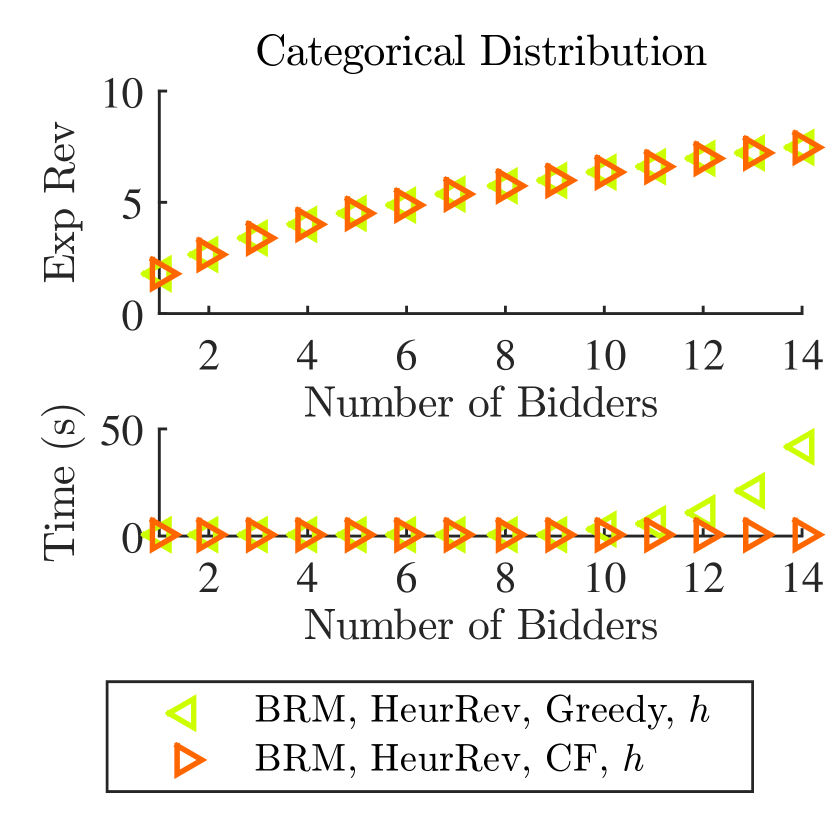
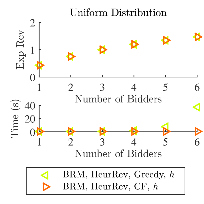
Refer to caption
(a) Categorical Distribution
Refer to caption
(b) Uniform Distribution
Refer to caption
(c) Binomial Distribution
Figure 7: Heuristic Revenue in the Bayesian Problem

8.6 Heuristic Lower Bound and Heuristic Revenue: Robust vs. Bayesian

We compare the heuristic lower bound in the robust problem; total expected heuristic revenue in the robust problem; and total expected heuristic revenue in the Bayesian problem. We report the results of the following three methods:

  • (MATLAB) The heuristic lower bound in the robust problem (see Section C.1.3) using Algorithm 9 (the closed form), but without calculating payments.

  • (MATLAB) Total expected heuristic revenue in the robust problem using Algorithm 9 (the closed form and robust payments using Equation (10)).

  • (MATLAB) Total expected heuristic revenue in the Bayesian problem using Algorithm 10 (the closed form and Bayesian payments using Equation (11)).

According to the theory developed in this paper, the heuristic lower bound in the robust problem should not exceed the heuristic revenue in the robust problem, which in turn should not exceed the heuristic revenue in the Bayesian problem. Our experiments are consistent with these claims, and further provide examples where the heuristic revenue in the robust problem strictly exceeds the heuristic lower bound, and where the heuristic revenue in the Bayesian problem strictly exceeds that of the robust problem.

Moreover, the Bayesian heuristic runs significantly faster than the robust heuristic; this difference can be attributed to the computation of polynomially- instead of exponentially-many payments. (The heuristic lower bound computes no payments at all.)

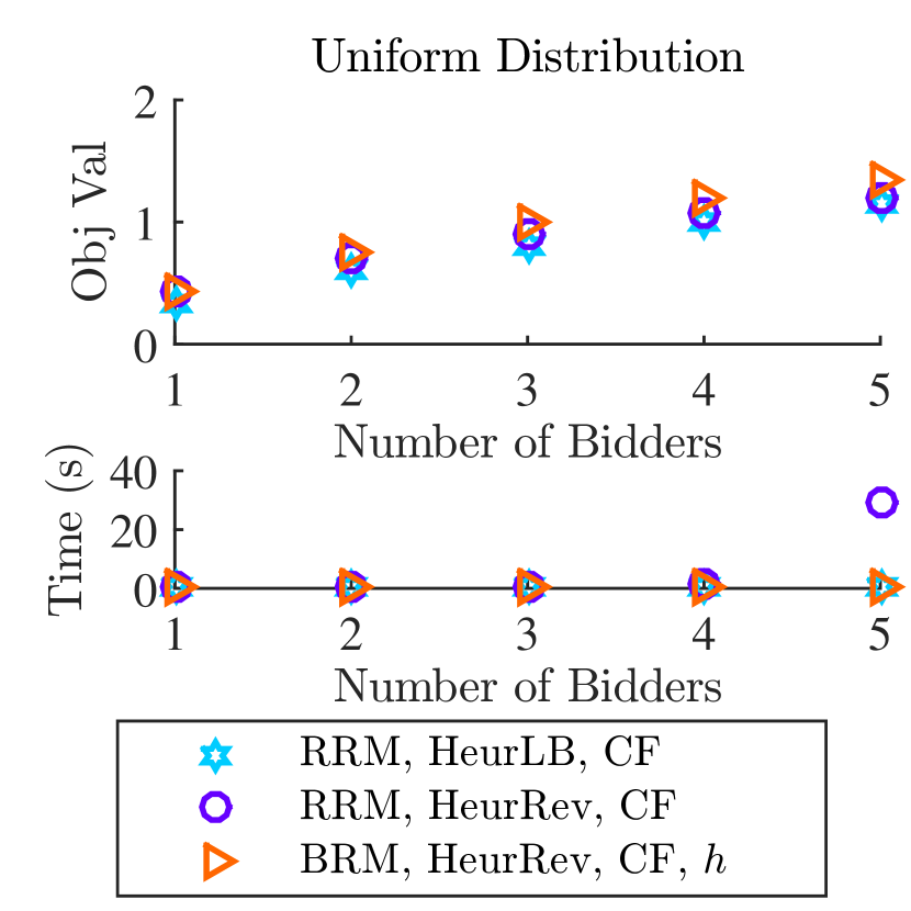
Refer to caption
(a) Categorical Distribution
Refer to caption
(b) Uniform Distribution
Refer to caption
(c) Binomial Distribution
Figure 8: Robust vs. Bayesian Heuristic Revenue

8.7 Revenue, Pseudo-Surplus, and Heuristic Revenue in the Robust Problem

We report the results of the following:

  • (CPLEX) Total expected revenue in the robust problem (see Section C.1.1).

  • (MATLAB) Total expected pseudo-surplus in the robust problem (see Section C.1.2) solved in closed form using Algorithm 8, but without calculating payments.

  • (MATLAB) Total expected heuristic revenue in the robust problem (see Section C.1.3) solved in closed form, and then plugged in to Myerson’s formula for robust payments (Algorithm 9).

CPLEX solves the robust problem optimally, while the other two programs do not. Furthermore, when there are very few bidders (e.g., 1 or 2), CPLEX solves RRM just as fast as MATLAB solves for pseudo-surplus or the heuristic revenue. But as the number of bidders grows, CPLEX does not scale. The heuristic revenue appears to approximate the value of RRM as determined by CPLEX quite well, and it scales better than CPLEX.
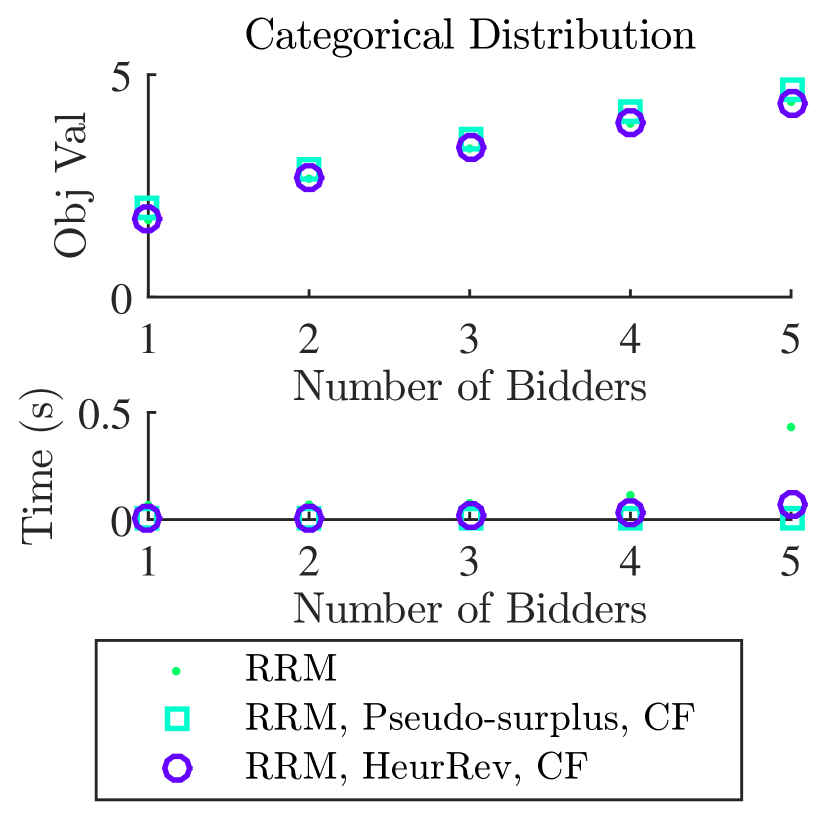
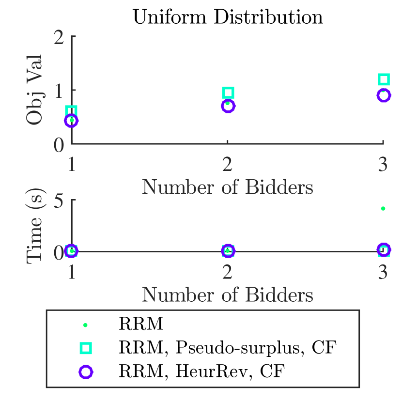
Refer to caption
(a) Categorical Distribution
Refer to caption
(b) Uniform Distribution
Refer to caption
(c) Binomial Distribution
Figure 9: RRM, Pseudo-Surplus, and Heuristic Revenue

8.8 Revenue, Pseudo-Surplus, and Heuristic Revenue in the Bayesian problem

We report the results of the following:

  • (CPLEX) Total expected revenue in the Bayesian problem using Equation (11) (see Section C.2.2).

  • (CPLEX) Total expected pseudo-surplus in the Bayesian problem (see Section C.2.3).

  • (MATLAB) Total expected heuristic revenue in the Bayesian problem (see Section C.2.3, Remark C.1), solved in closed form, and then plugged in to Myerson’s formula for Bayesian payments (Algorithm 10).

CPLEX solves the Bayesian problem optimally, while the other two programs do not. Furthermore, when there are very few bidders (e.g., 1, 2, or 3), CPLEX solves BRM just as fast as CPLEX solves for pseudo-surplus or MATLAB solves for the heuristic revenue. But as the number of bidders grows, CPLEX does not scale. The heuristic revenue appears to approximate the value of BRM as determined by CPLEX quite well, and it scales better than CPLEX.
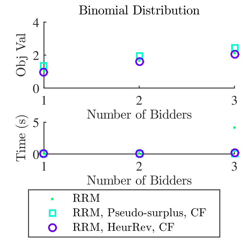
Refer to caption
(a) Categorical Distribution
Refer to caption
(b) Uniform Distribution
Refer to caption
(c) Binomial Distribution
Figure 10: BRM, Pseudo-Surplus, and Heuristic Revenue

8.9 BRM Ex-Ante

We report the results of the following:

  • (CPLEX) Total expected revenue of the BRM ex-ante relaxation (see Section C.3.1).

  • (MATLAB) Total expected revenue of the BRM ex-ante relaxation (see Section C.3.2) solved in closed form (see Theorem 7.1) to find an interim allocation rule, and use it to compute Bayesian payments.

  • (MATLAB) Total expected revenue of the BRM, ex-ante relaxation (see Section C.3.2), solved in closed form (see Theorem 7.1) to find an interim allocation rule, which is then truncated so that x^i(vi)1subscript^𝑥𝑖subscript𝑣𝑖1\hat{x}_{i}(v_{i})\leq 1 for each iN𝑖𝑁i\in N and viTisubscript𝑣𝑖subscript𝑇𝑖v_{i}\in T_{i}, before using it to compute Bayesian payments.

For the BRM ex-ante relaxation, a problem with only polynomially-many variables and constraints, even CPLEX, which is optimal, appears to scale just fine with the number of bidders. Indeed, while the approximations are faster than CPLEX on small problems, their run time eventually grows, while CPLEX does not.
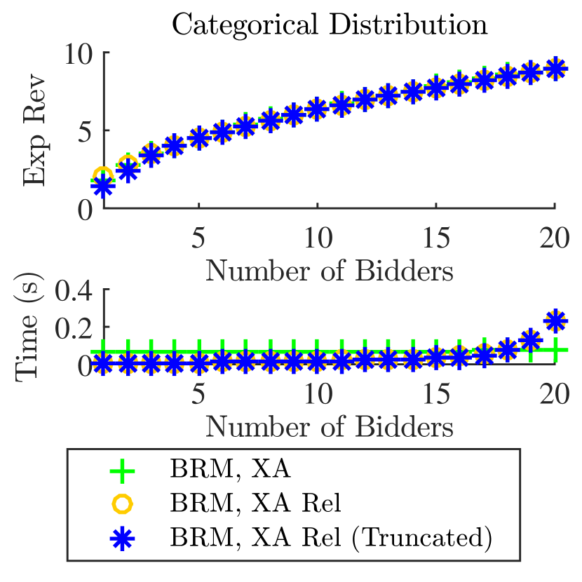
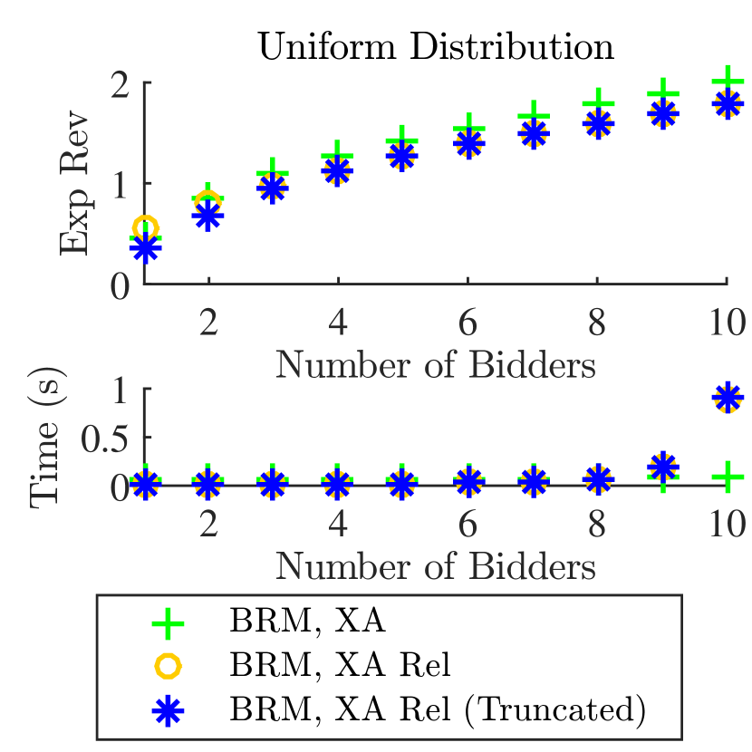
Refer to caption
(a) Categorical Distribution
Refer to caption
(b) Uniform Distribution
Refer to caption
(c) Binomial Distribution
Figure 11: BRM Ex-Ante Variants

9 Conclusion and Future Work

We analyzed optimal auctions where bidder utilities are quasi-linear, but defined in terms of convex, instead of the usual linear, payments. We adapted Myerson’s analysis to this setting when it is required that constraints always hold (i.e., the robust problem) and when it is required only that they hold in expectation (i.e., the Bayesian problem). We showed that total expected revenue in the Bayesian problem can exceed the total expected revenue in the robust problem, and consequently, we analyzed each problem in turn.

In the robust setting, we developed upper and lower bounds on total expected revenue that can be computed easily using the equi-marginal principle. In the Bayesian setting, we derived a payment formula that lends itself to a mathematical program that involves fewer variables than a straightforward implementation of the optimal auction problem. Additionally, we derived closed-form solutions to a relaxation of the Bayesian ex-ante problem, as well as problems that seek robust upper and lower bounds.

Based on our analysis, we derived heuristics that approximate solutions to both the robust and Bayesian revenue maximization problems. With three different distributions, we saw through experiments that our heuristics produce solutions that are close to optimal, and scale better than the mathematical programming solver we used. However, our experiments thus far were restricted to quasi-linear utility functions with quadratic perceived payments. In the future, we hope to run experiments with a wider class of payment functions, beyond quadratic, and possibly even develop theory that goes beyond convex entirely. Additionally, we hope to prove guarantees about our heuristics, to further characterize their quality.

10 Acknowledgments

This research was supported by NSF Grant #1217761 and Microsoft Research. Amy and Takehiro would also like to thank Jason Hartline and Tim Roughgarden for always being willing to help as we grappled with the details of Myerson’s seminal work.

Appendix A The Discretization Effect

Let 𝐱superscript𝐱\mathbf{x}^{*} be an optimal allocation rule in an arbitrary auction design problem, and let 𝐱𝐱\mathbf{x} be an optimal allocation rule in the corresponding discretized problem, with discretization factor Δ>0Δ0\Delta>0. For all bidders iN𝑖𝑁i\in N, let 0ki0subscript𝑘𝑖0\leq k_{i}\in\mathbb{Z} be such that

xi(vi,𝐯i)=kiΔ.subscript𝑥𝑖subscript𝑣𝑖subscript𝐯𝑖subscript𝑘𝑖Δx_{i}(v_{i},\mathbf{v}_{-i})=k_{i}\Delta. (97)

The optimal values xi(vi,𝐯i)superscriptsubscript𝑥𝑖subscript𝑣𝑖subscript𝐯𝑖x_{i}^{*}(v_{i},\mathbf{v}_{-i}) and our approximation xi(vi,𝐯i)subscript𝑥𝑖subscript𝑣𝑖subscript𝐯𝑖x_{i}(v_{i},\mathbf{v}_{-i}) are related by a residual vector 𝝆𝝆\bm{\rho}, each entry of which can be be positive, negative, or zero:

xi(vi,𝐯i)superscriptsubscript𝑥𝑖subscript𝑣𝑖subscript𝐯𝑖\displaystyle x_{i}^{*}(v_{i},\mathbf{v}_{-i}) =xi(vi,𝐯i)+ρiabsentsubscript𝑥𝑖subscript𝑣𝑖subscript𝐯𝑖subscript𝜌𝑖\displaystyle=x_{i}(v_{i},\mathbf{v}_{-i})+\rho_{i} (98)
=kiΔ+ρi,absentsubscript𝑘𝑖Δsubscript𝜌𝑖\displaystyle=k_{i}\Delta+\rho_{i}, (99)

To determine kisubscript𝑘𝑖k_{i}s, we use the method of least squares. Specifically, we minimize the square of the residual L2superscript𝐿2L^{2}-norm:

𝝆22=i=1n(xi(vi,𝐯i)kiΔ)2.superscriptsubscriptdelimited-∥∥𝝆22superscriptsubscript𝑖1𝑛superscriptsuperscriptsubscript𝑥𝑖subscript𝑣𝑖subscript𝐯𝑖subscript𝑘𝑖Δ2\lVert\bm{\rho}\rVert_{2}^{2}=\sum_{i=1}^{n}\left(x_{i}^{*}(v_{i},\mathbf{v}_{-i})-k_{i}\Delta\right)^{2}. (100)

To do so, we take derivatives with respect to kisubscript𝑘𝑖k_{i}:

i=1n(xi(vi,𝐯i)kiΔ)2ki=2(xi(vi,𝐯i)kiΔ)(Δ).superscriptsubscript𝑖1𝑛superscriptsuperscriptsubscript𝑥𝑖subscript𝑣𝑖subscript𝐯𝑖subscript𝑘𝑖Δ2subscript𝑘𝑖2superscriptsubscript𝑥𝑖subscript𝑣𝑖subscript𝐯𝑖subscript𝑘𝑖ΔΔ\frac{\partial\sum_{i=1}^{n}\left(x_{i}^{*}(v_{i},\mathbf{v}_{-i})-k_{i}\Delta\right)^{2}}{\partial k_{i}}=2\left(x_{i}^{*}(v_{i},\mathbf{v}_{-i})-k_{i}\Delta\right)(-\Delta). (101)

Setting the right-hand side of this equation to 0 yields the following intuitive result:

ki=xi(vi,𝐯i)Δ.subscript𝑘𝑖superscriptsubscript𝑥𝑖subscript𝑣𝑖subscript𝐯𝑖Δk_{i}=\frac{x_{i}^{*}(v_{i},\mathbf{v}_{-i})}{\Delta}. (102)

Enforcing the constraint that kisubscript𝑘𝑖k_{i} must be integral leaves two possible candidate kisubscript𝑘𝑖k_{i}s:

ki=xi(vi,𝐯i)Δorki=xi(vi,𝐯i)Δ.formulae-sequencesubscript𝑘𝑖superscriptsubscript𝑥𝑖subscript𝑣𝑖subscript𝐯𝑖Δorsubscript𝑘𝑖superscriptsubscript𝑥𝑖subscript𝑣𝑖subscript𝐯𝑖Δ\displaystyle k_{i}=\left\lfloor{\frac{x_{i}^{*}(v_{i},\mathbf{v}_{-i})}{\Delta}}\right\rfloor\quad\text{or}\quad k_{i}=\left\lceil{\frac{x_{i}^{*}(v_{i},\mathbf{v}_{-i})}{\Delta}}\right\rceil. (103)

In either case,

ρi=xi(vi,𝐯i)xi(vi,𝐯i)|xi(vi,𝐯i)xi(vi,𝐯i)|Δ.subscript𝜌𝑖superscriptsubscript𝑥𝑖subscript𝑣𝑖subscript𝐯𝑖subscript𝑥𝑖subscript𝑣𝑖subscript𝐯𝑖superscriptsubscript𝑥𝑖subscript𝑣𝑖subscript𝐯𝑖subscript𝑥𝑖subscript𝑣𝑖subscript𝐯𝑖Δ\rho_{i}=x_{i}^{*}(v_{i},\mathbf{v}_{-i})-x_{i}(v_{i},\mathbf{v}_{-i})\leq\lvert x_{i}^{*}(v_{i},\mathbf{v}_{-i})-x_{i}(v_{i},\mathbf{v}_{-i})\rvert\leq\Delta. (104)

Therefore, the residual from bidder i𝑖i is bounded above by O(Δ)𝑂ΔO(\Delta). Likewise, the total residual is bounded above by O(nΔ)𝑂𝑛ΔO(n\Delta).

Having established a method of determining 𝐱𝐱\mathbf{x}, we now describe how using 𝐱𝐱\mathbf{x} can impact the total expected perceived payment. Let 𝐪superscript𝐪\mathbf{q}^{*} and 𝐪𝐪\mathbf{q} be the perceived payments resulting from the allocation rules 𝐱superscript𝐱\mathbf{x}^{*} and 𝐱𝐱\mathbf{x}, respectively. First, we show that the difference in expected the perceived payment from bidder i𝑖i when using 𝐱𝐱\mathbf{x} instead of 𝐱superscript𝐱\mathbf{x}^{*} is O(Δ)𝑂ΔO(\Delta). Then, we conclude that the total expected perceived payment is O(nΔ)𝑂𝑛ΔO(n\Delta).

Lemma A.1.

The difference in bidder i𝑖i’s expected perceived payment when using 𝐱𝐱\mathbf{x} instead of 𝐱superscript𝐱\mathbf{x}^{*} is O(Δ)𝑂ΔO(\Delta): i.e., |𝔼zi,Fi[qi(zi,,𝐯i)]𝔼zi,Fi[qi(zi,,𝐯i)]|O(Δ)subscript𝔼similar-tosubscript𝑧𝑖subscript𝐹𝑖superscriptsubscript𝑞𝑖subscript𝑧𝑖subscript𝐯𝑖subscript𝔼similar-tosubscript𝑧𝑖subscript𝐹𝑖subscript𝑞𝑖subscript𝑧𝑖subscript𝐯𝑖𝑂Δ\lvert\operatorname*{\mathbb{E}}_{z_{i,\ell}\sim F_{i}}\left[q_{i}^{*}(z_{i,\ell},\mathbf{v}_{-i})\right]-\operatorname*{\mathbb{E}}_{z_{i,\ell}\sim F_{i}}\left[q_{i}(z_{i,\ell},\mathbf{v}_{-i})\right]\rvert\in O(\Delta).

Proof.

We can express the difference between 𝔼zi,Fi[qi(zi,,𝐯i)]subscript𝔼similar-tosubscript𝑧𝑖subscript𝐹𝑖superscriptsubscript𝑞𝑖subscript𝑧𝑖subscript𝐯𝑖\operatorname*{\mathbb{E}}_{z_{i,\ell}\sim F_{i}}\left[q_{i}^{*}(z_{i,\ell},\mathbf{v}_{-i})\right] and 𝔼zi,Fi[qi(zi,,𝐯i)]subscript𝔼similar-tosubscript𝑧𝑖subscript𝐹𝑖subscript𝑞𝑖subscript𝑧𝑖subscript𝐯𝑖\operatorname*{\mathbb{E}}_{z_{i,\ell}\sim F_{i}}\left[q_{i}(z_{i,\ell},\mathbf{v}_{-i})\right] in terms of virtual values:

𝔼zi,Fi[qi(zi,,𝐯i)]𝔼zi,Fi[qi(zi,,𝐯i)]subscript𝔼similar-tosubscript𝑧𝑖subscript𝐹𝑖superscriptsubscript𝑞𝑖subscript𝑧𝑖subscript𝐯𝑖subscript𝔼similar-tosubscript𝑧𝑖subscript𝐹𝑖subscript𝑞𝑖subscript𝑧𝑖subscript𝐯𝑖\displaystyle\operatorname*{\mathbb{E}}_{z_{i,\ell}\sim F_{i}}\left[q_{i}^{*}(z_{i,\ell},\mathbf{v}_{-i})\right]-\operatorname*{\mathbb{E}}_{z_{i,\ell}\sim F_{i}}\left[q_{i}(z_{i,\ell},\mathbf{v}_{-i})\right] =𝔼zi,Fi[ψi(zi,)xi(zi,,𝐯i)ψi(zi,)xi(zi,,𝐯i)]absentsubscript𝔼similar-tosubscript𝑧𝑖subscript𝐹𝑖subscript𝜓𝑖subscript𝑧𝑖superscriptsubscript𝑥𝑖subscript𝑧𝑖subscript𝐯𝑖subscript𝜓𝑖subscript𝑧𝑖subscript𝑥𝑖subscript𝑧𝑖subscript𝐯𝑖\displaystyle=\operatorname*{\mathbb{E}}_{z_{i,\ell}\sim F_{i}}\left[\psi_{i}(z_{i,\ell})\,x_{i}^{*}(z_{i,\ell},\mathbf{v}_{-i})-\psi_{i}(z_{i,\ell})\,x_{i}(z_{i,\ell},\mathbf{v}_{-i})\right] (105)
=𝔼zi,Fi[ψi(zi,)(xi(zi,,𝐯i)xi(zi,,𝐯i))]absentsubscript𝔼similar-tosubscript𝑧𝑖subscript𝐹𝑖subscript𝜓𝑖subscript𝑧𝑖superscriptsubscript𝑥𝑖subscript𝑧𝑖subscript𝐯𝑖subscript𝑥𝑖subscript𝑧𝑖subscript𝐯𝑖\displaystyle=\operatorname*{\mathbb{E}}_{z_{i,\ell}\sim F_{i}}\left[\psi_{i}(z_{i,\ell})\,\left(x_{i}^{*}(z_{i,\ell},\mathbf{v}_{-i})-x_{i}(z_{i,\ell},\mathbf{v}_{-i})\right)\right] (106)
𝔼zi,Fi[ψi(zi,)Δ]absentsubscript𝔼similar-tosubscript𝑧𝑖subscript𝐹𝑖subscript𝜓𝑖subscript𝑧𝑖Δ\displaystyle\leq\operatorname*{\mathbb{E}}_{z_{i,\ell}\sim F_{i}}\left[\psi_{i}(z_{i,\ell})\,\Delta\right] (107)
O(Δ).absent𝑂Δ\displaystyle\in O(\Delta). (108)

Corollary A.2.

The difference in total expected perceived payment when using 𝐱𝐱\mathbf{x} instead of 𝐱superscript𝐱\mathbf{x}^{*} is O(nΔ)𝑂𝑛ΔO(n\Delta): i.e., |i=1n𝔼𝐯[qi(zi,,𝐯i)qi(zi,,𝐯i)]|O(nΔ)superscriptsubscript𝑖1𝑛subscript𝔼𝐯superscriptsubscript𝑞𝑖subscript𝑧𝑖subscript𝐯𝑖subscript𝑞𝑖subscript𝑧𝑖subscript𝐯𝑖𝑂𝑛Δ\lvert\sum_{i=1}^{n}\operatorname*{\mathbb{E}}_{\mathbf{v}}\left[q_{i}^{*}(z_{i,\ell},\mathbf{v}_{-i})-q_{i}(z_{i,\ell},\mathbf{v}_{-i})\right]\rvert\in O(n\Delta).

En route to deriving the difference in total expected revenue from using allocation rule 𝐱𝐱\mathbf{x} instead of 𝐱superscript𝐱\mathbf{x}^{*}, we present the following lemma, which argues that the maximum difference in perceived payment from bidder i𝑖i is O(Δ)𝑂ΔO(\Delta).

Lemma A.3.

The difference in bidder i𝑖i’s perceived payment when using allocation rule 𝐱𝐱\mathbf{x} instead of 𝐱superscript𝐱\mathbf{x}^{*} is O(Δ)𝑂ΔO(\Delta): i.e., |qi(zi,,𝐯i)qi(zi,,𝐯i)|O(Δ)superscriptsubscript𝑞𝑖subscript𝑧𝑖subscript𝐯𝑖subscript𝑞𝑖subscript𝑧𝑖subscript𝐯𝑖𝑂Δ\lvert q_{i}^{*}(z_{i,\ell},\mathbf{v}_{-i})-q_{i}(z_{i,\ell},\mathbf{v}_{-i})\rvert\in O(\Delta).

Proof.

Without loss of generality, assume qi(zi,,𝐯i)qi(zi,,𝐯i)superscriptsubscript𝑞𝑖subscript𝑧𝑖subscript𝐯𝑖subscript𝑞𝑖subscript𝑧𝑖subscript𝐯𝑖q_{i}^{*}(z_{i,\ell},\mathbf{v}_{-i})\geq q_{i}(z_{i,\ell},\mathbf{v}_{-i}). Allocation variables xi(zi,,𝐯i)superscriptsubscript𝑥𝑖subscript𝑧𝑖subscript𝐯𝑖x_{i}^{*}(z_{i,\ell},\mathbf{v}_{-i}) and xi(zi,,𝐯i)subscript𝑥𝑖subscript𝑧𝑖subscript𝐯𝑖x_{i}(z_{i,\ell},\mathbf{v}_{-i}) can differ by at most ΔΔ\Delta, so the difference between qi(zi,,𝐯i)superscriptsubscript𝑞𝑖subscript𝑧𝑖subscript𝐯𝑖q_{i}^{*}(z_{i,\ell},\mathbf{v}_{-i}) and qi(zi,,𝐯i)subscript𝑞𝑖subscript𝑧𝑖subscript𝐯𝑖q_{i}(z_{i,\ell},\mathbf{v}_{-i}) is maximized when xi(zi,,𝐯i)=xi(zi,,𝐯i)+Δsuperscriptsubscript𝑥𝑖subscript𝑧𝑖subscript𝐯𝑖subscript𝑥𝑖subscript𝑧𝑖subscript𝐯𝑖Δx_{i}^{*}(z_{i,\ell},\mathbf{v}_{-i})=x_{i}(z_{i,\ell},\mathbf{v}_{-i})+\Delta, for an arbitrary value \ell, and xi(zi,j,𝐯i)=xi(zi,j,𝐯i)Δsuperscriptsubscript𝑥𝑖subscript𝑧𝑖𝑗subscript𝐯𝑖subscript𝑥𝑖subscript𝑧𝑖𝑗subscript𝐯𝑖Δx_{i}^{*}(z_{i,j},\mathbf{v}_{-i})=x_{i}(z_{i,j},\mathbf{v}_{-i})-\Delta, for j<𝑗j<\ell. Now

qi(zi,,𝐯i)superscriptsubscript𝑞𝑖subscript𝑧𝑖subscript𝐯𝑖\displaystyle q_{i}^{*}(z_{i,\ell},\mathbf{v}_{-i}) =(zi,xi(zi,,𝐯i)j=11(zi,j+1zi,j)xi(zi,j,𝐯i))absentsubscript𝑧𝑖superscriptsubscript𝑥𝑖subscript𝑧𝑖subscript𝐯𝑖superscriptsubscript𝑗11subscript𝑧𝑖𝑗1subscript𝑧𝑖𝑗superscriptsubscript𝑥𝑖subscript𝑧𝑖𝑗subscript𝐯𝑖\displaystyle=\left(z_{i,\ell}x_{i}^{*}(z_{i,\ell},\mathbf{v}_{-i})-\sum_{j=1}^{\ell-1}(z_{i,j+1}-z_{i,j})x_{i}^{*}(z_{i,j},\mathbf{v}_{-i})\right) (109)
=(zi,(xi(zi,,𝐯i)+Δ)j=11(zi,j+1zi,j)(xi(zi,j,𝐯i)Δ))absentsubscript𝑧𝑖subscript𝑥𝑖subscript𝑧𝑖subscript𝐯𝑖Δsuperscriptsubscript𝑗11subscript𝑧𝑖𝑗1subscript𝑧𝑖𝑗subscript𝑥𝑖subscript𝑧𝑖𝑗subscript𝐯𝑖Δ\displaystyle=\left(z_{i,\ell}(x_{i}(z_{i,\ell},\mathbf{v}_{-i})+\Delta)-\sum_{j=1}^{\ell-1}(z_{i,j+1}-z_{i,j})(x_{i}(z_{i,j},\mathbf{v}_{-i})-\Delta)\right) (110)
=zi,(xi(zi,,𝐯i)j=11(zi,j+1zi,j)xi(zi,j,𝐯i)+zi,Δ+j=11(zi,j+1zi,j)Δ\displaystyle=z_{i,\ell}(x_{i}(z_{i,\ell},\mathbf{v}_{-i})-\sum_{j=1}^{\ell-1}(z_{i,j+1}-z_{i,j})x_{i}(z_{i,j},\mathbf{v}_{-i})+z_{i,\ell}\Delta+\sum_{j=1}^{\ell-1}(z_{i,j+1}-z_{i,j})\Delta (111)
=qi(zi,,𝐯i)+zi,Δ+j=11(zi,j+1zi,j)Δabsentsubscript𝑞𝑖subscript𝑧𝑖subscript𝐯𝑖subscript𝑧𝑖Δsuperscriptsubscript𝑗11subscript𝑧𝑖𝑗1subscript𝑧𝑖𝑗Δ\displaystyle=q_{i}(z_{i,\ell},\mathbf{v}_{-i})+z_{i,\ell}\Delta+\sum_{j=1}^{\ell-1}(z_{i,j+1}-z_{i,j})\Delta (112)
=qi(zi,,𝐯i)+zi,Δ+(zi,zi,1)Δabsentsubscript𝑞𝑖subscript𝑧𝑖subscript𝐯𝑖subscript𝑧𝑖Δsubscript𝑧𝑖subscript𝑧𝑖1Δ\displaystyle=q_{i}(z_{i,\ell},\mathbf{v}_{-i})+z_{i,\ell}\Delta+\left(z_{i,\ell}-z_{i,1}\right)\Delta (113)
=qi(zi,,𝐯i)+Δ(2zi,zi,1)absentsubscript𝑞𝑖subscript𝑧𝑖subscript𝐯𝑖Δ2subscript𝑧𝑖subscript𝑧𝑖1\displaystyle=q_{i}(z_{i,\ell},\mathbf{v}_{-i})+\Delta\left(2z_{i,\ell}-z_{i,1}\right) (114)
=qi(zi,,𝐯i)+O(Δ).absentsubscript𝑞𝑖subscript𝑧𝑖subscript𝐯𝑖𝑂Δ\displaystyle=q_{i}(z_{i,\ell},\mathbf{v}_{-i})+O(\Delta). (115)

Therefore, the difference in perceived payments is O(Δ)𝑂ΔO(\Delta). ∎

Having established Lemma A.3, we now show that discretization affects the expected revenue collected from bidder i𝑖i by O(Δ)𝑂ΔO\left(\sqrt{\Delta}\right), and total expected revenue by O(nΔ)𝑂𝑛ΔO\left(n\sqrt{\Delta}\right).

Lemma A.4.

The difference in expected revenue from bidder i𝑖i when using 𝐱𝐱\mathbf{x} instead of 𝐱superscript𝐱\mathbf{x}^{*} is O(Δ)𝑂ΔO(\sqrt{\Delta}): i.e., |𝔼zi,Fi[pi(zi,,𝐯i)pi(zi,,𝐯i)]|O(Δ).subscript𝔼similar-tosubscript𝑧𝑖subscript𝐹𝑖superscriptsubscript𝑝𝑖subscript𝑧𝑖subscript𝐯𝑖subscript𝑝𝑖subscript𝑧𝑖subscript𝐯𝑖𝑂Δ\lvert\operatorname*{\mathbb{E}}_{z_{i,\ell}\sim F_{i}}\left[p_{i}^{*}(z_{i,\ell},\mathbf{v}_{-i})-p_{i}(z_{i,\ell},\mathbf{v}_{-i})\right]\rvert\in O\left(\sqrt{\Delta}\right).

Proof.

First, we construct payment rules 𝐩¯n¯𝐩superscript𝑛\bar{\mathbf{p}}\in\mathbb{R}^{n} and 𝐩~n~𝐩superscript𝑛\tilde{\mathbf{p}}\in\mathbb{R}^{n}. We choose p¯i(zi,,𝐯i)subscript¯𝑝𝑖subscript𝑧𝑖subscript𝐯𝑖\bar{p}_{i}(z_{i,\ell},\mathbf{v}_{-i}) and p~i(zi,,𝐯i)subscript~𝑝𝑖subscript𝑧𝑖subscript𝐯𝑖\tilde{p}_{i}(z_{i,\ell},\mathbf{v}_{-i}), for all iN𝑖𝑁i\in N and 𝐯T𝐯𝑇\mathbf{v}\in T, so that

p¯i(zi,,𝐯i)subscript¯𝑝𝑖subscript𝑧𝑖subscript𝐯𝑖\displaystyle\bar{p}_{i}(z_{i,\ell},\mathbf{v}_{-i}) =min{pi(zi,,𝐯i),pi(zi,,𝐯i)}absentsuperscriptsubscript𝑝𝑖subscript𝑧𝑖subscript𝐯𝑖subscript𝑝𝑖subscript𝑧𝑖subscript𝐯𝑖\displaystyle=\min\left\{p_{i}^{*}(z_{i,\ell},\mathbf{v}_{-i}),p_{i}(z_{i,\ell},\mathbf{v}_{-i})\right\} (116)
p~i(zi,,𝐯i)subscript~𝑝𝑖subscript𝑧𝑖subscript𝐯𝑖\displaystyle\tilde{p}_{i}(z_{i,\ell},\mathbf{v}_{-i}) =max{pi(zi,,𝐯i),pi(zi,,𝐯i)}.absentsuperscriptsubscript𝑝𝑖subscript𝑧𝑖subscript𝐯𝑖subscript𝑝𝑖subscript𝑧𝑖subscript𝐯𝑖\displaystyle=\max\left\{p_{i}^{*}(z_{i,\ell},\mathbf{v}_{-i}),p_{i}(z_{i,\ell},\mathbf{v}_{-i})\right\}. (117)

Likewise, for 𝐪¯,𝐪~n¯𝐪~𝐪superscript𝑛\bar{\mathbf{q}},\tilde{\mathbf{q}}\in\mathbb{R}^{n}.

By Jensen’s inequality, we can write the difference in expected revenue from bidder i𝑖i as

𝔼zi,Fi[pi(zi,,𝐯i)pi(zi,,𝐯i)]subscript𝔼similar-tosubscript𝑧𝑖subscript𝐹𝑖superscriptsubscript𝑝𝑖subscript𝑧𝑖subscript𝐯𝑖subscript𝑝𝑖subscript𝑧𝑖subscript𝐯𝑖\displaystyle\operatorname*{\mathbb{E}}_{z_{i,\ell}\sim F_{i}}\left[p_{i}^{*}(z_{i,\ell},\mathbf{v}_{-i})-p_{i}(z_{i,\ell},\mathbf{v}_{-i})\right] (118)
(𝔼zi,Fi[(pi(zi,,𝐯i)pi(zi,,𝐯i))2])1/2absentsuperscriptsubscript𝔼similar-tosubscript𝑧𝑖subscript𝐹𝑖superscriptsuperscriptsubscript𝑝𝑖subscript𝑧𝑖subscript𝐯𝑖subscript𝑝𝑖subscript𝑧𝑖subscript𝐯𝑖212\displaystyle\quad\leq\left(\operatorname*{\mathbb{E}}_{z_{i,\ell}\sim F_{i}}\left[\left(p_{i}^{*}(z_{i,\ell},\mathbf{v}_{-i})-p_{i}(z_{i,\ell},\mathbf{v}_{-i})\right)^{2}\right]\right)^{1/2}
=(𝔼zi,Fi[(pi(zi,,𝐯i))22pi(zi,,𝐯i)pi(zi,,𝐯i)+(pi(zi,,𝐯i))2])1/2absentsuperscriptsubscript𝔼similar-tosubscript𝑧𝑖subscript𝐹𝑖superscriptsuperscriptsubscript𝑝𝑖subscript𝑧𝑖subscript𝐯𝑖22superscriptsubscript𝑝𝑖subscript𝑧𝑖subscript𝐯𝑖subscript𝑝𝑖subscript𝑧𝑖subscript𝐯𝑖superscriptsubscript𝑝𝑖subscript𝑧𝑖subscript𝐯𝑖212\displaystyle\quad=\left(\operatorname*{\mathbb{E}}_{z_{i,\ell}\sim F_{i}}\left[\left(p_{i}^{*}(z_{i,\ell},\mathbf{v}_{-i})\right)^{2}-2p_{i}^{*}(z_{i,\ell},\mathbf{v}_{-i})p_{i}(z_{i,\ell},\mathbf{v}_{-i})+\left(p_{i}(z_{i,\ell},\mathbf{v}_{-i})\right)^{2}\right]\right)^{1/2} (119)
(2𝔼zi,Fi[(p~i(zi,,𝐯i))2(p¯i(zi,,𝐯i))2])1/2,absentsuperscript2subscript𝔼similar-tosubscript𝑧𝑖subscript𝐹𝑖superscriptsubscript~𝑝𝑖subscript𝑧𝑖subscript𝐯𝑖2superscriptsubscript¯𝑝𝑖subscript𝑧𝑖subscript𝐯𝑖212\displaystyle\quad\leq\Big{(}2\operatorname*{\mathbb{E}}_{z_{i,\ell}\sim F_{i}}\left[\left(\tilde{p}_{i}(z_{i,\ell},\mathbf{v}_{-i})\right)^{2}-\left(\bar{p}_{i}(z_{i,\ell},\mathbf{v}_{-i})\right)^{2}\right]\Big{)}^{1/2}, (120)

where Equation (120) follows from Equations (116) and (117) and

𝔼zi,Fi[p¯i(zi,,𝐯i)2]subscript𝔼similar-tosubscript𝑧𝑖subscript𝐹𝑖subscript¯𝑝𝑖superscriptsubscript𝑧𝑖subscript𝐯𝑖2\displaystyle\operatorname*{\mathbb{E}}_{z_{i,\ell}\sim F_{i}}\left[\bar{p}_{i}(z_{i,\ell},\mathbf{v}_{-i})^{2}\right] 𝔼zi,Fi[pi(zi,,𝐯i)pi(zi,,𝐯i)]absentsubscript𝔼similar-tosubscript𝑧𝑖subscript𝐹𝑖superscriptsubscript𝑝𝑖subscript𝑧𝑖subscript𝐯𝑖subscript𝑝𝑖subscript𝑧𝑖subscript𝐯𝑖\displaystyle\leq\operatorname*{\mathbb{E}}_{z_{i,\ell}\sim F_{i}}\left[p_{i}^{*}(z_{i,\ell},\mathbf{v}_{-i})p_{i}(z_{i,\ell},\mathbf{v}_{-i})\right] (121)
𝔼zi,Fi[p~i(zi,,𝐯i)2]subscript𝔼similar-tosubscript𝑧𝑖subscript𝐹𝑖subscript~𝑝𝑖superscriptsubscript𝑧𝑖subscript𝐯𝑖2\displaystyle\operatorname*{\mathbb{E}}_{z_{i,\ell}\sim F_{i}}\left[\tilde{p}_{i}(z_{i,\ell},\mathbf{v}_{-i})^{2}\right] 𝔼zi,Fi[(pi(zi,,𝐯i))2]absentsubscript𝔼similar-tosubscript𝑧𝑖subscript𝐹𝑖superscriptsuperscriptsubscript𝑝𝑖subscript𝑧𝑖subscript𝐯𝑖2\displaystyle\geq\operatorname*{\mathbb{E}}_{z_{i,\ell}\sim F_{i}}\left[\left(p_{i}^{*}(z_{i,\ell},\mathbf{v}_{-i})\right)^{2}\right] (122)
𝔼zi,Fi[p~i(zi,,𝐯i)2]subscript𝔼similar-tosubscript𝑧𝑖subscript𝐹𝑖subscript~𝑝𝑖superscriptsubscript𝑧𝑖subscript𝐯𝑖2\displaystyle\operatorname*{\mathbb{E}}_{z_{i,\ell}\sim F_{i}}\left[\tilde{p}_{i}(z_{i,\ell},\mathbf{v}_{-i})^{2}\right] 𝔼zi,Fi[(pi(zi,,𝐯i))2].absentsubscript𝔼similar-tosubscript𝑧𝑖subscript𝐹𝑖superscriptsubscript𝑝𝑖subscript𝑧𝑖subscript𝐯𝑖2\displaystyle\geq\operatorname*{\mathbb{E}}_{z_{i,\ell}\sim F_{i}}\left[\left(p_{i}(z_{i,\ell},\mathbf{v}_{-i})\right)^{2}\right]. (123)

Using Lemma A.3, we arrive at our result:

(2𝔼zi,Fi[(p~i(zi,,𝐯i))2(p¯i(zi,,𝐯i))2])1/2superscript2subscript𝔼similar-tosubscript𝑧𝑖subscript𝐹𝑖superscriptsubscript~𝑝𝑖subscript𝑧𝑖subscript𝐯𝑖2superscriptsubscript¯𝑝𝑖subscript𝑧𝑖subscript𝐯𝑖212\displaystyle\left(2\operatorname*{\mathbb{E}}_{z_{i,\ell}\sim F_{i}}\left[\left(\tilde{p}_{i}(z_{i,\ell},\mathbf{v}_{-i})\right)^{2}-\left(\bar{p}_{i}(z_{i,\ell},\mathbf{v}_{-i})\right)^{2}\right]\right)^{1/2} =(2𝔼zi,Fi[q~i(zi,,𝐯i)q¯i(zi,,𝐯i)])1/2absentsuperscript2subscript𝔼similar-tosubscript𝑧𝑖subscript𝐹𝑖subscript~𝑞𝑖subscript𝑧𝑖subscript𝐯𝑖subscript¯𝑞𝑖subscript𝑧𝑖subscript𝐯𝑖12\displaystyle=\left(2\operatorname*{\mathbb{E}}_{z_{i,\ell}\sim F_{i}}\left[\tilde{q}_{i}(z_{i,\ell},\mathbf{v}_{-i})-\bar{q}_{i}(z_{i,\ell},\mathbf{v}_{-i})\right]\right)^{1/2} (124)
(2𝔼zi,Fi[|qi(zi,,𝐯i)qi(zi,,𝐯i)|])1/2absentsuperscript2subscript𝔼similar-tosubscript𝑧𝑖subscript𝐹𝑖superscriptsubscript𝑞𝑖subscript𝑧𝑖subscript𝐯𝑖subscript𝑞𝑖subscript𝑧𝑖subscript𝐯𝑖12\displaystyle\leq\left(2\operatorname*{\mathbb{E}}_{z_{i,\ell}\sim F_{i}}\left[\lvert q_{i}^{*}(z_{i,\ell},\mathbf{v}_{-i})-q_{i}(z_{i,\ell},\mathbf{v}_{-i})\rvert\right]\right)^{1/2} (125)
(2𝔼zi,Fi[O(Δ)])1/2absentsuperscript2subscript𝔼similar-tosubscript𝑧𝑖subscript𝐹𝑖𝑂Δ12\displaystyle\leq\left(2\ \operatorname*{\mathbb{E}}_{z_{i,\ell}\sim F_{i}}\left[O(\Delta)\right]\right)^{1/2} (126)
O(Δ).absent𝑂Δ\displaystyle\in O\left(\sqrt{\Delta}\right). (127)

Corollary A.5.

The difference in total expected revenue when using 𝐱𝐱\mathbf{x} instead of 𝐱superscript𝐱\mathbf{x}^{*} is O(nΔ)𝑂𝑛ΔO\left(n\sqrt{\Delta}\right): i.e., |i=1n𝔼𝐯[pi(zi,,𝐯i)pi(zi,,𝐯i)]|O(nΔ)superscriptsubscript𝑖1𝑛subscript𝔼𝐯superscriptsubscript𝑝𝑖subscript𝑧𝑖subscript𝐯𝑖subscript𝑝𝑖subscript𝑧𝑖subscript𝐯𝑖𝑂𝑛Δ\lvert\sum_{i=1}^{n}\operatorname*{\mathbb{E}}_{\mathbf{v}}\left[p_{i}^{*}(z_{i,\ell},\mathbf{v}_{-i})-p_{i}(z_{i,\ell},\mathbf{v}_{-i})\right]\rvert\in O\left(n\sqrt{\Delta}\right).

To summarize, in our setting, where a budget B𝐵B is finitely divisible by a factor ΔBsubscriptΔ𝐵\Delta_{B}, so that allocations are multiplicative factors of Δ=ΔB/BΔsubscriptΔ𝐵𝐵\Delta=\Delta_{B}/B, in the usual linear case, where qi=pisubscript𝑞𝑖subscript𝑝𝑖q_{i}=p_{i}, total expected revenue is within O(nΔB/B)𝑂𝑛subscriptΔ𝐵𝐵O\left(n\Delta_{B}/B\right) of optimal. Furthermore, in the case of quadratic perceived payments, total revenue is within O(nΔB/B)𝑂𝑛subscriptΔ𝐵𝐵O\left(n\sqrt{\Delta_{B}/B}\right) of optimal.

Appendix B Another Upper Bound

While non-operational as of yet, we present an easy-to-derive upper bound on revenue for completeness.

Lemma B.1.

Expected payments, when bidders have quasi-linear utility functions as described by Equation (1) and qi(pi(zi,k,𝐯i))=(pi(zi,k,𝐯i))2subscript𝑞𝑖subscript𝑝𝑖subscript𝑧𝑖𝑘subscript𝐯𝑖superscriptsubscript𝑝𝑖subscript𝑧𝑖𝑘subscript𝐯𝑖2q_{i}(p_{i}(z_{i,k},\mathbf{v}_{-i}))=\left(p_{i}(z_{i,k},\mathbf{v}_{-i})\right)^{2}, can be upper-bounded as follows:

𝔼zi,kFi[ψi,kxi(zi,k,𝐯i)]𝔼zi,kFi[pi(zi,k,𝐯i)].subscript𝔼similar-tosubscript𝑧𝑖𝑘subscript𝐹𝑖subscript𝜓𝑖𝑘subscript𝑥𝑖subscript𝑧𝑖𝑘subscript𝐯𝑖subscript𝔼similar-tosubscript𝑧𝑖𝑘subscript𝐹𝑖subscript𝑝𝑖subscript𝑧𝑖𝑘subscript𝐯𝑖\sqrt{\operatorname*{\mathbb{E}}_{z_{i,k}\sim F_{i}}\left[\psi_{i,k}\,x_{i}(z_{i,k},\mathbf{v}_{-i})\right]}\geq\operatorname*{\mathbb{E}}_{z_{i,k}\sim F_{i}}\left[p_{i}(z_{i,k},\mathbf{v}_{-i})\right]. (128)
Proof.

Applying Theorem 5.2 to concave utilities with qi(zi,k,𝐯i)=(pi(zi,k,𝐯i))2subscript𝑞𝑖subscript𝑧𝑖𝑘subscript𝐯𝑖superscriptsubscript𝑝𝑖subscript𝑧𝑖𝑘subscript𝐯𝑖2q_{i}(z_{i,k},\mathbf{v}_{-i})=(p_{i}(z_{i,k},\mathbf{v}_{-i}))^{2} yields:

𝔼zi,kFi[(pi(zi,k,𝐯i))2]=𝔼zi,kFi[ψi,kxi(zi,k,𝐯i)].subscript𝔼similar-tosubscript𝑧𝑖𝑘subscript𝐹𝑖superscriptsubscript𝑝𝑖subscript𝑧𝑖𝑘subscript𝐯𝑖2subscript𝔼similar-tosubscript𝑧𝑖𝑘subscript𝐹𝑖subscript𝜓𝑖𝑘subscript𝑥𝑖subscript𝑧𝑖𝑘subscript𝐯𝑖\operatorname*{\mathbb{E}}_{z_{i,k}\sim F_{i}}\left[(p_{i}(z_{i,k},\mathbf{v}_{-i}))^{2}\right]=\operatorname*{\mathbb{E}}_{z_{i,k}\sim F_{i}}\left[\psi_{i,k}\,x_{i}(z_{i,k},\mathbf{v}_{-i})\right].

By Jensen’s inequality (since squaring is a convex function):

𝔼zi,kFi[(pi(zi,k,𝐯i))2](𝔼zi,kFi[pi(zi,k,𝐯i)])2.subscript𝔼similar-tosubscript𝑧𝑖𝑘subscript𝐹𝑖superscriptsubscript𝑝𝑖subscript𝑧𝑖𝑘subscript𝐯𝑖2superscriptsubscript𝔼similar-tosubscript𝑧𝑖𝑘subscript𝐹𝑖subscript𝑝𝑖subscript𝑧𝑖𝑘subscript𝐯𝑖2\operatorname*{\mathbb{E}}_{z_{i,k}\sim F_{i}}\left[(p_{i}(z_{i,k},\mathbf{v}_{-i}))^{2}\right]\geq\left(\operatorname*{\mathbb{E}}_{z_{i,k}\sim F_{i}}\left[p_{i}(z_{i,k},\mathbf{v}_{-i})\right]\right)^{2}.

Combining the two equations and taking square roots completes the proof. ∎

Example B.2.

Following up on Example 5.5, we again assume Ti={1}subscript𝑇𝑖1T_{i}=\{1\}, for all bidders iN𝑖𝑁i\in N, so that ψi,1=1subscript𝜓𝑖11\psi_{i,1}=1. In this case, the upper bound (Equation (128)) is tight:

ψi,1xi(vi,𝐯i)=(1)(1n)=1n=pi(vi,𝐯i).subscript𝜓𝑖1subscript𝑥𝑖subscript𝑣𝑖subscript𝐯𝑖11𝑛1𝑛subscript𝑝𝑖subscript𝑣𝑖subscript𝐯𝑖\sqrt{\psi_{i,1}\,x_{i}(v_{i},\mathbf{v}_{-i})}=\sqrt{(1)\left(\frac{1}{n}\right)}=\sqrt{\frac{1}{n}}=p_{i}(v_{i},\mathbf{v}_{-i}).

Appendix C Program Descriptions

We describe the programs implemented, including the number of variables and constraints. Let k=maxi{Mi:iN}𝑘subscript𝑖:subscript𝑀𝑖𝑖𝑁k=\max_{i}\{M_{i}:i\in N\}, so that kMi𝑘subscript𝑀𝑖k\geq M_{i}, for all bidders iN𝑖𝑁i\in N.

C.1 RRM Mathematical Programs

C.1.1 RRM

Mathematical Program
max𝐱subscript𝐱\displaystyle\max_{\mathbf{x}}\, 𝐯i=1nf(𝐯)pi(𝐯)subscript𝐯superscriptsubscript𝑖1𝑛𝑓𝐯subscript𝑝𝑖𝐯\displaystyle\sum_{\mathbf{v}}\sum_{i=1}^{n}f(\mathbf{v})p_{i}(\mathbf{v}) (129)
subject to i=1nxi(𝐯)1,superscriptsubscript𝑖1𝑛subscript𝑥𝑖𝐯1\displaystyle\sum_{i=1}^{n}x_{i}(\mathbf{v})\leq 1, 𝐯Tfor-all𝐯𝑇\displaystyle\forall\mathbf{v}\in T (130)
0xi(𝐯),0subscript𝑥𝑖𝐯\displaystyle 0\leq x_{i}(\mathbf{v}), iN,𝐯Tformulae-sequencefor-all𝑖𝑁for-all𝐯𝑇\displaystyle\forall i\in N,\forall\mathbf{v}\in T (131)
xi(𝐯)1,subscript𝑥𝑖𝐯1\displaystyle x_{i}(\mathbf{v})\leq 1, iN,𝐯Tformulae-sequencefor-all𝑖𝑁for-all𝐯𝑇\displaystyle\forall i\in N,\forall\mathbf{v}\in T (132)
xi(zi,,𝐯i)xi(zi,1,𝐯i),subscript𝑥𝑖subscript𝑧𝑖subscript𝐯𝑖subscript𝑥𝑖subscript𝑧𝑖1subscript𝐯𝑖\displaystyle x_{i}(z_{i,\ell},\mathbf{v}_{-i})\geq x_{i}(z_{i,\ell-1},\mathbf{v}_{-i}), iN,zi,>zi,1Ti,𝐯iTiformulae-sequenceformulae-sequencefor-all𝑖𝑁for-allsubscript𝑧𝑖subscript𝑧𝑖1subscript𝑇𝑖for-allsubscript𝐯𝑖subscript𝑇𝑖\displaystyle\forall i\in N,\forall z_{i,\ell}>z_{i,\ell-1}\in T_{i},\forall\mathbf{v}_{-i}\in T_{-i} (133)
(pi(zi,,𝐯i))2=zi,xi(zi,,𝐯i)superscriptsubscript𝑝𝑖subscript𝑧𝑖subscript𝐯𝑖2limit-fromsubscript𝑧𝑖subscript𝑥𝑖subscript𝑧𝑖subscript𝐯𝑖\displaystyle\left(p_{i}(z_{i,\ell},\mathbf{v}_{-i})\right)^{2}=z_{i,\ell}x_{i}(z_{i,\ell},\mathbf{v}_{-i})- (134)
j=11(zi,j+1zi,j)x^i(zi,j,𝐯i),superscriptsubscript𝑗11subscript𝑧𝑖𝑗1subscript𝑧𝑖𝑗subscript^𝑥𝑖subscript𝑧𝑖𝑗subscript𝐯𝑖\displaystyle\qquad\sum_{j=1}^{\ell-1}(z_{i,j+1}-z_{i,j})\hat{x}_{i}(z_{i,j},\mathbf{v}_{-i}), iN,zi,Ti,𝐯iTiformulae-sequencefor-all𝑖𝑁formulae-sequencefor-allsubscript𝑧𝑖subscript𝑇𝑖for-allsubscript𝐯𝑖subscript𝑇𝑖\displaystyle\forall i\in N,\forall z_{i,\ell}\in T_{i},\forall\mathbf{v}_{-i}\in T_{-i}
Variables

For each bidder iN𝑖𝑁i\in N, and for each 𝐯T𝐯𝑇\mathbf{v}\in T, there are variables xi(vi,𝐯i)subscript𝑥𝑖subscript𝑣𝑖subscript𝐯𝑖x_{i}(v_{i},\mathbf{v}_{-i}) and pi(vi,𝐯i)subscript𝑝𝑖subscript𝑣𝑖subscript𝐯𝑖p_{i}(v_{i},\mathbf{v}_{-i}). The total number of variables is O(nkn)𝑂𝑛superscript𝑘𝑛O(nk^{n}).

Constraints

The total number of constraints is O(nkn)𝑂𝑛superscript𝑘𝑛O(nk^{n}).

  • Ex-post feasibility. This requires O(kn)𝑂superscript𝑘𝑛O(k^{n}) equations.

  • Lower and upper bounds on xi(vi,𝐯i)subscript𝑥𝑖subscript𝑣𝑖subscript𝐯𝑖x_{i}(v_{i},\mathbf{v}_{-i}). This requires O(nkn)𝑂𝑛superscript𝑘𝑛O(nk^{n}) equations.

  • Monotonicity. There are O(kn1)𝑂superscript𝑘𝑛1O(k^{n-1}) 𝐯isubscript𝐯𝑖\mathbf{v}_{-i} vectors and O(k)𝑂𝑘O(k) comparisons per bidder; so O(kn)𝑂superscript𝑘𝑛O(k^{n}) equations per bidder, and O(nkn)𝑂𝑛superscript𝑘𝑛O(nk^{n}) equations in all.

  • Payment formula. This requires O(nkn)𝑂𝑛superscript𝑘𝑛O(nk^{n}) equations.

C.1.2 RRM, Upper Bound (Pseudo-Surplus)

Mathematical Program
max𝐱subscript𝐱\displaystyle\max_{\mathbf{x}}\, 𝐯i=1nf(𝐯)vixi(𝐯)subscript𝐯superscriptsubscript𝑖1𝑛𝑓𝐯subscript𝑣𝑖subscript𝑥𝑖𝐯\displaystyle\sum_{\mathbf{v}}\sum_{i=1}^{n}f(\mathbf{v})\sqrt{v_{i}x_{i}(\mathbf{v})} (135)
subject to i=1nxi(𝐯)1,superscriptsubscript𝑖1𝑛subscript𝑥𝑖𝐯1\displaystyle\sum_{i=1}^{n}x_{i}(\mathbf{v})\leq 1, 𝐯Tfor-all𝐯𝑇\displaystyle\forall\mathbf{v}\in T (136)
0xi(𝐯),0subscript𝑥𝑖𝐯\displaystyle 0\leq x_{i}(\mathbf{v}), iN,𝐯Tformulae-sequencefor-all𝑖𝑁for-all𝐯𝑇\displaystyle\forall i\in N,\forall\mathbf{v}\in T (137)
xi(𝐯)1,subscript𝑥𝑖𝐯1\displaystyle x_{i}(\mathbf{v})\leq 1, iN,𝐯Tformulae-sequencefor-all𝑖𝑁for-all𝐯𝑇\displaystyle\forall i\in N,\forall\mathbf{v}\in T (138)
xi(zi,,𝐯i)xi(zi,1,𝐯i),subscript𝑥𝑖subscript𝑧𝑖subscript𝐯𝑖subscript𝑥𝑖subscript𝑧𝑖1subscript𝐯𝑖\displaystyle x_{i}(z_{i,\ell},\mathbf{v}_{-i})\geq x_{i}(z_{i,\ell-1},\mathbf{v}_{-i}), iN,zi,>zi,1Ti,𝐯iTiformulae-sequenceformulae-sequencefor-all𝑖𝑁for-allsubscript𝑧𝑖subscript𝑧𝑖1subscript𝑇𝑖for-allsubscript𝐯𝑖subscript𝑇𝑖\displaystyle\forall i\in N,\forall z_{i,\ell}>z_{i,\ell-1}\in T_{i},\forall\mathbf{v}_{-i}\in T_{-i} (139)
Variables

For each bidder iN𝑖𝑁i\in N and for each 𝐯T𝐯𝑇\mathbf{v}\in T, there are variables xi(vi,𝐯i)subscript𝑥𝑖subscript𝑣𝑖subscript𝐯𝑖x_{i}(v_{i},\mathbf{v}_{-i}). The total number of variables is O(nkn)𝑂𝑛superscript𝑘𝑛O(nk^{n}).

Constraints

The total number of constraints is O(nkn)𝑂𝑛superscript𝑘𝑛O(nk^{n}).

  • Ex-post feasibility. This requires O(kn)𝑂superscript𝑘𝑛O(k^{n}) equations.

  • Lower and upper bounds on xi(vi,𝐯i)subscript𝑥𝑖subscript𝑣𝑖subscript𝐯𝑖x_{i}(v_{i},\mathbf{v}_{-i}). This requires O(nkn)𝑂𝑛superscript𝑘𝑛O(nk^{n}) equations.

  • Monotonicity. There are O(kn1)𝑂superscript𝑘𝑛1O(k^{n-1}) 𝐯isubscript𝐯𝑖\mathbf{v}_{-i} vectors and O(k)𝑂𝑘O(k) comparisons per bidder; so O(kn)𝑂superscript𝑘𝑛O(k^{n}) equations per bidder, and O(nkn)𝑂𝑛superscript𝑘𝑛O(nk^{n}) equations in all.

C.1.3 RRM, Lower Bound (Heuristic)

Mathematical Program
max𝐱subscript𝐱\displaystyle\max_{\mathbf{x}}\, 𝐯i=1nf(𝐯)ψi+(vi)xi(𝐯)subscript𝐯superscriptsubscript𝑖1𝑛𝑓𝐯superscriptsubscript𝜓𝑖subscript𝑣𝑖subscript𝑥𝑖𝐯\displaystyle\sum_{\mathbf{v}}\sum_{i=1}^{n}f(\mathbf{v})\sqrt{\psi_{i}^{+}(v_{i})\,x_{i}(\mathbf{v})} (140)
subject to i=1nxi(𝐯)1,superscriptsubscript𝑖1𝑛subscript𝑥𝑖𝐯1\displaystyle\sum_{i=1}^{n}x_{i}(\mathbf{v})\leq 1, 𝐯Tfor-all𝐯𝑇\displaystyle\forall\mathbf{v}\in T (141)
0xi(𝐯),0subscript𝑥𝑖𝐯\displaystyle 0\leq x_{i}(\mathbf{v}), iN,𝐯Tformulae-sequencefor-all𝑖𝑁for-all𝐯𝑇\displaystyle\forall i\in N,\forall\mathbf{v}\in T (142)
xi(𝐯)1,subscript𝑥𝑖𝐯1\displaystyle x_{i}(\mathbf{v})\leq 1, iN,𝐯Tformulae-sequencefor-all𝑖𝑁for-all𝐯𝑇\displaystyle\forall i\in N,\forall\mathbf{v}\in T (143)
xi(zi,,𝐯i)xi(zi,1,𝐯i),subscript𝑥𝑖subscript𝑧𝑖subscript𝐯𝑖subscript𝑥𝑖subscript𝑧𝑖1subscript𝐯𝑖\displaystyle x_{i}(z_{i,\ell},\mathbf{v}_{-i})\geq x_{i}(z_{i,\ell-1},\mathbf{v}_{-i}), iN,zi,>zi,1Ti,𝐯iTiformulae-sequenceformulae-sequencefor-all𝑖𝑁for-allsubscript𝑧𝑖subscript𝑧𝑖1subscript𝑇𝑖for-allsubscript𝐯𝑖subscript𝑇𝑖\displaystyle\forall i\in N,\forall z_{i,\ell}>z_{i,\ell-1}\in T_{i},\forall\mathbf{v}_{-i}\in T_{-i} (144)
Variables

For each bidder iN𝑖𝑁i\in N and for each 𝐯T𝐯𝑇\mathbf{v}\in T, there are variables xi(vi,𝐯i)subscript𝑥𝑖subscript𝑣𝑖subscript𝐯𝑖x_{i}(v_{i},\mathbf{v}_{-i}). The total number of variables is O(nkn)𝑂𝑛superscript𝑘𝑛O(nk^{n}).

Constraints

The total number of constraints is O(nkn)𝑂𝑛superscript𝑘𝑛O(nk^{n}).

  • Ex-post feasibility. This requires O(kn)𝑂superscript𝑘𝑛O(k^{n}) equations.

  • Lower and upper bounds on xi(vi,𝐯i)subscript𝑥𝑖subscript𝑣𝑖subscript𝐯𝑖x_{i}(v_{i},\mathbf{v}_{-i}). This requires O(nkn)𝑂𝑛superscript𝑘𝑛O(nk^{n}) equations.

  • Monotonicity. There are O(kn1)𝑂superscript𝑘𝑛1O(k^{n-1}) 𝐯isubscript𝐯𝑖\mathbf{v}_{-i} vectors and O(k)𝑂𝑘O(k) comparisons per bidder; so O(kn)𝑂superscript𝑘𝑛O(k^{n}) equations per bidder, and O(nkn)𝑂𝑛superscript𝑘𝑛O(nk^{n}) equations in all.

C.2 BRM, Ex-post Mathematical Programs

C.2.1 BRM, Ex-post

This program does not use Equation (11) to compute payments. Instead, it attempts to maximize revenue by relating q^^𝑞\hat{q} and p𝑝p terms.

Mathematical Program
max𝐱subscript𝐱\displaystyle\max_{\mathbf{x}}\, i=1nviTifi(vi)p^i(vi)superscriptsubscript𝑖1𝑛subscriptsubscript𝑣𝑖subscript𝑇𝑖subscript𝑓𝑖subscript𝑣𝑖subscript^𝑝𝑖subscript𝑣𝑖\displaystyle\sum_{i=1}^{n}\sum_{v_{i}\in T_{i}}f_{i}(v_{i})\hat{p}_{i}(v_{i}) (145)
subject to i=1nxi(𝐯)1,superscriptsubscript𝑖1𝑛subscript𝑥𝑖𝐯1\displaystyle\sum_{i=1}^{n}x_{i}(\mathbf{v})\leq 1, 𝐯Tfor-all𝐯𝑇\displaystyle\forall\mathbf{v}\in T (146)
0xi(𝐯),0subscript𝑥𝑖𝐯\displaystyle 0\leq x_{i}(\mathbf{v}), iN,𝐯Tformulae-sequencefor-all𝑖𝑁for-all𝐯𝑇\displaystyle\forall i\in N,\forall\mathbf{v}\in T (147)
xi(𝐯)1,subscript𝑥𝑖𝐯1\displaystyle x_{i}(\mathbf{v})\leq 1, iN,𝐯Tformulae-sequencefor-all𝑖𝑁for-all𝐯𝑇\displaystyle\forall i\in N,\forall\mathbf{v}\in T (148)
x^i(vi)=𝐯if(𝐯i)xi(vi,𝐯i),subscript^𝑥𝑖subscript𝑣𝑖subscriptsubscript𝐯𝑖𝑓subscript𝐯𝑖subscript𝑥𝑖subscript𝑣𝑖subscript𝐯𝑖\displaystyle\hat{x}_{i}(v_{i})=\sum_{\mathbf{v}_{-i}}f(\mathbf{v}_{-i})x_{i}(v_{i},\mathbf{v}_{-i}), iN,viTiformulae-sequencefor-all𝑖𝑁for-allsubscript𝑣𝑖subscript𝑇𝑖\displaystyle\forall i\in N,\forall v_{i}\in T_{i} (149)
p^i(vi)=𝐯if(𝐯i)pi(vi,𝐯i),subscript^𝑝𝑖subscript𝑣𝑖subscriptsubscript𝐯𝑖𝑓subscript𝐯𝑖subscript𝑝𝑖subscript𝑣𝑖subscript𝐯𝑖\displaystyle\hat{p}_{i}(v_{i})=\sum_{\mathbf{v}_{-i}}f(\mathbf{v}_{-i})p_{i}(v_{i},\mathbf{v}_{-i}), iN,viTiformulae-sequencefor-all𝑖𝑁for-allsubscript𝑣𝑖subscript𝑇𝑖\displaystyle\forall i\in N,\forall v_{i}\in T_{i} (150)
q^i(vi)=𝐯if(𝐯i)(pi(vi,𝐯i))2,subscript^𝑞𝑖subscript𝑣𝑖subscriptsubscript𝐯𝑖𝑓subscript𝐯𝑖superscriptsubscript𝑝𝑖subscript𝑣𝑖subscript𝐯𝑖2\displaystyle\hat{q}_{i}(v_{i})=\sum_{\mathbf{v}_{-i}}f(\mathbf{v}_{-i})\left(p_{i}(v_{i},\mathbf{v}_{-i})\right)^{2}, iN,viTiformulae-sequencefor-all𝑖𝑁for-allsubscript𝑣𝑖subscript𝑇𝑖\displaystyle\forall i\in N,\forall v_{i}\in T_{i} (151)
x^i(zi,)x^i(zi,1),subscript^𝑥𝑖subscript𝑧𝑖subscript^𝑥𝑖subscript𝑧𝑖1\displaystyle\hat{x}_{i}(z_{i,\ell})\geq\hat{x}_{i}(z_{i,\ell-1}), iN,zi,>zi,1Tiformulae-sequencefor-all𝑖𝑁for-allsubscript𝑧𝑖subscript𝑧𝑖1subscript𝑇𝑖\displaystyle\forall i\in N,\forall z_{i,\ell}>z_{i,\ell-1}\in T_{i} (152)
q^i(zi,)=zi,x^i(zi,)subscript^𝑞𝑖subscript𝑧𝑖limit-fromsubscript𝑧𝑖subscript^𝑥𝑖subscript𝑧𝑖\displaystyle\hat{q}_{i}(z_{i,\ell})=z_{i,\ell}\hat{x}_{i}(z_{i,\ell})- (153)
j=11(zi,j+1zi,j)x^i(zi,j),superscriptsubscript𝑗11subscript𝑧𝑖𝑗1subscript𝑧𝑖𝑗subscript^𝑥𝑖subscript𝑧𝑖𝑗\displaystyle\qquad\sum_{j=1}^{\ell-1}(z_{i,j+1}-z_{i,j})\hat{x}_{i}(z_{i,j}), iN,zi,Tiformulae-sequencefor-all𝑖𝑁for-allsubscript𝑧𝑖subscript𝑇𝑖\displaystyle\forall i\in N,\forall z_{i,\ell}\in T_{i}
Variables

For each bidder iN𝑖𝑁i\in N, and for each viTisubscript𝑣𝑖subscript𝑇𝑖v_{i}\in T_{i} and 𝐯iTisubscript𝐯𝑖subscript𝑇𝑖\mathbf{v}_{-i}\in T_{-i}, there are variables pi(vi,𝐯i)subscript𝑝𝑖subscript𝑣𝑖subscript𝐯𝑖p_{i}(v_{i},\mathbf{v}_{-i}) and xi(vi,𝐯i)subscript𝑥𝑖subscript𝑣𝑖subscript𝐯𝑖x_{i}(v_{i},\mathbf{v}_{-i}). The total number of variables is O(nkn)𝑂𝑛superscript𝑘𝑛O(nk^{n}).

Constraints

The total number of constraints is O(nkn)𝑂𝑛superscript𝑘𝑛O(nk^{n}).

  • Ex-post feasibility. This requires O(kn)𝑂superscript𝑘𝑛O(k^{n}) equations.

  • Lower and upper bounds on xi(vi,𝐯i)subscript𝑥𝑖subscript𝑣𝑖subscript𝐯𝑖x_{i}(v_{i},\mathbf{v}_{-i}). This requires O(nkn)𝑂𝑛superscript𝑘𝑛O(nk^{n}) equations.

  • Relating x^i(vi)subscript^𝑥𝑖subscript𝑣𝑖\hat{x}_{i}(v_{i}) with xi(vi,𝐯i)subscript𝑥𝑖subscript𝑣𝑖subscript𝐯𝑖x_{i}(v_{i},\mathbf{v}_{-i}). This requires O(nk)𝑂𝑛𝑘O(nk) equations.

  • Relating p^i(vi)subscript^𝑝𝑖subscript𝑣𝑖\hat{p}_{i}(v_{i}) with pi(vi,𝐯i)subscript𝑝𝑖subscript𝑣𝑖subscript𝐯𝑖p_{i}(v_{i},\mathbf{v}_{-i}). This requires O(nk)𝑂𝑛𝑘O(nk) equations.

  • Relating q^i(vi)subscript^𝑞𝑖subscript𝑣𝑖\hat{q}_{i}(v_{i}) with (pi(vi,𝐯i))2superscriptsubscript𝑝𝑖subscript𝑣𝑖subscript𝐯𝑖2\left(p_{i}(v_{i},\mathbf{v}_{-i})\right)^{2}. This requires O(nk)𝑂𝑛𝑘O(nk) equations.

  • Monotonicity. This requires O(nk)𝑂𝑛𝑘O(nk) equations.

  • Payment formula. This requires O(nk)𝑂𝑛𝑘O(nk) equations.

C.2.2 BRM, Ex-post, Simplified

This program uses Equation (11) to compute payments.

Mathematical Program
max𝐱subscript𝐱\displaystyle\max_{\mathbf{x}}\, i=1nviTifi(vi)hi(vi)superscriptsubscript𝑖1𝑛subscriptsubscript𝑣𝑖subscript𝑇𝑖subscript𝑓𝑖subscript𝑣𝑖subscript𝑖subscript𝑣𝑖\displaystyle\sum_{i=1}^{n}\sum_{v_{i}\in T_{i}}f_{i}(v_{i})h_{i}(v_{i}) (154)
subject to i=1nxi(𝐯)1,superscriptsubscript𝑖1𝑛subscript𝑥𝑖𝐯1\displaystyle\sum_{i=1}^{n}x_{i}(\mathbf{v})\leq 1, 𝐯Tfor-all𝐯𝑇\displaystyle\forall\mathbf{v}\in T (155)
0xi(𝐯),0subscript𝑥𝑖𝐯\displaystyle 0\leq x_{i}(\mathbf{v}), iN,𝐯Tformulae-sequencefor-all𝑖𝑁for-all𝐯𝑇\displaystyle\forall i\in N,\forall\mathbf{v}\in T (156)
xi(𝐯)1,subscript𝑥𝑖𝐯1\displaystyle x_{i}(\mathbf{v})\leq 1, iN,𝐯Tformulae-sequencefor-all𝑖𝑁for-all𝐯𝑇\displaystyle\forall i\in N,\forall\mathbf{v}\in T (157)
x^i(vi)=𝐯if(𝐯i)xi(vi,𝐯i),subscript^𝑥𝑖subscript𝑣𝑖subscriptsubscript𝐯𝑖𝑓subscript𝐯𝑖subscript𝑥𝑖subscript𝑣𝑖subscript𝐯𝑖\displaystyle\hat{x}_{i}(v_{i})=\sum_{\mathbf{v}_{-i}}f(\mathbf{v}_{-i})x_{i}(v_{i},\mathbf{v}_{-i}), iN,viTiformulae-sequencefor-all𝑖𝑁for-allsubscript𝑣𝑖subscript𝑇𝑖\displaystyle\forall i\in N,\forall v_{i}\in T_{i} (158)
x^i(zi,)x^i(zi,1),subscript^𝑥𝑖subscript𝑧𝑖subscript^𝑥𝑖subscript𝑧𝑖1\displaystyle\hat{x}_{i}(z_{i,\ell})\geq\hat{x}_{i}(z_{i,\ell-1}), iN,zi,>zi,1Tiformulae-sequencefor-all𝑖𝑁for-allsubscript𝑧𝑖subscript𝑧𝑖1subscript𝑇𝑖\displaystyle\forall i\in N,\forall z_{i,\ell}>z_{i,\ell-1}\in T_{i} (159)
(hi(zi,))2=zi,x^i(zi,)j=11(zi,j+1zi,j)x^i(zi,j),superscriptsubscript𝑖subscript𝑧𝑖2subscript𝑧𝑖subscript^𝑥𝑖subscript𝑧𝑖superscriptsubscript𝑗11subscript𝑧𝑖𝑗1subscript𝑧𝑖𝑗subscript^𝑥𝑖subscript𝑧𝑖𝑗\displaystyle\left(h_{i}(z_{i,\ell})\right)^{2}=z_{i,\ell}\hat{x}_{i}(z_{i,\ell})-\sum_{j=1}^{\ell-1}(z_{i,j+1}-z_{i,j})\hat{x}_{i}(z_{i,j}), iN,zi,Tiformulae-sequencefor-all𝑖𝑁for-allsubscript𝑧𝑖subscript𝑇𝑖\displaystyle\forall i\in N,\forall z_{i,\ell}\in T_{i} (160)
Variables

For each bidder iN𝑖𝑁i\in N, and for each viTisubscript𝑣𝑖subscript𝑇𝑖v_{i}\in T_{i} and 𝐯iTisubscript𝐯𝑖subscript𝑇𝑖\mathbf{v}_{-i}\in T_{-i}, there are variables xi(vi,𝐯i)subscript𝑥𝑖subscript𝑣𝑖subscript𝐯𝑖x_{i}(v_{i},\mathbf{v}_{-i}). The total number of variables is O(nkn)𝑂𝑛superscript𝑘𝑛O(nk^{n}).

Constraints

The total number of constraints is O(nkn)𝑂𝑛superscript𝑘𝑛O(nk^{n}).

  • Ex-post feasibility. This requires O(kn)𝑂superscript𝑘𝑛O(k^{n}) equations.

  • Lower and upper bounds on xi(vi,𝐯i)subscript𝑥𝑖subscript𝑣𝑖subscript𝐯𝑖x_{i}(v_{i},\mathbf{v}_{-i}). This requires O(nkn)𝑂𝑛superscript𝑘𝑛O(nk^{n}) equations.

  • Relating x^i(vi)subscript^𝑥𝑖subscript𝑣𝑖\hat{x}_{i}(v_{i}) with xi(vi,𝐯i)subscript𝑥𝑖subscript𝑣𝑖subscript𝐯𝑖x_{i}(v_{i},\mathbf{v}_{-i}). This requires O(nk)𝑂𝑛𝑘O(nk) equations.

  • Monotonicity. This requires O(nk)𝑂𝑛𝑘O(nk) equations.

  • Payment formula. This requires O(nk)𝑂𝑛𝑘O(nk) equations.

C.2.3 BRM, Ex-post, Upper Bound (Pseudo-Surplus)

Mathematical Program
max𝐱subscript𝐱\displaystyle\max_{\mathbf{x}}\, i=1nviTifi(vi)vix^i(vi)superscriptsubscript𝑖1𝑛subscriptsubscript𝑣𝑖subscript𝑇𝑖subscript𝑓𝑖subscript𝑣𝑖subscript𝑣𝑖subscript^𝑥𝑖subscript𝑣𝑖\displaystyle\sum_{i=1}^{n}\sum_{v_{i}\in T_{i}}f_{i}(v_{i})\sqrt{v_{i}\hat{x}_{i}(v_{i})} (161)
subject to i=1nxi(𝐯)1,superscriptsubscript𝑖1𝑛subscript𝑥𝑖𝐯1\displaystyle\sum_{i=1}^{n}x_{i}(\mathbf{v})\leq 1, 𝐯Tfor-all𝐯𝑇\displaystyle\forall\mathbf{v}\in T (162)
0xi(𝐯),0subscript𝑥𝑖𝐯\displaystyle 0\leq x_{i}(\mathbf{v}), iN,𝐯Tformulae-sequencefor-all𝑖𝑁for-all𝐯𝑇\displaystyle\forall i\in N,\forall\mathbf{v}\in T (163)
xi(𝐯)1,subscript𝑥𝑖𝐯1\displaystyle x_{i}(\mathbf{v})\leq 1, iN,𝐯Tformulae-sequencefor-all𝑖𝑁for-all𝐯𝑇\displaystyle\forall i\in N,\forall\mathbf{v}\in T (164)
x^i(vi)=𝐯ifi(𝐯i)xi(vi,𝐯i),subscript^𝑥𝑖subscript𝑣𝑖subscriptsubscript𝐯𝑖subscript𝑓𝑖subscript𝐯𝑖subscript𝑥𝑖subscript𝑣𝑖subscript𝐯𝑖\displaystyle\hat{x}_{i}(v_{i})=\sum_{\mathbf{v}_{-i}}f_{-i}(\mathbf{v}_{-i})x_{i}(v_{i},\mathbf{v}_{-i}), iN,viTiformulae-sequencefor-all𝑖𝑁for-allsubscript𝑣𝑖subscript𝑇𝑖\displaystyle\forall i\in N,\forall v_{i}\in T_{i} (165)
x^i(zi,)x^i(zi,1),subscript^𝑥𝑖subscript𝑧𝑖subscript^𝑥𝑖subscript𝑧𝑖1\displaystyle\hat{x}_{i}(z_{i,\ell})\geq\hat{x}_{i}(z_{i,\ell-1}), iN,zi,>zi,1Tiformulae-sequencefor-all𝑖𝑁for-allsubscript𝑧𝑖subscript𝑧𝑖1subscript𝑇𝑖\displaystyle\forall i\in N,\forall z_{i,\ell}>z_{i,\ell-1}\in T_{i} (166)
Variables

For each bidder iN𝑖𝑁i\in N and for each viTisubscript𝑣𝑖subscript𝑇𝑖v_{i}\in T_{i} and 𝐯iTisubscript𝐯𝑖subscript𝑇𝑖\mathbf{v}_{-i}\in T_{-i}, there are variables xi(vi,𝐯i)subscript𝑥𝑖subscript𝑣𝑖subscript𝐯𝑖x_{i}(v_{i},\mathbf{v}_{-i}). The total number of variables is O(nkn)𝑂𝑛superscript𝑘𝑛O(nk^{n}).

Constraints

The total number of constraints is O(nkn)𝑂𝑛superscript𝑘𝑛O(nk^{n}).

  • Ex-post feasibility. This requires O(kn)𝑂superscript𝑘𝑛O(k^{n}) equations.

  • Lower and upper bounds on xi(vi,𝐯i)subscript𝑥𝑖subscript𝑣𝑖subscript𝐯𝑖x_{i}(v_{i},\mathbf{v}_{-i}). This requires O(nkn)𝑂𝑛superscript𝑘𝑛O(nk^{n}) equations.

  • Relating x^i(vi)subscript^𝑥𝑖subscript𝑣𝑖\hat{x}_{i}(v_{i}) with xi(vi,𝐯i)subscript𝑥𝑖subscript𝑣𝑖subscript𝐯𝑖x_{i}(v_{i},\mathbf{v}_{-i}). This requires O(nk)𝑂𝑛𝑘O(nk) equations.

  • Monotonicity. This requires O(nk)𝑂𝑛𝑘O(nk) equations.

Remark C.1.

The BRM, ex-post, lower bound (heuristic) mathematical program has constraints that are identical to these, but differs in its objective function, which involves virtual values instead of values:

max𝐱subscript𝐱\displaystyle\max_{\mathbf{x}}\, i=1nviTifi(vi)ψi+(vi)x^i(vi)superscriptsubscript𝑖1𝑛subscriptsubscript𝑣𝑖subscript𝑇𝑖subscript𝑓𝑖subscript𝑣𝑖superscriptsubscript𝜓𝑖subscript𝑣𝑖subscript^𝑥𝑖subscript𝑣𝑖\displaystyle\sum_{i=1}^{n}\sum_{v_{i}\in T_{i}}f_{i}(v_{i})\sqrt{\psi_{i}^{+}(v_{i})\,\hat{x}_{i}(v_{i})} (167)

C.3 BRM Ex-ante Mathematical Programs

C.3.1 BRM, Ex-ante

Mathematical Program
max𝐱subscript𝐱\displaystyle\max_{\mathbf{x}}\, i=1nviTifi(vi)hi(vi)superscriptsubscript𝑖1𝑛subscriptsubscript𝑣𝑖subscript𝑇𝑖subscript𝑓𝑖subscript𝑣𝑖subscript𝑖subscript𝑣𝑖\displaystyle\sum_{i=1}^{n}\sum_{v_{i}\in T_{i}}f_{i}(v_{i})h_{i}(v_{i}) (168)
subject to i=1nf(vi)x^i(vi)1superscriptsubscript𝑖1𝑛𝑓subscript𝑣𝑖subscript^𝑥𝑖subscript𝑣𝑖1\displaystyle\sum_{i=1}^{n}f(v_{i})\hat{x}_{i}(v_{i})\leq 1 (169)
0x^i(vi),0subscript^𝑥𝑖subscript𝑣𝑖\displaystyle 0\leq\hat{x}_{i}(v_{i}), iN,viTiformulae-sequencefor-all𝑖𝑁for-allsubscript𝑣𝑖subscript𝑇𝑖\displaystyle\forall i\in N,\forall v_{i}\in T_{i} (170)
x^i(vi)1,subscript^𝑥𝑖subscript𝑣𝑖1\displaystyle\hat{x}_{i}(v_{i})\leq 1, iN,viTiformulae-sequencefor-all𝑖𝑁for-allsubscript𝑣𝑖subscript𝑇𝑖\displaystyle\forall i\in N,\forall v_{i}\in T_{i} (171)
x^i(zi,)x^i(zi,1),subscript^𝑥𝑖subscript𝑧𝑖subscript^𝑥𝑖subscript𝑧𝑖1\displaystyle\hat{x}_{i}(z_{i,\ell})\geq\hat{x}_{i}(z_{i,\ell-1}), iN,zi,>zi,1Tiformulae-sequencefor-all𝑖𝑁for-allsubscript𝑧𝑖subscript𝑧𝑖1subscript𝑇𝑖\displaystyle\forall i\in N,\forall z_{i,\ell}>z_{i,\ell-1}\in T_{i} (172)
(hi(zi,))2=zi,x^i(zi,)j=11(zi,j+1zi,j)x^i(zi,j),superscriptsubscript𝑖subscript𝑧𝑖2subscript𝑧𝑖subscript^𝑥𝑖subscript𝑧𝑖superscriptsubscript𝑗11subscript𝑧𝑖𝑗1subscript𝑧𝑖𝑗subscript^𝑥𝑖subscript𝑧𝑖𝑗\displaystyle\left(h_{i}(z_{i,\ell})\right)^{2}=z_{i,\ell}\hat{x}_{i}(z_{i,\ell})-\sum_{j=1}^{\ell-1}(z_{i,j+1}-z_{i,j})\hat{x}_{i}(z_{i,j}), iN,zi,Tiformulae-sequencefor-all𝑖𝑁for-allsubscript𝑧𝑖subscript𝑇𝑖\displaystyle\forall i\in N,\forall z_{i,\ell}\in T_{i} (173)
Variables

For each bidder iN𝑖𝑁i\in N, and for each viTisubscript𝑣𝑖subscript𝑇𝑖v_{i}\in T_{i}, there are variables x^i(vi)subscript^𝑥𝑖subscript𝑣𝑖\hat{x}_{i}(v_{i}) and hi(vi)subscript𝑖subscript𝑣𝑖h_{i}(v_{i}). The total number of variables is O(nk)𝑂𝑛𝑘O(nk).

Constraints

The total number of constraints is O(nk)𝑂𝑛𝑘O(nk).

  • Ex-ante feasibility. This requires O(1)𝑂1O(1) equations.

  • Lower and upper bounds on x^i(vi)subscript^𝑥𝑖subscript𝑣𝑖\hat{x}_{i}(v_{i}). This requires O(nk)𝑂𝑛𝑘O(nk) equations.

  • Monotonicity. This requires O(nk)𝑂𝑛𝑘O(nk) equations.

  • Payment formula. This requires O(nk)𝑂𝑛𝑘O(nk) equations.

C.3.2 BRM, Ex-ante Relaxation

Mathematical Program
max𝐱subscript𝐱\displaystyle\max_{\mathbf{x}}\, i=1nviTifi(vi)ψi+(vi)x^i(vi)superscriptsubscript𝑖1𝑛subscriptsubscript𝑣𝑖subscript𝑇𝑖subscript𝑓𝑖subscript𝑣𝑖superscriptsubscript𝜓𝑖subscript𝑣𝑖subscript^𝑥𝑖subscript𝑣𝑖\displaystyle\sum_{i=1}^{n}\sum_{v_{i}\in T_{i}}f_{i}(v_{i})\sqrt{\psi_{i}^{+}(v_{i})\,\hat{x}_{i}(v_{i})} (174)
subject to i=1nf(vi)x^i(vi)1superscriptsubscript𝑖1𝑛𝑓subscript𝑣𝑖subscript^𝑥𝑖subscript𝑣𝑖1\displaystyle\sum_{i=1}^{n}f(v_{i})\hat{x}_{i}(v_{i})\leq 1 (175)
0x^i(vi),0subscript^𝑥𝑖subscript𝑣𝑖\displaystyle 0\leq\hat{x}_{i}(v_{i}), iN,viTiformulae-sequencefor-all𝑖𝑁for-allsubscript𝑣𝑖subscript𝑇𝑖\displaystyle\forall i\in N,\forall v_{i}\in T_{i} (176)
x^i(zi,)x^i(zi,1),subscript^𝑥𝑖subscript𝑧𝑖subscript^𝑥𝑖subscript𝑧𝑖1\displaystyle\hat{x}_{i}(z_{i,\ell})\geq\hat{x}_{i}(z_{i,\ell-1}), iN,zi,>zi,1Tiformulae-sequencefor-all𝑖𝑁for-allsubscript𝑧𝑖subscript𝑧𝑖1subscript𝑇𝑖\displaystyle\forall i\in N,\forall z_{i,\ell}>z_{i,\ell-1}\in T_{i} (177)
Variables

For each bidder iN𝑖𝑁i\in N, and for each viTisubscript𝑣𝑖subscript𝑇𝑖v_{i}\in T_{i}, there are variables x^i(vi)subscript^𝑥𝑖subscript𝑣𝑖\hat{x}_{i}(v_{i}). The total number of variables is O(nk)𝑂𝑛𝑘O(nk).

Constraints

The total number of constraints is O(nk)𝑂𝑛𝑘O(nk).

  • Ex-ante feasibility. This requires O(1)𝑂1O(1) equations.

  • Lower bounds on x^i(vi)subscript^𝑥𝑖subscript𝑣𝑖\hat{x}_{i}(v_{i}). This requires O(nk)𝑂𝑛𝑘O(nk) equations.

  • Monotonicity. This requires O(nk)𝑂𝑛𝑘O(nk) equations.

References

  • Alaei et al. [2013] Saeed Alaei, Hu Fu, Nima Haghpanah, and Jason Hartline. The simple economics of approximately optimal auctions. In Foundations of Computer Science (FOCS), 2013 IEEE 54th Annual Symposium on, pages 628–637. IEEE, 2013.
  • Border [1991] Kim C. Border. Implementation of reduced form auctions: A geometric approach. Econometrica, 59(4):pp. 1175–1187, 1991. ISSN 00129682. URL http://www.jstor.org/stable/2938181.
  • Chawla et al. [2012] Shuchi Chawla, Jason D Hartline, and Balasubramanian Sivan. Optimal crowdsourcing contests. In Proceedings of the Twenty-Third Annual ACM-SIAM Symposium on Discrete Algorithms, pages 856–868. SIAM, 2012.
  • DiPalantino and Vojnovic [2009] Dominic DiPalantino and Milan Vojnovic. Crowdsourcing and all-pay auctions. In Proceedings of the 10th ACM conference on Electronic commerce, pages 119–128. ACM, 2009.
  • Gossen [1854] Hermann Heinrich Gossen. Entwickelung der gesetze des menschlichen verkehrs, und der daraus fliessenden regeln für menschliche handeln. F. Vieweg, 1854.
  • Johari and Tsitsiklis [2011] Ramesh Johari and John N. Tsitsiklis. Parameterized supply function bidding: Equilibrium and efficiency. Operations Research, 59(5):1079–1089, 2011.
  • Maskin and Riley [1984] Eric Maskin and John Riley. Optimal auctions with risk averse buyers. Econometrica, 52(6):pp. 1473–1518, 1984. ISSN 00129682. URL http://www.jstor.org/stable/1913516.
  • Myerson [1981] Roger B Myerson. Optimal auction design. Mathematics of Operations Research, 6(1):58–73, 1981.
  • Pai and Vohra [2014] Mallesh M. Pai and Rakesh Vohra. Optimal auctions with financially constrained buyers. Journal of Economic Theory, 150:383 – 425, 2014. ISSN 0022-0531. doi: http://dx.doi.org/10.1016/j.jet.2013.09.015. URL http://www.sciencedirect.com/science/article/pii/S0022053113001701.
  • Singer [2014] Yaron Singer. Budget feasible mechanism design. SIGecom Exch., 12(2):24–31, November 2014. ISSN 1551-9031. doi: 10.1145/2692359.2692366. URL http://doi.acm.org/10.1145/2692359.2692366.
  • Vickrey [1961] William Vickrey. Counterspeculation, auctions, and competitive sealed tenders. The Journal of finance, 16(1):8–37, 1961.